Explicit Flock Solutions for Quasi-Morse potentials
Abstract
We consider interacting particle systems and their mean-field limits, which are frequently used to model collective aggregation and are known to demonstrate a rich variety of pattern formations. The interaction is based on a pairwise potential combining short-range repulsion and long-range attraction. We study particular solutions, that are referred to as flocks in the second-order models, for the specific choice of the Quasi-Morse interaction potential. Our main result is a rigorous analysis of continuous, compactly supported flock profiles for the biologically relevant parameter regime. Existence and uniqueness are proven for three space dimensions, whilst existence is shown for the two-dimensional case. Furthermore, we numerically investigate additional Morse-like interactions to complete the understanding of this class of potentials.
1 Introduction
Self-organization, complex pattern formation, and rich dynamic structures are common features of collective motion of individuals. Fish shoals, bird flocks, insects swarms, myxobacteria formations, and many others are just particular instances of these fascinating phenomena [8, 14]. A large number of models have been introduced based on social interaction mechanisms between individuals, namely: long-range attraction, short-range repulsion, and alignment; see [21, 18, 26] for example.
Here, we concentrate on the by-now classical models in which the attraction and repulsion between individuals are taken into account via a pairwise radial potential . A first-order aggregation model of swarming ([28, 19, 20, 6]) then reads
| (1) |
For a second-order model for swarming, an asymptotic cruise speed is fixed by the balance of self-propulsion and friction terms, see [24, 15]. The governing system of equations for the particle dynamics is
| (2) |
The self-propulsion term with Rayleigh-type dissipation can also be generalized to the form for some function , such that and becomes negative when is large enough. In both models, the potential is assumed to be repulsive at short range ( decreases for small ) and attractive at long range ( increases for large enough). The most popular one used in the literature is the Morse-type potential [24, 15]:
| (3) |
where specify the strength of the repulsive and attractive forces, and specify their length scales.
Depending on the parameters, the system (2) exhibits a rich variety of patterns: flocks, rotating mills, rings, and clumps [24, 15]. To further study the emergence and bifurcation of these patterns, one has to resort to the corresponding continuum equations, derived from either kinetic theory or mean field approximation in the limit when the number of particles goes to infinity. The system of equations for the continuous density and the velocity reads [24, 13, 9]
| (4) |
where is the convolution between and . In particular, a coherent moving flock is a solution such that , for some constant velocity with , and steady density satisfying the equation on the support of [9, 11, 12, 1]. If we deal with densities supported on an open set, the existence of flock solutions for (2) is reduced to , on for some constant , where the subscript for the steady flock solution is dropped in the rest of the paper for simplicity.
As a matter of fact, flock solutions in this generality coincide with the stationary solutions for the first-order continuum model derived from (1), which reads
| (5) |
The existence of some particular explicit stationary solutions where the density is uniformly concentrated on a ring [23, 3], both for the discrete model (1) and the continuum case (5), has led to a thorough study of their stability and properties in the framework of the first-order models [23, 31, 30, 3, 2, 7]. The stability of the ring flock solutions for the second-order model (2) has been recently tackled in [1]. However, in many instances, as in the archetypical Morse potentials, we do observe nicely compactly supported radial flocks in simulations. In the rest of this work, we will concentrate in finding non-concentrated flock profiles for both (4) and (5):
Definition 1.1 (Flock profile).
For a given , a flock profile is defined as a radially symmetric continuous probability density , compactly supported on a ball of radius satisfying the characteristic equation
| (6) |
Despite their observation in simulations of (2) with a variety of attractive-repulsive potentials, there is nearly no analytical study of the existence and bifurcation of these flocks in the parameter space. The reason lies in the great difficulties in solving the integral equation (6) for popular potentials like (3). Multiple solutions may exist (see [24]) by a Newton solver, where the non-physical solutions are shown to be unstable. Other solutions that are available are in general asymptotic, when the the density is concentrated on a thin annulus [4]. Another fully explicit case corresponds to the Newtonian repulsion with quadratic confinement for which the solution is the characteristic function of a ball with suitable radius. However, for any other member of the family of potentials
with the convention that , they are no longer explicit, see [17, 16, 2]. Moreover, flock profiles play an important role on the dynamics of (2) since they form a stable family of attracting solutions as shown in [10] for general potentials under suitable conditions.
One approach to get explicit solutions of equation (6) is to replace with an analytically more tractable kernel, for instance the so called Quasi-Morse potential proposed in [12], instead of (3). The great simplification with Quasi-Morse potential comes from an explicit expression of , characterized by only three parameters, which is obtained by solving an ODE derived from (6). The three parameters are found in [12] by a numerical procedure involving the computation of the convolution in the left-hand side of (6). The resulting numerical solutions in two and three dimensions agree very well with those approximated from the particle simulations. In this paper, we show that this computationally intensive convolution can be evaluated as a few algebraic terms, hence the existence/non-existence of the flock profile in the parameter space can be discussed in detail.
We start in Section 2 by summarizing the properties of the Quasi-Morse potentials and deriving new explicit formulas for the convolution (6). Section 3 is devoted to the analysis of existence and uniqueness of flock profiles in the three dimensional case, with respect to the parameter space of the potential. In Section 4, we perform a similar analysis in two dimensions to identify the existence of flock profiles in parameter space. Due to the simplification of the Bessel functions in three dimensions, the expressions are easier to manage and the result obtained is more complete in three dimensions. Section 5 deals with further remarks on the Quasi-Morse potentials and asymptotic cases. Finally, we end this work in Section 6 by investigating similar properties in Morse-like potentials to numerically ascertain how generic the case of the Quasi-Morse potential is.
2 The Quasi-Morse potential and explicit flock profiles in general dimensions
For completeness, we first review the basic properties and the explicit solutions proposed in [12]. The new pairwise Quasi-Morse potential still assumes the form , where now is the fundamental solution of the second-order differential operator (i.e., ) and is a rescaled version of (i.e., ). For simplicity, here the attraction strength and length scale are normalized to be unity, and then and .
The biologically relevant cases correspond to the radial potential possessing a unique global minimum at some positive radius. It was proven in [12] that the biologically relevant parameter region is and for dimensions one to three . The explicit expressions for in these dimensions are given in [12] as , , respectively. To present the discussion in a unified context for dimension , we write in terms of the modified Bessel functions of the second kind [25], i.e.,
and correspondingly
| (7) |
In particular, reduces to the conventional Morse potential (3) in dimension one as (see Appendix A, with other properties of the Bessel function and modified Bessel functions and used later).
One of the advantages of the Quasi-Morse potential (7) is that the integral equation (6) can be transformed into a second-order ODE for the radial density . Applying the operators and to both sides of (6) as in [4, 12], the density now satisfies
with the aggregate potential parameter . In radial coordinate , this equation reads
| (8) |
The general solution, assumed to be bounded at the origin, takes the form (see [12] for )
| (9) |
on and on . For any fixed radius , the parameters and have to be adjusted to fit the integral equation (6) and ensure positivity of on . In fact, this is exactly how the numerical solutions are obtained in [12], where the observed flock profiles exist only when . Despite the perfect agreement with particle simulations, the convolution remains the bottleneck of the computation. In this paper, we show that the convolution can also be reduced to a few algebraic terms, eventually leading to the rigorous existence/non-existence proofs of radial solutions in the different parameter regimes.
The simplification of the convolution is suggested by the following observation: when the operators and are applied to both sides of (6), we get a fourth-order ordinary differential equation (in the radial coordinate )
for the radial function , which is equivalent to (8). The general solution of the fourth-order ODE takes the form
| (10) |
for some coefficients . We will find the desired flock profiles when all vanish and thus (6) is fulfilled. We first notice that and have to vanish in order to have a bounded solution at the origin with bounded derivatives. Imposing that and vanish will lead to necessary and sufficient conditions for a flock profile. Following this strategy, and will be expressed in terms of the support size and the coefficients by inserting (9) into the left-hand side of (10).
First, we compute for the explicit solution in (9). It turns out that the convolution can be obtained by direct integrations. To start, because of the radial symmetry, can be written as
| (11) |
This convolution, as a function of , simplifies in the particular case of the Quasi-Morse potential . In fact, the integral on the unit sphere above can be evaluated using the following formula (see [27, p. 90])
| (12) |
Let us detail the computation of this angular integral for the second component of , as the integral for is the special case of . Setting , and , the angular integration involving in (11) reads
| (13) |
where . As a result, the convolution (11) becomes an integral in only and the convolution of the repulsive potential with a density supported on the ball is
| (14) |
for . This integral, when takes the special form (9), can be further simplified using various integral identities of (modified) Bessel functions. Since these algebraic manipulations do not bring any further insights, we have postponed them to Appendix B. The final result, whose general forms are already expected from (10), is as follows.
Proposition 2.1.
From now on, the subscripts of or , that indicate the sign of , will be omitted when the discussion is relevant to all three cases (similarly for other variables like the coefficient matrix below).
Equipped with these expressions of the convolution, we further study the existence/non-existence of the flock profile on the parameter space. As mentioned above, the explicit formulas allow us to write and , by plugging (15) into (10), in terms of , , and . Since and are independent, we deduce the formulas in Table 1.
For the flock profile we are interested in, and must be zero. In view of Table 1, this is equivalent to the conditions , since is nonzero on . Therefore, there exists a flock profile only if the homogeneous equations for
| (17) |
are satisfied. These two homogeneous equations, together with the total unit mass constraint for the non-negative density , determine the three characterizing parameters of the flock profile.
A careful examination of the three equations shows that the radius of the support is determined by the scalar equation , since and must be nontrivial solutions of (17). In fact, all the subsequent results are based on studying the roots of and the properties of as functions of . Below we focus on the physical two- and three-dimensional cases, on the biologically relevant regime . However, unlike the unified derivation of the convolution to (15), the existence/non-existence question is much more complicated and has to be treated separately.


The main results of this paper (Theorems 3.1 and 4.1) in the biologically relevant regimes are summarized in Figure 1. We show the existence and uniqueness of flock profiles in the 3D case for and non-existence otherwise. In the 2D case, we show the existence of flock profiles for and non-existence otherwise. However, we cannot conclude the uniqueness of the flock profiles. Because of the connection of the (modified) Bessel functions in three dimension (and odd dimensions in general) with the well-known trigonometric functions, we consider this case first.
3 Existence theory of flock profiles in three dimension
We first turn to the existence theory of flock profiles in three space dimensions, as in this case the Bessel functions in the potential as well as in all subsequent computations reduce to trigonometric functions (see Appendix A). The aggregate potential parameter is computed as
| (18) |
and the expressions (16) used in the explicit convolution (15) simplify to
| (19a) | |||
| (19b) | |||
| (19c) | |||
as and . Based on numerical findings, it has been conjectured in [12] that flock profiles can be found only for Quasi-Morse potentials where . The insight from the explicit calculations above enables us now to prove existence and uniqueness of flock profiles, and thus to analytically investigate the phase diagram of parameters in the biologically relevant scenarios (see Figure 1). In fact, the following theorem holds:
Theorem 3.1.
Let be a Quasi-Morse potential in space dimension with parameters within the biologically relevant regime . Then flock profiles exist if and only if . Furthermore, if , there exists a unique flock profile.
To prove Theorem 3.1, we begin with the discussion of the non-existence of flock profiles for .
Proof.
(Theorem 3.1, Non-existence for ) When , for all , we can show by a straightforward explicit computation using (19b). We skip that calculation here as the case will also be proven in general dimensions in Theorem 4.1.
Next, suppose that . From (18), this implies as and furthermore, we have . The determinant of simplifies to
where
| (20) |
Clearly, the sign of is determined by the sign of . The first two terms in (20) are negative. If , the last two terms are both negative as . If to the contrary , the sum of the last two terms in (20) satisfies
as . Thus for all and there is no real positive root of . ∎


Proving existence of a unique flock profile when is more difficult and relies on various properties of the trigonometric representation of the original half-integer order Bessel functions. Our goal is to show that is oscillatory with decaying amplitude, implying the existence of infinitely many positive roots , , for . However, only the first positive root gives rise to a strictly positive density on the support , and the density for any of the other roots must be negative somewhere on the support , . This asserted behaviour of for is illustrated in Figure 2 with particular parameters taken from [12].
Proof.
(Theorem 3.1, Existence and uniqueness for .) The proof is separated into several steps.
1. There are infinitely many positive roots for . From (19a), the determinant can be written as
| (21) |
We observe that the coefficient of in the expression above is positive, since and . Evaluating at , the roots of , we deduce that
has alternating signs. Therefore, there is at least one root between , proving the existence of infinitely many positive roots for .
2. The function has no root on and has a unique root on , . We write in the following form,
where
| (22a) | ||||
| (22b) | ||||
It is easy to check that the roots of are the same as the roots of , and this auxiliary function is used to show various estimates in various stages of the proof below. Notice now that the function is strictly increasing on , since and
Combining this with the fact that
we obtain that there is a unique root on , as illustrated in Figure 3(a). There is no positive root on , because is an increasing function on and
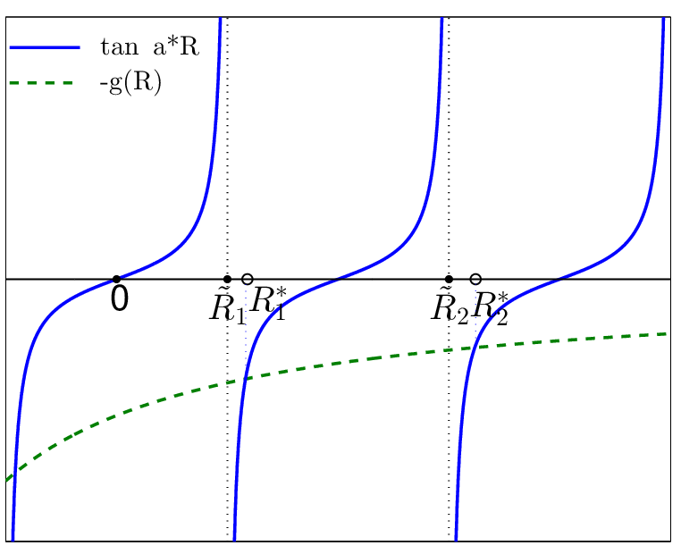

3. If then the density corresponding to the root can not be both positive at the origin and at . Let be the (nontrivial) solution of , then the corresponding density is given by
A direct evaluation of leads to
Using (19a) and the inequality , we get
Therefore, since ,
These estimates imply that , while the physical density must be nonnegative on the support.
4. The density corresponding to the root is decreasing and strictly positive on its support . Let us first show that . Assume that this is not the case, then . Since for , then
This, together with and , implies that , leading to a contradiction. Therefore, combining with the fact that and , both and must be positive.
It is easy to check that is a decreasing function till its first local minimum , determined by
or equivalently with . Using the definition (22a) of ,
Since is the unique root of the strictly increasing function on the interval , the fact that implies that . Therefore, the density is a decreasing function on , as illustrated in Figure 3(b). Finally, evaluating at the boundary , we get
This shows that , and therefore is strictly positive on its support, which completes the proof. ∎
4 Existence theory of flock profiles in two dimension
We now turn our attention to two space dimensions, where the involved Bessel functions do not reduce to standard trigonometric expressions. For ,
| (23) |
and
| (24a) | |||
| (24b) | |||
| (24c) | |||
The numerical investigations carried out in [12] led to the assertion that flock profiles can only be found when . As in the three-dimensional case, we can now give a rigorous theorem and proof thanks to the explicit computations of Section 2.
Theorem 4.1.
Let be a Quasi-Morse potential in space dimension with parameters within the biologically relevant regime . Then flock profiles exist if and only if or equivalently .
We begin by proving a general monotonicity result on the ratio of two modified Bessel functions, which will be used repeatedly throughout the section.
Lemma 4.2.
For any , the functions , and are strictly decreasing functions on .
Proof.
Let , which is positive and smooth on . We take the derivative of both sides of and use the recurrence relation
which is equivalent to the differential equation for
| (25) |
Taking the derivative of (25) w.r.t ,
| (26) |
We can first get the “boundary conditions” for near the origin or infinity, by asymptotic expansions. When is close to the origin, one uses (39) to deduce
for and
for . When is large, by the asymptotic expansion (40), one gets
Therefore, when is near origin and . Moreover, has no local maximum on . Otherwise if there is a local maximum at , then , . On the other hand, by (26), , a contradiction.
Next, we show that on . If at some point , then by the fact that when is large, must have a local maximum on (because first increases and then decreases). If at , then by (26), . Hence there is a point , such that , and it is reduced to the previous case. Therefore, in either situation, there exists a local maximum on , contradicting the statement proved in the last paragraph. This concludes the proof of the strict monotonicity of on .
Similarly, the monotonicity of and can be proved, by using the second-order ODEs
and
In all the three cases, the key ingredients of the proof are the right “boundary condition” near the origin and infinity, and at any point such that . ∎
Lemma 4.2 is needed in the proof of Theorem 4.1, where contrary to the three-dimensional counterpart, the ratios of Bessel functions do not simplify for even dimensions. The structure of the proof given below would apply in a similar fashion in three dimensions to obtain Theorem 3.1 if the simplified expressions (19a)–(19c) were omitted. We begin with a discussion of the case for any dimensions.
Proof.
(Theorem 4.1) Suppose . Then, in general dimension ,
as and the strict monotonicity of is provided by Lemma 4.2. Hence, no real positive roots of exist in any dimension. Let us return to the case and suppose , then by (23) and can be expressed as
| (27) |
using (24c). The coefficient of is obviously negative. By the monotonicity of ,
This implies that . Therefore, there is no flock profile when .
Next, consider the case . The determinant of the coefficient matrix is given as
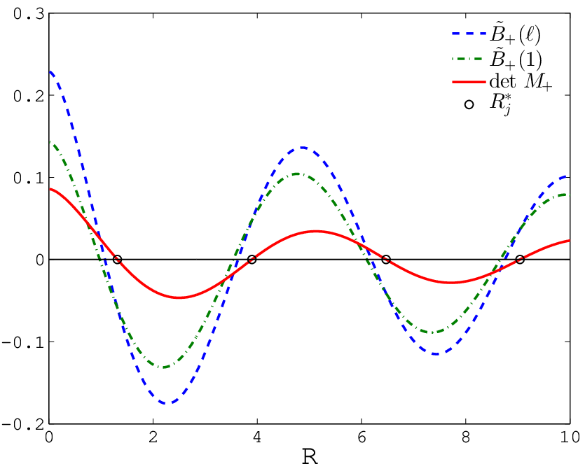
Let be the simple zeros of , then by the relation , are also the critical points of . Since has alternating signs, has at least one root on and therefore, infinitely many roots on .
Let be the first root in the first interval , then we must have as illustrated in Figure 4(a). Otherwise, if , using (24a) we deduce
On the other hand, since is positive together with the monotonicity of ,
and consequently,
| (28) | ||||
| (29) |
contradicting the fact that satisfies .
Since , then and have the same sign. If the corresponding density at the origin is nonnegative, then both and are positive. We first factor out from the equation , i.e.,
Substituting this into , we conclude
Finally, since is smaller than the first local minimum of , is decreasing on . Thus, the strict positivity of on results from the strict positivity of . ∎

Remark.
Theorem 4.1 lacks the uniqueness result of Theorem 3.1. However, numerical investigations point towards a uniqueness result similar to three dimensions. As an example, we illustrate and the densities associated to its roots for a set of parameters investigated in [12] in Figure 4. To prove uniqueness in two dimensions, the possibility of nonnegative densities for roots and the possibility of multiple solutions in have to be ruled out.
5 Further properties of flock profiles for the Quasi-Morse potential
Let us remark that there are parameters such that the convolution equation (6) has a solution even though they do not belong to the biologically relevant cases. Flock profiles, as defined in Definition 1.1, can be found by similar proofs as in the previous two sections in the region , where has a positive global maximum. This family of flock profiles are in fact those that are corresponding stable steady solution in the time-reversed first-order swarming system (33), and are not observed in simulations, since they are unstable, both for first-order and second-order particle models.
The proofs in the previous two sections also indicate the dependence of the flock profiles with respect to the size of their support parameterized by , at least in the asymptotic limit of approaching its lower and upper limit. For example in 3D, since and , we have .
In three dimensions, for fixed parameters and , if is close to its upper limit in the parameter space, then is close to zero, and for the auxiliary function defined in (22a), we have
The desired root can be approximated from the simplified equation , which is simply in the last step of the proof of Theorem 3.1. Therefore, as increases to , the radius of support of the flock profile also approaches the first minimum of .
On the other hand, if is close to its lower limit , diverges, and
Since is close to and the desired root is close to zero, can be further simplified to
a constant proportional to . From the asymptotic equation , approaches from above, or .
Summarizing, in term of the original parameters , and ,
| (30) |
when is close to and
| (31) |
when is close to . The comparison between these asymptotic expansions of with those obtained from solving by a root-finding algorithm is shown in Figure 5. Substituting the above expressions into , the expansions for and can be obtained accordingly.


In two dimensions, the leading-order asymptotic expansion of can be derived similarly. When is close to zero, is large and . Assuming for some , then
and
Since as , we have and unless the leading order in vanishes. Therefore, the coefficient is determined by
where the positive number is smaller than the first positive root of since this equation has infinitely many roots.
When is close to , is small and is
From the fact that diverges,
Therefore, only if vanishes to have both terms above of order . In other words, converges to the first positive root of . Consequently, the expansions of in two dimensions can be obtained.
6 Variants of Morse-type potentials
In the previous sections, we have shown that flock profiles precisely exist for the Quasi-Morse potential when the parameters and are in the region , see Figure 1. The conditions and ensure that the potential is biologically relevant since it has a positive global minimum, while the condition is related to the non-H-stability of the potential. A similar result for the Morse-potential is presented in [15]. The claim, that a positive global minimum of the potential and non-H-stability imply existence of compactly supported flock solutions, also seems to be true for other similar potentials of the form , but concentration of density may appear and the dimensionality of the support can vary with . We show some numerical evidence in support of the claim for the generalised Morse-like potential with
| (32) |
For this potential, the non-H-stability condition is the same but the biologically relevant region is given by and . The numerical simulations were conducted by finding stationary profiles of the first-order swarming system of particles given by
| (33) |
Taking these positions and the common velocity with as initial data for the second-order system (2), the resulting stationary solution is stable [10].
In Figure 6 (a), we observe generic non-concentrated compactly supported flock profiles for the exponent and that appear to converge to a continuous distribution as . The same phenomena are observed for exponents .
However, this type of aggregation cannot be expected for exponents . For , the density seems to concentrate towards its boundary when approaches , as illustrated in Figure 6 (b). For , we observe mixed dimensionality of the support in Figure 6 (c) for varying exponents approaching the limit case . Flock profiles seem to bifurcate as leading to a concentration on a ring plus a continuous distribution inside. To our knowledge this surprising phenomenon of mixed dimensionality of the support has only been reported in 3D simulations in [30, 2] for purely attractive-repulsive potentials. In a swarming model of locusts in 2D using Morse potential [29, 4, 5], the concentration of densities on the (one-dimensional) ground can also be reproduced from obervations in nature, by including additional external gravity force.


This concentration and dimensionality of the support of the steady density is related to the singularity of near the origin, as has already been demonstrated in [2]. Here, we have to argue by numerical experiments as existence proofs will be difficult, partially because of the absence of explicit formulas. Similarly discussions can be found in [22] for solutions perturbed from a ring solution, and in [4, 5] for extensive 1D examples with -concentration on a domain boundary. However, a detailed analytical investigation of these and other properties, such as the integrability of the density near the boundary, remains a challenging question for the potentials considered.
7 Conclusion
In this paper, we analyzed the solvability of convolution equations that describe particular solutions in aggregation or self-propelled interacting particle models equipped with radially symmetric interaction potentials. Although models such as (2) and (33) have been frequently used with various potentials, the analysis of particular solutions such as flock profiles and rotating mills is far from complete. We concentrated our attention on the study of flock profiles, defined as compactly supported continuous radial densities satisfying equation (6). Focusing on the case of Quasi-Morse potentials introduced in [12], we were able to analytically study the parameter phase portrait of these potentials in two and three dimensions, and to prove analytically solvability conditions for flock profiles that were previously asserted numerically. These findings are summarized in Figure 1: The aggregate potential parameter determines solvability in the biologically relevant parameter regimes. In three dimensions, we showed existence and uniqueness of flock profiles for , whereas no flock profiles exists if . The same non-existence result holds true in two dimensions, where flock profiles are shown to exist if and only if . The proof of our main Theorems 3.1 and 4.1 is based on a technical discussion of the Bessel functions contained in the definition of the Quasi-Morse potentials and the explicit formulas of their flock profiles obtained in [12]. First, an explicit expression for the convolution was derived for the three cases and . Then, a detailed analysis of the resulting expressions enabled us to establish our theorems. A central observation is the fact that the question of existence and uniqueness of flock profiles reduces to the study of roots of a determinant of the coefficient matrix . Due to the simpler functions involved, results obtained in three dimensions are slightly stronger than in two dimensions.
In summary, this paper is the first to our knowledge to complete a full analytical study of the existence of flock profiles in the biologically relevant parameter regime, at least for a particular potential. The analysis of the Quasi-Morse potential and our simulations seem to indicate the existence of flock solutions as long as the potential has a unique positive global minimum and is not H-stable. Characterizing when they are flock profiles is challenging and related to the dimensionality of the support of minimizers of the interaction energy [2]. Proving or disproving these claims for other potentials in (2), such as the Morse-type potentials (32), as well as the question of stability of such states in the dynamics of the associated PDEs however remains an open and challenging problem.
Appendix A Bessel functions and Modified Bessel functions
In this paper, Bessel functions and modified Bessel functions are heavily used to study the analytically more tractable Quasi-Morse type potential (7). The definitions and key properties of these Bessel functions, found in standard textbook in special functions [27], are collected below for the readers’ convenience.
The Bessel functions of the first kind and of the second kind are solutions of the equation
| (34) |
that are finite and singular at the origin for positive , respectively. The modified Bessel function of the first kind and of the second kind are solutions of the equation
| (35) |
that are exponentially growing and decaying, respectively.
In two and three dimensions considered in this paper, the (modified) Bessel functions with negative order can be rewritten in terms of those with positive order. In particular, in two dimensions we have
| (36) |
and in three dimensions, we have the following explicit representations using the well-known (hyperbolic) trigonometric functions
| (37a) | |||
| (37b) | |||
| (37c) |
Recursive relations. In the proof of the Lemma 4.2, the following recursive relations for the modified Bessel function and are used
| (38a) | |||
| (38b) | |||
| In the equivalent integral form, the following are used to evaluate (14) and in the proof of Proposition 2.1 in Appendix B, | |||
| (38c) | |||
Asymptotic expansions. In the proof of the Lemma 4.2, the following asymptotic expansions of for are also needed. When is close to the origin,
| (39) |
with the Euler constant . When is large,
| (40) |
Appendix B Proof of Proposition 2.1
Here, we focus on the integrals related to , because those related to are obtained by evaluating at and .
First, we evaluate the integral (14) when are the linearly independent functions in the general solution (9), i.e., the constant , , and respectively. When ,
When , using (38c) and integration by parts, we get
and hence
| (43a) | ||||
| (43b) | ||||
| (43c) | ||||
| (43d) | ||||
Here the terms inside the square bracket of (43b) or (43c) are equal to or , by the recursive relations (38a) and the identity (41).
Finally when , using (42c) and (42d),
Putting all the integrals together, we conclude the explicit form (15) for the convolution . For example, when , , collecting the terms in the integral (13), we get
The first term is the desired constant , and the factor in the second term vanishes by the definition of . The rest of the terms are a linear combination of and , and they can be rearranged into the form (9) with the coefficient of normalized to one to simplify the later proofs. The explicit form for when or has similar structures, and its simplification leads to the final expression (15).
Acknowledgments
JAC was supported by projects MTM2011-27739-C04-02 and 2009-SGR-345 from Agència de Gestió d’Ajuts Universitaris i de Recerca-Generalitat de Catalunya. JAC acknowledges support from the Royal Society through a Wolfson Research Merit Award. JAC, YH, and SM were supported by Engineering and Physical Sciences Research Council grant number EP/K008404/1.
References
- [1] G. Albi, D. Balagué, J. A. Carrillo, and J. VonBrecht. Stability analysis of flock and mill rings for 2nd order models in swarming. to appear in SIAM J. Appl. Math., 2013.
- [2] D. Balagué, J. A. Carrillo, T. Laurent, and G. Raoul. Dimensionality of local minimizers of the interaction energy. Arch. Rat. Mech. Anal., 209(3):1055–1088, 2013.
- [3] D. Balagué, J. A. Carrillo, T. Laurent, and G. Raoul. Nonlocal interactions by repulsive-attractive potentials: radial ins/stability. Phys. D, 260:5–25, 2013.
- [4] A. J. Bernoff and C. M. Topaz. A primer of swarm equilibria. SIAM J. Appl. Dyn. Syst., 10(1):212–250, 2011.
- [5] Andrew J. Bernoff and Chad M. Topaz. Nonlocal Aggregation Models: A Primer of Swarm Equilibria. SIAM Rev., 55(4):709–747, 2013.
- [6] A. L. Bertozzi, J. A. Carrillo, and T. Laurent. Blow-up in multidimensional aggregation equations with mildly singular interaction kernels. Nonlinearity, 22(3):683–710, 2009.
- [7] A. L. Bertozzi, J. H. von Brecht, H. Sun, T. Kolokolnikov, and D. Uminsky. Ring patterns and their bifurcations in a nonlocal model of biological swarms. to appear in Comm. Math. Sci., 2013.
- [8] S. Camazine, J.-L. Deneubourg, N. R. Franks, J. Sneyd, G. Theraulaz, and E. Bonabeau. Self-organization in biological systems. Princeton Studies in Complexity. Princeton University Press, Princeton, NJ, 2003. Reprint of the 2001 original.
- [9] J. A. Carrillo, M. R. D’Orsogna, and V. Panferov. Double milling in self-propelled swarms from kinetic theory. Kinet. Relat. Models, 2(2):363–378, 2009.
- [10] J. A. Carrillo, Y. Huang, and S. Martin. Nonlinear stability of flock solutions in second-order swarming models. Nonlinear Anal. Real World Appl., 17:332–343, 2014.
- [11] J. A. Carrillo, A. Klar, S. Martin, and S. Tiwari. Self-propelled interacting particle systems with roosting force. Math. Mod. Meth. Appl. Sci, 20:1533–1552, 2010.
- [12] J. A. Carrillo, S. Martin, and V. Panferov. A new interaction potential for swarming models. Phys. D, 260:112–126, 2013.
- [13] Y.-L. Chuang, M. R. D’Orsogna, D. Marthaler, A. L. Bertozzi, and L. S. Chayes. State transitions and the continuum limit for a 2D interacting, self-propelled particle system. Phys. D, 232(1):33–47, 2007.
- [14] I. D. Couzin and J. Krause. Self-organization and collective behavior of vertebrates. Adv. Study Behav., 32:1–67, 2003.
- [15] M. R. D’Orsogna, Y.-L. Chuang, A. L. Bertozzi, and L. S Chayes. Self-propelled particles with soft-core interactions: patterns, stability, and collapse. Phys. Rev. Lett., 96(10):104302, 2006.
- [16] R. C. Fetecau and Y. Huang. Equilibria of biological aggregations with nonlocal repulsive–attractive interactions. Phys. D, 260:49–64, 2013.
- [17] R. C. Fetecau, Y. Huang, and T. Kolokolnikov. Swarm dynamics and equilibria for a nonlocal aggregation model. Nonlinearity, 24(10):2681–2716, 2011.
- [18] H. Hildenbrandt, C. Carere, and C. K. Hemelrijk. Self-organised complex aerial displays of thousands of starlings: a model. Behavioral Ecology, 107(21):1349–1359, 2010.
- [19] D. D. Holm and V. Putkaradze. Aggregation of finite-size particles with variable mobility. Phys. Rev. Lett., 95:226106, 2005.
- [20] D. D. Holm and V. Putkaradze. Formation of clumps and patches in selfaggregation of finite-size particles. Phys. D, 220(2):183–196, 2006.
- [21] A. Huth and C. Wissel. The simulation of the movement of fish schools. J. Theor. Biol., 156:365–385, 1992.
- [22] T. Kolokolnikov, Y. Huang, and M. Pavlovski. Singular patterns for an aggregation model with a confining potential. Phys. D, 260:65–76, 2013.
- [23] T. Kolokonikov, H. Sun, D. Uminsky, and A. Bertozzi. Stability of ring patterns arising from 2d particle interactions. Phys. Rev. E, 84(1):015203, 2011.
- [24] H. Levine, W.-J. Rappel, and I. Cohen. Self-organization in systems of self-propelled particles. Phys. Rev. E, 63:017101, Dec 2000.
- [25] E. H. Lieb and M. Loss. Analysis, volume 14 of Graduate Studies in Mathematics. American Mathematical Society, Providence, RI, second edition, 2001.
- [26] R. Lukeman, Y.X. Li, and L. Edelstein-Keshet. Inferring individual rules from collective behavior. Proc. Natl. Acad. Sci. U.S.A., 107(28):12576–12580, 2010.
- [27] W. Magnus, F. Oberhettinger, and R. P. Soni. Formulas and theorems for the special functions of mathematical physics. Springer-Verlag, New York, 1966.
- [28] A. Mogilner and L. Edelstein-Keshet. A non-local model for a swarm. J. Math. Biol., 38:534–570, 1999.
- [29] C. M. Topaz, A. J. Bernoff, S. Logan, and W. Toolson. A model for rolling swarms of locusts. Eur. Phys. J. Spec. Top., 157(1):93–109, 2008.
- [30] J. H. von Brecht and D. Uminsky. On soccer balls and linearized inverse statistical mechanics. J. Nonlinear Sci., 22(6):935–959, 2012.
- [31] J. H. von Brecht, D. Uminsky, T. Kolokolnikov, and A. L. Bertozzi. Predicting pattern formation in particle interactions. Math. Models Methods Appl. Sci., 22:1140002, 31, 2012.