When are Overcomplete Topic Models Identifiable?
Uniqueness of Tensor Tucker Decompositions
with Structured Sparsity
Abstract
Overcomplete latent representations have been very popular for unsupervised feature learning in recent years. In this paper, we specify which overcomplete models can be identified given observable moments of a certain order. We consider probabilistic admixture or topic models in the overcomplete regime, where the number of latent topics can greatly exceed the size of the observed word vocabulary. While general overcomplete topic models are not identifiable, we establish generic identifiability under a constraint, referred to as topic persistence. Our sufficient conditions for identifiability involve a novel set of “higher order” expansion conditions on the topic-word matrix or the population structure of the model. This set of higher-order expansion conditions allow for overcomplete models, and require the existence of a perfect matching from latent topics to higher order observed words. We establish that random structured topic models are identifiable w.h.p. in the overcomplete regime. Our identifiability results allows for general (non-degenerate) distributions for modeling the topic proportions, and thus, we can handle arbitrarily correlated topics in our framework. Our identifiability results imply uniqueness of a class of tensor decompositions with structured sparsity which is contained in the class of Tucker decompositions, but is more general than the Candecomp/Parafac (CP) decomposition.
Keywords: Overcomplete representations, topic models, generic identifiability, tensor decomposition.
1 Introduction
The performance of many machine learning methods is hugely dependent on the choice of data representations or features. Overcomplete representations, where the number of features can be greater than the dimensionality of the input data, have been extensively employed, and are arguably critical in a number of applications such as speech and computer vision [1]. Overcomplete representations are known to be more robust to noise, and can provide greater flexibility in modeling [2]. Unsupervised estimation of overcomplete representations has been hugely popular due to the availability of large-scale unlabeled samples in many applications.
A probabilistic framework for incorporating features posits latent or hidden variables that can provide a good explanation to the observed data. Overcomplete probabilistic models can incorporate a much larger number of latent variables compared to the observed dimensionality. In this paper, we characterize the conditions under which overcomplete latent variable models can be identified from their observed moments.
For any parametric statistical model, identifiability is a fundamental question of whether the model parameters can be uniquely recovered given the observed statistics. Identifiability is crucial in a number of applications where the latent variables are the quantities of interest, e.g. inferring diseases (latent variables) through symptoms (observations), inferring communities (latent variables) via the interactions among the actors in a social network (observations), and so on. Moreover, identifiability can be relevant even in predictive settings, where feature learning is employed for some higher level task such as classification. For instance, non-identifiability can lead to the presence of non-isolated local optima for optimization-based learning methods, and this can affect their convergence properties, e.g. see [3].
In this paper, we characterize identifiability for a popular class of latent variable models, known as the admixture or topic models [4, 5]. These are hierarchical mixture models, which incorporate the presence of multiple latent states (i.e. topics) in each document consisting of a tuple of observed variables (i.e. words). Previous works have established that the model parameters can be estimated efficiently using low order observed moments (second and third order) under some non-degeneracy assumptions, e.g. [6, 7, 8]. However, these non-degeneracy conditions imply that the model is undercomplete, i.e., the latent dimensionality (number of topics) cannot exceed the observed dimensionality (word vocabulary size). In this paper, we remove this restriction and consider overcomplete topic models, where the number of topics can far exceed the word vocabulary size.
It is perhaps not surprising that general topic models are not identifiable in the overcomplete regime. To this end, we introduce an additional constraint on the model, referred to as topic persistence. Intuitively, this captures the “locality” effect among the observed words, and is not present in the usual “bag-of-words” or exchangeable topic model. Such local dependencies among observations abound in applications such as text, images and speech, and can lead to a more faithful representation. In addition, we establish that the presence of topic persistence is central towards obtaining model identifiability in the overcomplete regime, and we provide an in-depth analysis of this phenomenon in this paper.
1.1 Summary of results
In this paper, we provide conditions for generic 11 1 A model is generically identifiable, if all the parameters in the parameter space are identifiable, almost surely. Refer to Definition 1 for more discussion. model identifiability of overcomplete topic models given observable moments of a certain order (i.e., having a certain number of words in each document). We introduce the notion of topic persistence, and analyze its effect on identifiability. We establish identifiability in the presence of a novel combinatorial object, referred to as perfect -gram matching, in the bipartite graph from topics to words. Finally, we prove that random structured topic models satisfy these criteria, and are thus identifiable in the overcomplete regime.
Persistent Topic Model:
We first introduce the -persistent topic model, where the parameter determines the persistence level of a common topic in a sequence of successive words. For instance, in Figure 1, the sequence of successive words share a common topic , and similarly, the words share topic , and so on. The -persistent model reduces to the popular “bag-of-words” model, when , and to the single topic model (i.e. only one topic in each document) when . Intuitively, topic persistence aids identifiability since we have multiple views of the common hidden topic generating a sequence of successive words. We establish that the bag-of-words model (with ) is too non-informative about the topics in the overcomplete regime, and is therefore, not identifiable. On the other hand, -persistent overcomplete topic models with can become identifiable, and we establish a set of transparent conditions for identifiability.

Deterministic Conditions for Identifiability:
Our sufficient conditions for identifiability are in the form of expansion conditions from the latent topic space to the observed word space. In the overcomplete regime, there are more topics than words in the vocabulary, and thus it is impossible to have expansion on the bipartite graph from topics to words, i.e., the graph encoding the sparsity pattern of the topic-word matrix. Instead, we impose an expansion constraint from topics to “higher order” words, which allows us to incorporate overcomplete models. We establish that this condition translates to the presence of a novel combinatorial object, referred to as the perfect n-gram matching, on the topic-word bipartite graph. Intuitively, the perfect -gram matching condition implies “diversity” among the higher-order word supports for different topics which leads to identifiability. In addition, we present trade-offs among the following quantities: number of topics, size of the word vocabulary, the topic persistence level, the order of the observed moments at hand, the minimum and maximum degrees of any topic in the topic-word bipartite graph, and the Kruskal rank [9] of the topic-word matrix, under which identifiability holds. To the best of our knowledge, this is the first work to provide conditions for characterizing identifiability of overcomplete topic models with structured sparsity.
Identifiability of Random Structured Topic Models:
We explicitly characterize the regime of identifiability for the random setting, where each topic is randomly supported on a set of words, i.e. the bipartite graph is a random graph. For this random model with topics, -dimensional word vocabulary, and topic persistence level , when and , for all topics , the topic-word matrix is identifiable from order observed moments with high probability. Intuitively, the upper bound on the degrees is needed to limit the overlap of word supports among different topics in the overcomplete regime: as the number of topics increases (i.e., increases in the above degree bound), the degree needs to be correspondingly smaller to ensure identifiability, and we make this dependence explicit. Intuitively, as the extent of overcompleteness increases, we need sparser connections from topics to words to ensure sufficient diversity in the word supports among different topics. The lower bound on the degrees is required so that there are enough edges in the topic-word bipartite graph so that various topics can be distinguished from one another. Furthermore, we establish that the size condition for identifiability is tight.
Implications on Uniqueness of Overcomplete Tucker and CP Tensor Decompositions:
We establish that identifiability of an overcomplete topic model is equivalent to uniqueness of decomposition of the observed moment tensor (of a certain order). Our identifiability results for persistent topic models imply uniqueness of a structured class of tensor decompositions, which is contained in the class of Tucker decompositions, but is more general than the candecomp/parafac (CP) decomposition [10]. This sub-class of Tucker decompositions involves structured sparsity and symmetry constraints on the core tensor, and sparsity constraints on the inverse factors of the Tucker decomposition. The structural constraints on the Tucker tensor decomposition are related to the topic model as follows: the sparsity and symmetry constraints on the core tensor are related to the persistence property of the topic model, and the sparsity constraints on the inverse factors are equivalent to the sparsity constraints on the topic-word matrix. For -persistent topic model with (bag-of-words model), the tensor decomposition is a general Tucker decomposition, where the core tensor is fully dense, while for (single-topic model), the tensor decomposition reduces to a CP decomposition, i.e. the core tensor is a diagonal tensor. For a finite persistence level , in between these two extremes, the core tensor satisfies certain sparsity and symmetry constraints, which becomes crucial towards establishing identifiability in the overcomplete regime.
1.2 Overview of Techniques
We now provide a short overview of the techniques employed in this paper.
Recap of Identifiability Conditions in Under-complete Setting (Expansion Conditions on Topic-Word Matrix):
Our approach is based on the recent results of [7], where conditions for identifiability of topic models are derived, given pairwise observed moments (specifically, co-occurrence of word-pairs in documents). Consider a topic model with topics and observed word vocabulary of size . Let denote the topic-word matrix. Expansion conditions are imposed in [7] on the topic-word bipartite graph which imply that (generically) the sparsest vectors in the column span of , denoted by Col, are the columns of themselves. Thus the topic-word matrix is identifiable from pairwise moments under expansion constraints. However, these expansion conditions constrain the model to be under-complete, i.e., the number of topics , the size of the word vocabulary. Therefore, the techniques derived in [7] are not directly applicable here since we consider overcomplete models.
Identifiability in Overcomplete Setting and Why Topic-Persistence Helps:
Pairwise moments are thus not sufficient for identifiability of overcomplete models, and the question is whether higher order moments can yield identifiability. We can view the higher order moments as pairwise moments of another equivalent topic model, which enables us to apply the techniques of [7]. The key question is whether we have expansion in the equivalent topic model, which implies identifiability. For a general topic model (without any topic persistence constraints), it can be shown that for identifiability, we require expansion of the -order Kronecker product of the original topic-word matrix , denoted by , when given access to -order moments, for any integer . In the overcomplete regime where , cannot expand, and therefore, overcomplete models are not identifiable in general. On the other hand, we show that imposing the constraint of topic persistence can lead to identifiability. For a -persistent topic model, given -order moments, we establish that identifiability occurs when the -order Khatri-Rao product of , denoted by , expands. Note that the Khatri-Rao product is a sub-matrix of the Kronecker product , and the Khatri-Rao product can expand as long as . Thus, the property of topic persistence is central towards achieving identifiability in the overcomplete regime.
First-Order Approach for Identifiability of Overcomplete Models (Expansion of -gram Topic-Word Matrix):
We refer to as the -gram topic-word matrix, and intuitively, it relates topics to -tuple words. Imposing the expansion conditions derived in [7] on implies that (generically) the sparsest vectors in Col, are the columns of themselves. Thus, the topic-word matrix is identifiable from -order moments for a -persistent topic model. We refer to this as the “first-order” approach since we directly impose the expansion conditions of [7] on , without exploiting the additional structure present in .
Why the First-Order Approach is not Enough:
Note that matrix relates topics to -tuples of words. Thus, the entries of are highly correlated, even if the original topic-word matrix is assumed to be randomly generated. It is non-trivial to derive conditions on , so that expands. Moreover, we establish that fails to expand on “small” sets, as required in [7], when the degrees are sufficiently different 22 2 For to expand on a set of size , it is necessary that , where and are the minimum and maximum degrees, and is the extent of overcompleteness: . When the model is highly overcomplete (large ) and we require small set expansion (small ), the degrees need to be nearly the same. Thus, it is desirable to impose expansion only on large sets, since it allows for more degree diversity.. Thus, the first-order approach is highly restrictive in the overcomplete setting.
Incorporating Rank Criterion:
Note that is highly structured: the columns of matrix possess a tensor 33 3 When any column of (of length ) is reshaped as a -order tensor , the tensor is rank . rank of , when . This can be incorporated in our identifiability criteria as follows: we provide conditions under which the sparsest vectors in Col, which also possess a tensor rank of , are the columns of themselves. This implies identifiability of a -persistent topic model, when given access to -order moments. Note that when a small number of columns of are combined, the resulting vector cannot possess a tensor rank of , and thus, we can rule out that such sparse combinations of columns using the rank criterion. The maximum such number is at least the Kruskal rank 44 4 The Kruskal rank is the maximum number such that every -subset of columns of are linearly independent. Note that the Kruskal rank is equal to the rank of , when has full column rank. But this cannot happen in the overcomplete setting. of . Thus, sparse combinations of columns of (up to the Kruskal rank) can be ruled out using the rank criterion, and we require expansion on only on large sets of topics (of size larger than the Kruskal rank). This agrees with the intuition that when the topic-word matrix has a larger Kruskal rank, it should be easier to identify , since the Kruskal rank is related to the mutual incoherence 55 5 It is easy to show that , where are any pair of columns of . Thus, higher incoherence leads to a larger kruskal rank. among the columns of , see [11].
Notion of Perfect -gram Matching and Final Identifiability Conditions:
Thus, we establish identifiability of overcomplete topic models subject to expansion conditions on sets of size larger than the Kruskal rank of the topic-word matrix . However, it is desirable to impose transparent and interpretable conditions directly on for identifiability. We introduce the notion of perfect -gram matching on the topic-word bipartite graph, which ensures that each topic can be uniquely matched to a -tuple word. This combined with a lower bound on the Kruskal rank provides the final set of deterministic conditions for identifiability of the overcomplete topic model. Intuitively, we require that the columns of be sparse, while still maintaining a large enough Kruskal rank; in other words, the topics have to be sparse and have sufficiently diverse word supports. Thus, we establish identifiability under a set of transparent conditions on the topic-word matrix , consisting of perfect -gram matching condition and a lower bound on the Kruskal rank of .
Analysis under Random-Structured Topic-Word Matrices:
Finally, we establish that the derived deterministic conditions are satisfied when the topic-word bipartite graph is randomly generated, as long as the degrees satisfy certain lower and upper bounds. Intuitively, a lower bound on the degrees of the topics is required to have degree concentration on various subsets so that expansion can occur, while the upper bound is required so that the Kruskal rank of the topic-word matrix is large enough compared to the sparsity level. Here, the main technical result is establishing the presence of a perfect -gram matching in a random bipartite graph with a wide range of degrees. We present a greedy and a recursive mechanism for constructing such a -gram matching for overcomplete models, which can be relevant even in other settings. For instance, our results imply the presence of a perfect matching when the edges of a bipartite graph are correlated in a structured manner, as given by the Khatri-Rao product.
1.3 Related works
We now summarize some recent related works in the area of identifiability and learning of latent variable models.
Identifiability, learning and applications of overcomplete latent representations:
Many recent works employ unsupervised estimation of overcomplete features for higher level tasks such classification, e.g. [12, 13, 14, 1], and record huge gains over other approaches in a number of applications such as speech recognition and computer vision. However, theoretical understanding regarding learnability or identifiability of overcomplete representations is far more limited.
Overcomplete latent representations have been analyzed in the context of the independent components analysis (ICA), where the sources are assumed to be independent, and the mixing matrix is unknown. In the overcomplete or under-determined regime of the ICA, there are more sources than sensors. Identifiability and learning of the overcomplete ICA reduces to the problem of finding an overcomplete candecomp/parafac (CP) tensor decomposition. The classical result by Kruskal provides conditions for uniqueness of a CP decomposition [9, 15], with recent extensions to the notion of robust identifiability [16]. These results provide conditions for strict identifiability of the model, and here, the dimensionality of the latent space is required to be of the same order as the observed space dimensionality. In contrast, a number of recent works analyze generic identifiability of overcomplete CP decomposition, which is weaker than strict identifiability, e.g. [17, 18, 19, 20, 21, 22, 23]. These works assume that the factors (i.e. the components) of the CP decomposition are generically drawn and provide conditions for uniqueness. They allow for the latent dimensionality to be much larger (polynomially larger) than the observed dimensionality. These results on the uniqueness of CP decompositions also lead to identifiability of other latent variable models, such as latent tree models, e.g. [24, 25], and the single-topic model, or more generally latent Dirichlet allocation (LDA). Recently Goyal et. al. [26] proposed an alternative framework for overcomplete ICA models based on the eigen-decomposition of the reweighted covariance matrix (or higher order moments), where the weights are the Fourier coefficients. However, their approach requires independence of sources (i.e. latent topics in our context), which is not imposed here.
In contrast to the above works dealing with the CP tensor decomposition, we require uniqueness for a more general class of tensor decompositions, in order to establish identifiability of topic models with arbitrarily correlated topics. We establish that our class of tensor decomposition is contained in the class of Tucker decompositions which is more general than CP decomposition. Moreover, we explicitly characterize the effect of the sparsity pattern of the factors (i.e., the topic-word matrix) on model identifiability, while all the previous works based on generic identifiability assume fully dense factors (since sparse factors are not generic). For a general overview of tensor decompositions, see [10, 27].
Identifiability and learning of undercomplete/over-determined latent representations:
Much of the theoretical results on identifiability and learning of the latent variable models are limited to non-singular models, which implies that the latent space dimensionality is at most the observed dimensionality. We outline some of the recent works below.
The works of Anandkumar et. al. [28, 29, 6] provide an efficient moment-based approach for learning topic models, under constraints on the distribution of the topic proportions, e.g. the single topic model, and more generally latent Dirichlet allocation (LDA). In addition, the approach can handle a variety of latent variable models such as Gaussian mixtures, hidden Markov models (HMM) and community models [30]. The high-level idea is to reduce the problem of learning of the latent variable model to finding a CP decomposition of the (suitably adjusted) observed moment tensor. Various approaches can then be employed to find the CP decomposition. In [6], a tensor power method approach is analyzed and is shown to be an efficient guaranteed recovery method in the non-degenerate (i.e. undercomplete) setting. Previously, simultaneous diagonalization techniques have been employed for solving the CP decomposition, e.g. [28, 31, 32]. However, these techniques fail when the model is overcomplete, as considered here. We note that some recent techniques, e.g. [20], can be employed instead, albeit at a cost of higher computational complexity for overcomplete CP tensor decomposition. However, it is not clear how the sparsity constraints affect the guarantees of such methods. Moreover, these approaches cannot handle general topic models, where the distribution of the topic proportions is not limited to these classes (i.e. either single topic or Dirichlet distribution), and we require tensor decompositions which are more general than the CP decomposition.
There are many other works which consider learning mixture models when multiple views are available. See [28] for a detailed description of these works. Recently, Rabani et. al. [33] consider learning discrete mixtures given a large number of “views”, and they refer to the number of views as the sampling aperture. They establish improved recovery results (in terms of bounds) when sufficient number of views are available ( views for a -component mixture). However, their results are limited to discrete mixtures or single-topic models, while our setting can handle more general topic models. Moreover, our approach is different since we incorporate sparsity constraints in the topic-word distribution. Another series of recent works by Arora et. al. [34, 8] employ approaches based on non-negative matrix factorization (NMF) to recover the topic-word matrix. These works allow models with arbitrarily correlated topics, as considered here. They establish guaranteed learning when every topic has an anchor word, i.e. the word is uniquely generated from that topic, and does not occur under any other topic. Note that the anchor-word assumption cannot be satisfied in the overcomplete setting.
Our work is closely related to the work of Anandkumar et. al. [7] which considers identifiability and learning of topic models under expansion conditions on the topic-word matrix. The work of Spielman et. al [35] considers the problem of dictionary learning, which is closely related to the setting of [7], but in addition assumes that the coefficient matrix is random. However, these works [7, 35] can handle only the under-complete setting, where the number of topics is less than the dimensionality of the word vocabulary (or the number of dictionary atoms is less than the number of observations in [35]). We extend these results to the overcomplete setting by proposing novel higher order expansion conditions on the topic-word matrix, and also incorporate additional rank constraints present in higher order moments.
Dictionary learning/sparse coding:
Overcomplete representations have been very popular in the context of dictionary learning or sparse coding. Here, the task is to jointly learn a dictionary as well as a sparse selection of the dictionary atoms to fit the observed data. There have been Bayesian as well as frequentist approaches for dictionary learning [2, 36, 37]. However, the heuristics employed in these works [2, 36, 37] have no performance guarantees. The work of Spielman et. al [35] considers learning (undercomplete) dictionaries and provide guaranteed learning under the assumption that the coefficient matrix is random (distributed as Bernoulli-Gaussian variables). Recent works [38, 39] provide generalization bounds for predictive sparse coding, where the goal of the learned representation is to obtain good performance on some predictive task. This differs from our framework since we do not consider predictive tasks here, but the task of recovering the underlying latent representation. Hillar and Sommer [40] consider the problem of identifiability of sparse coding and establish that when the dictionary succeeds in reconstructing a certain set of sparse vectors, then there exists a unique sparse coding, up to permutation and scaling. However, our setting here is different, since we do not assume that a sparse set of topics occur in each document.
2 Model
Notation:
The set is denoted by . Given a set , set denotes all ordered -tuples generated from . The cardinality of a set is denoted by . For any vector (or matrix ), the support is denoted by , and the norm is denoted by , which corresponds to the number of non-zero entries of , i.e., . For a vector , is the diagonal matrix with vector on its diagonal. The column space of a matrix is denoted by . Vector is the -th basis vector, with the -th entry equal to 1 and all the others equal to zero. For and , the Kronecker product is defined as [41]
and for and , the Khatri-Rao product is defined as
2.1 Persistent topic model
In this section, the -persistent topic model is introduced and this imposes an additional constraint, known as topic persistence on the popular admixture model[4, 5, 42]. The -persistent topic model reduces to the bag-of-words admixture model when .
An admixture model specifies a -dimensional vector of topic proportions which generates the observed variables through vectors . This collection of vectors , is referred to as the population structure or the topic-word matrix [42]. For instance, is the conditional distribution of words given topic . The latent variable is a dimensional random vector known as proportion vector. A prior distribution over the probability simplex characterizes the prior joint distribution over the latent variables . In the topic modeling, this is the prior distribution over the topics.
The -persistent topic model has a three-level multi-view hierarchy in Figure 1. number of words (views) are shown in the model for some integer . In this model, a common hidden topic is persistent for a sequence of words . Note that the random observed variables (words) are exchangeable within groups of size , where is the persistence level, but are not globally exchangeable.
We now describe a linear representation of the -persistent topic model, on lines of [6], but with extensions to incorporate persistence. Each random variable is a discrete valued random variable taking one of the possibilities , i.e., for . In the -persistent model, a single common topic is chosen for a sequence of words , i.e., the topic is persistent for successive views. For notational purposes, we equivalently assume that variables , are encoded by the basis vectors . Thus, the variable , is
Given proportion vector , topics , are independently drawn according to the conditional expectation
or equivalently .
Finally, at the bottom layer, each observed variable for , is a discrete-valued -dimensional random variable, where is the size of word vocabulary. Again, we assume that variables , are encoded by the basis vectors , such as
Given the corresponding topic , words , are independently drawn according to the conditional expectation
| (1) |
where vectors , are the conditional probability distribution vectors. The matrix collecting these vectors is the population structure or topic-word matrix.
The -th order moment of observed variables , for some integer , is defined as (in the matrix form) 66 6 Vector is the vector generated by concatenating all vectors .
| (2) |
For the -persistent topic model with number of observations (words) , the corresponding moment is denoted by . Note that to estimate the moment, we require a minimum of words in each document. We can select the first words in each document, and average over the different documents to obtain a consistent estimate of the moment. In this paper, we consider the problem of identifiability when exact moments are available.
The moment characterization of the -persistent topic model is provided in Lemma 1 in Section 4.1. Given , what are the sufficient conditions under which the population structure is identifiable? This is answered in Section 3.
Remark 1.
Note that our results are valid for the more general linear model (more precisely, ), i.e., each column of matrix does not need to be a valid probability distribution. Furthermore, the observed random variables , can be continuous while the hidden ones are assumed to be discrete.
3 Sufficient Conditions for Generic Identifiability
In this section, the identifiability result for the -persistent topic model with access to -th order observed moment is provided. First, sufficient deterministic conditions on the population structure are provided for identifiability in Theorem 1. Next, the deterministic analysis is specialized to a random structured model in Theorem 2.
We now make the notion of identifiability precise. As defined in literature, (strict) identifiability means that the population structure can be uniquely recovered up to permutation and scaling for all . Instead, we consider a more relaxed notion of identifiability, known as generic identifiability.
Definition 1 (Generic identifiability).
We refer to a matrix as generic, with a fixed sparsity pattern when the nonzero entries of are drawn from a distribution which is absolutely continuous with respect to Lebesgue measure 77 7 As an equivalent definition, if the non-zero entries of an arbitrary sparse matrix are independently perturbed with noise drawn from a continuous distribution to generate , then is called generic.. For a given sparsity pattern, the class of population structure matrices is said to be generically identifiable [25], if all the non-identifiable matrices form a set of Lebesgue measure zero.
The -th order moment of hidden variables , denoted by , is defined as
| (3) |
We now provide a set of sufficient conditions for generic identifiability of structured topic models given -th order observed moment. We first start with a natural assumption on the hidden variables.
Condition 1 (Non-degeneracy).
The -th order moment of hidden variables , defined in equation (3), is full rank (non-degeneracy of hidden nodes).
Note that there is no hope of distinguishing distinct hidden nodes without this non-degeneracy assumption. We do not impose any other assumption on hidden variables and can incorporate arbitrarily correlated topics.
Furthermore, we can only hope to identify the population structure up to scaling and permutation. Therefore, we can identify up to a canonical form defined as:
Definition 2 (Canonical form).
Population structure is said to be in canonical form if all of its columns have unit norm.
3.1 Deterministic conditions for generic identifiability
In this section, we consider a fixed sparsity pattern on the population structure and establish generic identifiability when non-zero entries of are drawn from some continuous distribution. Before providing the main result, a generalized notion of (perfect) matching for bipartite graphs is defined. We subsequently impose these conditions on the bipartite graph from topics to words which encodes the sparsity pattern of population structure .
Generalized matching for bipartite graphs
A bipartite graph with two disjoint vertex sets and and an edge set between them is denoted by . Given the bi-adjacency matrix , the notation is also used to denote a bipartite graph. Here, the rows and columns of matrix are respectively indexed by and vertex sets. For any subset , the set of neighbors of vertices in with respect to is defined as , or equivalently, with respect to edge set .
Here, we define a generalized notion of matching for a bipartite graph and refer to it as -gram matching.
Definition 3 ((Perfect) -gram matching).
A -gram matching for a bipartite graph is a subset of edges which satisfies the following conditions.
First, for any , we have . Second, for any , we have .
A perfect -gram matching or -saturating -gram matching for the bipartite graph is a -gram matching in which each vertex in is the end-point of exactly edges in .
In words, in a -gram matching , each vertex is at most the end-point of edges in and for any pair of vertices in (), there exists at least one non-common neighbor in set for each of them ( and ).
As an example, a bipartite graph with and is shown in Figure 2 for which the edge set itself is a perfect 2-gram matching.

Remark 2 (Relationship to other matchings).
The relationship of -gram matching to other types of matchings is discussed below.
- •
Regular matching: For special case , the (perfect) -gram matching reduces to the usual (perfect) matching for bipartite graphs.
- •
-matching: A -matching for a bipartite graph (with equal vertex sizes ) is a subset of edges , where each vertex is connected to edges. Comparing with the proposed perfect -gram matching, -matching does not enforce that the set of neighbors be different, and furthermore, it requires that , which is not possible under the overcomplete setting.
Remark 3 (Necessary size bound).
Consider a bipartite graph with and which has a perfect -gram matching. Note that there are -combinations on side and each combination can at most have one neighbor (a node in which is connected to all nodes in the combination) through the matching, and therefore we necessarily have .
Finally, note that the existence of perfect -gram matching results the existence of perfect -gram matching 88 8 Note that the degree of each node (on matching side ) in the original bipartite graph should be at least ., but the reverse is not true. For example, the bipartite graph with and in Figure 2, has a perfect 2-gram matching, but not a perfect (1-gram) matching (since ).
Identifiability conditions based on existence of perfect -gram matching in topic-word graph
Now, we are ready to propose the identifiability conditions and result.
Condition 2 (Perfect -gram matching on ).
The bipartite graph between hidden and observed variables, has a perfect -gram matching.
The above condition implies that the sparsity pattern of matrix is appropriately scattered in the mapping from hidden to observed variables to be identifiable. Intuitively, it means that every hidden node can be distinguished from another hidden node by its unique set of neighbors under the corresponding -gram matching.
Furthermore, condition 2 is the key to be able to propose identifiability in the overcomplete regime. As stated in the size bound in Remark 3, for , the number of hidden variables can be more than the number of observed variables and we can still have perfect -gram matching.
Definition 4 (Kruskal rank, [15]).
The Kruskal rank or the krank of matrix is defined as the maximum number such that every subset of columns of is linearly independent.
Note that krank is different from the general notion of matrix rank and it is a lower bound for the matrix rank, i.e., .
Condition 3 (Krank condition on ).
The Kruskal rank of matrix satisfies the bound , where is the maximum node degree of any column of .
In the overcomplete regime, it is not possible for to be full column rank and . However, note that a large enough krank ensures that appropriate sized subsets of columns of are linearly independent. For instance, when , any two columns cannot be collinear and the above condition rules out the collinear case for identifiability. In the above condition, we see that a larger krank can incorporate denser connections between topics and words.
The main identifiability result under a fixed graph structure is stated in the following theorem for , where is the topic persistence level. The identifiability result relies on having access to the -th order moment of observed variables , defined in equation (2) as
for some integer .
Theorem 1 (Generic identifiability under deterministic topic-word graph structure).
Let in equation (2) be the -th order observed moment of the -persistent topic model for some integer . If the model satisfies conditions 1, 2 and 3, then, for any , all the columns of population structure are generically identifiable from . Furthermore, the -th order moment of the hidden variables, denoted by , is also generically identifiable.
The theorem is proved in Appendix A.
It is seen that the population structure is identifiable, given any observed moment of order at least . Increasing the order of observed moment results in identifying higher order moments of the hidden variables.
The above theorem does not cover the case when the persistence level . This is the usual bag-of-words admixture model. Identifiability of this model has been studied earlier [7] and we recall it below.
Remark 4 (Bag-of-words admixture model, [7]).
Given -th order observed moments with , the structure of the popular bag-of-words admixture model and the -th order moment of hidden variables are identifiable, when is full column rank and the following expansion condition holds [7]
| (4) |
Our result for in Theorem 1, provides identifiability in the overcomplete regime with weaker matching condition 2 and krank condition 3. The matching condition 2 is weaker than the above expansion condition which is based on the perfect matching and hence, does not allow overcomplete models. Furthermore, the above result for the bag-of-words admixture model requires full column rank of which is more stringent than our krank condition 3.
Remark 5 (Kruskal rank and degree diversity).
Condition 3 requires that the Kruskal rank of the topic-word matrix be large enough compared to the maximum degree of the topics. Intuitively, a larger Kruskal rank ensures enough diversity in the word supports among different topics under a higher level of sparsity. This Kruskal rank condition also allows for more degree diversity among the topics, when the topic persistence level . On the other hand, for the bag-of-words model (), using (4) implies that , where are the minimum and maximum degrees of the topics. Thus, we provide identifiability results with more degree diversity when higher order moments are employed.
Remark 6 (Recovery using optimization).
It turns out that our conditions for identifiability imply that the columns of the -gram matrix , defined in Definition 6, are the sparsest vectors in , having a tensor rank of one. See Appendix A. This implies recovery of the columns of through exhaustive search, which is not efficient. Efficient -based recovery algorithms have been analyzed in [43, 7] for the undercomplete case . They can be employed here for recovery from higher order moments as well. Exploiting additional structure present in , for , such as rank-1 test devices proposed in [20] are interesting avenues for future investigation.
3.2 Analysis under random topic-word graph structures
In this section, we specialize the identifiability result to the random case. This result is based on more transparent conditions on the size and the degree of the random bipartite graph . We consider the random model where in the bipartite graph , each node is randomly connected to different nodes in set . Note that this is a heterogeneous degree model.
Condition 4 (Size condition).
The random bipartite graph with , and , satisfies the size condition for some constant .
This size condition is required to establish that the random bipartite graph has a perfect -gram matching (and hence satisfies deterministic condition 2). It is shown in Section 5.2.1 that the necessary size constraint stated in Remark 3, is achieved in the random case. Thus, the above constraint allows for the overcomplete regime, where for , and is tight.
Condition 5 (Degree condition).
In the random bipartite graph with , and , the degree of nodes satisfies the following lower and upper bounds :
- •
Lower bound: for some constants .
- •
Upper bound: .
Intuitively, the lower bound on the degree is required to show that the corresponding bipartite graph has sufficient number of random edges to ensure that it has perfect -gram matching with high probability. The upper bound on the degree is mainly required to satisfy the krank condition 3, where .
It is important to see that, for , the above condition on degree covers a range of models from sparse to intermediate regimes and it is reasonable in a number of applications that each topic does not generate a very large number of words.
Definition 5 (whp).
A sequence of events occurs with high probability (whp) if for some .
The main random identifiability result is stated in the following theorem for , while case is addressed in Remark 8. The identifiability result relies on having access to the -th order moment of observed variables , defined in equation (2) as
for some integer .
Probability rate constants: The probability rate of success in the following random identifiability result is specified by constants and as
| (5) | ||||
| (6) | ||||
| (7) |
where and are some constants satisfying and .
Theorem 2 (Random identifiability).
Let in equation (2) be the -th order observed moment of the -persistent topic model for some integer . If the model with random population structure satisfies conditions 1, 4 and 5, then whp (with probability at least for constants and , specified in (5)-(7)), for any , all the columns of population structure are identifiable from . Furthermore, the -th order moment of hidden variables, denoted by , is also identifiable, whp.
The theorem is proved in Appendix B. Similar to the deterministic analysis, it is seen that the population structure is identifiable given any observed moment with order at least . Increasing the order of observed moment results in identifying higher order moments of the hidden variables.
Remark 7 (Trade-off between topic-word size ratio and degree).
When the number of hidden variables increases, i.e. increases, but the order is kept fixed, the bounds on degree in condition 5 also needs to grow. Intuitively, a larger degree is needed to provide more flexibility in choosing the subsets of neighbors for hidden nodes to ensure the existence of a perfect -gram matching in the bipartite graph, which in turn ensures identifiability. Note that as grows, the parameter , which is the lower bound on also grows, and the probability rate (i.e., the term ) remains constant. Hence, the probability rate does not change as increases, since the increase in the degree compensates the additional “difficulty” arising due to a larger number of hidden variables.
The above identifiability theorem only covers for and the case is addressed in the following remark.
Remark 8 (Bag-of-words admixture model).
The identifiability result for the random bag-of-words admixture model is comparable to the result in [43], which considers exact recovery of sparsely-used dictionaries. They assume that is given for some unknown arbitrary dictionary and unknown random sparse coefficient matrix . They establish that if is full rank and the random sparse coefficient matrix follows the Bernoulli-subgaussian model with size constraint and degree constraint , then the model is identifiable, whp. Comparing the size and degree constraints, our identifiability result for requires more stringent upper bound on the degree (), while more relaxed condition on the size () which allows to identifiability in the overcomplete regime.
4 Identifiability via Uniqueness of Tensor Decompositions
In this section, we characterize the moments of the -persistent topic model in terms of the model parameters, i.e. the topic-word matrix and the moment of hidden variables. We relate identifiability of the topic model to uniqueness of a certain class of tensor decompositions, which in turn, enables us to prove Theorems 1 and 2. We then discuss the special cases of the persistent topic model, viz., the single topic model (infinite-persistent topic model) and the bag-of-words admixture model (1-persistent topic model).
4.1 Moment characterization of the persistent topic model
The moment characterization requires the following definition of a -gram matrix.
Definition 6 (-gram Matrix).
Given a matrix , its -gram matrix is defined as the matrix whose -th entry is given by, for and ,
That is, is the column-wise order Kronecker product of copies of , and is known as the Khatri-Rao product [41].
In the following lemma, which is proved in Appendix A.2, we characterize the observed moments of a persistent topic model. Throughout this section, the order of the observed moment is fixed to .
Lemma 1 (-persistent topic model moment characterization).
The -th order moment of observed variables, defined in equation (2), for the -persistent topic model is characterized as 99 9 The other cases not covered in Lemma 1 are deferred to Appendix A.2. See Remark 12.:
- •
if , for some integer , then
(8) where is the -th order moment of hidden variables , defined in equation (3).
- •
If , then
(9) where is the first order moment of hidden variables , stacked in a diagonal matrix.
Thus, we see that the observed moments can be expressed in terms of the hidden moments and the Kronecker products of the -gram matrices. In the special case, when the persistence level is large enough compared to the order of the moment , the moment form reduces to a Khatri-Rao product form in (9). Moreover, in (9), we have a diagonal matrix instead of a general (dense) matrix in (8), when . Thus, we have a more succinct representation of the moments in (9) when the persistence level of the topics is large enough.
In the following, we contrast the special cases when the persistence level is (single topic model) and (bag of words admixture model), as shown in Fig.3 and Fig.3. In order to have a fair comparison, the number of observed variables is fixed to and the persistence level is varied.

(infinite-persistent topic model)
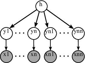
(1-persistent topic model)
Single topic model (): The condition in (9) is always satisfied for the single-topic model, since in this case, and we have
| (10) |
Note that is a diagonal matrix.
Bag-of-words admixture model (): From Lemma 1, the -th order moment of observed variables , for the bag-of-words admixture model (1-persistent topic model), shown in Figure 3, is given by
| (11) |
where is the -th order moment of hidden variables , defined in (3). Note that is a full matrix in general.
Contrasting single topic and bag of words models : Comparing equations (10) and (11), it is seen that the moments under the single topic model in (10) are more “structured” compared to the bag of words model in (11). In (11), we have Kronecker products of the topic-word matrix , while (10) involves Khatri-Rao products of . This forms a crucial criterion in determining of whether overcomplete models are identifiable, as discussed below.
Why persistence helps in identifiability of overcomplete models? For simplicity, let the order of the moment . The equations (10) and (11) reduce to
| (12) | ||||
| (13) |
Note that for the single topic model in (12), the Khatri-Rao product matrix has the same as the number of columns (i.e. the latent dimensionality) of the original matrix , while the number of rows (i.e. the observed dimensionality) is increased. Thus, the Khatri-Rao product “expands” the effect of hidden variables to higher order observed variables, which is the key towards identifying overcomplete models. In other words, the original overcomplete representation becomes determined due to the ‘expansion effect’ of the Khatri-Rao product structure of the higher order observed moments.
On the other hand, in the bag-of-words admixture model in (13), this interesting ‘expansion property’ does not occur, and we have the Kronecker product , in place of the Khatri-Rao products. The Kronecker product operation increases both the number of the columns (i.e. latent dimensionality) and the number of rows (i.e. observed dimensionality), which implies that higher order moments do not help in identifying overcomplete models.
An example is provided in Figure 4 which helps to see how the matrices and behave differently in terms of mapping topics to word tuples.


Note that for the -persistent model, for , the order moment reduces to
| (14) |
Contrasting the above equation with (12) and (13), we find that the -persistent model retains the desirable property of possessing Khatri-Rao products, while being more general than the form for single topic model in (12). This key property enables us to establish identifiability of topic models with finite persistence levels.
4.2 Tensor algebra of the model
In Section 4.1, we provided a representation of the moment forms in the matrix form. We now provide the equivalent tensor representation of the moments. The tensor representation is more compact and transparent, and allows us to compare the topic models under different levels of persistence. We compare the derived tensor form with the well-known Tucker and CP decompositions. We first introduce some tensor notations and definitions.
4.2.1 Tensor notations and definitions
A real-valued order- tensor is a dimensional array , where the -th mode is indexed from to . In this paper, we restrict ourselves to the case that , and simply write . A fiber of a tensor is a vector obtained by fixing all indices of except one, e.g., for , the vector is a fiber.
For a vector , is the -th order diagonal tensor with vector on its diagonal.
The tensor , is stacked as a vector by the operator, defined as
The inverse of operation is denoted by .
For vectors , the tensor outer product operator “” is defined as [41]
| (15) |
The above generated tensor is a rank-1 tensor. The tensor rank is the minimal number of rank-1 tensors into which a tensor can be decomposed. This type of rank is called CP (Candecomp/Parafac) tensor rank in the literature [41].
According to above definitions, for any set of vectors , we have the following pair of equalities:
For any vector , the power notations are also defined as
The second power is usually called the -th order tensor power of vector .
Finally, the Tucker and CP (Candecomp/Parafac) representations are defined as follows [41, 10].
Definition 7 (Tucker representation).
Given a core tensor and inverse factors , the Tucker representation of the -th order tensor is
| (16) |
where denotes the -th column of matrix . The tensor is referred to as the core tensor.
Definition 8 (CP representation).
Given , the CP representation of the -th order tensor is
| (17) |
where denotes the -th column of matrix .
Note that the CP representation is a special case of the Tucker representation when the core tensor is square and diagonal.
4.2.2 Tensor representation of moments under topic model
We now provide a tensor representation of the moments.
For the -persistent topic model, the -th observed moment is denoted by , which is the tensor form of the moment matrix , characterized in Lemma 1. It is given by
| (18) |
where .
This tensor is characterized in the following lemma, and is proved in Appendix A.2.
Lemma 2 (-persistent topic model moment characterization in tensor form).
The -th order moment of words, defined in equation (18), for the -persistent topic model is characterized as 1010 10 The other cases not covered in Lemma 2 are deferred to Appendix A.2. See Remark 12.:
- •
if for some integer , then
(19) where is the core tensor in the above Tucker representation with the sparsity pattern as
where .
- •
If , then
(20)
Comparison with single topic model and bag-of-words admixture model
We now provide the tensor form for the special cases single topic model and bag-of-words admixture model. In order to have a fair comparison, the number of observed variables is fixed to and the persistence level is varied.
CP representation of the single topic model: The -th order moment of the words for the single topic model (infinite-persistent topic model) is provided in equation (20) as
| (21) |
This representation is the symmetric CP representation 1111 11 In Appendix C, we provide a more detailed comparison between our approach and some of the previous identifiability results for the (overcomplete) CP decomposition. of .
Tucker representation of the bag-of-words admixture model: From Lemma 2, the tensor form of the -th order moment of observed variables , for the bag-of-words admixture model (1-persistent topic model) is given by
| (22) |
This representation is the Tucker representation (decomposition) of where the core tensor is the tensor form of the -th order hidden moment , defined in equation (3), and the inverse factors correspond to the population structure .
Comparing the tensor forms for the -persistent topic model (19), single topic model (21), and bag of words admixture model (22), we find that all of them involve Tucker decompositions, where the inverse factors correspond to the topic-word matrix , and the only difference is in the sparsity level of the core tensor . For the bag of words model, with , the core tensor is fully dense in general, while for the single topic model, with , the core tensor is diagonal which reduces to the CP decomposition. For a general topic model with persistence level , the core tensor is in between these two extremes and has structured sparsity. This sparsity property of the core tensor is crucial towards establishing identifiability in the overcomplete regime. The bag-of-words model is not identifiable in the overcomplete regime since the core tensor is fully dense in this case, while an overcomplete -persistent topic model can be identified under certain constraints provided in Section 3, since the core tensor has structured sparsity and symmetry.
5 Proof Techniques and Auxiliary Results
The main identifiability results are given in Theorems 1 and 2 for deterministic and random cases of topic-word graph structures. In this section, we provide a proof sketch of these results, and then, we propose auxiliary results on the existence of perfect -gram matching for random bipartite graphs and a lower bound on the Kruskal rank of random matrices.
5.1 Proof sketch
Summary of relationships among different conditions: To summarize, there exists a hierarchy among the proposed conditions as follows. See Figure 5. First, in the random analysis, the size and the degree conditions 4 and 5 are sufficient for satisfying the perfect -gram matching and the krank conditions 2 and 3, shown by Theorems 3 and 4. Then, these conditions 2 and 3 ensure that the rank and the expansion conditions 6 and 7 hold, shown by Lemma 5. And finally, these conditions 6 and 7 together with non-degeneracy condition 1 conclude the primary identifiability result in Theorem 5. Note that the genericity of is also required for these results to hold.

Primary deterministic analysis in Theorem 5: The deterministic analysis is primarily based on conditions on the -gram matrix ; but since these conditions are opaque (mainly expansion condition on , provided in condition 7), this analysis is related to conditions on matrix itself. See Theorem 5 in Appendix A.1 for the identifiability result based on . We briefly discuss it below for the case when number of words are available under the -persistent topic model. From equation (8), the -th order moment of the observed variables under the -persistent topic model can be written as
| (23) |
The question is whether we can recover , given the . Obviously, the matrix is not identifiable without any further conditions. First, non-degeneracy and rank conditions (conditions 1 and 6) are required. Assuming these two conditions, we have from (23) that
Therefore, the problem of recovering from reduces to finding in .
Then, we show that under the following expansion condition on and the genericity property, matrix is identifiable from . The expansion condition (refer to condition 7 for a more detailed statement), imposes the following property on the bipartite graph 1212
12
denotes all ordered -tuples generated from set which indexes the rows of .,
| (24) |
where is the maximum node degree in set , and the restricted version of -gram matrix, denoted by , is obtained by removing its redundant (identical) rows (see Definition 9). The identifiability claim is proved by showing that the columns of are the sparsest and rank-1 vectors (in the tensor form) in under the expansion condition in (24) and genericity conditions. Note that since we only require expansion on sets larger than Kruskal rank, the expansion condition (24) is a more relaxed condition compared to expansion condition proposed in [7, 43] for identifiability in the undercomplete regime. For a more detailed comparison, refer to Remark 11 in Appendix A.1.
Deterministic analysis in Theorem 1: Expansion and rank conditions in Theorem 5 are imposed on the -gram matrix . According to the generalized matching notions, defined in Section 3.1, sufficient combinatorial conditions on matrix (conditions 2 and 3) are introduced which ensure that the expansion and rank conditions on are satisfied. The following lemma is employed to establish these results, where we state an interesting property which relates the existence of a perfect matching in to the existence of a perfect -gram matching in .
Lemma 3.
If has a perfect -gram matching, then has a perfect matching. In the other direction, if has a perfect matching , then has a perfect -gram matching under the following condition on . All the matching edges should satisfy for all . In words, the matching edges should be connected to nodes in , which are indexed by tuples of distinct indices.
See Appendix A.4 for a proof. Using this lemma, condition 2 implies that has a perfect matching. Then, it is straightforward to argue that the expansion and rank conditions on are satisfied, which is shown in Lemma 5 in Appendix A.3. This leads to the generic identifiability result stated in Theorem 1.
5.2 Analysis of Random Structures
The identifiability result for a random structured matrix is provided in Theorem 2. Sufficient size and degree conditions 4 and 5 on the random matrix are proposed such that the deterministic combinatorial conditions 2 and 3 on are satisfied. The details of these auxiliary results are provided in the following two subsequent sections. In Section 5.2.1, it is proved in Theorem 3 that a random bipartite graph satisfying reasonable size and degree constraints, has a perfect -gram matching (condition 2), whp. Then, a lower bound on the Kruskal rank of a random matrix under size and degree constraints is provided in Theorem 4 in Section 5.2.2, which implies the krank condition 3. Intuitions on why such size and degree conditions are required, are mentioned in Section 3.2 where these conditions are proposed.
5.2.1 Existence of perfect -gram matching for random bipartite graphs
We show in the following theorem that a random bipartite graph satisfying reasonable size and degree constraints, proposed earlier in conditions 4 and 5, has a perfect -gram matching whp.
Theorem 3 (Existence of perfect -gram matching for random bipartite graphs).
Consider a random bipartite graph with nodes on the left side and nodes on the right side, and each node is randomly connected to different nodes in . Let . Assume that it satisfies the size condition (condition 4) for some constant and the degree condition for some constants (lower bound in condition 5). Then, there exists a perfect (-saturating) -gram matching in the random bipartite graph , with probability at least for constants and , specified in (5) and (6).
Note that the sufficient size bound in the above theorem is also necessary (see Remark 3), and is therefore tight.
Remark 10 (Insufficiency of the union bound argument).
It is easier to exploit the union bound arguments to propose random bipartite graphs which have a perfect -gram matching whp. It is proved in Appendix B.1 that if and the size constraint for some is satisfied, then whp, the random bipartite graph has a perfect -gram matching. Comparing this result with ours in Theorem 3, our approach has a better size scaling while the union bound approach has a better degree scaling. The size scaling limitation in the union bound argument makes it unattractive. In order to identify the population structure in the overcomplete regime where , we need access to at least -th order moment under the union bound argument, while only the -th order moment is required under our argument.
5.2.2 Lower bound on the Kruskal rank of random matrices
In the following theorem, a lower bound on the Kruskal rank of a random matrix under dimension and degree constraints is provided, which is proved in Appendix B.1.
Theorem 4 (Lower bound on the Kruskal rank of random matrices).
Consider a random matrix , where for any , there are number of random non-zero entries in column . Let . Assume that it satisfies the size condition (condition 4) for some constant and the degree condition for some constant (lower bound in condition 5) and in addition is generic. Then, , with probability at least for constants and , specified in (5) and (7).
Acknowledgements
The authors acknowledge useful discussions with Sina Jafarpour, Adel Javanmard, Alex Dimakis, Moses Charikar, Sanjeev Arora, Ankur Moitra and Kamalika Chaudhuri. A. Anandkumar is supported in part by Microsoft Faculty Fellowship, NSF Career award CCF-1254106, NSF Award CCF-1219234, ARO Award W911NF-12-1-0404, and ARO YIP Award W911NF-13-1-0084. M. Janzamin is supported by NSF Award CCF-1219234, ARO Award W911NF-12-1-0404 and ARO YIP Award W911NF-13-1-0084.
Appendix A Proof of Deterministic Identifiability Result (Theorem 1)
First, we show the identifiability result under an alternative set of conditions on the -gram matrix, , and then, we show that the conditions of Theorem 1 are sufficient for these conditions to hold.
A.1 Deterministic analysis based on
In this section, the deterministic identifiability result based on conditions on the -gram matrix, , is provided.
In the -gram matrix, , redundant rows exist. If some row of is indexed by -tuple , then another row indexed by any permutation of the tuple has the same entries. Therefore, the number of distinct rows of is at most . In the following definition, we define a non-redundant version of -gram matrix which is restricted to the (potentially) distinct rows.
Definition 9 (Restricted -gram matrix).
For any matrix , restricted -gram matrix , , is defined as the restricted version of -gram matrix , where the redundant rows of are removed, as explained above.
Condition 6 (Rank condition).
The -gram matrix is full column rank.
Condition 7 (Graph expansion).
Let denote the bipartite graph with vertex sets corresponding to the hidden variables (indexing the columns of ) and corresponding to the -th order observed variables (indexing the rows of ) and edge matrix . The bipartite graph satisfies the following expansion property on the restricted version specified by ,
| (25) |
where is the maximum node degree in set .
Remark 11.
The expansion condition for the bag-of-words admixture model is provided in (4), introduced in [7]. The proposed expansion condition in (25) is inherited from (4), with two major modifications. First, the condition is appropriately generalized for our model which involves a graph with edges specified by the -gram matrix, , as stated in (23). Second, the expansion property (4), proposed in [7], needs to be satisfied for all subsets with size , which is a stricter condition than the one proposed here in (25), since we can have .
The deterministic identifiability result based on the conditions on , is stated in the following theorem for , while case is addressed in Remarks 4 and 11. The identifiability result relies on access to the -th order moment of observed variables , defined in equation (2) as
Theorem 5 (Generic identifiability under deterministic conditions on ).
Proof: Define . Then, the moment characterized in equation (23) can be written as . Since both matrices and have full column rank (from conditions 1 and 6), the rank of is where , and furthermore . Let be any basis of satisfying the following two properties:
- 1)
’s have the smallest norms.
- 2)
’s have smallest (tensor) ranks in the -th order tensor form, i.e., , have smallest ranks.
Let the columns of matrix be for . Since all the ’s (which belong to ) are rank-1 in the -th order tensor form (since ) and the number of non-zero entries in each of ’s is at most , we conclude that
| (26) |
The above bounds are concluded from the fact that and therefore the norm and the rank properties of ’s are upper bounds for the corresponding properties of basis vectors ’s (according to the proposed conditions for ’s).
Now, exploiting these observations and also the genericity of and the expansion condition 7, we show that the basis vectors ’s are scaled columns of .
Since for is a vector in the column space of , it can be represented as for some vector .
Equivalently, for any , where is the -th column of matrix and is a scalar which is the -th entry of vector . Then, the tensor form of can be written as
| (27) |
where the last equality is based on the notation defined in Definition 8. We define as the vector which contains only the non-zero entries of , i.e., is the restriction of vector to its support. Therefore, , where . Furthermore, the matrix is defined as the restriction of to its columns corresponding to the support of . Let denote the -th column of . According to these definitions, equation (27) reduces to
| (28) |
which is derived by removing columns of corresponding to the zero entries in .
Next, we rule out that under two cases ( and ), to conclude that ’s vectors are scaled columns of .
Case 1: .
Here, the number of columns of is less than or equal to and therefore it is full column rank. Since, all the components of CP representation in equation (28) are full column rank 1313 13 Note that for , this full rank condition can be relaxed by Kruskal’s condition for uniqueness of CP decomposition [15] and its generalization to higher order tensors [44]. Precisely, instead of saying , it is only required to have to argue the result of case 1. This only improves the constants involved in the final result., for any 1414 14 Note that for , since the (tensor) rank of any vector is 1, this analysis does not work. , we have , which contradicts the fact that in (26).
Case 2: .
Here, we first restrict the -gram matrix to distinct rows, denoted by , as defined in Definition 9. Let . Since is the restricted version of , we have
where the second inequality is from Lemma 4, and the third inequality follows from the graph expansion property (condition 7). This result contradicts the fact that in (26).
From above contradictions, and hence, columns of are the scaled versions of ’s.
The following lemma is useful in the proof of Theorem 5. The result proposed in this lemma is similar to the parameter genericity condition in [7], but generalized for the -gram matrix, . The lemma is proved on lines of the proof of Remark 2.2 in [7].
Lemma 4.
If is generic, then the -gram matrix satisfies the following property with Lebesgue measure one. For any vector with , we have
where for a set , .
Here, we prove the result for the case of . The proof can be easily generalized to larger .
Let be generic, where is an arbitrary matrix, perturbed by random continuous perturbations . Consider the 2-gram matrix . It is shown that the restricted version of , denoted by , satisfies the above genericity condition. We first establish some definitions.
Definition 10.
We call a vector fully dense if all of its entries are non-zero.
Definition 11.
We say a matrix has the Null Space Property (NSP) if its null space does not contain any fully dense vector.
Claim 1.
Fix any with , and set . Let be a submatrix of . Then .
Proof of Claim 1: First, note that can be expanded as
Let and let , where is the -th row of . Also, let and be the corresponding submatrices of and , respectively. For each , denote by the null space of the matrix . Finally let . Then, . We need to show that, with probability one, does not contain any fully dense vector.
If one of does not contain any full dense vector, the result is proved. Suppose that contains some fully dense vector . Since is a submatrix of , every row of contains at least one non-zero entry. Therefore,
where are independent random variables, and moreover, they are independent of and thus of . By assumption on the distribution of the ,
| (29) |
Consequently,
| (30) |
for all . As a result, with probability one, .
Now, we are ready to prove Lemma 4.
Proof of Lemma 4: It follows from Claim 1 that, with probability one, the following event holds: for every , and every submatrix of where , then has the NSP.
Now fix with . Let and . Furthermore, let be the restriction of vector to ; observe that is fully dense. It is clear that , so we need to show that
| (31) |
For the sake of contradiction, suppose that has at most non-zero entries. Since , there is a subset of entries on which is zero. This corresponds to a submatrix of which contains in its null space. It means that this submatrix does not have the NSP, which is a contradiction. Therefore we conclude that must have more than non-zero entries, which finishes the proof.
A.2 Proof of moment characterization lemmata
Remark 12.
In Lemmata 1 and 2, a specific case of order and persistence () was considered. Here, we provide the moment form for a more general case. Assume that for some integers , then
where is the hidden moment as
The tensor form is also characterized as
where is the core tensor in the above Tucker representation with the sparsity pattern as follows. Let . If
we have
Otherwise, .
Proof of Lemma 1: In order to simplify the notation, similar to tensor powers for vectors, the tensor power for a matrix is defined as
| (32) |
First, consider the case for some integer . One advantage of encoding , by basis vectors appears in characterizing the conditional moments. The first order conditional moment of words , in the -persistent topic model can be written as
where . Next, the -th order conditional moment of different views , in the -persistent topic model can be written as
which is derived from the conditional independence relationships among the observations , given topics . Similar to the first order moments, since vectors , are encoded by the basis vectors , the above moment can be written as the following matrix multiplication
| (33) |
where the notation is defined in equation (32). Now for the -th order moment, we have
| (34) |
where results from the independence of and given and is concluded from the independence of and given and the independence of and given . Equation (33) is used in and finally, the -th order moment of is defined as in .
For , we have by the law of total expectation
where the third equality is concluded from the conditional independence of variables , given and the model assumption that . Substituting this in equation (34), finishes the proof for the -persistent topic model. Similarly, the moment of single topic model (infinite persistence) can be also derived.
Proof of Lemma 2: Defining and , the -th order moment of the -persistent topic model proposed in equation (8) can be written as
Let denote the corresponding column of indexed by -tuple . Then, the above matrix equation can be expanded as
where relation is used in the last equality. Let denote the vectorized form of -th order moment . Therefore, we have
Then, we have the following equivalent tensor form for the original model proposed in equation (8)
A.3 Sufficient matching properties for satisfying rank and graph expansion conditions
In the following lemma, it is shown that under a perfect -gram matching and additional genericity and krank conditions, the rank and graph expansion conditions 6 and 7 on , are satisfied.
Lemma 5.
Proof: Let denote the perfect -gram matching of the bipartite graph . From Lemma 3, there exists a perfect matching for the bipartite graph . Denote the corresponding bi-adjacency matrix to the edge set as . Similarly, denotes the corresponding bi-adjacency matrix to the edge set . Note that and .
Since is a perfect matching, it consists of rows, each of which has only one non-zero entry, and furthermore, the non-zero entries are in different columns. Therefore, these rows form linearly independent vectors. Since the row rank and column rank of a matrix are equal, and the number of columns of is , the column rank of is or in other words, is full column rank. Since is generic, from Lemma 6 (with a slight modification in the analysis 1515 15 Lemma 6 result is about the column rank of itself, but here it is about the column rank of for which the same analysis works. Note that the support of (which is full column rank here) is within the support of and therefore Lemma 6 can still be applied.), is also full column rank with Lebesgue measure one (almost surely). This completes the proof of part 1.
Next, the second part is proved. From krank definition, we have
which is concluded from the fact that the corresponding submatrix of specified by should be full column rank. From this inequality, we have
| (35) |
Then, we have
| (36) |
where (35) is used in the second inequality and the last inequality is from krank condition 3.
In the restricted -gram matrix , the number of neighbors for a set , can be bounded as
where the first inequality is due to the fact that the set consists of rows indexed by the following two subsets: -tuples where all the indices are equal and -tuples with distinct indices, i.e., . The former subset is exactly while the size of the latter subset is at least due to the existence of a perfect -gram matching in . The bound (36) is used in the second inequality. Since , the proof of part 2 is also completed.
Remark 13.
The second result of above lemma is similar to the necessity argument of (Hall’s) Theorem 6 for the existence of perfect matching in a bipartite graph, but generalized to the case of perfect -gram matching and with additional krank condition.
A.4 (Auxiliary) lemma
Proof of Lemma 3:
We show that if has a perfect -gram matching, then has a perfect matching. The reverse can be also immediately shown by reversing the discussion and exploiting the additional condition stated in the lemma.
Let denote the edge set of the bipartite graph .
Assume has a perfect -gram matching . For any , let denote the set of neighbors of vertex according to edge set . Since is a perfect -gram matching, for all . It can be immediately concluded from Definition 3 that sets are all distinct, i.e., for any . For any , let denote an arbitrary ordered -tuple generated from the elements of set .
From the definition of -gram matrix, we have for all . Hence, for all which together with the fact that all ’s tuples are distinct, it results that is a perfect matching for .
Lemma 6.
Consider matrix which is generic. Let be such that and the non-zero entries of are the same as the corresponding non-zero entries of . If is full column rank, then is also full column rank, almost surely.
Proof: Since is full column rank, there exists a submatrix of , denoted by , with non-zero determinant, i.e., . Let denote the corresponding submatrix of indexed by the same rows and columns as .
The determinant of is a polynomial in the entries of . Since can be derived from by keeping the corresponding non-zero entries, can be decomposed into two terms as
where the first term corresponds to the monomials for which all the variables (entries of ) are also in and the second term corresponds to the monomials for which at least one variable is not in . The first term is non-zero as stated earlier. Since is generic, the polynomial is non-trivial and therefore its roots have Lebesgue measure zero. It implies that with Lebesgue measure one (almost surely), and hence, it is full (column) rank. Thus, is also full column rank, almost surely.
Proof of Theorem 1: Since conditions 2 and 3 hold and is generic, Lemma 5 can be applied which results that rank condition 6 is satisfied almost surely and expansion condition 7 also holds. Therefore, all the required conditions for Theorem 5 are satisfied almost surely and this completes the proof.
Appendix B Proof of Random Identifiability Result (Theorem 2)
We provide detailed proof of the steps stated in the proof sketch of random result in Section 5.2.
B.1 Proof of existence of perfect -gram matching and Kruskal results
Proof of Theorem 3: Vertex sets and are partitioned, described as follows (see Figure 6). Define . Partition set uniformly at random into sets of (almost) equal size 1616 16 By almost, we mean the maximum difference in the size of partitions is 1 which is always possible., denoted by . Define sets . Furthermore, partition set uniformly at random, hierarchically as follows. First, partition into sets, each with size at most , and denote them by . Next, partition each of these new smaller sets further into sets, each with size at most . Do it iteratively up to steps, where at the end, set is partitioned into sets with size at most . The first two steps are shown in Figure 6.

Proof by induction:
The existence of perfect -gram matching from set to set is proved by an induction argument. Consider one of intermediate sets in the hierarchical partitioning of with size and its further partitioning into sets, each with size , for any . In the induction step, it is shown that if there exists a perfect -gram matching from each of these subsets of with size to , then there exists a perfect -gram matching from the original set with size to set . Specifically, in the last induction step, it is shown that if there exists a perfect -gram matching from each set to set , then there exists a perfect -gram matching from to .
Base case:
Induction step:
Consider different bipartite graphs , by considering sets and and the corresponding subset of edges incident to them. See Figure 7. The induction step is to show that if each of the corresponding bipartite graphs , has a perfect -gram matching, then whp, the original bipartite graph has a perfect -gram matching.


Let us denote the corresponding perfect -gram matching of by . Furthermore, the set of all subsets of with cardinality are denoted by , i.e., includes the sets with elements in the power set 1717
17
The power set of any set is the set of all subsets of . of .
For each set , take the set of all nodes in which are connected to all members of according to the union of matchings . Call this set as the parents of , denoted by .
According to the definition of perfect -gram matching, there is at most one node in each set which is connected to all members of through the matching and therefore, . In addition, note that sets impose a partitioning on set , i.e., each node is exactly included in one set for some . This is because of the perfect -gram matchings considered for sets .
Now, a perfect -gram matching for the original bipartite graph is constructed as follows. For any , consider the set of parents . Create the bipartite graph , where is the subset of edges incident to partitions and . Denote by the minimum degree of nodes in set in the bipartite graph . Applying Lemma 8, we have
| (37) | ||||
where , and the last inequality is concluded from the degree bound .
Furthermore, we have . Now, we can apply Lemma 7 concluding that there exists a perfect matching from to within the bipartite graph , with probability at least . Refer to Figure 7 for a schematic picture. The edges of this perfect matching are combined with the corresponding edges of the existing perfect -gram matchings , to provide incident edges to each node . It is easy to see that this provides a perfect -gram matching from to .
We perform the same steps for all sets to obtain a perfect -gram matching from any to . Finally, according to this construction, the union of all of these matchings is a perfect -gram matching from to . This finishes the proof of induction step. Note that here we analyzed the last induction step where the existence of perfect -gram matching is concluded from the existence of corresponding perfect -gram matchings. The earlier induction steps, where the existence of perfect -gram matching is concluded from the existence of corresponding perfect -gram matchings for any , can be similarly proven.
Probability rate:
We now provide the probability rate of the above events. Let , denote the total number of times that perfect matching result of Lemma 7 is used in step in order to ensure that there exists a perfect -gram matching from corresponding partitions of to set , whp. Let . As earlier, let denote the set of all subsets of with cardinality . We have
According to the construction method of -gram matching from -gram matchings, proposed in the induction step, is the number of times Lemma 7 is used in order to ensure that there exists a perfect -gram matching for each partition on the side. Since at most number of such -gram matchings are proposed in step , the number can be bounded as
| (38) |
Since in the first step, number of perfect matchings needs to exist in the above discussion, we have
where inequality (38) is used in the first inequality and and inequality are exploited in the second inequality.
Since the result of Lemma 7 holds with probability at least and it is assumed that , by applying union bound, we have the existence of perfect -gram matching with probability at least , for .
Furthermore, note that the degree concentration bound in (37) is also used times. Since the bound in (37) holds with probability at least and it is assumed that , this also reduces to the same probability rate.
The coefficient of the above polynomial probability rate is also explicitly computed, saying that the perfect -gram matching exists with probability at least , with
where is a constant satisfying .
Proof of Theorem 4: Let denote the corresponding bipartite graph to matrix where node sets and index the columns and rows of respectively. Therefore, and . Fix some such that . Then
| (39) |
where the bound is used in the second inequality, and the last inequality is concluded from the fact that .
Let denote the event that for any subset with , we have , i.e.,
Then, by the union bound and inequality (39), we have
where the bound is used in the second inequality. For , the above inequality reduces to
where the size condition assumed in the theorem is used in the second inequality with , and the degree condition is exploited in the third inequality. The last inequality is concluded from the geometric series sum formula for large enough .
Then, Lemma 9 can be applied concluding that , with probability at least for constants and as
where is a constant satisfying .
Proof of Remark 10: Consider a random bipartite graph where for each node :
- 1.
Neighbors are picked uniformly at random among all size subsets of .
- 2.
Matching is picked uniformly at random among all size subsets of .
Note that as long as , the distribution of is uniform over all size subsets of .
Fix some pair .
Then
By the union bound,
which is when is constant.
Therefore, if and the size constraint for some is satisfied, then whp, there is no pair of nodes in set with the same random -gram matching. This concludes that the random bipartite graph has a perfect -gram matching whp, under these size and degree conditions.
B.2 (Auxiliary) lemmata
Lemma 7 (Existence of perfect matching for random bipartite graphs).
Consider a random bipartite graph with nodes on the left side and on the right side, and each node is randomly connected to different nodes in set . Let . Assume that it satisfies the size condition for some constant and the degree condition for some constant . Then, there exists a perfect matching in the random bipartite graph with probability at least where .
Proof: From Hall’s theorem (Theorem 6), the existence of perfect matching for a bipartite graph is equivalent to occurrence of the following event
Similar to the analysis in the proof of Theorem 4, it is concluded from union bound
where the bound is used in the second inequality. From the assumed lower bound on the degree and the fact that , we have
where the second inequality is concluded from the geometric series sum formula for large enough , and is a constant satisfying .
Lemma 8 (Degree concentration bound).
Consider a random bipartite graph with and , where each node is randomly connected to different nodes in set . Let be any subset 1818 18 Note that need not to be uniformly chosen and the result is valid for any subset of nodes . of nodes in with size and be a random (uniformly chosen) subset of nodes in with size . Create the new bipartite graph where edge set is the subset of edges in incident to and . Denote the degree of each node within this new bipartite graph by . Let and . Then, if for a non-negative integer , we have
Proof: For any , we have
where the inner term of summation is a hypergeometric distribution with parameters (population size), (number of success states in the population), (number of draws) and is the hypergeometric random variable denoting number of successes. The following tail bound for the hypergeometric distribution is provided [45, 46]
for given by . Note that assumption in the lemma is equivalent to having . Considering the minimum degree, for any , we have
for given by . Substituting from this equation gives the following bound
| (40) |
Finally, applying the union bound, we can prove the result as follows
where the union bound is applied in the first inequality and the second inequality is concluded from (40).
A lower bound on the Kruskal rank of matrix based on a sufficient relaxed expansion property on is provided in the following lemma.
Lemma 9.
If is generic and the bipartite graph satisfies the relaxed 1919 19 There is no term in contrast to the expansion property proposed in condition 7. expansion property for any subset with , then , almost surely.
Before proposing the proof, we state the marriage or Hall’s theorem which gives an equivalent condition for having a perfect matching in a bipartite graph.
Theorem 6 (Hall’s theorem, [47]).
A bipartite graph has -saturating matching if and only if for every subset , the size of the neighbors of is at least as large as , i.e., .
Proof of Lemma 9: Denote the submatrix by , i.e., . Exploiting marriage or Hall’s theorem, it is concluded that the bipartite graph has a perfect matching for any subset such that . Denote by the corresponding matrix to this perfect matching edge set , i.e., keeps the non-zero entries of on edge set and everywhere else, it is zero. Note that the support of is within the support of . According to the definition of perfect matching, the matrix is full column rank. From Lemma 6, it is concluded that is also full column rank almost surely. This is true for any with and , which directly results that , almost surely.
Finally, Theorem 2 is proved by exploiting the random results on the existence of perfect -gram matching and Kruskal rank, provided in Theorems 3 and 4.
Proof of Theorem 2:
We claim that if random conditions 4 and 5 are satisfied, then deterministic conditions 2 and 3 hold whp. Then Theorem 1 can be applied and the proof is done.
From size and degree conditions, Theorem 3 can be applied, which implies that the perfect -gram matching condition 2 is satisfied with probability at least for .
The conditions required for Theorem 4 also hold and by applying this theorem we have the bound , with probability at least.
Combining this inequality with the upper bound on degree in condition 5, we conclude that krank condition 3 is also satisfied whp.
Hence, all the conditions required for Theorem 1 are satisfied with probability at least , where
and this completes the proof.
Appendix C Relationship to CP Decomposition Uniqueness Results
In this section, we provide a more detailed comparison with some uniqueness results of overcomplete CP decomposition. Here, the following CP decomposition for the third order tensor is considered,
| (41) |
where and .
The most important and general uniqueness result of CP, called Kruskal’s condition, is provided in [15], where it is guaranteed that the above CP decomposition is unique if
Since then, several works have analyzed the uniqueness of CP decomposition.
One set of works assume that one of the components, say , is full column rank [18, 17]. it is shown in [18], for generic (fully dense) components and , if and , then the CP decomposition in (41) is generically unique.
Now, we demonstrate how this CP uniqueness result can be adapted to our setting. First, consider the matrix which is obtained by stacking the entries of as
Then, we have
| (42) |
On the other hand, for the 2-persistent topic model with 4 words (), the moment can be written as
for . The following matrix has the same column span of ,
for some full rank matrix .
Our random identifiability result in Theorem 2 provides the uniqueness of and , given , under the size condition and the additional degree condition 5. Note that as discussed in the previous section, this identifiability argument is the same as the unique decomposition of the corresponding tensor.
Thus, in equation (42), by setting and a full rank square matrix , we obtain the -persistent topic model, under consideration in this paper. Thus, the identifiability results of [18] are applicable to our setting, if we assume generic (i.e. fully dense) matrix . However, we incorporate a sparse matrix , and therefore, require different techniques to provide identifiability results. We note that the size bound specified in [18] is comparable to the size bound derived in this paper (for random structured matrices), but we have additional degree considerations for identifiability. Analyzing the regime where the uniqueness conditions of [18] are satisfied under sparsity constraints is an interesting question for future investigation.
References
- [1] Yoshua Bengio, Aaron Courville, and Pascal Vincent. Unsupervised feature learning and deep learning: A review and new perspectives. arXiv preprint arXiv:1206.5538, 2012.
- [2] Michael S. Lewicki, Terrence J. Sejnowski, and Howard Hughes. Learning overcomplete representations. Neural Computation, 12:337–365, 1998.
- [3] André Uschmajew. Local convergence of the alternating least squares algorithm for canonical tensor approximation. SIAM Journal on Matrix Analysis and Applications, 33(2):639–652, 2012.
- [4] David M. Blei, Andrew Y. Ng, and Michael I. Jordan. Latent Dirichlet Allocation. Journal of Machine Learning Research, 3:993–1022, 2003.
- [5] J. K. Pritchard, M. Stephens, and P. Donnelly. Inference of population structure using multilocus genotype data. Genetics, 155:945–959, 2000.
- [6] A. Anandkumar, R. Ge, D. Hsu, S. M. Kakade, and M. Telgarsky. Tensor Methods for Learning Latent Variable Models. Under Review. J. of Machine Learning. Available at arXiv:1210.7559, Oct. 2012.
- [7] A. Anandkumar, D. Hsu, A. Javanmard, and S. M. Kakade. Learning Linear Bayesian Networks with Latent Variables. ArXiv e-prints, September 2012.
- [8] Sanjeev Arora, Rong Ge, Yoni Halpern, David M. Mimno, Ankur Moitra, David Sontag, Yichen Wu, and Michael Zhu. A practical algorithm for topic modeling with provable guarantees. ArXiv 1212.4777, 2012.
- [9] J.B. Kruskal. More factors than subjects, tests and treatments: an indeterminacy theorem for canonical decomposition and individual differences scaling. Psychometrika, 41(3):281–293, 1976.
- [10] Tamara Kolda and Brett Bader. Tensor decompositions and applications. SIREV, 51(3):455–500, 2009.
- [11] Silvia Gandy, Benjamin Recht, and Isao Yamada. Tensor completion and low-n-rank tensor recovery via convex optimization. Inverse Problems, 27(2):025010, 2011.
- [12] Adam Coates, Honglak Lee, and Andrew Y. Ng. An analysis of single-layer networks in unsupervised feature learning. Journal of Machine Learning Research - Proceedings Track, 15:215–223, 2011.
- [13] Quoc V. Le, Alexandre Karpenko, Jiquan Ngiam, and Andrew Y. Ng. ICA with Reconstruction Cost for Efficient Overcomplete Feature Learning. In NIPS, pages 1017–1025, 2011.
- [14] Li Deng and Dong Yu. Deep Learning for Signal and Information Processing. NOW Publishers, 2013.
- [15] J.B. Kruskal. Three-way arrays: Rank and uniqueness of trilinear decompositions, with application to arithmetic complexity and statistics. Linear algebra and its applications, 18(2):95–138, 1977.
- [16] A. Bhaskara, M. Charikar, and A. Vijayaraghavan. Uniqueness of Tensor Decompositions with Applications to Polynomial Identifiability. ArXiv 1304.8087, April 2013.
- [17] Tao Jiang and Nicholas D Sidiropoulos. Kruskal’s permutation lemma and the identification of candecomp/parafac and bilinear models with constant modulus constraints. Signal Processing, IEEE Transactions on, 52(9):2625–2636, 2004.
- [18] Lieven De Lathauwer. A Link between the Canonical Decomposition in Multilinear Algebra and Simultaneous Matrix Diagonalization. SIAM J. Matrix Analysis and Applications, 28(3):642–666, 2006.
- [19] Alwin Stegeman, Jos M.F. Ten Berge, and Lieven De Lathauwer. Sufficient conditions for uniqueness in candecomp/parafac and indscal with random component matrices. Psychometrika, 71(2):219–229, June 2006.
- [20] L. De Lathauwer, J. Castaing, and J.-F Cardoso. Fourth-order cumulant-based blind identification of underdetermined mixtures. IEEE Tran. on Signal Processing, 55:2965–2973, June 2007.
- [21] Luca Chiantini and Giorgio Ottaviani. On generic identifiability of 3-tensors of small rank. SIAM Journal on Matrix Analysis and Applications, 33(3):1018–1037, 2012.
- [22] Cristiano Bocci, Luca Chiantini, and Giorgio Ottaviani. Refined methods for the identifiability of tensors. arXiv preprint arXiv:1303.6915, 2013.
- [23] Luca Chiantini, Massimiliano Mella, and Giorgio Ottaviani. One example of general unidentifiable tensors. arXiv preprint arXiv:1303.6914, 2013.
- [24] E.S. Allman, C. Matias, and J.A. Rhodes. Identifiability of parameters in latent structure models with many observed variables. The Annals of Statistics, 37(6A):3099–3132, 2009.
- [25] Elizabeth S. Allman, John A. Rhodes, and Amelia Taylor. A semialgebraic description of the general markov model on phylogenetic trees. Arxiv preprint arXiv:1212.1200, Dec. 2012.
- [26] Navin Goyal, Santosh Vempala, and Ying Xiao. Fourier pca. ArXiv 1306.5825, 2013.
- [27] Joseph M Landsberg. Tensors: Geometry and applications, volume 128. American Mathematical Soc., 2012.
- [28] A. Anandkumar, D. Hsu, and S.M. Kakade. A Method of Moments for Mixture Models and Hidden Markov Models. In Proc. of Conf. on Learning Theory, June 2012.
- [29] A. Anandkumar, D. P. Foster, D. Hsu, S. M. Kakade, and Y. K. Liu. A Spectral Algorithm for Latent Dirichlet Allocation. In Proc. of Neural Information Processing (NIPS), Dec. 2012.
- [30] A. Anandkumar, R. Ge, D. Hsu, and S. M. Kakade. A Tensor Spectral Approach to Learning Mixed Membership Community Models. In Conference on Learning Theory (COLT), June 2013.
- [31] E. Mossel and S. Roch. Learning nonsingular phylogenies and hidden markov models. The Annals of Applied Probability, 16(2):583–614, 2006.
- [32] J.T. Chang. Full reconstruction of markov models on evolutionary trees: identifiability and consistency. Mathematical Biosciences, 137(1):51–73, 1996.
- [33] Yuval Rabani, Leonard Schulman, and Chaitanya Swamy. Learning mixtures of arbitrary distributions over large discrete domains. arXiv preprint arXiv:1212.1527, 2012.
- [34] Saneev Arora, Rong Ge, and Ankur Moitra. Learning topic models—going beyond svd. In Symposium on Theory of Computing, 2012.
- [35] Daniel A Spielman, Huan Wang, and John Wright. Exact recovery of sparsely-used dictionaries. In Proc. of Conf. on Learning Theory, 2012.
- [36] Kenneth Kreutz-Delgado, Joseph F. Murray, Bhaskar D. Rao, Kjersti Engan, Te-Won Lee, and Terrence J. Sejnowski. Dictionary learning algorithms for sparse representation. Neural Computation, 15:349–396, February 2003.
- [37] B. Rao and K. Kreutz-Delgado. An affine scaling methodology for best basis selection. IEEE Tran. Signal Processing, 47:187–200, January 1999.
- [38] Nishant A. Mehta and Alexander G. Gray. Sparsity-based generalization bounds for predictive sparse coding. In Proc. of the Intl. Conf. on Machine Learning (ICML), Atlanta, USA, June 2013.
- [39] Andreas Maurer, Massimiliano Pontil, and Bernardino Romera-Paredes. Sparse coding for multitask and transfer learning. ArxXiv preprint, abs/1209.0738, 2012.
- [40] Christopher J Hillar and Friedrich T Sommer. Ramsey theory reveals the conditions when sparse coding on subsampled data is unique. arXiv preprint arXiv:1106.3616, 2011.
- [41] G.H. Golub and C.F. Van Loan. Matrix Computations. The Johns Hopkins University Press, Baltimore, Maryland, 2012.
- [42] XuanLong Nguyen. Posterior contraction of the population polytope in finite admixture models. arXiv preprint arXiv:1206.0068, 2012.
- [43] Daniel A. Spielman, Huan Wang, and John Wright. Exact recovery of sparsely-used dictionaries. ArxXiv preprint, abs/1206.5882, 2012.
- [44] Nicholas D. Sidiropoulos and Rasmus Bro. On the uniqueness of multilinear decomposition of N-way arrays. Journal of Chemometrics, 14(3):229–239, 2000.
- [45] V. Chvátal. The tail of the hypergeometric distribution. Discrete Mathematics, 25(3):285–287, 1979.
- [46] Matthew Skala. Hypergeometric tail inequalities: ending the insanity. http://ansuz.sooke.bc.ca/professional/hypergeometric.pdf.
- [47] Philip Hall. On representatives of subsets. J. London Math. Soc., 10(1):26–30, 1935.