Spin State Detection and Manipulation
and Parity Violation in a Single Trapped Ion
Michael Schacht
2000
Physics
\ChairE. Norval FortsonProfessorPhysics
\SignatureBlayne Heckel
\SignatureAurel Bulgac
\signaturepage
\doctorialquoteslip
Atomic Parity Violation provides the rare opportunity of a low energy window into possible new fundamental processes at very high mass scales normally investigated at large high energy accelerators. Precise measurements on atomic systems are currently the most sensitive probes of many kinds of new physics, and complement high energy experiments. Present atomic experiments are beginning to reach their limits of precision due to either sensitivity, systematics or atomic structure uncertainties. An experiment in a single trapped Barium ion can improve on all of these difficulties. This experiment uses methods to precisely manipulate and detect the spin state of a single ion in order to measure a parity induced splitting of the ground state magnetic sublevels in externally applied laser fields. The same methods can be used to provide precise measurements of more conventional atomic structure parameters. Updated and corrected versions of this document are available from the UW Physics Atomic Physics pages, www.phys.washington.edu/groups/atomic.
Chapter 1 Introduction and Motivation
To the casual outside observer, parity violation might seem to be old news. Its discovery was made in the 50’s in nuclear and high energy experiments, and even the first observations in atomic systems are decades old by now. The existence of this chiral asymmetry is well established and well accounted for in the Standard Model, if a little uncomfortably, and in this context there seems little more to be learned, yet Parity Non-Conservation(PNC) continues to be the subject of much attention and effort.
1.1 Parity Violation as a tool
1.1.1 A quest for something new
This idea that the universe is somehow left-handed is still fascinating and a bit strange, and there remain some fascinating loose ends related to its origin and precise structure, but the current interest in Parity Violation is not so much for its own sake, but instead due to more immediately practical motives, as far as anything can be considered practical here. When its effects are accepted and in the end understood, Parity Violation becomes a tool, and in particular a tool for uncovering clues about the current Holy Grail of physics beyond the Standard Model.
Physicists interested in fundamental processes are, in equal measure, never satisfied and easily bored. The Standard Model was introduced in the 60’s and, for the moment, shows no compelling signs of failing, yet for a number of pretty good reasons, physicists are looking for something else. This is not a matter of any real practical deficiencies as much as a certain lack of elegant internal consistency, as in every case Standard Model calculations agree with experimental observations as precisely as anyone has been able to, respectively, calculate and measure them. The single electron g-2 experiment is a favorite example, the measured magnetic moment of the electron is found to agree with calculated predictions using the Standard Model a a part in .
1.1.2 Missing Pieces
Still, there are some nagging rough edges, an embarrassment of adjustable parameters, a mysterious and not yet well characterized Higgs sector that is particularly important as it aspires to explain why particles can and do have mass, a failure to completely account for the lack of anti-matter compared to matter in at least our local universe, and perhaps its most glaring shortcoming: it completely fails to account for gravity and in fact can’t yet even be made to include it in a consistent way. Even the simple lack of processes whose natural energy scales occur between typical electro-weak energies and the characteristic scale of gravity, the Planck mass, make the structure of the Standard Model as a low energy limit depend on some uncomfortably careful fine tuning of parameters.
So motivates the quest for something deeper, something new. It is possible that these difficulties can be addressed from within the Standard Model through currently unexplored or misunderstood pieces, phase transitions, other non-perturbative effects, or more a detailed picture of the Higgs sector. But this is considered to be significantly less likely and, also calling to mind again the physicists short attention span, effort is directed at extensions to the Standard Model. Then in this context, new means anything not explicitly or implicitly already included in the Standard Model, and in the end this can simply be understood as new particles.
1.2 Heavy particles yield small effects
These new particles, should they exist, are probably very heavy, simply because if they weren’t, we probably would already have seen them. They are expected to begin to appear with masses just above the Electro-Weak scale, which is around the mass of the W and Z bosons, about 100 GeV, though experimental limits have strongly excluded the possibility of new particles with masses of much less than about 0.5-1 TeV. This makes finding them particularly challenging since at the relatively low energies at which we live and presently do experiments, the effects of physics at large energy scales is heavily suppressed. This is easily seen even just at tree level, the classical limit.
1.2.1 A tree level understanding
For the exchange of a single heavy particle of mass the matrix element will include a factor of the (renormalized) propagator for this particle and coupling constants for the vertices. When the exchanged momentum is much less than this mass, the propagator becomes independent.
This process becomes important when the denominator of the propagator is small, that is for energies . But for the expected new heavy particles such energies are well above those accessible in most experiments. In this case the amplitude for this process gets smaller quickly as the mass of the exchanged particle is increased. This provides a convenient excuse for the absence of evidence for the existence of either new particles predicted by various possible new theories such as Supersymmetry or SU(5), and even the Higgs boson of the Standard Model. But this is convenient only for the theorist, the experimentalist still faces the challenge of trying to detect these effects and the task is made increasingly difficult as the search continues to higher masses.
1.2.2 Consequences for atoms
For a comparison, atomic structure is determined almost completely by electromagnetism. For this case, the tree level interaction is a photon exchange giving a factor of the photon propagator . Typical energies in atomic systems are around 1eV, so the characteristic size of an effect due to a new heavy particle with mass of about 1TeV seems to be hopelessly small compared to the natural size of an electromagnetic process. With coupling constants presumed to be a similar order,
In heavy atoms there is some relief because it turns out that there are enhancements due to relativistic electrons and nuclear size that increase this considerably.
This would still be very difficult to detect. Even if an experiment was made sufficiently sensitive for a measurement of this precision, and systematic effects could be understood and controlled at this level, simply interpreting the result would require also understanding the background E-M effects to an even higher precision so they could be separated from the effects due to the new particles. This would be several orders of magnitude better than even a g-2 experiment, with a many-body system considerably more complicated than a single electron. Except in a few very simple cases, it is currently a struggle to understand even just electromagnetic effects in atoms to a part in .
1.3 Parity Violation and new physics
In practice, these difficulties would make such effects from possible new particles undetectable if these new processes didn’t also happen to have a fundamentally different character. One difference that can be exploited is parity violation. The idea of parity and parity violation will be developed more fully in later sections, but in the end all that is important is that it is a symmetry that electromagnetic and strong forces conserve exactly and Weak forces violate maximally.
1.3.1 A new signature
Atoms are held together largely by electromagnetism so atomic states have well defined parities. Perturbations from parity violating interactions can then appear as a mixing of opposite parity states. In particular, atomic PNC experiments measure a mixing of and states, on the order of to . In a parity symmetric environment E-M won’t couple these states so any mixing must be attributed solely to the parity violating perturbation. In this way, measuring a parity violating process no longer requires identifying and understanding a background impossibly many orders of magnitude larger as the contribution from e-m effects is exactly zero.
In the same way, just as importantly, the strong force conserves parity. Though not directly involved in binding an electron to a nucleus, the strong force is responsible for the structure of the nucleus itself and is not nearly as easy to deal with as electromagnetism as it effects are largely non-perturbative. A parity violating strong force would result in a chiral nucleus which creates an asymmetric e-m potential for the electron, in turn contributing to parity violating observables. Small corrections due to Weak interactions within the nucleus do exactly that and must be considered when precision increases. This turns out to provide valuable information about nuclear structure. But in the case of effects due to just the strong interactions there is no contribution, because as with electromagnetism, the Strong force conserves parity, and we are saved the trouble of precisely understanding another naturally much larger background that may be even harder to calculate than QED.
1.3.2 The Weak Interaction becomes background
Certainly there are considerable practical difficulties, these will be discussed in endless detail in later sections. Even excluding that, parity violation isn’t a panacea. For searches for new physics, you still don’t get to compare your result to a background of zero since, of course, the Weak sector of the Standard Model also violates parity. The dominant effect in atoms is the neutral current exchange of a single Weak gauge boson between the nucleus and valence electrons. Effects due to new particles will appear as corrections to Weak Standard Model parity violating observables. In this case, however, the Standard Model effects are already very small since, compared to atomic scale energies the masses of the Weak boson are already very large. Then with the same simple tree level estimates the relative sizes of these new effects are given by a ratio of their masses to the already very high energy Weak scale. Again considering coupling constants of similar order,
A measurement of such a parity violating process to 1% is sensitive to new physics at mass scales of about 1 TeV. This sort of precision is much more reasonable and once done, the interpretation becomes far more tractable. This is the real power of studying parity violation. The electromagnetic and strong forces that would otherwise mask these much smaller effects become effectively transparent to them and parity violating effects due to the heavy processes clearly show through unmodified. In this way parity violation becomes a sensitive differential test for possible classes of new physics.
1.4 High energy experiments and new physics
These parity violating effects in atomic systems, while now reasonably big enough to be visible, are still very small and considerable care must be taken in avoiding systematic errors from external perturbations to measure them precisely. In addition, detailed atomic and nuclear structure calculations must be made to interpret them. Meanwhile, much higher energy nuclear or elementary particle experiments might seem to be a more promising direct route to the same information.
1.4.1 Discovery by production
For sufficiently high energies this would certainly be true. As previously noted, a given particles effects will dominate near the pole of its propagator, where the energy scale is equal to the mass of the particle. Perhaps the right way to find new particles is to search for their resonances when they are directly produced at continually higher energies. To find a particle with a mass of about 1 TeV in this way requires an accelerator with a beam energy of about a TeV, in particular a center of momentum energy equal to the new particle mass. Electron-positron () experiment are the easiest to interpret, but such machines, like SLAC are limited to 50 GeV. The proton-antiproton () collider at fermilab does reach 2 TeV, and LEP at CERN will shortly reach 4, but a proton is actually a complicated bag of junk only a very small part of which might carry a large enough fraction of the total proton energy to produce a heavy particle themselves, and the probability for all the parts to collective use their energy to produce a single new heavy particle is unreasonably small. With these energies the event rate for this kind of search is still too small to stand out from the background of other processes and the strategy would really require building accelerators at arbitrarily high energies. This is becoming increasingly difficult, and in any case is not immediately accessible. So all experiments are constrained to work at energies much lower than the expected natural scale of new physics.
1.4.2 Sensitivity at low energies
Energies up to even a few GeV, still below a or resonance, such as in nuclear experiments, are still insufficient for any kind of direct detection. As before, compared to some generic QED or strong process, 1 TeV particle effects are typically smaller by . This is a considerably larger fraction than for atomic systems, but still too small to be untangled from the background, so even in these much higher energy cases a trick like parity violation must be used. Though the parity violating effects in nuclei are significantly larger than in atoms by these sorts of factors, the fraction of that which is due to new heavy physics is the same. Though much larger relative to general QED effects, the parity violating background due to QED is already zero and so nothing is gained. As energies increase this fraction improves, but another sort of difficulty develops. For any kind of direct detection, these QED effects interpreted as background do go down, but they are also really the signal which is to be measured precisely enough to detect the small piece due to new physics. As this small piece becomes a reasonable fraction of the signal, , in colliding beam experiments the entire signal becomes almost undetectably small and impossible to measure precisely due to systematic problems signal/noise constraints. This can be partly avoided in fixed target experiments. In this case the event rate and sensitivity increase significantly compared to a beam target for the same energy and luminosity simply because there are many more particles for the probe beam to interact with in a fixed target than in another beam. The rate is still small compared to typical accelerator experiments so statistics and systematics will still be a challenge. Also the effective interaction energy is less since 100GeV colliding beams give a center of mass energy of 200GeV while yielding only (40 GeV) in the center of mass frame of a fixed target and the same beam. Still this is a promising means of attack, though currently only one experiment intends to use such a strategy.
1.4.3 Sensitivity at the pole
Most experiments avoid these sensitivity problems by looking instead at Weak processes rather than electro-magnetic. At center of mass energies near the mass, the propagator finally becomes large and the Weak interaction dominates. To estimate the relative contribution by TeV scale physics, the previous tree level approach is still valid, but the result is modified slightly. At the pole the propagator becomes , with the decay width of the . This energy is still presumably much less than the mass of any new particle so its propagator can still be taken to be the usual constant and then for any Weak process, not necessarily parity-violating, the appropriate comparison becomes,
This is comparable to the fraction of the contribution of new physics to parity violating processes at lower energies, in fact even slightly less. This difference actually makes atomic PNC experiments, more sensitive to new tree level interactions and able to probe mass scales 5 times higher than in accelerator experiments, sec.2.4equivilant.
In any case there is certainly no advantage here to working at higher energies. This New to Weak relative ratio could be increased by working slightly off resonance, but this also decreases sensitivity to the dominant process and so is counter-productive as it quickly becomes equivilant to the case of mid-range energies previously discussed, you can’t increase sensitivity by lowering your signal. In the end, there is nothing that can compensate for a very small signal from new physics because of working at energies below its mass scale. By studying parity violation at low and mid-range energies the immediate disadvantages of working there, compared to higher energies, are avoided and in effect all energy scales are equally bad when sufficient energy for direct production of new heavy particles is not available.
1.4.4 New particles in radiative corrections
This tree level survey is not a complete picture of possible contributions from new physics. Observable effects can also appear through radiative corrections (fig.1.1).

This is more complicated to analyze, but will be fully developed in section 2.5. These effects can be distilled and described with two general parameters, S and T, conventionally defined to be zero if only Standard Model physics contributes and all these results can be translated into this universal language for comparison and used to check for consistency or discrepancies that might indicate the existence of new physics. Different experiments depend on different linear combinations of these parameters, and sensitivities are similar though higher energy experiments fare a bit better. A 1% measurement of atomic PNC provides a limit on S to about , while the same precision for a typical collider experiment gives S and T to about .
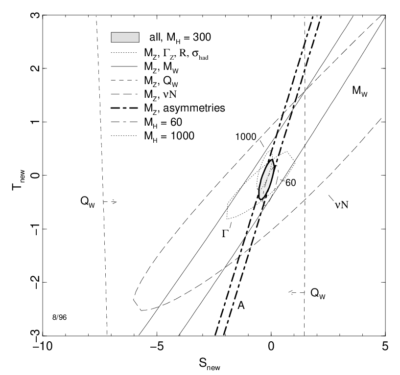
For the moment the global results are consistent with S and T both zero, fig.1.2. Atomic PNC results are beginning to give a case for S negative, but the precision is hardly yet enough to be convincing evidence for new physics.
Again, as in the case of new tree level interactions the results for different experiments are similar and all are about equally sensitive. Higher energy experiments are a little better for radiative corrections, atomic experiments are a little better for new tree level interactions. None is inherently significantly better, so until very high energies can be probed directly all are important for providing constraints and generating new clues, and all complement each other by providing this information at a wide range of energy scales.
To fully appreciate the relative merits of these general classes of measurements, some details of the effects they are intended to detect must be considered. This will be treated explicitly later in sections 2.4 and 2.5. At the least, Atomic PNC provides just yet another constraint, dependent on a different combination of these radiative correction parameters, and more importantly a test of a rather different character since it is at a radically different energy scale. This alone provides considerable merit. An atomic PNC experiment’s increased sensitivity to new tree level interactions, and the possibility that the current trend towards negative S makes an even more compelling case for continued work toward increased precision.
1.5 Atomic PNC
1.5.1 The universal quantity
Precise atomic experiments already exist. The quantity directly measured is a function of the mixing of opposite parity atomic states due to parity violating interactions. For any given set of states this mixing is proportional to a quantity called the weak charge of the nucleus. This is basically the equivilant of the nuclear electric charge in electromagnetism, but in this case for the Weak interaction. So it depends only on the type of atom and is independence of the particular experiment and independent of the set of states used to measure it.
1.5.2 Precision Goals
A Stark interference measurement in Cesium currently provides the most precise result, giving to 0.3%. Prior to that, optical rotation in Thallium gave to 1.2%. These have already provided important information about the Standard Model, in particular constraints on possible new heavy gauge bosons. But as nothing new has yet appeared, even higher precision is required. A useful next target is 0.1%. This would give S to and either resolve the inconsistency with high energy results or provide convincing proof that the discrepancy is real, and along the way be able to uncover new tree level interactions at energy scales up to 2.5TeV.
It is certainly possible that the existing experiments could be improved to this level, but they are probably starting to hit their practical limits in terms of sensitivity and systematics and a new generation of experiments is required. Optical rotation is the method with the highest sensitivity, but the best experiments are now limited by an incomplete knowledge of background, non-parity related rotations, and more importantly, relatively poor atomic theory for the quantities needed to relate the fundamental theories to the direct experimental observables. The overall uncertainly is 1.2% systematics and 2% atomic theory. The background systematics could be better understood with a bit more study, but the theory may tend to prove a tougher challenge as the atoms used in these experiments, Thallium, Lead, Bismuth, have a rather complicated structure with many valence electrons or an easily perturbed core which require more elaborate many-body methods.
In contrast, the Stark interference results with Cs are limited to 0.3% experimental, and 0.6% atomic theory. The atomic structure is relatively simple, being alkali-like it has a single valence electron outside a tightly bound core, so improving the theoretical results should be straight-forward with another round of calculations. Similarly, 7 years of careful study have almost eliminated systematic uncertainties at this level and the sensitivity is rather lower so the experiment is currently limited by statistics.
Better statistics on the Cesium experiment, or a modified version of it, and improved atomic theory could yield the desired 0.1% precision, but currently this is the only experiment with even this chance promise, and even if successful, one result, especially such an anomalous and important result, in a single system, will always be less than completely satisfying. Just as experiments over a large range of energy scales is required for to provide constraints and cross checks from different perspectives and uncover important clues, another, more precise, atomic experiment is required.
1.6 IonPNC
An experiment on a single ion is one possible next-generation project that could address all of the current difficulties and provide this high precision. The Barium IonPNC experiment will measure a light shift due to parity violation that is induced when a particular combination of optical fields is applied, sec.3. This light shift splits the ground state Zeeman sublevels and this energy shift, or equivilantly the ground state precession rate it implies is the measured parity violating observable, fig.1.3.

1.6.1 Improved Systematics
The most readily apparent advantage to this technique is improved systematics. Stark interference experiments use an atomic beam, optical rotation uses an oven of hot vapor. Both are relatively complicated thermal distributions of atoms.
For example, with the high densities and temperatures in ovens, collisions and other interatomic interactions must be considered and accounted for. These can be fiendishly difficult to understand, and exactly those effects are currently limiting the experimental precision of the best optical rotation experiment.
For Stark interference measurements the wide spatial extent of the beam make the uniformity of applied fields very important. Most of the work on systematics is devoted to understanding and controlling the effects of stray and fringing or otherwise nonuniform fields.
The ion parity experiment will use the now well developed techniques of the RF electric quadrupole ion trap. This system, by comparison, is almost trivially simple. Ideally it is just a single isolated particle at rest in free space and this is the fundamental reason for its systematic advantages. Of course, isolated and free is an idealization, an ion trap is not a completely pure environment. The residual perturbations turn out to be largely unimportant in this case but there are complications. In particular, the stability and alignment of the applied optical and magnetic fields is critical 4.4 and, as with any precision experiment, complete enumeration of possible difficulties is elusive. The simple nature of a single ion system, and the small spatial region over which fields must be carefully controlled make the analysis and control of these kinds of systematic errors, if not quite trivial, at least far more tractable.
1.6.2 Sensitivity
This simple feature of a single ion which provides for such advantages in the analysis of systematic errors might seem to, on the other hand, be detrimental, if not catastrophic, for sensitivity. Ovens and vapors are macroscopic collections of atoms and signals are effectively a continuous incoherent average of individual trials for each of some atoms. By comparison, one single ion is an enormous disadvantage. But the same features that ease the systematics can be exploited to gain back the sensitivity.
The size of parity violating effect for any given atom will depend on the strength of the applied fields, in all the cases at hand linearly. Generally a dipole matrix element, , is what is directly measured in the experiment. The size will be given by the mixing , a dipole matrix element, and the amplitude of an applied electric field, , as . Then the size of the electric field controls the size of the effect. Beams and ovens are big, requiring, for example, broad laser beams to fill all the interaction region. In this way field strength is lowered and in the end limited by practical constraints like available, or usable, laser power. A single ion is very small and its orbit in the trap is constrained to regions less than 1. Low power lasers can be focussed very tightly to easily give much higher fields strengths.
If a vapor/beam experiment is regarded as many simultaneous trials, the sensitivity of these and this ion experiment can be discussed in terms of the number of trials, . The precision with which the dipole amplitude can be measured, , generally depends on some line width, , and the number of trials, and possibly some experimental efficiency factor as . The number of trials will be given by the number of atoms, , the total observation time, , and the time it takes to make a single trial, , as , giving
This apparently favors small , but at some point as the trial time is further decreased, the width, , begins to increase. Ideally the linewidth will be determined by some fundamental structural limit giving a finite coherence time so that , but it can also have a contribution from the strength of the interaction used to drive the transition. As the trial time decreased the transition rate must increase so that something observable happens during the trial time. This leads to a transition rate contribution to the width of . When this becomes larger than , begins to increase again like with smaller . Then the uncertainty is minimized for simply, ,
and the precision is limited by the coherence time.
In vapors and beams this coherence time is shortened by collisions and transit times to something less than 1ms. Ion traps are built in ultra-high vacuum systems where pressures reach below torr giving extremely low collision rates. As a result in an ion trap,coherence times are limited only by the natural radiative lifetime of the higher energy state used in the transition. For the states to be used in the barium ion experiment this is a considerable longer 50-80s. Since the ion stays in the same place as long as you care to watch it all of this lifetime is available for observation and there are no transit times or similar limits.
The overall experimental efficiency,, is largely dependent on the design of a particular experiment. Detection efficiency is a measure of how reliably you can tell that something has happened, in this case the something will be a spin transition. Any possible conventional method used to detect this would probably involve looking for a photon emitted either directly by, or as a consequence of this transition. This kind of system would yield very small detection efficiencies, less than about 1/1000 because the photon might not come out in the direction you are looking, and even if it did it might not be seen due to a less than ideal efficiency of a detector, such as with a photo-multiplier tube of 10%. With ion traps, shelving is a common technique that can be used to generate millions of photons corresponding to single transition from another state. This kind of light is easy to detect and with variations of these shelving techniques efficiencies in this experiment will approach 100%. A detailed analysis of this experimental efficiency is considered in sec.6.4.6.
With these experimental conditions the signal to noise ratio is given by,
For the IonPNC experiment in particular, with , this gives, for , with , . This turns out to be comparable to the sensitivity of optical rotation experiments, and larger than the sensitivity for Stark interference measurements, so that an experiment in a single ion should be at least as sensitive as optical rotation. Current ion experiments already yield a S/N of 100:1 for measurements of spin state energy differences. These current results are limited by a large linewidth from sources of magnetic field noise, but the results are completely consistent with this statistical analysis so that this expected S/N for a parity measurement should be realizable with improved technical performance.
1.7 Barium
Besides the general advantages of the ion trap, barium in particular has a number of advantages as the subject of an atomic parity violation experiment. Most importantly, barium is a heavy atom. For an atom with atomic number , the amount of mixing of parity eigenstates is increased by over the earlier first estimate of the natural size of the effect. The mixing would be hopelessly small without this enhancement and so the use of a heavy atom is important. Barium follows cesium in the periodic table and so has a slightly larger amount of mixing, of similar order compared to any other current atomic PNC experiment.
1.7.1 Atomic Structure
Barium is also very like cesium in electronic structure. Singly ionized, barium has a single valence electron outside a tightly bound, 56 electron core. This is identical to the valence configuration of cesium, beyond that the only important difference is an extra proton in the nucleus. This makes for relatively straightforward atomic theory calculations by considering barium to be a single electron system in a coulomb field modified by the charge distribution of the core electrons. The largest part of the calculations are given by considering a static core, but for the precision required for these experiment single, low-level excitations of the core must be included.
Partly for these reasons, the calculations required to connect an atomic parity violation experiment to Standard Model predictions are currently most accurate for cesium. The same techniques can be used for barium and the results should be at least as accurate.
Similarly, radium may be a good choice for future ion parity experiments. It is directly below barium in the periodic table and so has the same more easily calculated electronic structure. It also has a parity violating mixing of atomic states 50 times larger than barium which would yield tremendous improvements in sensitivity. An important practical difficulty is that radium has no stable isotopes, though the longest do last a few days which is plenty long enough to make a parity measurement in this system possible. But for now the associated technical problems largely prevent radium from being the ideal first choice for an ion experiment.
1.7.2 Nuclear Structure and Isotope Comparisons
These precise parity calculations also require detailed knowledge of nuclear properties. Barium also happens to make this task easier. For theory, the hyperfine structure and splitting in isotopes with nonzero nuclear spin make them more difficult to trap and cool. The simplest ion traps will only trap those isotopes with even-even, spin zero nuclei for which the relevant nuclear structure is simpler to calculate.
For quantities which must be determined experimentally, there is a miscellaneous collection of properties that make Barium nuclei good subjects for study. For example, one important bit of knowledge is the nuclear neutron matter distribution. To determine this more precisely at smaller length scales, higher energy probes are needed. In barium these higher energies can be used and still analyzed as much simpler elastic collisions since the excited states turn out to be widely separated from the ground state so that they are not excited even at these energies and as a result don’t contribute to the scattering process.
Finally, with atomic PNC experiments there has always been the desire to do isotope comparisons. In calculating the parity violating mixing of states, atomic and nuclear contributions can be, approximately, factored into an atomic piece that is isotope independent and a nuclear piece that is isotope dependent [Fortson96]. Then, an experiment on many different isotopes can be used to eliminate, or at least reduce, the results dependence on precise atomic structure calculations. The cost is the resulting need for even more precise experimental results and more accurately known nuclear properties. But as the atomic calculations are currently the most difficult to do, and the largest sources of uncertainties in interpreting consequences for the Standard Model, they maybe continue to be the primary difficult in the future and the trade for a possibly easier nuclear structure problem could prove worthwhile.
The barium ion parity experiment is the first in which this kind of comparison would be a practical and promising prospect, in fact is it almost trivial. Different isotopes can easily be loaded, and identified by the ~100MHz scale shifts of their cooling transitions. They already appear regularly during the standard loading procedure, so far at least three different isotopes have been seen. For more systematic future work, specific isotopes can be selected for by adjusting various loading parameters.
The accuracy of this method is improved by studying widely separated isotopes, those having very different numbers of nuclei. Barium has many stable isotopes, those with spin zero nuclei that are most easily trapped range from to giving a very wide range of . This can even be improved to by included those unstable isotopes with lifetimes of a few days that could reasonably though to be used for an experiment. Such a project could be good practice for some future experiment with radium for which, as mentioned, there are no stable isotopes.
1.7.3 Practical Advantages
Barium is a relatively easy ion to trap and as a result is a popular choice for trap studies, in fact it was the first single ion to be trapped. The same practical reasons for this choice still apply and the continued study has made trapping parameters and procedures well established.
Many properties such as energies, lifetimes, isotope shifts and branching ratios, and important effects such as those due to micromotion, magnetic fields and laser polarizations are well known. The frequencies of cooling transitions are visible, where lasers are easily available, and stabilization and locking techniques are abundant and reliable. Sources for neutral barium to ionize and trap exist and ovens and beam methods have already been well developed. Trapping frequencies and voltages are well known and accessible with simple equipment.
None of these pieces make study of a different ion impossible, or even impractical. If barium wasn’t already a good choice for the experiment these practical advantages wouldn’t make it one. Instead all serve to minimize initial practical difficulties and allow for a quicker route to new areas of interest.
1.8 Experiment, Overview, Outline
The primary purpose of this phase of the IonPNC project was to develop the spin state manipulation and detection techniques needed to do an experiment of this kind and determine, and optimize their sensitivity and stability. Effectively determining precisely how such a measurement will be done in practice and how well it can be expected to work. A large part of that, as is the case with any precision measurement, is analyzing systematics, and effort and attention was equally divided between this sort of theoretical analysis and experiment construction and operation.
The following chapters provide a comprehensive summary of the results of these studies and much of the extensive background required to understand their motivation, development and analysis. Here also is an attempt to provide a general understanding of parity violation, and parity violating experiments in general by providing detailed derivations and discussions of the observable consequences of parity violation in atoms starting from the parity violation explicitly wired into The Standard Model. There is a frustratingly large amount of folklore in this field, as there is in any other, details that are commonly known to be true but no-one knows why, or who first noticed it was true. In addition there is extensive recursive referencing such that it is difficult to build the broad background required to fully understand the developments made and the difficulties met in this field and the origin of that understanding is spread among dozens of obscure sources. Here is an attempt to consolidate these results and reduce the recursion depth.
This document fails, however, to be a completely self contained tutorial on parity violation due to size , time and ability constraints. Generally, for results immediately relevant to the experiment are developed in full detail, but for background tropics there are just enough details provided to connect results to familiar result from advanced quantum mechanics, field theory and many-body physics. What is missing is the final details required to connect background results to elementary quantum mechanics and particle theory. These details are largely contained in the separately published IonPNC Operators Manual,[Schacht00]. In addition, only the results that are fundamentally new, or those immediately required for the same new results, are presented here. There are a great many peripheral details, including RF Impedance Matching, Optical Resonating Cavities, Frequency Doubling, Dirac Coulomb Wavefunctions, Many-Body Corrections, Multipole transitions, Alkali like wavefunctions and matrix elements, two state systems and resonance and analysis of other old and new methods for studying parity violation. Some result are necessary for understanding the operation of this particular apparatus, or understanding the many corrections to the conventional analysis, but all are existing and well-known. These details are similarly contained in [Schacht00].
A final omission that must be mentioned is a colloquial discussion of chiral symmetry and parity violation. Understanding the structure and origin of parity violation is not the primary purpose of this project. Instead parity is used as a tool to provide a sensitive probe for the existence of possible new physics. But, the idea of parity violation is interesting enough for its own sake that it deserves some attention. Similarly, to help understand both the parity violating signal and the associated systematic problems of these experiments, it is productive to start to build a more intuitive understanding of this chiral symmetry and the consequences of its conservation or violation in some detail. This includes an elementary discussion of the discrete parity transformation and the ideal of scalars and pseudo-scalars and vectors and axial vectors. For background of this sort, The Ambidextrous Universe by Martin Gardner is highly recommended, as well as The Feynman lectures for certain details of the physical consequences of parity violation.
The most glaring omissions and corrections will be included in a revised version of this thesis available at the IonPNC web site along with the expanded IonPNC Operators Manuals. These are accessible from the links at the University of Washington Physics, Atomic Physics web site, www.phys.washington.edu/groups/atomic/. Currently this groups site is located at www.phys.washington.edu/~fortson. Check there for updated and corrected versions rather than relying on the accuracy of the archived microfilm version.
Chapter 2 Atomic Parity Violation and the Standard Model
The easiest effect to understand of parity violation in atoms, and so far the only one really exploited or carefully studied, is the mixing of opposite parity eigenstates by the tree level exchange of a between a valence electron and the nucleus. On the atomic side, the general structure of this contribution is easily understood with simple perturbation theory, the nonrelativistic Schrodinger equation and a point-like nucleus. For calculations of any accuracy at least some rudimentary relativistic effects and the finite nuclear size must be included, and for precision the full Dirac equation, collective effects of the core electrons and accurate nuclear matter and charge distributions must be included. These improvements will be introduced and outlined but not extensively pursued. There are, for present purposes, a practical difficulty as they provide no insight into new physics. In contrast, the exchange of a single at tree level remains a good approximation to a few percent, but corrections to this will be discussed in considerable details as it is these corrections that contain the desired information about physics beyond the Standard Model. Treating these possibilities carefully provides insight into what kinds of new effects atomic PNC is sensitive to and how they would appear in an experiment.
2.1 Tree Level Overview
A matrix element between arbitrary electronic and nuclear states can be written as a series of Feynman diagrams. The largest contributions are from the tree level exchange of a single particle, which correspond to a classical interaction of fields, fig. 2.1.

2.1.1 Single Particle Interactions
The interaction is simplest when the particle states are plane waves, the matrix element is given immediately by the Feynman rules. For an electron interacting with another point-like fermion, such as a quark, . The currents are given by with and the appropriate coupling constant, . The propagator is given by with .
For Weak currents, for the exchange of a , . The axial coefficient in the vertex is given by the isospin charge . The vector coefficient includes a contribution from the (E+M) charge appearing from the Higgs mechanism used to break the local gauge symmetry, , with given by the weak mixing angle and the coupling constant is , where it turns out that . Also take , .
For atomic wavefunctions the matrix element is best calculated in a spatial basis.The plane wave solutions provide a momentum space basis which can be integrated to get the desired form,
In this basis the propagator is simply a Yukawa field, which for a point particle with unit charge is . The electron wavefunctions vary on length scales of a few Angstroms. In contrast the Yukawa field dies away quickly on length scales of a few thousandths of a fermi, so on atomic length scales the potential is effectively a delta function interaction. Fixing the spatial normalization, , gives the overall amplitude,
The matrix element is then given by a single integral,
This is equivilant to the limit in the momentum basis and accurate to . Errors from this approximation are completely negligible for calculations accurate to .
Low energy effects are conventionally written in terms of the Fermi coupling constant where with . However for comparison with other theories and extensions to the standard model it is useful to use the actual vertex factors so these coefficients will be retained explicitly. It will also be convenient to consider and refer to the vector and axial, parity conserving and parity violating components of the current independently as
where again
2.1.2 Scalar and Pseudoscalar Pieces
Each contains a vector, , a term whose time component is invariants under a parity transformation, a scalar, and whose spatial components change sign, a vector, and axial, contribution, whose time component is a pseudo-scalar, which changes sign under parity, and an axial vector which doesn’t. The diagonal product of either term gives a scalar, an effect invariant under a parity transformation. These will gives effects having a structure identical to electromagnetic processes, a single photon exchange, and so will likely be invisible in comparison as it is heavily suppressed by the mass of the exchanged as discussed in Sec.1. The cross terms give pseudo-scalars, terms that change sign under parity, which give effects that violate parity and will be the interesting terms to consider,
2.1.3 Atomic Matrix Elements
Electron-Nucleon Interactions
This gives transition matrix elements for single particles, but in an atom an electron interacts with a nucleus which is a composite collection of quarks. The conventional picture of the nucleus is that the quarks are bound into nucleons, with characteristic sizes given by , and the nucleons are in turn bound to make the nucleus. For atomic electrons energies are far too low to resolve any of the quark structure of the nuclei, so the quark currents , can immediately be replaced by nucleon currents , given by the coherent sum of the component quark currents. In the end this just results in a of the same structure with axial and vector coefficients given by the sum of the quark coefficients. Since these coefficients are written in terms of and , and a nucleon’s quark content is chosen to get the right and for the nucleon, giving , , . The result still looks like a current for a pointlike particle and none of the composite quark structure appears.
Electron-Nucleus Interactions
The same is less precisely true for the nucleon as a whole. In most of the atom, the electron wavefunction changes appreciably on scales of about an angstrom, which is far longer than the fermi sized length scales of the nucleus,so here a nucleus could be considered approximately as a pointlike particle with the appropriate and , giving , . These can then be identified as the axial and vector weak charge of the nucleus. But near an atoms own nucleus, the wavefunction can change very quickly, for a Dirac electron in a Coulomb field the wavefunction actually diverges at the origin, so that some details of the nuclear structure may be resolved. It turns out that so that nuclear structure details begin to contribute at around the few percent level.
This complicates matters considerably as a nuclear state is generally a complicated multi-particle wavefunction. But for nuclei in particular, the wavefunction can be understood well in terms of a product of independent particle wavefunctions for a well chosen central potential and the end result is that total current becomes just a sum of the currents of all the nucleons, , as given by their single particle wavefunctions so that effectively the nuclear current is given by,
Multiparticle Electron States
Similarly, an atom usually consists of many electrons and an arbitrary state is a multiparticle wavefunction. But for alkali atoms, and alkali-like ions such as Ba+, the system is effectively a single electron bound to a nucleus plus a charge the distribution generated by the remaining core electrons, which can in term be described, as with nuclei, by a product of single particle wavefunctions for this core potential. Different atomic states consist of a changing single particle state for the valence electron and a fixed core and the current is a sum over the currents of the single particle states, as with the nucleus.
Notice that these collective currents contain only contributions from changing one single-particle state, for the electron it is always the valence electron state. This is a result of using considering only a single interaction, a single exchange. It is possible that a core electron could be excited to the new state by the exchange and the valence electron the drop down to replace that core electron. This gives the same final state and so contributes to the total transition amplitude. These processes are slower, the largest effect would be an electro-magnetic decay of the valence electron which is smaller than the single valence electron excitation process by . But this is a contribution above the desired level so precision calculations must include them.
This is the beginning of the complicated atomic theory required for these computations. As mentioned already, these corrections will not be pursued in detail here so this is also where the results presented here will cease to be rigorously accurate and are pursued instead to illustrate the general structure of the effects of the parity violating components of the Weak interaction.
The same corrections would apply to the nuclear currents as well though generally the nuclear state is unchanged between different atomic energy levels except for a change of spin. The spin wavefunctions are more easily dealt with, though for Barium this is irrelevant as its nucleus is spin zero though again that is only true collectively and when including corrections for the non-trivial spatial structure of the nucleus this term may appear again.
2.1.4 Currents and Dirac Matrix Elements
Computing these matrix elements precisely then requires detailed knowledge of the multiparticle wavefunctions, and an even an accurate estimate requires a good set of single-particle wavefunctions for a reasonable effective potential. Their general structure, however, can be understood from a simple expansion of the Dirac wavefunctions in terms of two component spinors.
Scalar Component
is a scalar and can be calculated immediately,
When the initial and final wavefunctions are the same this simplifies further. For example, as discussed above, in general only the spin wavefunctions of a nucleon will change between atomic energy levels so that, in particular the spatial wavefunctions will stay the same. Then requires that the spin wavefunctions also remain unchanged and as a result only identical initial and final nuclear state contribute to this term which can then be written in terms of the proton and neutron charge densities,
If the proton and neutron matter distributions are exactly this same this is further simplified to
For Barium, with , this gives,
There is a similar term for the electron, where appropriate which includes instead the weak charge of the electron, , times the electron charge density . Such a term appears only in hight order corrections to the result being developed here.
2.1.5 Pseudoscalar, Vector and Axial Vector Components
The remaining currents can then be calculated using the appropriate dirac wavefunctions which solve,
The general behavior of the matrix elements by looking at the equations for the two dimensional spinor components of the full four dimensional wavefunction,
Now, for explicit calculations a particular representation for the dirac matrices must be chosen, use,
Substituting these definitions into the Dirac equation gives,
Which simply relates by, in particular,
where is used for shorthand as
This is complicated in practice if is not a simple scalar, but formally the relation will appear the same as the inverse of the operator that appears as the denominator should exist since energies will always be non-zero and in fact positive. Ignoring the possible spin structure of the potential, elementary manipulation of the spin matrices gives,
The matrix elements are seen now in terms of the spin and momentum matrix elements in the more familiar basis of two component spinors.
For this problem it will turn out that much of the motion can be considered to be approximately non-relativistic. In this case the matrix element simplify further. Here so that the lower spinor component of the dirac spinor is much smaller than the upper component which then leads in the usual way to the Non-relativistic wavefunction and the Schrodinger Equations. Rather than start over to get the matrix elements, however, simply take the non-relativistic limits of these Dirac matrix elements with and ,
2.1.6 Non-Relativistic Nuclei
The currents that give the matrix elements contain momentum dependent and momentum independent terms. The momentum dependent terms are generally smaller by a factor or . The nucleus, in particular, is approximately fixed. For hydrogen the electron-nucleus mass ratio is already very small and for heavy atoms such as Barium with the ratio is less than . As a result the nucleus, though not precisely stationary, is certainly moving non-relativistically and its collective motion can be neglected to a part in .
However, even a fixed nucleus ultimately consists of a confined bag of free nucleons, and then quarks, which could be moving, in principle, arbitrarily quickly. It turns out, however, that the nucleon motion is non-relativistic, though not precisely so, . This is a relatively large contribution but it is partially masked by the collective motion of all the nuclei. As mentioned above, electron energies generally aren’t sensitive to sub-nuclear structure and so any momentum-dependent pieces tend to average to zero. The electron matrix elements are partly sensitive to these details at the few percent level and the combination results in partial sensitivity to the motion of the nucleons at about the level.
This is starting to become important, and again a precision calculation will then have to consider them more carefully, but here they will be neglected as the approximation simplifies the matrix elements considerably. Neglecting these term yields, for the nuclear currents,
so that when combined with the electron currents the spatial components in the term involving the axial electron current, and the time component in the term with the vector electron current can be neglected giving,
Again, in the case when the initial and final nucleon wavefunctions are the same the nucleon wavefunctions simplify to,
Note that the former, term, grows with the size of the nucleus, roughly as , the vector contributions of each nucleon to the current add coherently, while the latter term depends on the total spin of the nucleus which is generally much smaller than since nuclear pairing favors nucleons pairs of nucleons with opposite spins and the resulting total nuclear spin tends to be relatively very small. In this way the nuclear spin dependent term is much smaller then the spin independent term, and of course, for spin zero nuclei, such as with Barium, it gives zero.
2.1.7 Non-relativistic Electrons
These two component wavefunctions are more familiar and easier to deal with. For the nucleus they tend to be a good approximation but it is far less accurate for the electrons as it turns out that the electrons become significantly relativistic near the nucleus, which is only apparent when studying the detailed solutions to the dirac equation. Unlike the omissions consider so far, which amount to corrections of a few percent, this modification changes the result by a factor of 2-5. Still the structure is unchanged, and even this non-relativistic case will not be evaluated precisely, so for this survey consider,
A simple single particle solution to the Dirac Equation for a Coulomb potential plus the electron charge distribution and a finite nuclear size provides a reasonable accurate result.
2.2 Parity Mixing
With the nuclear spin dependent term generally smaller than the remaining spin independent term, the largest effect comes from the ,
The parity violating nature of this term is more apparent here in a familiar form. is a vector and is an axial vector so that the dot product is a pseudo-scalar. It changes sign with a parity transformation, changes sign and doesn’t. So that in a left-handed coordinate system an minus sign would have to be included and the form of the equation is not independent of the handedness of the coordinate system. The handedness implicitly defined by this term gives the observable parity violating processes.
2.2.1 Total Spin
Consider an arbitrary pair of initial and final states, and . is a (pseudo)scalar, that is it is invariant under rotation and so commutes with the total angular momentum operators . As a result, it does not change or and so the initial and final total angular momentum must be the same.
2.2.2 Point Nucleus
Further progress now requires details of the nuclear charge distribution and the electron wavefunctions. As discussed above, corrections from the sensitivity of the valence electron to nuclear structure is small, around 1%, so the general structure can be obtained by considering the nucleus to be uniformly distributed, and even more simply, since it is so small relative to atomic dimensions, as a point-like delta function distribution. This results in the matrix element being given by,
The value of the wavefunctions at the origin determine the matrix element. Again, to compute this accurately the full solution to the dirac equation must be used, but again, the general structure can be studied with the much simpler non-relativistic schrodinger equation,
This limit also makes the approximation of a point-like nucleus much better as well but turns out to be poor overall as the solutions to the schrodinger and dirac equations differ considerably near the nucleus.
2.2.3 Angular Momentum
The behavior of the wavefunctions at the origin is particularly easy to understand for the schrodinger equation. For a spherically symmetric spin independent potential, the wavefunction factors the wavefunction into a radial part , an angular part given by a spherical harmonic , and a spin . For any potential satisfying the small dependence of the solutions are given by The matrix element requires a gradient of , so is proportional to,
At this is non-zero only for as this gives independent of , while gives at . In the second factor the first term requires for the same reasons, while the second term is non-zero for and . But an , , wavefunction is spherically symmetric and has zero gradient so only the first term can contribute. The net result is that this term is non-zero only for and , it only couples and states, and again only those having the same .
With , the non-zero matrix elements are then given by,
2.2.4 Size
The overall size of this mixing matrix elements is easy to determine. , and . The must have dimensions of length-3/2 so that a three dimensional spatial integral gives a unitless normalization. The derivative gives another factor of length in the denominator, .
dependence
For the hydrogen atom length scales are around an angstrom, for a simple electron bound to a nucleus with charge the lengths scales are reduced linearly by . So apparently . But for a many electron atom the increase is not that extreme. It turns out that the extra charge results in the electron being more likely to be found near the nucleus, and in particular at the origin, by a single factor of , since far from the nucleus most the of nuclear charge is shielded by the core electrons, but the momentum near the nuclear is still increased by , . With , This yields the estimate,
,
In these units giving
This gives the typical size of the mixing and some insight into its dependence on the charge of the nucleus.
Mixing in Barium
For Barium with this gives,
This is exactly the right order of magnitude. Again an accurate calculation requires at least Dirac wavefunctions and a finite nuclear size.
2.2.5 Phase
Besides the overall size, this explicit calculation results in a purely imaginary matrix element. This turns out to be a general result and can be understood in terms of the parity and time-reversal symmetry of the operator.
Consider any operator with well defined symmetry properties under parity and time reversal,
These properties can be used about matrix elements of between states particular kinds of states,
For parity eigenstates, matrix elements are easily shown to satisfy a simple selection rule,
This is the basis of the usual selection rules. If the product of all the parity quantum numbers is negative, this matrix element must be zero. If is odd the initial and final states must have opposite parity to give a nonzero matrix element, similarly even only couples states of the same parity.
A similar transformation using time reversal leads to a relation of this matrix element to a corresponding matrix element between time reversed states. Time reversal is weird, eventually you can show, Sakuri 4.4.42[SakuraiQM],
Where are the time reversed states, and for angular momentum states,
The time reversal flips the spin of the state. This can be flipped back with a rotation about an axis perpendicular to . For example, as shown in 3.3.2,
This gives
where also happens to be the parity, , of the state. The time reversed matrix element then becomes
If the hamiltonian is also rotationally invariant, as it must be if these angular momentum states are actually eigenstates, the rotation operators leave invariant and yield,
The previously derived parity selection rules show that the matrix element is zero unless or and the matrix element relation can be written more compactly,
Then, if the product of symmetry quantum numbers is odd, the matrix element must be imaginary, and if the product is even, the matrix element must be real.
is odd, as already observed, and, since both vectors change sign with time-reversal, even, any non-zero matrix elements must be purely imaginary, as already seen explicitly in one case. This phase has important consequences for the resulting observables and so will generally be written explicitly for emphasis.
2.2.6 Perturbation Theory
In the end the result is simply a mixing of and states. The effects of this on the atom are simply understood with first order perturbation theory. In the usual way, separate the full hamiltonian into a piece that is easy, which in this case will be taken to include just electromagnetic interactions, , and a piece that is small, here Weak, or possible new non Standard Model interactions, or . The basis for expanding solutions to the full hamiltonian is then the usual atomic states and to first order in the interaction the wavefunctions become,
As just shown the interaction couples and states with the same giving, in particular,
Write the matrix element coefficients in terms of
Since the matrix element is purely imaginary, is real. This gives,
states are similarly modified,
Energy separations in atoms are of order , independent of since much of the wavefunction is outside the nucleus where most of the nuclear charge is shielded, though it of course depends on the ionization. With this observations the general size of the mixing can be determined,
where again for Barium with ,
2.3 Corrections and Additional Effects
This component of the tree level exchange account for all of the mixing to within a few percent. This estimate of the size of the matrix element provides a good measure of the order of magnitude of the mixing. Again, an accurate calculation of this term requires a single particle wavefunction solution to the dirac equation with a finite nuclear size. Precise calculations of the mixing require the nuclear spin dependent terms where appropriate, and eventually the components of the current neglected in the approximation of non-relativistic nucleons. Finally, the many-body effects from the multiple electrons must be included in the initial and final electron states, as well as the nucleon states when the initial and final nuclear states are not the same. Even with these contributions only the tree level exchange has so far been included. Equally important at this level of precision are other processes and Standard Model radiative corrections to this tree level exchange.
2.3.1 Electron-Electron Interactions
A exchange takes place between any two fermions with a weak charge. The interaction considered so far is that between the electrons and the nucleus, electron-electron interactions can also be considered. This is included simply by contracting the Weak electron currents
A similar consideration of the pseudo-scalar pieces of this term, and approximately non-relativistic electrons gives the largest contribution as a term very similar to that identified as the primary contribution to the electron-nucleus exchange,
Here is the core electron mass density, normalized to have unit volume so the includes all the information about the number of electrons, with . This ends up being small just due to atomic structure.
2.3.2 Vertex Renormalization
The structure of either the electron or nucleon vertex is altered by vertex corrections, figure2.2.

A photon in the vertex loop changes the structure of the vertex by , just as the electromagnetic vertex of an electron acquires an anomalous magnetic moment, and both the vector and axial components of the vertex are adjusted slightly. However, the analogous contribution for a gluon in a nucleon vertex on the axial term is relatively very large. This effectively renormalized the axial charge of a nucleon, which has so far appeared only in the nuclear spin dependent term of the tree level exchange, and is included by modifying the weak coupling constant to .
2.3.3 Vertex Renormalization
An additional in the loop adds a contribution where is the mass of the fermion whose vertex is being modified. This is a small correction to the vertex, but it will also modify the vertex, figure 2.3.

The modification to a nucleon’s photon vertex is the largest since it has the largest mass. It effectively gives a small axial component to the photon vertex,
Then a simple photon exchange between an electron and a nucleus contains a pseudo-scalar term. In effect, the nucleus aquires a chiral electro-magnetic current distribution and the electron is no longer bound by a spherically symmetric potential and the same kind of parity mixing occurs. This term involves the axial current of the nucleon, which as pointed out previously is further suppressed by the spin of the nucleus. In nuclei with non-zero spin this amounts to another adjustment to the atomic state parity mixing.
2.4 New Tree Level Physics
The parity violating effects considered so far are those due to Standard Model processes, in particular, the largest effect is given by a single exchange between an atomic electron and the nucleus. Possible extensions to the Standard Model also naturally violate parity and these new processes can alter the size and structure of the resulting atomic observables. New physics can be understood to mean new particles. The effects of new physics can be studied by considering effects of the addition of various kinds of new particles to the electron-nucleus interaction.
2.4.1 General New Tree Level Interactions
The most straight-forward effects to consider are those due to new tree-level exchanges, figure 2.4.
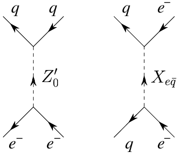
These examples include possible new particles that occur in extended models like or , [CollinsMartinSquires]. These include new ’s similar to the Standard Model and leptoquarks. Additional ’s give contributions with identical structure to the Standard Model exchange, which in the limit of a point nucleus the largest contribution becomes,
The structure of an leptoquark exchange is a little strange since it changes quarks to electrons, it would look something like,
This terms is generally a bit messy, even for a non-relativistic point nucleus there are four pseudo-scalar terms involving matrix elements like,
Other models like Technicolor and Supersymmetry, or contributions from one or more Higgs don’t yet appear because they give no new tree level interactions. Technicolor is intended to account for the Strong interaction so only affect nucleon interactions, new vertices given by Supersymmetry always involve two new super-partners where a tree level exchange is just one particle, and similarly Higgs vertices always involve two Higgs particles. These latter possibilities then appear first only in loops, radiative corrections.
The characteristic sizes of these terms can be used to estimate the sensitivity of a measurement of or to particles with a certain range of masses. New interactions give a contributions of order to an effect of order . If the coupling constants are assumed to be about the same order of magnitude, this is a fractional adjustment of order . For precisions of this gives a mass sensitivity of
As discussed in Sec.1.4.3 at the pole this is generally a correction to a process of order . With a similar precision this gives sensitivities of
These estimates are made assuming the new coupling constants are about the same as the Weak coupling constant . For an arbitrary new interaction the coupling constant could in principle be anything implying that even new particles with smaller masses may not be detectable in this way because the coupling constant is very small. But in consistent extensions to the Standard Model, and especially with Grand Unified Theories there are rigid relations between new and old coupling constants, in part because part of the point of a Grand Unified Theory is to reduce the number of fundamental coupling constants. In general the coupling constants are of the same order of magnitude with freedom for adjustment possible only be changing the structure of the model. Specific predictions for sensitivity to new physics then depends on the detailed structure of the model.
2.5 Radiative Corrections
New processes can also appear as corrections to the tree level Weak exchange through radiative corrections. The possibilities for the addition of a single new particle to the tree level diagram are shown in figure 2.5. These largest single-loop corrections all be from new neutral current exchanges.

These are much more complicated to evaluate as they all involve loops which require careful attention to renormalization details to interpret and generally change the structure of the effects as well. However, it turns out that the largest of these radiative corrections can be accounted for very compactly and result in effects with a structure identical to that the effects already considered due to the Weak interaction, and so can be included by adjusting the parameters of these Weak results. The is a slightly specialized and streamlined version of the methods used in [PeskinTacheuchu].
2.5.1 Oblique Corrections
These modifications can can be divided into direct corrections which include vertex corrections and box diagrams and mass renormalization, and oblique corrections, the vacuum polarizations, which only modify the propagator of the exchanged particle. For modifications to weak processes, the contributions from new heavy particles from the direct corrections turns out to be smaller than those from the oblique corrections by a factor ,where is the mass of the lightest fermion attached to the loop and is in all cases very light relative to the likely mass of a new .
The oblique corrections also happen to be the easiest to consider and can be included simply by modifying the propagator of all the Electro-Weak gauge bosons from their bare, tree level form to a full, renormalized . With only this simple observation, the general structure of the effects of the oblique corrections can be determined without any further details regarding the form of the renormalized propagator. Any Electro-Weak vertex will appear as
Matrix elements will be given by contractions of these current through an appropriate propagator. Omitting explicit Lorentz indices, matrix elements are given by
To determine the modifications to neutral current interaction, adjustments to the entire Weak sector must analyzed which then require considering affection on both and propagators as well. Note also the presence of the rather strange looking which appears to propagate a particle that starts as a and ends as a photon, and vice versa. No bare, tree level interaction gives this sort of mixing, giving,
At tree level, at low energy, the unrenormalized propagator yields , giving the usual form of the low energy Electro-Weak effective Lagrangian. With the , and ,
As usual, if desired, , .
With higher order processes it becomes possible to change a into a in particular consider any fermion loop with a and a attached, fig.2.6.

This gives the first non-zero contribution to . Rather than appearing as an additional term this can be included as a modification to the original form of the matrix element since the Weak neutral current contribution already contains terms like . The possible non-trivial Lorentz structure of the propagators can make this rearrangement a little tricky. This will be remedied with the detailed development of the structure of the full propagator. Schematically the result will take the form,
Already the net effect is becoming apparent. With
the effective interaction takes the same form as the original, tree level interaction with renormalized coupling constants.
2.5.2 Full Propagators and Self Energies
The low energy limit of this result is not immediately apparent. In particular the structure of is not yet known and the explicit form of the diagonal propagators has not been determined. These require the detailed forms of the full propagators.
The oblique corrections are included in the propagator through a self energy . At tree level,
The momentum dependent term in the numerator doesn’t appear in the photon propagator, and at low energies is negligible in the propagator of a massive particle, but this Lorentz structure will not appear explicitly again so it is no extra work to retain it for a more general result. With the addition of the oblique radiative corrections the full propagator is given by
This form can include Standard Model corrections as well as contributions for possible new physics. Both these oblique Standard Model corrections and the previously discussed direct corrections must eventually be included to precisely interpret any experimental result, but neither will be discussed explicitly here. The Standard Model oblique corrections can be included implicitly in the self energies by separately considering contributions from existing Standard Model particles and new particles as .
For massive particles, at low energy this modified propagator becomes,
For the photon, with , the Ward identity requires that so that, as seen below, the photon remains massless.This turns out to yield , where is finite, this gives a low energy limit for the photon propagator of,
Ordinarily, as in the case of the , the self energies are straight-forward to calculate and are given as a sum of all 2- point irreducible diagrams with two external legs, call it . This is easily seen from the simple Dyson equation satisfied by the propagator,
giving,
and so .
For the and the this structure is complicated by the fact that a can change a photon to a while propagating so the full propagator for a , for example, contains terms like as well as the usual . These contributions are a bit tricky to count correctly. Consider simply modifying the Dyson equations with the addition of a likely extra term,
and similarly for the . These give plausible recurrence relations that can be checked by expanding them a few times.
To make these kind of calculations a bit tidier omit the explicit appearance of the ’s that glue the propagators together and write the Dyson equations as,
Expanding the propagator in particular gives,
This gives the desired terms involving sequences of an arbitrary number of and terms, but leaves out any terms with repeated ’s which are surely a valid contribution. This is partly remedied by replacing the middle, bare propagator in the additional term of each Dyson equation with a full propagator,
Expanding this as before it quickly becomes apparent that this set of equations over-counts many contributions. For example, two iterations already gives the term .
The trouble in this case is that since the full propagator contains mixing that has already been included in the full propagator. All that is really needed is a propagator with no additional mixing to a to generate the appropriate intermediate propagators. To that end define a modified propagators, , for the and that don’t include mixing. These are easily defined in terms of the previous . The Dyson equations the same as for the ,
giving usual,
The Dyson equation for the full propagator, in particular, can then be written,
A similar expansion of the recurrence gives,
as desired. The mixing now appears explicitly and the ’s in each term can then be expanded to give the correct full series.
Solving for the full propagator,
This can also be seen from modifying the original candidate for the Dyson equation using as it was originally motivated,
Either form gives the correct expression for the self energy,
with the analogous result for the photon. Substituting for gives
The are the usual irreducible 2-point Green’s Functions.
With these definitions the structure of the off-diagonal propagator can be determined. An expansion of the full propagator should give,
These result again provides the proper result of a massless photon. The Ward identity will also give , as well as as previously discussed, so that . This also yields . It will be convenient to be able to explicitly represent the low energy limit for either case. As before define for and , where generally will be finite. This gives, for ,
so that
Notice that for the propagator the mixing turns out to not contribute to the low energy limit.
2.5.3 Low Energy Effective Theory
With these details about the form of in particular the structure of the interaction with these oblique corrections can be determined more carefully, and more explicitly. Using or as convenient, the interaction becomes
which can finally be written in the form,
The low energy limit can now be taken immediately. is finite, and . Including, for the moment, only the explicit for the photon propagators, the matrix element gives,
This gives the original tree level structure with modified parameters,
where these renormalized couplings are then given by,
The tree level forms of the propagators, , , , again gives the original parameters , . The deviation from these tree level values then contain information about about these oblique corrections. Weak charged current interactions and electromagnetic processes depend only on and respectively, so they can be determined independently by experiment, the -decay constant and , and in that sense are fundamental while the bare independent and are derived quantities. These bare quantities don’t appear here anywhere else so their relation to the corrected values does not need to be considered in detail. Non-trivial observable effects are still available through and and with in particular as an input, neutral current experiments then can be used to constrain and .
This form shows that the low energy effective theory can be completely described in terms of at most four paramaters. It will turn out that not all of these are independent and that in fact only three are needed for any energies up to the Electro-Weak scale. These raw quantities, the 2 point functions at zero energy are not the most convenient form for these parameters as, among other things, they are divergent and any sensible use of them requires regularization and so they become dependent on the renormalization scheme. With a little work these quantities can be re-written in terms of more well defined, renormalization and model independent paramaters that can be used to universally describe the corrections due to contributions from new physics. This can be done in a way that is valid for a wide range of energy scales, [PeskinTacheuchu],[Schacht00], allowing an easy mean of comparing the predictions from the results of many different kinds of experiments, but here the motivation for the definitions of these paramaters will only be sketched from a low energy perspective.
2.5.4
The form of oblique contributions to already appear explicitly. Adjustments to still appear implicitly in terms of the low energy limits of the and propagators. The previous form for these limits of the massive propagators could be used here as
This gives,
with the leading coefficient is just . Now separating contributions from Standard Model processes and new physics, as discussed previously,
For small as these corrections are expected to be, to first order,
This gives as the value given by Standard Model processes times a factor that depends on possible new physics given by the difference in the and 2-point functions.
2.5.5 Mass and Wavefunction Renormalization
This particular form of the correction out to be superficially less convenient. The self energy gives an adjustment to the bare mass that appears in this form of the propagator which yields the physical, observed mass. Generally it is convenient to rewrite the propagator in terms of this physical mass since it is directly accessible by experiment and the bare mass is inherently a derived quantity. This also requires the introduction of an wavefunction renormalization.
Rename this bare mass to distinguish it from the physical mass, . The physical mass is defined by the pole of the propagator, at the denominator of the propagator is zero giving . The propagator then becomes,
with
This gives a propagator with the form of a tree level propagator using the real physical mass with an addition coefficient multiplying the amplitude. This is the wavefunction renormalization, given something like the resulting net change in the probability to find a bare particle in a propagating real particle. In scattering experiments this factor is absorbed in external wavefunctions and partly compensated by the vertex corrections. For this low energy theory they will simply be kept explicitly.
Near the mass pole, or for slowly varying , can instead be written more simply in terms of , with ,
This gives
and
with . This value for the wavefunction renormalization is exact at the mass pole,
for small this becomes simply,
At low energy, the original, exact form of the renormalization is more appropriate,
2.5.6
With this distinction between bare and physical mass the correction to depends on,
Since this is already written just to first order in , the difference between these real and physical masses can be neglected as it is a correction of order ,
The masses that appear are now the real physical masses. This is then conventionally written in terms of an Electro-Weak correction parameter as,
giving,
This provides a means of describing the effects of possible new physical processes on any experiment independent of the particular model of the extension to the Standard Model. for when there is no new physics. This particular form for parameterizing the corrections also turns out to have a great practical benefit because the ultraviolet divergences in a single will cancel in the difference and the result is independent of the any renormalization or regularization scheme that would otherwise be needed.
Standard Model corrections are now sufficiently precisely known that can be calculated accurately enough that contributions from new physics can be detected accurately, though there is still a weak dependence on an unknown Higgs mass. A similar definition of could have been made for as
Then giving
Measuring then requires assuming a Higgs mass to calculate to subtract of the Standard Model contribution. An error in that estimate of the mass of about a factor of 10 changes by about .
2.5.7 Effective Weak Mixing Angle
The structure of the low energy effective interaction gives an easy result for and a natural definition for a parameter to describe the effects of new physics on in a model independent way. The analogous results for are not as straight-forward. The effective weak mixing angle to use a low energy is given by,
The derivatives of the 2 point functions are finite so there sum might be a choice for an additional correction parameter, but that turns out to be cumbersome to use in other experiments. More importantly, like the bare masses in , this is still written in terms of the bare parameter . is not directly measurable but can be derived from the other coupling constants and masses. In particular is given in terms of by,
giving
Here is also a bare parameter, but it is similarly given by,
is conventionally used for these purposes, [PeskinTacheuchu]. Also is used in favor of as it is more accurately known. The can be determined from,
The leading coefficient is used to define . With ,
this then provides and in terms of which can then be used with and to give . This still leads to some gruesome algebra and no natural definition for any other model and renormalization independent Electro-Weak correction parameters.
2.5.8 and
A more natural definition of additional correction paramaters arises from considering the wavefunction renormalization factors, though this leads to a more complicated expression for in terms of these parameters. Near the mass pole the propagator is given by,
The deviation of this propagator from , or the deviation from its Standard Model value is taken to be and can also be used to generally describe contributions to electro-weak processes from new physics.
In this form as the derivative of the self energy it is also finite and so renormalization scheme independent.
In practice is not defined in terms of these factors, but in terms of a modified ,
For the and these are conventionally defined as,
doesn’t appear at all in neutral current processes at it is related to the charged bosons. Generally it is not consider either as it tends to be small. With this the effective Weak mixing angle can now be determined. With some algebra,[Schacht00],
2.5.9 STU results
, and provide an easy means of comparing predictions from the results of any Weak experiment. They are well defined formally in terms of the various 2-point functions but don’t have any immediately obvious physics interpretation. The explicit result for some specific kind of new particles provide some insight into their meaning, [PeskinTacheuchu],[Schacht00].
The contributions to the self energies that determine these parameters will generally include fermions and scalars. For a scalar, such as a Higgs with mass , in the limit , , and are given by,
Where is some reference mass scale.
For a single additional fermion of mass ,
A more natural Standard Model extension will include new pair of fermions in additional doublets. With the particles having masses , with ,
In this latter case, increases with each new doublet by , but changes only if the particle masses are different. This is the origin of the identification of as the isospin conserving parameter, since its contribution is independent of the masses of each particle in a possible new doublet, and the isospin breaking parameter since with exact isospin symmetry giving . In this way is sort of a model independent measure of the existence of some kind of new physics and provides some information about the structure of the addition. Also increases linearly with new particle contributions rather than logarithmically as for the other cases so that the largest contribution to will be from new isospin doublets. This contribution is positive, for small isospin symmetry breaking, and so changes to from possible new physics are generally expected to be positive. Also note that is very much smaller than or as it is suppressed by rather than just .
2.5.10
This analysis gives the effects of oblique corrections to any Weak processes. These processes are accounted for simply by adjusting the tree level coupling constants. The effects on any observable are then similarly easily determined by replacing the tree level parameters with the oblique corrected counterparts. In atomic parity violation, the particle theory details enter through and . As noted, is conventionally measured with charged current process and is taken to be externally defined for these atomic processes and so the only effects to consider explicitly are those contained in . At tree level is given by
The effect of the oblique corrections are to change the overall strength of the interaction from to and altered effective mixing angle . These changes can then be contained in ,
The and can in turn be written in terms of and to provide and easy comparison to the results of other experiments,
For the latter as defined above, and . To first order in and this gives,
For Barium in particular with , ,
A measurement of is effectively insensitive to and provides a constraint on to .This is comparable to the sensitivity available with high energy experiments measuring quantities such as Z and W masses and widths, L/R asymmetries at the pole, and deep inelastic neutrino scattering, though atomic experiments are currently only at precisions of about one percent. Again, the constraints on and from all Weak experiments sensitive to these effects are shown in fig.1.2.
Chapter 3 IonPNC
Information about the Standard Model and new physics, and nuclear structure is contained in the nuclear Weak charge . Atomic theory gives the size of the mixing of a given set a states, , which is largest between and states. The remaining task at hand is to measure . In this, all atomic experiments are conceptually the same. The mixing will yield a nonzero amplitude for a transition previously forbidden by parity conservation. The presence of this transition amplitude is detected, and its strength determines the size of .
Observables generated only by this PNC induced transition amplitude are generally unmeasurably small so that driving another allowed transition is required. But, measuring a correction to an existing process from these effects would require very precise calculuations for interpretation. The ideal arrangement is a differential measurement, driving both processes but measuring an effect that depends only on the difference between the parity violating processes and a parity conserving electromagnetic effect.
3.1 Interference and Linearization
In all current atomic PNC experiments, the parity induced amplitude is an electric dipole transition. For pure electromagnetism the atomic states are parity eigenstates and between two levels with the same parity, an electric dipole transition would not be allowed as a dipole operator has odd parity and so must change the parity of a state. With the Weak interaction, atomic states are only mostly parity eigenstates. With a small amount of an opposite parity state mixed into one of the original states a dipole transition to the other is now possible, fig.3.1.

Keeping the small size of this induced amplitude, and its relatively imaginary phase explicit, this coupling will be written as .
Detecting this transition directly would be more difficult than it needs to be. This transition amplitude is proportional to the mixing, but any observable would involve the square of this amplitude, yielding an effect proportional to . itself is a very small , would be prohibitively miniscule. Instead a second, parity allowed transition is also used, .
For optical rotation experiments an E-M allowed magnetic dipole transition between states of the same parity is used. For Stark Interference experiments the nature of the label finally becomes apparent. A static electric field will also mix states of opposite parity, a Stark shift, and allow an electric dipole transition to the second state.
In either case, the total coupling is then given by . Expanding to first order in , observables will involve,
Taking the square root, again only to ,
Thus the cross term, or interference term, yields an effect linear in . Notice the effect is independent of the overall magnitude of to , and instead depends only on the magnitude of and its phase relative to . The precise structure and effect of this cross term depends on the details of the interaction and in general is slightly complicated by the nontrivial Zeeman structure of the states. But coarsely, optical rotation experiments look for effects given by , and Stark interference measurements, .
3.2 The Light Shift
For the Barium ion, the ground state is and the first excited state is . Parity selection rules forbid an electric dipole transition between these two states. Parity violating interactions mix a small amount of higher energy states into the ground state and through this a transition to the state is allowed. To generate the interference term linear in the mixing, , another coupling between these two states is needed. In this case an electric quadrupole transition is used.
The states are now explicitly spin multiplets and the problem must be treated more generally. For a given set of spin sublevels and the electric dipole and electric quadrupole couplings are given by,
The multipole tensor operators are,
To drive these transitions, the simplest thing to consider is two arbitrary standing waves. One is placed so that the ion is exactly at the standing wave’s antinode, where the gradient of the electric field is always zero, so it drives only the dipole transition. The other is placed so that the ion is at its node, where the amplitude is always zero, this drives only the quadrupole transition. For a real experiment, this arrangement may be less than optimal due to practical difficulties or problems with systematic errors, but in exploring the possibilities it allows the strength of each coupling to be independently controlled and the effect of each easily identified. The general behavior that emerges is not changed by any particular implementation.
3.2.1 Geometry for a Simplified Case
For completely independent standing waves, with arbitrary directions, polarizations and phases, this problem is a bit complicated. There are six states with a possible nonzero coupling between any two spin states from different levels. The choice of a particular field geometry can be well motivated, but that requires some formalism that will be developed later. For now, a primitive idea of what can happen can come from just picking an easy case and blindly working out the consequences. For a first look consider the special case where neither of the states are connected to the same state, in particular suppose that polarizations and directions are chosen so that only transitions are coupled by both the dipole and quadrupole fields.

The effectively factors the problem to two 1+2 state systems which can be solved easily, rather than the entire 2+4 state system, and includes both interactions coupling each pair of states so that they can yield a possibly useful interference term. Initially, and apparently simpler system, a product of two 2-state systems, would come from simply driving instead the transitions. This is reasonable for the dipole field with an appropriate choice of coordinates, but it turns out to put some weird geometric constraints on the quadrupole fields necessary to drive these transitions. These generalities will be discussed in complete detail later, for now the simplest configuration to consider is in fact these two uncoupled state systems resulting from driving only transitions.
The fields that generate this can be determined from the explicit expressions for the spherical form of the tensor operators, but again to build some intuitive understanding of the problem the general behavior of these operators can be considered. For along the angular momentum quantization axis the operator will not change the direction of the angular momentum,
Meanwhile and , which can be written in terms of will change by 1,
Then to get a dipole transition which only drive transitions requires, is some combination of and . To be explicit, let the dipole field define the coordinate system and choose the electric field to be in the direction and the propagation to be along . The dipole standing wave will be taken to have the form .
Similarly for the quadrupole term, the behavior of the matrix element can be understood from the way the coordinate operators successively change the angular momentum,
It is useful to note the particular case of . In terms of the spherical coordinate operators so will only change by 2 and not also 0.
Then the quadrupole fields that give are, , or . For simple plane waves, the former corresponds to , in this case parallel to the dipole light propagation direction, the latter propagates perpendicularly to the dipole light but with the polarization fixed parallel. The easiest case to visualize, though not necessarily to implement, is parallel propagation vectors, the second case will be considered later and gives the same results. Here depart slightly from the strategy of just picking some case, looking up the Clebsch-Gordan coefficients and seeing what happens. There is not yet any reason to fix the polarization direction, in the plane, of the quadrupole field, but it will turn out to be important so allow it to be arbitrary. Also consider it to be fully linearly polarized so that the polarization direction can be taken to be purely real, but allow for an overall arbitrary phase in time relative to the dipole field.
Where is the angle of the polarization relative to the axis so that . This slightly generalized form will start to give some insight and intuitive understanding into what happens and why.
After making the rotating wave approximation, 4.3.1, the harmonic time dependence of the fields can be included instead in the states. Then with these fields, at the position of the ion , the matrix elements reduce to,
and are the amplitudes of the co-rotating terms of the applied field, the counter-rotating terms are discarded by the rotating wave approximation. Generally these are half the magnitude of the real field since the power is equally distributed between the co- and counter-rotating terms. These factors of two will not be explicitly carried around, in favor of defining these amplitudes as just described.
Now some more details of the interaction are handy. Writing the operators and fields in spherical form the Wigner-Eckhart theorem can be used to isolate the dependence into Clebsch-Gordan coefficients. With the summation over polarizations implied,
The angular momentum factors are included for convenience so that the reduced matrix elements are symmetric under the exchange of initial and final states. For general fields the amplitudes for a particular dipole transitions are given by,
and for quadrupole transitions,
The coefficients are the appropriate spherical tensors for this case. With these fields, only the terms are non zero,
For the alternate choice of geometry having , the quadrupole field amplitude is given by,. At with the polarization for the previous case allow the propagation direction the the plane to be arbitrary. This gives the field,
and the amplitude is again
identical to the result for the geometry.
3.2.2 Light Shifts
With these two transitions now suitably driven, consider the observable consequences, in particular the resulting energy shifts in the ground state. With these choices the two ground states are not coupled to each other and the problem factors into two 1+2 state problems. Exactly on resonance, or for , the energy shifts for these states is given by, 4.3.2,
simply a incoherent sum of the effects of each individual coupling to the state. Since the matrix elements coupling the are zero anyways, this can be written more compactly as,
Or with understood to be matrices indexed by the spin states,
With , to linear order in
Recall that in spite of the general appearance of this result, it still requires that no interaction couples both ground states to the same excited state, though the general solution to this problem derived later will have almost the same appearance.
3.2.3 Spin Dependence
Before getting the exact final form, consider the general dependence of the shifts, in particular the symmetry. In the sums over matrix elements in each expression all intermediate states are summed over so the summation variable can be changed to . The matrix form of the shifts contains this transformation compactly,
In turn, the dependence of the matrix elements is easy to understand using these particular fields and a simple symmetry property of the Clebsch-Gordan coefficients,
The dependence is the interesting part here, the others will be fixed for a comparison, so just write this as
Here , so later . This can be done safely since is always in integer in these applications and are both either integer or half integer so that is always an integer and is well defined.
For either matrix element the sum over polarizations can be done in reverse order, as can the sum over in the original expression for the energy shift, since it is just an index. Attending to only the dependence,
for this dipole field the amplitudes are related by a simple sign change.
For the still slightly more general quadrupole fields the amplitudes can be written as,
This may be a bit cumbersome for this introduction, but the generality will be useful for the quadrupole term. The simple cases of , give and , so that for the polarization the quadrupole amplitudes are for same, and for , the amplitudes switch sign. The transformation of the couplings is then
Returning to the energy shifts, the quadrupole shift can be evaluated immediately, keeping the sum over implicit,
For this case, independent of the angle of polarization of the quadrupole field, the shift is the same for both spin states. Call this shift simply since is independent of .
For the cross term, finally explicitly consider the more particular quadrupole fields cases of along or , the quadrupole amplitudes would become,
and the change in the shift is given by,
The denotes a for the case of and for .
For this gives which is a spin independent shift just like that due to the pure quadrupole term but significantly smaller by the factor times a ratio of reduced matrix elements . Somehow measuring this shift to determine to a part in would then require measuring the quadrupole shift to a part in . This is an example of the enormous background from parity allowed interactions that it was hoped would be avoided by considering this cross term. The interference generated a shift linear in , but the structure of this parity induced shift is identical to the quadrupole shift.
Far more interesting is to consider . In this case so that the shifts of the two ground state spin levels are in opposite directions and the total shift will be,
3.2.4 Parity Violation
This finally illustrates the fundamental strategy for making an Atomic Parity Violation measurement using a trapped ion. The spin dependent shift is now of a fundamentally different character than the quadrupole shift which is spin independent and moves these levels together. Systematic errors due to misalignments, polarization impurities and other imperfections can complicate this simple picture and will be discussed extensively in sec:4.4, but at this level the splitting is a differential signal for parity violation, an effect that goes to zero as goes to zero since the quadrupole term, which is parity allowed, doesn’t contribute, so the splitting can then be unambiguously interpreted as due to parity violation.
It is clear that this shift is zero if parity is conserved since the dipole amplitude that generates the shift depend on the parity violating mixing of atomic states. It is not immediately obvious how this result, a spin dependent shift of magnetic sublevels violates parity. This is more easily seen by interpreting the splitting to be instead a precession of the spin, the pictures are equivilant, just as a spin in an external magnetic field can be analyzed statically, by determining the new eigenstates of the hamiltonian with the addition of the applied field and their energies, or dynamically in the basis of the original hamiltonian as a precession of the spin about the applied magnetic field. With this it is clear that a precession of the ion’s spin can be used to define handedness, such as that the precession is clockwise or counterclockwise when view from the source of the applied lasers. The direction of the precession with change sign if the experiment is viewed in a mirror placed parallel to the applied lasers.
Many parity conserving, electro-magnetic processes can generate a spin-dependent shift, but in these cases the fields that give such a shift define a chiral coordinate system. Circularly polarized electric fields split magnetic sublevels and the handedness of the circular polarization can be used to define the handedness of the coordinate systems. Similarly a static magnetic field defines a chiral coordinate system since magnetic field are generated by current loops or magnetic moments in the direction of spins. In these cases a mirror image of the experiment would look like a different physical system, magnetic field in the opposite direction, circularly polarized light of the opposite handedness. Since the direction of the precession also changed sign in the mirror image, nothing about the experiment can be used to define left or right.
The splitting is generated by parity symmetric fields. Both applied lasers propagate in the same direction and polarized the same way. There is no ambiguity about the handedness of the environment, as the applied fields can not be used to define a handedness. A mirror image of the lasers gives the same physical conditions, but the result is still a parity dependent spin precession. Such an experiment can then be used to unambiguously define left. Left and right are somehow intrinsically define in the structure of the Standard Model.
3.3 Spin Flip Symmetries
The potential for a spin dependent shift due to the cross term comes from the difference in the spin flip symmetry of the matrix elements, one of the quadrupole or dipole matrix elements changes sign, and the other doesn’t. The quadrupole shift involves the quadrupole coupling twice so the possible sign changes cancel and the shift is spin independent. The PNC term involves a dipole term and a quadrupole term. If fields are chosen so that both amplitudes driving these transitions either do or don’t also change sign, the entire coupling changes sign and the results is a splitting of spin state energies which can be easily distinguished from the quadrupole shift by its spin dependence.
The result is straightforward and easy to understand, but the analysis was a bit abstract. It involved the plausible, put possibly mysterious spin flip symmetry properties of the Clebsch-Gordan coefficients, and the behavior, under the same, of the spherical tensor amplitudes, which are themselves less than intuitive compared to simple cartesian vectors. The former can be understood easily by considering instead the spin flip symmetry of the states, (Sec.Clebsch-Gordan Relations), and the latter avoided by returning to a cartesian basis.
The preference for a cartesian basis for this problem is also a practical advantage rather than just a philosophical bias. The couplings are given by the sum of the products of matrix elements and field amplitudes over all polarization and propagation components. These fields have been chosen to be linearly polarized so that with a proper chose of coordinates, this sum can be given by a single term in a cartesian basis so that the relationship between couplings is given easily by the relationship between the possible terms in the sum. At the same time, linear polarization requires that at least two spherical tensor amplitudes are non zero, for example , gives , , and the coupling requires a sum over many terms which may change differently when spins are flipping making the relationships between entire couplings less transparent. If the fields were chosen so that only one particular spherical tensor amplitude was nonzero, the sum giving the coupling in a spherical basis would require only one term, while the same result using a cartesian basis would require many terms, again for example , requires , . In addition the states are conventionally indexed in terms of a spherical basis and it will be convenient later to consider mechanisms for restricting the interactions to specific subsets of state, independent of polarization, so that a spherical basis again becomes the more natural choice. So it is valuable to construct tools for use in either basis.
Finally, the entire discussion of these spin flip symmetries can be cast in terms of parity transformations and so return the problem full circle to its origin. In addition, this spherical tensor analysis is somewhat cumbersome and must be repeated endlessly when considering systematic errors. When some simple properties of the matrix elements and operators under rotations or reflections are understood, the general structure and origin of the PNC signal and perturbative systematic problems are evident by inspection.
3.3.1 Transformed States
The overall coupling for either transition is given by,
The mechanical method for computing this was just presented, the Wigner-Eckhart Theorem is invoked to write the dependence in terms of Clebsch-Gordan coefficients and the spin flip symmetry then comes from those coefficients,
Now instead, consider transforming the states in the defining expression,
This kind of transformation was considered when deriving the phase of the mixing matrix element, sec.2.2.5. In that case time reversal was used to flip the spin. But time reversal is weird and parity is the general topic, so try to construct some other transformation to flip the spin,
Also just consider unitary representations of the spin flip operator, , so that amplitude of the states are preserved,
In this case the constant of proportionality must be just a phase and will depend on the particular transformation used to represent the spin flip.
It will turn out that, for this particular problem, only this property of unitarity will be required in considering the action of a spin flip operation on a state. The action of the spin flip on an operator, however, will always be important, and when later considering off diagonal elements of these matrix products of the coupling the detailed transformation of the states must be known, so particular representations of a spin flip must be considered. Also in briefly considering the particular effects of these representations on states, some insight is gained into their workings and, as a by-product, provides an easy means of deriving the spin flip symmetry of the Clebsch-Gordan coefficients that was used above.
3.3.2 Geometrical Representations
As already noted, parity itself doesn’t change spin orientations as a spin is an axial vector, but the geometric explanation for this reveals the pieces that can be used to flip spin. Recall the parity transformation can be understood as a mirror reflection, , followed by a rotation by , . The axis of rotation is the vector that was first reflected so that When the direction is a unit vector it is easily seen that the reflection changes the sign of one of the coordinates and the rotation changes the signs of the other two.
With this axis in the directions, neither operation changes the spin, looking down at the plane a counter-clockwise rotation about the axis remains counter-clockwise after a reflection of the axis, so spin up remains spin up, the rotation about the axis similarly doesn’t change the spin orientation. With the transformation axis perpendicular to , anywhere in the plane, the mirror reversal changes counter-clockwise to clockwise, spin up to spin down, and the rotation reorients to again point up.
Both cases illustrate how the total parity transformation preserves spin orientation and the latter suggests two operations that can be used to flip spin giving the possible representations
or
where is contained in the plane. The mirror reflection is more consistent with the spirit of parity, but the rotation is more straightforward to implement so the action of both on angular momentum states and coordinate operators will be considered. Either representation could be picked, along with a particular choice of orientation axis, and the initial analysis simplified, but for various particular calculations the variety will be convenient and by keeping thing general the representation independence of the results will be apparent explicitly.
Spatial Wavefuntions
A general angular momentum state is a combination of orbital angular momentum and spin. To rigorously determine the transformation of a total angular momentum state, the behavior of both pieces must be considered. The action of the rotation and mirror reflection operations on spatial wavefunctions is the easiest to obtain as they are immediate consequences of the transformation of the coordinate operators which are easily understood geometrically. For a given angular momentum and orientation , the angular part of the wavefunction is given by a Spherical Harmonic that is a Legendre polynomial, a phase and a real normalization coefficient,
The Spherical Harmonics have the symmetry,
or
and
The reflection of the direction leaves unchanged, but a rotation about the same axis results in or so that . The transformation of can also be worked out geometrically, with be the angle of in the plane relative to the axis,
For the particular cases of where this gives,
With , and , , , this yields the correct transformations,
With the action of these operators on the coordinates established, the transformation of the wavefunctions follow easily.
For the mirror reflection , and there is no from changing the sign of ,
Then the states transform as,
Note that this is consistent with the usual result for parity,
For completeness, also consider . takes , or and . gives , so that and . For the states,
yielding the same correct result for parity,
Since the mirror and rotation representations of the spin flip are related through the parity transformation, which is that is reflected in the very similar results of each transformation, differing only by the sign in all cases which is the parity of the state , the results for any representation can be written in a more compact form by defining to be the contribution to the parity of the state with angular momentum given by the transformation . For these spatial wavefunctions, , . With this, the results can be summarized nicely as,
In this form a parity transformation looks like,
which requires for consistency, which is satisfied in this simple case.
Clearly these representations of are unitary, as desired. Also, in this case, the phase is linear in so that,
and so and , so when acting on spatial wavefunctions is hermitian.
Spin Wavefuntions
Spins should behave in the same way, angular momentum is angular momentum, but it isn’t immediately clear which branch to use in for as now and are half integer. It is important to get the phases of all the transformations exactly right as they combine to get the sign change this whole analysis is meant to determine, so the careful attention to phase is not merely pedantic. For example, expressions like appear. For integer valued and this product is perfectly well defined as . For either a half integer, each root could be represented as giving a result of , For , half integer this is an ambiguous result as .
For Barium, the spin angular momentum will be a single electron, so strictly only spin 1/2 needs to be considered for this application, but the general case is not too hard to deal with, with a bit a formalism, and the results provide an easy derivation for the spin flip symmetry of the Clebsch-Gordan Coefficients.
Rotations can be dealt with mechanically with the usual rotation matrices, . For rotations about the axis, the results are trivial since is diagonal,
this gives,
This is identical to the result for orbital angular momentum for and integer, and identifies the proper branch to use, , for an odd half-integer.
For rotations about an axis in the plane are more difficulty as exponentiating is non-trivial. Here Wigner’s closed form solution for arbitrary rotations about the axis can be used,
The sum over is for all that doesn’t give a negative argument for a factorial in the denominator. For , this has a particularly simple form. In this case , . Each term in the sum is zero unless the exponent of the term is zero, or and at most only one term contributes to the sum,
This term only contributes to the original sum if none of the arguments of the factorial in the denominator are negative. Consider the terms involving in the denominator,
The sum is over all giving no negative arguments for the factorial in the denominators, but these arguments will be when the factor is also non-zero. These arguments can both be non-negative only when they are both zero, requiring , only the terms that flip the spin are non-zero. For this case and the rotation matrix elements are,
A rotation about an arbitrary axis in the plane, defined by the same as above, can be done by a composition of rotations, first rotate to the axis, , followed by the rotation about the axis given above, , and a final rotation back to the original orientation of axis, . Again the rotations are trivial and the composition gives,
Here some care must be taken in combining the phases. For any , is an integer and is well defined, can also be written as but the branch to use for an odd half integer is not obvious in this form as if could be interpreted as . To simplify this without ambiguity write the real, sign only, phase as , then the phases combine uniquely to give . With the other choice of representation for the sign, the total phase would give and the resulting can’t be unambiguously simplified to as it is not clear whether this should be for an odd half integer, the former path shows that it should be .
With the phase now well defined for all . The transformations of a spin state again corresponds to that for orbital angular momentum, as it should since angular momentum states are defined so that they transform like spherical harmonics, for ,
As for the case of orbital angular momentum, the transformed state is modified by at a most a phase and is unitary, as is also apparent from the original form of the rotation operator. In this case, and the phase is 1 only for an integer and is not, in general, hermitian. This can be written in terms of the previously defined with the modification which gives for and integer as before,
The complementary results for a spin flip based on a mirror reflection are less straight forward. The desired action on the states is clear, the expectation value of some component of the spin should change sign,
this requires
and all perpendicular components should be unchanged. In particular consider , the transformation requires,
It is easy to show that for at least spin 1/2 representations no such operator is possible. must be unitary, so it can be written as where then is hermitian. For the only hermitian operators are , as the algebra quickly closes since . So can only be written as which is a rotation. A mirror reflection is a discrete operation not continuously connected to any three dimensional rotation so can’t be and these are the only possible unitary matrices for so there can be no representation for a mirror reflection.
It is possible that for higher spins there is enough freedom to construct a spin flip operator since products like are not independent of and , but the procedure is far from straightforward and completely dependent on a particular representation. It is also possible that this could be done systematically in more spatial dimensions. A rotation by always changes the sign of two coordinates, if one of the coordinates is always a fourth spatial , the result looks like a reflection in three dimensions. This is each to implement with the coordinate operators with an representation, but the resulting action of such rotations on the angular momentum states isn’t as trivial. This is now getting hopelessly pedantic, though such a strategy will probably be pursued.
The actions of a mirror reflection could be deduced from the action of the rotations and parity from except that the parity operator is also not well, or uniquely, defined. For Dirac 4-component wave functions a parity operator can be constructed but it allows for parity eigenvalues of . In the end only the relative parity of elementary particles are important and assignments are made by convention, defines . The given phase by a mirror reflection can then be determined through
implying , where giving . For an orbital angular momentum wavefunction where this would give as before. This not completely defined phase from the unknown parity of a spin wavefunction will not cause any trouble as will always appear in complementary pairs in any physical quantity that is computed for these atomic calculations and .
Clebsch-Gordan Coefficients
The action of any of these spin flip operators is now well defined for any angular momentum state and they can be immediately used to demonstrate a useful spin flip symmetry of the Clebsch-Gordan coefficients. The Clebsch-Gordan coefficients give the transformation of a direct product of two angular momentum wavefunctions to a combined total angular momentum state, ,
Flipping the spin of each state, and invoking the unitarity of the spin flip,
Now for simplicity pick so that and the entire product of ’s is . The Clebsch-Gordan coefficient is zero expect for so the dependent part of the phase never contributes to a non-trivial coefficient. The triangle selection rule requires that where can differ by integer values from its largest and smallest possible values. This requires that if both and are integer or half integer, must be an integer, while if only one of is half integer, is also half integer. Then at most two of are half integer values, and never only one so is always an integer and the dependent phase can be simplified , finally yielding,
The result should be independent of the representation used, and this rotational spin flip has trivial , though it is a bit mysterious how this holds for where . This gives . The product of intrinsic parities could apparently be anything and if negative this implies that the corresponding Clebsch-Gordan coefficient is zero because it would require that both .
As an example, consider orbital angular momentum states where all the are integers. For this case which gives so that the Clebsch-Gordan coefficient is independent of the sign of the spin directions. At the same time the first relation derived using rotations still holds so consistency requires , which is the same as the requirements on the parity since . For this example, this condition is satisfied. For a multipole transition between states, the parity of the initial state is changed by the parity of the transition so that the only possible final states that give non-zero matrix elements have the parity of the product of the parities of the initial state and the transition. It is easy to show explicitly with the wavefunctions and operators that dipole transitions only couple states of opposite parity, quadrupole transitions couple states of the same parity.
Considering these many general representation of the spin flip operator then yields the desired relation for the Clebsch-Gordan coefficients as well as a statement about transitions and couplings. Rather than a contradiction, this constraint on the product of parities actually generates the usual parity selection rules, but now quite generally for any angular momentum states,
or, since , a more natural representation,
Total Wavefuntions
With the transformation of the Clebsch-Gordan coefficients determined, the action of the total wavefunction under such spin flips can be determined. Total angular momentum includes contributions from orbital angular momentum and spin angular momentum,
Both were shown to transform identically so the total angular momentum state should transform the same way as is easily shown,
The Clebsch-Gordan coefficient is non-zero only for so that dependence in the phase can be factored out of the sum, and the previous spin flip transformation of the Clebsch-Gordan coefficient used to do the sum,
The form of the transformation is identical. This finally shows that for any angular momentum state,
where . For rotations, , this becomes , the phases can be combined unambiguously in complex exponential form, just as for a pure spin state. Similarly for reflections, so that , again combine the phases in complex exponential form but here use so that , of course just the complex conjugate of the previous result. This gives which implies that consistent with the parity selection rules derived immediately above.
3.3.3 Operators
To determine the action on matrix elements, the transformation of the coordinate operators must also be determined. This is easily done from the transformation of the azimuthal angle already determined,
This gives the transformation of trivially. For and ,
For mirror reflections just take which just changes the signs of all the coefficients so that for either representation, the results can be written using which is given, for an integer, by , and for these spatial operators ,
For completeness, also consider , this doesn’t flip spin, but for compactness call it anyways,
The transformation of the spherical tensors can then be determined. For the dipole operators
The transformations give,
The mirror just gives minus this result,
Finally this can be used to quickly get the transformations of the spherical quadrupole operators,
from the transformation of the dipole operators,
Notice the spherical quadrupole operators don’t notice the difference between the mirror reflection and rotation representations of a spin flip.
This generality in the azimuthal angle of the rotation for reflection direction isn’t particularly useful for the immediate purposes of studying the parity light shift matrix elements, but they will prove useful later when exploited to implement other transformations and demonstrate other symmetries. For example, notice that for , just exchanges and coordinates, allowing for an easy means of relating and matrix elements.
The transformation of the all the spherical operators can be written very compactly,
looking very much like the transformation of states,
Where again and for the states, and simplifies to , for operators. (Notation is little loose, is a label as much as it is and index or argument.)
3.3.4 Matrix Elements of Spherical Operators
These compact results make it very easy to finally determine the spin flip properties of couplings,
through the spin flip properties of the matrix elements, with and integers,
This result should be independent of the representation used for , so in particular is should be independent of the which appears explicitly in an overall phase. Consistency then requires that either the entire result is zero, or the phase is zero independent of because or . This gives the usual selection rules. For the rest of the coefficients pick various particular representations for . Using gives , for this application and are both integer or half integer so the is an integer and the product of ’s gives reproducing the result obtained from the Wigner-Eckhart theorem and the spin flip transformation of the Clebsch-Gordan coefficients. For , . Constancy then requires yielding the selection rule, which becomes the familiar parity selection rule,
When considering the composition of these states with . The is the same for both states so that and requiring .
The entire coupling then changes to,
The are generally independent, but their structures are related in a way that allow further simplification. These amplitudes are constructed out of a symmetric piece, , that is the same for both and and anti symmetric piece that changes sign with , , as
For general this can be written,
Dropping the explicit absolute values in the symmetric and antisymmetric parameters, and understanding them to be implied in this context so that is not distinct from , the original and spin flipped couplings are given by,
For arbitrary fields, these parts of the field amplitudes are given by,
and
3.3.5 Matrix Elements of Cartesian Operators
This form isn’t any more practically useful than the corresponding transformation of the Clebsch-Gordan coefficient because the transformation changed the operator. The spin flipped matrix element is related to a matrix element of a different operator. To the determine the behavior of the entire coupling then requires that the field amplitudes and their transformations are also known. A more insightful picture would emerge if the transformation that changed the state, left the operator invariant. This can be done by returning to cartesian coordinates.
With , , ,
Matrix elements of and operators are simply related to the spin flipped matrix element of the same operator, and and transform the same up to a relative sign.
This demonstrates this tidy result in way that is independent of the representation used to the spin flip operator, but still requires the use of the spherical tensors, and an intuitive understanding of this simple result is slightly obscured. By picking a few particular spin flip representations a simple geometric picture emerges and the derivation completely avoids a spherical basis.
For , or , the cartesian coordinate operators transform very simply,
For these transformations, the coordinate operators change by, at most, a sign and it becomes trivial to see that the spin flipped matrix elements involve the same operator, because the transformation doesn’t change the operator. Repeating the calculation of the spin flipped matrix elements using cartesian coordinates,
If is now restricted to or , the transformation is,
the matrix element simplifies to,
For , the dependent phases are all zero, for , , and . For consistency, requires odd. These two cases can also restrict to , the general transformation would yield the complete familiar selection rules as they appeared when considering the matrix elements of the spherical tensors.
For the product of coefficients, gives the same result as from writing these cartesian operators in terms of their spherical tensor counterparts,
As usual, using gives the same results if the parity selection rules are satisfied.
This path completely avoids the spherical tensor operators and, as one result, make it trivial to extend to higher order operators. In particular, quadrupole operators will get another , use , and the final sign just depends on the numbers of coordinates, , used in the operator,
Obviously this trivially extends to matrix elements of products of any number of coordinates,
3.3.6 Products of Matrix Elements and Selection Rules
The intended immediate application of the transformations constructed here is to be able to quickly, intuitively evaluate the spin flip properties of various energy shifts. These shifts are the sums of diagonal elements of products of coupling matrices like
where a particular coupling is given in a spherical basis by
and in a cartesian basis will involve terms like
with . For the parity experiment,
For these sorts of quantities, some of the generality considered, the action of an arbitrary spin flip on a state, becomes moot. For the states, the most important property of a spin flip operator is that it is unitary, so that the amplitude of the transformed state differs by at most a phase, . In the shifts, both of the states involved appear once each as initial and final states so that these possible phases introduced by a particular spin flip operator exactly cancel. Implicitly summing over the intermediate spin orientations ,
The transformation symmetries apply term by term to each matrix element, so the sum over , and even need not be done for these expressions to hold, except for the initial changing the sign of as a summation index, so it it generally not necessary to point out when a sum over a certain index is implied or just not done. Certainly all the sums must be done to get the desired shift, but the relationships that follow will apply to each term individually as well.
Spin Dependence in a Spherical Basis
For these spherical tensor operators,
The matrix elements are then related by,
It was already demonstrated the this result is independent of the representation used for because it was shown that the transformation of each matrix element is independent of the used. In that case the phases generated from transforming the states cancel the phase generated from transforming the operator. Here the phases from the states were canceled first, so it must be that a non zero result here requires the phases from the operators cancel each other. The can be be chosen independently so that these phases must cancel term by term in the , sum. This simply requires and the sum collapses to one over a single index. This is again clear from the familiar selection rules. will raise the of the state is is operating on by , so to return to the same initial state with another transformation requires a or . Using to evaluate the remaining coefficients, , gives and with , which requires or , the interactions must have the same parity to couple the same states. This leaves,
Off-diagonal Elements
This can easily be extended to other matrix elements of products of couplings which will prove to be useful when considering systematics. Generalizing to .In this case the initial and final states are different to the phases no longer exactly cancel,
The gives 1, and independence then requires that for non-zero terms, consistent with the usual selection rules, and
Different Initial/Final or Intermediate States
One more generalization must be made to use this for the parity shifts, involves a product of matrix elements between different initial states. The ground state is a mixture of and states. For the PNC light shift term the dipole transition is from the component of this state to the state, while the quadrupole transition is from the component. Then for calculations of the ground state shift the initial and final state are no longer the same, and for calculations of state shifts the intermediate states are no longer the same. The ’s in each case are still the same so for the coefficients are unchanged and cancel between the pairs, leaving the same in the end. For , and . The parities of each of a pair of states are no longer equal because the of one of the states is different, leaving the factors and . For these composite states . The is the same for all state so that what remains is and the parity selection rules become the same as those for the individual matrix elements, which can also be written . This is just what is needed for a nonzero shift from a product of dipole and quadrupole couplings.
With this selection rule satisfied the spin flip relation becomes, in general, also changing the sign of the , summation indices,
The overall relationship is very simple, the spin flipped shift is given by the same sum with an overall and the sign of the spin indices of the tensor field amplitudes changes. This becomes, for , as before,
Linearly Polarized Light
These spin flip symmetries apply individually to each term in the sums needed to get the energy shifts, so in this spherical tensor form there is not yet an easy way to relate the entire shifts unless the field amplitudes are related in a particular way, such as as is the case for the particular choice of fields discussed for use in this PNC experiment. As a more general example, this easily simplifies for the special case of linear polarization. In this case all the polarization components of have the same relative phase so that the field can be written at , where the polarization components are now all real. For a single field this phase can be removed by shifting the time origin, but for the general case of two independent fields, both phases can not be eliminated simultaneously and a relative phase factor remains.
Factoring out the overall relative phase as , the polarization components of both fields can be made real and for this case the spherical tensor amplitudes satisfy . The signs of the , spin indices of the field amplitudes in the expression for the spin flipped shift can now be easily changed back to positive giving,
The total sign change is . The selection rules require that non-zero terms will have so the sign can be written ,
The matrix elements of these spherical tensor operators are real, all imaginary components are contained in the field amplitudes so the complex conjugate can be taken over the whole term and the sum over and done again to recover, simply,
Replacing the relative phases gives,
for this becomes simply
This gives a trivial demonstration of the existence of the parity light shift, as discussed later, but only for the ideal case. In considering systematic errors more general fields must be considered, and one final step yields some powerful tools that can be used to understand the generalities.
Spin Dependence in Cartesian Basis
A bit more can be learned about the spin flip properties of the entire light shift before having to specify anything about the fields if the analogous transformations are determined for cartesian operators. For the spherical tensors, the fundamental complication, as observed before, is that any transformation that flips the spin of a state also, necessarily, changes the operator. In cartesian coordinates, however, there are a handful of special transformations that will only, at most, change the sign of a cartesian operator it acts on. This are simply rotations or reflections having parallel to either or . These give
The returning to the shifts, and including the previously discussed generalities,
As before the dependent phases will cancel with the phases from the transformation of the operators leaving the result independent, but for now keep these explicit and act ignorant of the selection rules that guarantee this. For , this phase gives 1, while for , it yields since must be an integer. This phase can then be written as .
As just shown the product of ’s gives either 1 or depending on the representation used for . Now use a cartesian representation for the operators so that and and the field amplitudes become some . Transforming these kinds of operators, with these special spin flip operations, then gives where the choice of or comes from the choice of or for the axis of reflection or rotation, so write it as , and , ,
The contraction of the matrix elements with the amplitudes is implicitly understood to look like,
The independent pieces of the coefficient will give the usual for , and for .The parity selection rules shown before will give when satisfied, making the simplest general representation, with ,
The result, as for the relation in the spherical basis, is simply stated each are of terms contributing to the spin flipped shift are related by a sign given by the order of each transition and the number of certain operators used in each matrix element . This can be written slightly differently using so that and can be traded instead for and and which is what would have directly appear writing the explicitly without using since flips the sign of the sign of and the component perpendicular to , while just flips the sign of and the terms come from the products of the parities of the states.
In this case the derivation and the origin of the various forms the result can take due to the choice of , are easily seen since the transformation of these cartesian operators is easily understood geometrically, but there is still a strange dependence on the representation of through the free choice of or in the remaining factors that is apparently ambiguous or inconsistent. Consider, for example, a quadrupole-quadrupole term involving something like, in particular, so that and . Using implies that this product doesn’t change sign for as so , while for , implying that the sign does change. This is a contradiction unless the result is actually zero. For this case that is clear by simple selection rules. As pointed out long ago, sec.3.2.1, will change by 2 or 0, while can change by only 1, so that between the same set of states one must give a zero matrix element. This happens for any other particular case considered, and one again the initial apparent curse of generality, becomes a reward. The apparent contradictions generated by these spin flip transformations turn out to give a set of cartesian selection rules, of a sort, for determining what terms can be non-zero to begin with.
These are analogous to the much simpler result from using a spherical basis where terms were non-zero only if . Here terms will be nonzero only for . In particular, for use in evaluating these ion light shifts where , these rules require to be even.
Phases
The spin dependence of the matrix elements has a simply geometric picture in cartesian coordinates, but one disadvantage of this form is that the origins of any overall complex phase is slightly obscured. The shifts generally involve a real or imaginary part of some , and being able to easily identify the overall phase of the coupling allows for a quick determination of the dependence of the shift on the phases of the field driving the transitions.
In the a spherical tensor basis the matrix elements are real, as the are given explicitly by Clebsch-Gordan coefficient though the Wigner-Eckhart Theorem so the phase of each term in the total coupling is isolated in the product of the amplitudes,
In a cartesian basis the matrix elements are no longer generally real so the total phase of the coupling is distributed between the matrix elements and the field amplitudes. The demonstration of this separation can be done most easily by temporarily transforming the cartesian operators to a spherical basis and this method also shows the simple resolution of the of this difficulty.
Once again the cartesian operators are given by,
in terms of their spherical counterparts.Then any matrix element of products of these operators is given by,
The matrix element is now only of product of the ’s with real coefficients, and so it again is real and the overall phase of the matrix element is just given by the number of ’s in the operators up to a real sign since the sign of the matrix element of this product of spherical tensor operators is not immediately obvious,
This makes the argument of the entire shift again easy to express in cartesian coordinates as well,
3.4 Parity Splitting Revisited
Finally this can be put to use in trivially deriving the parity light shift and understanding its origin. The particular choices of the fields used above can be abandoned temporarily and the general structure of the shifts studied to determine what can happen and what is required to make useful things happen. For simplicity the choice of two independent standing waves will be retained, again positioned so the the ion is at the node of one and the anti-node of the other, giving a quadrupole coupling from only one of the fields and a dipole only from the other. The polarizations and propagation directions will now be completely general.
The quadrupole and parity light shifts were given by,
with the couplings,
Formal Results for Linear Polarization
Again consider the behavior of the shifts, now using the spin flip transformations just developed. The fields were chosen to be linearly polarized, so a quick route is to use the previously derived results for linear polarization,
For the quadrupole term so that and . The quadrupole shift is independent, and this shows that this property is completely independent of the orientation of the field, the only requirement was linear polarization. Similarly, for the PNC term, , , giving and .
Off Axis Spin Dependence
Slightly anticipating pieces of the discussion on systematics, it is productive to look as the off diagonal terms as well. Later as a matrix will be used in its entirety as a sort of effective hamiltonian that gives the resulting collective effects of a single state. For the ground state this will be a hermitian matrix so it will look like the interaction from an effective magnetic field, the diagonal elements give the components of the effective field and the off-diagonal elements the perpendicular components so that non-zero off-diagonal elements would mean the interaction behaves has an effective spin dependence in a different direction. Some properties of these terms can be studied from the more general spin flip relations,
The matrix elements in the first off-diagonal row contain any contributions to an effective vector, or dipole interaction, since these change by at most . For the ground state, there is only one off-diagonal term having , . These terms must then be related as . The is hermitian giving , so that for these matrix elements of the ground state .
For the quadrupole shift, this would give so that in fact the quadrupole shift is independent of spin along any axis. The sole contribution from quadrupole shift is a scalar which is invariant under rotations. This should be the case, since it was spin independent along the axis for any direction and polarization of the applied light. If there was a spin dependence along a different axis, the entire system could be rotated to make that dependence along the axis with the field in a different directions, inconsistent with the earlier result of independence along the axis for any field. For the PNC term this relation gives no new information as it is just consistent with hermeticity, .
General Structure in a Spherical Basis
This gives the results trivially, but some understanding is lost in the formal generality, and for the PNC term it only shows the potential for spin dependence, it doesn’t explain when the shift will be non-zero. To study this, continue to back up a step at a time and look again at the general spin dependence of each term contributing to the shift in a spherical basis. Consider only the elements of the shift since, as discussed above, any off diagonal elements are spin defendant shifts in another direction that can be made to be a spin dependence in the direction by rotating the coordinate system. For these elements,
Since the spin dependence is the quality of interest consider the difference in the shifts of the spin states,
With the sign change of the spin index in the difference many parts of the products of the amplitudes cancel. Some of that work can be done immediately to provide a convenient result by writing the amplitudes in terms of symmetric and antisymmetric pieces,
For the quadrupole term this becomes, ,
Ideally this splitting is zero. It is possible that a well-concocted interaction between spin dependent individual terms could cancel out making the sum over zero, but it is easier to understand the simpler case of just making each term zero. This would require , or . For the first form one possibility is immediately clear. As observed above, this is automatically satisfied for linearly polarized light as that gives . For the symmetric-antisymmetric component form, this is also seen using the fact that the symmetric and antisymmetric amplitudes include an explicit factor of , except in the case of but there , so that for real fields the real part of any product of symmetric and antisymmetric pieces is always zero.
The constraints for more general fields are harder to understand in this form, but the must be considered. The picture is clearer in a cartesian basis. Both views will be considered in depth when discussing systematics.
The parity term looks similar in this spherical basis, here
There is an automatic sign change from quadrupole-dipole structure of this cross term, so that for each term to change sign with requires . Again the general geometric requirement for the fields are hard so picture in this form without some restrictions, but the explicit expression for these spherical tensor amplitudes in terms of the usual cartesian components provides some insight.
First consider the terms as they correspond to the non-zero amplitudes for the original choice of fields,
and
Using these symmetric and anti-symmetric components of the field tensors, the contribution to the splitting are given by,
The second term is exactly what was chosen to be non-zero with the original fields, the first term is just the second term rotated so that the fields are contained in the plane rather than the plane. The form of the factors also shows the general freedom on the choice of field configurations. Two were were originally considered for the quadrupole field, and . These correspond respectively to nonzero and , exactly what is required for a spin independent product term for . The full structure of this term shows that in fact the quadrupole field can be oriented in any way such that and are in the plane. Similarly for or with only , the cross term in the product of amplitudes is spin dependent giving no splitting, as found previously with more mechanical methods. Note that none of this depends on the direction of propagation of the dipole field, only that it have polarization components along and . The previous configurations considered only included cases where and for both fields were in the same plane.
Now also consider the term, clearly this satisfies so the product of field amplitudes is always spin independent and the resulting shift spin independent. For the dipole field , the transition is driven simply by a polarization component in the direction. The quadrupole term is . Having both and non-zero requires to propagate in some weird direction, such as with and in the plane but neither parallel to the axis. This would gives proportional to which is largest for .
This seems to conflict with the previous result that gave a non-zero splitting for parallel quadrupole and dipole polarizations and propagation directions, because in this basis that would give and zero spin dependent shift even though this is just the first system rotated about the axis giving . However, the rotation also changes the axis of spin dependence from . This can be checked explicitly for consistency by making use of the previous results for off-diagonal matrix elements of ,
For this dipole-quadrupole cross term this gives,
Take , giving only non-zero, and , giving . This yields,
Notice the simplification of the spin indices, the sum over spins can be done because the dipole term only couple transitions. Similarly the entire shift is nonzero only for as the quadrupole term drives only the transitions.
This term is only a piece of the total light shift, the entire PNC shift is this term minus its complex conjugate, and as neither changes the total matrix element doesn’t change. For the particular case of the ground state this gives, . Since as a matrix is hermitian, so that with both requirement these matrix elements must be real.Then if written in matrix form, this is a term proportional to the usual Pauli spin matrix representing an effective shift along the direction.
The exact form, involving the complex conjugate term was reintroduced to the the case of could also be considered where , giving
and just as above, for the term, hermeticity required that this term is purely imaginary, and as it switches sign, the shift matrix includes a piece proportional to .
Again, the existence of the shift is independent of the direction of propagation of the dipole field, only a polarization component parallel to the polarization of is required. Then the propagation direction determined the direction of the effective shift. The general geometric structure of this dependence is still hard to see in this form, but will appear easily in the when the general solution to this problem is developed later. The Pauli spin matrices can be used as a basis for so that an effective magnetic field can be discussed with . The component solutions here are easily seen to be consistent with the general result that turns out as,
This form is easiest to use for the first fields considered, when axis were chosen so that the dipole field drove transitions, with propagation and polarization components of both fields in the same plane. is then perpendicular to and so is back in the original defining plane, perpendicular to .
For the later cases where the dipole field drives the transitions it is easiest to expand the triple cross product,
for the quadrupole fields then chosen , and so that simply points along .
Hints of this vector structure can be seen from the field amplitudes for this transition,
General Structure in Cartesian Basis
This generalized analysis using spherical tensors yielded some new information by studying the off-diagonal elements of the shift, but for the diagonal elements it basically exactly reproduced the original analysis, the same expressions were involved, the only difference was the original of some of the sign changes. In cartesian coordinates the analysis looks very different, and also becomes much more intuitively understandable as the geometry is much more straight forward.
In cartesian form, the couplings are given by,
, and . is spherically symmetric, it can’t change the angular momentum, so in this case with and this term doesn’t contribute and the couplings will generally be given by,
Once again, recall the general form of the spin flip relations,
The comes from flipping the spins of the states and depends on the representation for the spin flip and the states as shown previously. For rotation the flip just gives a phase, the dependent pieces all cancel since each of the two ’s is involved appear twice in complementary places giving and the dependence pieces leave the . For reflections there are the same phases from the state, giving the same prefactors, and the parities of all the states which, when written in terms of the parities of the the fundamental states making up these composites, gives .
The general result for any spin flip operator was given above, but for now avoid any explicit representation of other than parallel to or , and assign a parity to each coordinate operator for a given transformation . Then, omitting explicit mention of the ’s, the relation can be written,
The quadrupole shift is easiest to consider. When this single field is involved the axis can be rotated so that, for example, . This gives,
The same operator appears twice, so the parities of any coordinate operator cancel no matter what the representation for . Also for the quadrupole transition the initial and final, and intermediate states are the same and even for reflections and as a result the whole shift is spin independent along any axis since this result is for general .
This was easy to show when the coordinate system is chosen correctly, but of course the result should be independent of the coordinate system. Showing this explicitly for one simple generalization gives some practice in evaluating these terms than will be useful in considering the PNC term.
Take still along but now allow to be anywhere in the plane. Then the quadrupole shift will be,
The sum will now include terms for . The terms are spin independent, as before, since the same operators are involved in both matrix elements and the parities from the transformation of those operators cancel. But two of the four possible terms involve . Apparently these terms could change sign with a spin flip, for example changes only the sign of . Now the phase information derived for these matrix elements must be used. The phase is given entirely by the number of coordinates as . This then implies that this cross term product of matrix elements which involves one is purely imaginary. The other term is just the complex conjugate, so since it is also purely imaginary this gives . If the field amplitudes then satisfy , or , that is that and have the same relative phase these cross terms cancel and in fact the shift if given by,
which is trivially spin independent. Again the condition on the fields implies that is linearly polarized.
Finally look one last time at the PNC shift.
Again pick a coordinate system so that , then
Now the previously derived selection rules can be used, for , a non-zero matrix element requires , or and must differ by an even integer. Here can be at most , and there is already one , so these require, to be or . Both cases leave one coordinate left over which must then be a so that,
for any non-zero result, where is or . The spin flipped shift is then given by,
Now consider any spin flip operator, for example . This would give and since the initial and final, for the ground state, or intermediate states, for the state, are different and have opposite parity. A spin dependent shift then required , as while . Similarly for . Reflections yield the same results. In this case the sign of two coordinated are flipped, and but now , and the making product of all the ’s negative again requires .
For the analogous results follow almost identically. With , selection rules imply that only , , or give non-zero matrix elements as these have . The same spin flip transformation analysis shows that only gives a spin dependent shift, completely consistent with the results from considering the term in the expression for the shift in a spherical basis.
The off-diagonal terms should be considered as well, the modification to the previous analysis is to the selection rules, for general , the number of operators must satisfy , and the spin flip relation, which for general , now contains a factor . Again for the particular case of this gives and , or odd. With this implies nonzero matrix elements only for and . For either case , any transformation gives, . So the sign of the off-diagonal term for , and so again real by hermeticity, corresponding to a shift along the direction, and for the matrix element changes sign, implying it is imaginary and that it corresponds to a shift along .
3.4.1 General Applications, State Shifts
Collectively these spin flip transformations become a powerful geometrical understanding of the behavior of matrix elements of coordinate operators, and with that provide a trivial demonstration of the spin dependence of the PNC light shift. For this single application these methods are overpowered as in the end they provide the same result that can be obtained by working out a few Clebsch-Gordan coefficients. However, the effort was far from wasted. Besides their conceptual advantages, in building an intuitive understanding of the structure of the interactions, they will prove to have enormous practical value when considering systematic errors from polarization and alignment imperfection and will make untangling the various effect of these kinds of errors as trivial as demonstrating the spin dependence of the parity shift.
In addition this analysis was independent of the detailed structure of the states involved in the interaction. In particular, the results hold for completely general total angular momentum for all of the states. The splitting to be measured is generally considered to be that of the ground state sublevels, but the information exists in the shifts as well. The details of the systematic problems are slightly different, as will be discussed extensively later, so that a state parity measurement is general less accurate than an state measurement. But it may still prove useful, for diagnostics or calibration, to additionally or simultaneously study the state shifts and this general spin flip analysis shows quickly that this information is present and gives its general size and structure.
3.5 Detection
This general analysis conveniently illustrates how the spin dependence of a light shift can be used to detect the existence of a parity violating transition. With the spin dependence for fields arbitrary polarizations and propagation directions now well developed consider again the initially proposed fields,
The co-rotating pieces of these fields are resonant, the counter-rotating pieces are neglected in the rotating wave approximation so that the amplitudes that appear in the couplings will be half of the applied amplitudes,
3.5.1 Amplitudes and Shifts
These give quadrupole and dipole transition amplitudes of,
The quadrupole and PNC light shifts will then be given in terms of,
by
As before, the spin flipped matrix elements of this product are easily related using by the number of ’s and ’s in the both operators by . This gives,
the light shift given by the parity violating transition is spin dependent.
3.5.2 Relative Phases
The PNC shift requires the imaginary part of . Previously is was shown that the phase of a matrix element of a cartesian operator is given by the number of ’s in the operator, by . With these fields no appears so that the matrix elements are real and the phase of the couplings, , are then given by the phases of the field amplitudes. These phases were chosen so that the dipole field, is real, and its phase relative to the quadrupole field, is given explicitly by so that both , and are real. Then completely determined the phase of and the PNC shift is proportional to . Then a non-zero PNC splitting requires and is maximized for . The splitting is the largest when the dipole and quadrupole fields are exactly out of phase.
This is an important constraint on the design of the experiment. A single standing wave can be used to generate both dipole and quadrupole transitions simply by positioning the ion in the standing wave at point slightly displaced from the antinode. But for this configuration the amplitude and gradient of the electric field are in phase. This would give no splitting and so a more complicated arrangement must be made.
The phase dependence is an immediate consequence of the operator appearing in the PNC shift which, in turn, is a consequence of the purely imaginary phase of the mixing, recall and this phase was a consequence of the -even symmetry of the parity-violating interaction . The symmetry of the parity violating coupling further determines the general requirements for the measurement.
3.5.3 Reduced Matrix Elements
The cartesian form of the operators most easily shows the spin dependence, but for explicit calculations a spherical basis is more convenient. For these fields,
The Wigner-Eckhart Theorem can then be used to calculate the dependence of the couplings,
With the Clebsch-Gordan coefficients non-zero only for , the products of couplings are then given by,
The spin dependence of these terms has already been established, so just pick , for example. The Clebsch-Gordan coefficients give,
and the product matrix elements finally become,
and the shifts are given by
As before, the parity shift is maximized for so take .
3.5.4 Approximate Sizes
Precise atomic structure calculations to obtain the reduced matrix elements are needed to accurately relate the shifts to the field amplitudes and parity mixing. Reasonable estimates can be obtained from simple approximations such as by fitting asymptotically to Coulomb wavefunctions, [Schacht00], or by using measured quantities such as lifetimes and resonance linewidths. Order of magnitude estimates can be made easily from typical characteristic dimensional scales. Atomic length scales are angstroms, so matrix elements of coordinate operators should have angstrom like sizes,
For practical reasons that are discussed later electric fields of are about the largest that should be used. In terms of a frequency,
With a laser wavelength of this gives a quadrupole shift of,
and the splitting,
With this gives,
With these fields, the spin independent quadrupole shift is of order and the parity splitting on the order of . A more accurate calculation of the parity mixing and transition matrix elements actually improves this anticipated splitting considerably, see [Hendrickson99] for reference, giving,
3.5.5 Spin Resonance
Finally, the problem of measuring parity violation reduces to measuring this small differential shift of the ground state energies. This will be done by using techniques that make conventional ion state manipulation and detection techniques spin sensitive. Full details about the development, implementation and preliminary applications of these techniques are given in sec.6, but the general strategy is easy to illustrate.
This small would be difficult to measure directly. If detected as an energy splitting by, for example, measuring the resonance frequency of the spin transition, the transition would have to be driven with an applied field of less than . With the inevitable environmental perturbations, in particular for this case noisy broadband sources, it may be difficult to drive this transition coherently at such a slow rate. Alternately, the shifts could be measured directly as a precession the the spin by starting the ion in a spin up state, and measuring how long it takes to get to spin down. In this mode the precession is affected by stray magnetic fields and so the size and even the direction of the resulting precession axis would not be well known, or stable.
The effects of these kinds of perturbations can be minimized by instead measuring as a change in the splitting of the states due to an existing applied magnetic field, sec.4.4.2. To maximize sensitivity and minimize systematic problems it will turn out to be convenient to apply a magnetic field that gives an initial splitting of the ground state magnetic sublevels. After setting the ion to a specific initial spin state, a transition between these spin states can then be driven with an oscillation magnetic field at the same frequency and checking for a transition by determining the resulting final spin state. The time averaged transition probability as a function of the frequency of the applied interaction will give the usual Lorentzian resonance profile centered around the splitting frequency. The splitting is then available immediately from the resonance frequency. When the lasers driving the parity violating transition are applied, the energy difference of the states is further changed by which immediately appears as a shift of the resonance frequency. Measuring this shift then provides directly, 3.3.

3.5.6 Calibration
From this resonance frequency shift, can finally be determined and in turn to provide constraints on and . Generating requires the dipole reduced matrix element, , as and the dipole electric field strength, . As already discussed, will require precise atomic structure calculations, will require additional measurements.
This field would be difficult to accurately predict from the properties of the applied beam. The power of a laser can be easily monitored external to the UHV chamber that contains the ion, but before reaching the ion it passes through windows and past obstacles whose absorption characteristics are not well known. These could, in principle, be measured independently at another time, before or after assembly of the system, but it would be difficult to guarantee that this behavior is stable at the required precision of . Even if the incident power on the ion was accurately known, the field size also depends on the beam size, geometry and placement. Placement of the ion relative to the beam would be particularly difficult to determine independently.
These practical difficulties make it effectively impossible to accurately predict the size of the electric field at the ion and for precision measurements the electric field at the ion must be measured directly using the ion. This could be done in the same way that the parity shift is measured, using a light shift that is also dependent on only the dipole field, , but now not also a function of . There is no immediately obvious candidate for such a quantity. For the field configuration used to generate the PNC splitting, the only measurable resonant dependent shift is the PNC shift itself, the shift is independent since ideally the ion is placed at the antinode of this field, and the previously neglected shift is .
Only the quadrupole amplitude is independent, so any independent measurement of would require using the quadrupole transition. The dipole field is ideally placed to that its contribution to the quadrupole amplitude is zero. Using the quadrupole amplitude to measure the dipole field strength then require altering the position of the node of the dipole field so that the dipole field has a non-zero gradient at the ion. With the same linear polarization the dipole field then gives a spin independent shift of the and magnetic sublevels, or more carefully a spin sign independent shift than can then be measured in the state as a change in the separation of the and states. Alternately, the beam could be made to be circularly polarized and the resulting spin dependent shift measured in the ground state.
Such a strategy is less than ideal because then the amplitude of the field is not measured under exactly the same conditions that it is used for the parity shift. Altering the beam could subtly change the amplitude, and then depends on other parameters, polarization, node position, that must also be precisely determined and controlled. Also, quadrupole rates are so that the resulting shifts are characteristically much larger than the PNC shift and even larger than the initial splitting given by the magnetic field. Also as discussed extensively later, 4.4.2, 6.5, uncertainties in positioning of the beam require that measured shifts be much smaller than the initial, applied magnetic field generated splitting to reduce possible systematic errors.
This would not be a difficulty in an independent measurement, but generally precludes calibrating the field and measuring the PNC shift simultaneously. The PNC shift requires a much smaller field and intermittently changing the size of the applied field is highly undesirable. Precise stability of the magnetic field during either measurement is required and regularly returning precisely to two different values is very difficult in practice partly due to non-linear and hysteresis contributions from ferromagnetic materials, which would also introduce a long time scale for adjustment if repeatability is possible at all. Calibration would then have to be done at as a separate measurement, which risks errors from instabilities of laser power or position, or ion position that alter the field significantly in the time between parity measurement and calibration.
The calibration shift could be made intensionally much smaller by adjusting the beam position only slightly to give a small gradient due to the dipole field rather than the maximum gradient, or only party circularly polarizing the beam, but either case then requires precisely measuring these parameters as well, and these intermediately cases are likely more difficult to determine and control than some extremal maximum or zero condition.
A final possibility is to measure some non-resonant shift. So far only shifts due to the resonance have been considered. The effects to either state from couplings to non-resonant states are generally very small and have so far been neglected, but as the PNC shift turns out to be very small these non-resonant shifts may turn out to be relatively very large, and could possibly be used for calibration though interpretation would require far more difficult atomic structure calculations as many transition matrix elements would be required at the same very high part in precision, but has the advantage that it requires no alteration of the beam geometries. In fact, as seen in 4.7, these shifts are also sized, which, as with the resonant shifts, is obstructively large.
Any of these methods may be made more practical if the dipole beam can be precisely attenuated by a factor of or more to make the resulting shift more manageable. In either case calibration remains a difficult problem and must considered as carefully as systematic errors in the measurement of itself. The general possibilities are more easily considered after solving for the shifts given by arbitrary electric fields. Hints of that structure were seen from these perturbative calculations, but this route is tedious, and not obviously correct for general fields. The vector structure can be calculated easily, and correctly, with the general methods developed in sec.4.6.
Chapter 4 Sensitivity and Systematics
With the techniques outlined in 3.5, and analyzed and implemented as described in 6, this few parity violating splitting of the ground state magnetic sublevels, though small, would be easily detectable, provided the system involved only what was so far explicitly described. Of course, to the contrary, real life barges in with innumerable imperfections, perturbations and complications which force the consideration of a great many practical constraints.
These effects can be broadly separated into two general categories. Sensitivity is the easiest to understand and analyze, and in the end, probably the easiest to study and optimize. Very simply, the system must not be so noisy that the shift cannot be detected in a reasonable amount of time, the signal to noise ratio is high enough that the shift can be detected and precisely measured quickly enough to be practical and ideally the measurement time is short to minimize possible systematic problems from drifting rates and alignments.
More challenging, and more sinister, are the systematics errors. This parity violating shift of a few is very small compared to the typical rates of atomic processes. Though it will be detectable, there are many other small effects from parity conserving processes, from impure polarizations, or non-ideal beam geometries to processes previously neglected in traditional approximations, that result in a non-parity-symmetric environment and so also can change the separation of the states by energies that are possibly much larger than the parity shift. This now affects interpretation. The virtue of the method outlined so far was that the splitting was generated only by the parity violating transition, it was proportional to , and so was an unambiguous signal of parity violation. With these various potential systematics problems, the splitting is now polluted by possibly unknown contributions from other processes and the contribution from true parity violating processes cannot be cleanly resolved. The possible errors must be exhaustively considered and strategies developed to detect and minimize or correct for them all.
4.1 Sensitivity
The parity violation induced shift will be measured by a change in the resonance frequency of a spin flip transition driven by an applied RF magnetic field. The precision to which the shift can be measured then depends on the width of this transition resonance and the statistical accuracy to which its position can be determined. The dependence of the S/N on the linewidths is straightforward. Clearly, a small shift is better resolved with a narrow linewidth. For a shift of a few the linewidth should be no larger than a few , and for precise determination the width should be many times smaller than the shift. Larger linewidths can be compensated for with better statistics to more accurately determine the shape and position of the resonance profile. That typically proves less efficient than working to reduce the linewidth, as the sensitivity in general behaves like where is the transition line width and is the number of data points taken. An increase in by a factor of 2 then requires and increase in by a factor of 4 to yield the same sensitivity.
The detailed dependence of the sensitivity on statistics depends on the particular techniques used to measure the shift and is fully developed in 6.4.6 where the proper context for the discussion will have already been established. Understanding and optimizing the linewidth can be done independently. The general result will always be some lineshape with some characteristic width and generally a narrower transition profile will give higher sensitivity, though in practice the linewidth may depend on on other parameters like observation times or transition rates that also directly effect sensitivity and may have well defined optimal values or ranges that favor a particular linewidth, rather than just the narrowest possible. The linewidth will have generally have contributions from external perturbations, atomic structure related physical limits, and fundamental properties of the detection technique.
4.1.1 Precession and Resonance
In an ideal environment, with purely monochromatic laser and an absolutely stable magnetic field the linewidth is determined solely by the transition rate as the resonance profile is given simply by . In principle, can be arbitrarily small, and the transition linewidth can be made arbitrarily narrow, though a slow transition rate also requires long measurement times, and unusually long observation times are cumbersome and patience draining. In practice, the linewidth is influenced by other noisy processes that either directly change the resonance frequency, and as a result smear out the resonance, or reduce the effective lifetime of the spin states generating an intrinsic minimum linewidth from decoherance and giving a practical maximum for the interaction time for a single measurement trial.
For the ion experiment this coherence time is a very long 10’s of seconds so that the rate be very slow, and the associated linewidth very narrow. Under these conditions the character of the resonance profile changes since it is reasonable to expect to be able to resolve the precession. For a two state system the time dependent probability to be in the initially unoccupied state is,
A time average gives the expected Lorentzian signal but when the actual precession is resolved the profile includes oscillations with the lorentzian envelope.
This suggests a possibly much higher sensitivity than suggested by the linewidth from the transition rate alone. Consider selecting such than on resonance, at , the spin makes complete revolutions, so that it ends up in the opposite state that it was started in. This require . If is chosen such that for the slightly higher transition rate yields an extra 1/2 revolution in the same time, the ion will end in the same spin state it started, completely flipped from the on resonance case, fig.4.1.

This gives a 100% difference in the signal even though the resonance denominator may have changed very little. Notice that the complementary case of choosing would have yielded a slightly lower difference as the on resonance final state would be the initial state, but the off-resonance final state would be be completely the opposition state as the lorentzian envelope makes the amplitude of the oscillation slightly less than one. For sufficiently large this difference would be negligible and the experiment could be done either way.
Then, if the profile is sampled sufficiently densely the width should be regarded as the distance between the zeros. This corresponds to the argument of the sign changing by . With the adjacent zeros on either side will be at ,
For moderately large ,
The width is still of order and scales linearly with it, but is reduced by the factor . With only a modest number of revolutions the linewidth can be reduced significantly, a factor of 2-3, with far less work than it would take to reduce the linewidth by other means. The full consequences of this kind of measurement on the sensitivity is discussed in 6.4.6. Exploiting this requires being able to make coherent transition which in turn depends on any limits on the coherence time from other sources being much longer than the observation time.
Resolving the precession also means that the parity shift could be detected by measuring the transition probability as a function of time rather than frequency, looking, for example, at the shift of zeros. The increased rate compared to exactly on resonance would move cause any non-trivial zeros to occur sooner by . Again with the on resonance pulse giving rotations, if the frequency shift is small compared to the lorentzian linewidth the frequency dependence can be neglected and this time shift is given by,
The shift in the zero get smaller with increasing rates, then favoring slower rates just as the linewidth as a function of frequency. At least would complete rotation would have to be mapped out in detail to determine the position of the zeros. Either method may have additional practical advantages or systematic problems, but both appear to have improved sensitivity over using simple resonance profiles.
4.1.2 Magnetic Field Noise
A transition linewidth determined solely by the amplitude of the interaction driving the transition allows for arbitrarily narrow linewidths. Environmental and physical constraints generally enter at some level to give a practical lower bound. Stray magnetic fields give this kind of bound by directly altering the spin state energy difference and generating a finite observed transition linewidth.
The shift detected, due to the presence of the parity violating transition, is the shift of a resonance frequency initially determined by an applied magnetic field. A magnetic field separates the energies of the spin state sublevels by a few per . If this magnetic field fluctuates, the resonance frequency fluctuates and yields a large spin flip transition linewidth. Sources of magnetic field noise and drifts abound, from distant motors to the changing properties of ferromagnetic materials with time and fluctuating temperatures. These contributions are typically around a few , resulting in relatively very large sized changes in the resonance frequencies. Linewidths of a few tenths of a are necessary to efficiently detect parity shift. This requires constraining magnetic field fluctuations to less than a .
External sources of magnetic field noise must be attenuated by factors of 1000 or more with shielding. This is challenging, but straight-forward. Better performance is routinely achieved with other projects such as the Mercury EDM experiment. Local sources of magnetic field fluctuation must be eliminated by a careful selection of materials. The linewidth in the current system, is dominated by magnetic field fluctuations. The possible identification of these sources and means of eliminating them is discussed in more detail in 6.4.
Field fluctuations can also come directly from the applied fields, largely through the currents used to generate them. Fields are provided by coils and the size of a field is dependent on coil geometry and placement, and the current in the coil. Stability of the applied magnetic field then corresponds to stability of the coil current. Simple electronics are accurate and stable to about a percent with fluctuations largely temperature related. Some attention to design and component selection can yield stability to a part in and careful attention can increase this a bit more, but significant effort is required to improve this much beyond a part in . This should be sufficient for the purposes of this experiment as the initial splitting will be set to be a few or less. Current stability of better than a part in gives a field stable to less than a which should reduce this fluctuations contribution to the line width to less than the limit anticipated from magnetic field noise.
Generally only fluctuations in the same direction as the applied field significantly affect sensitivity as those change the magnitude of the total, net magnetic field linearly. From simple geometry, a perpendicular fluctuation gives a change of which is second order correction in the size of the fluctuation. With the sized applied fields expected to give a sized initial shifts, perpendicular fields with sizes of up to 10’s of yield changes in the total length of only a part in , a few tenths of a . Typical geometries for magnetic shields typically shield better along particular directions and this insensitivity to perpendicular fluctuations eases shield construction and makes controlling field fluctuations easier in general since only one direction needs intense attention.
4.1.3 State Lifetime Shortening
The initial spin states in both the and the states are very long lived. The state has a finite lifetime of about from possible decay to the ground state, but there is no fast mechanism than changes the spin. The dominant natural decay process would be some kind of direct magnetic dipole transition between states.
A magnetic dipole decay is much slower than an electric dipole from the transition matrix elements, though typically about the same rate as an electric quadrupole. Even more significantly, a dipole decay width depends on the cube of the energy difference between the states. Magnetic sublevels separated by energies of about a give transition energies times smaller than for transitions at optical wavelengths, such as for the quadrupole decay, so the lifetimes associated with these kinds of transitions should be some times longer, something like seconds, impossibly long to observe and an irrelevant perturbation.
However, the spin states involved in the parity measurement are not these pure stable spin states. The IR laser couples the and states and on resonance the occupation probability is equally divided between the and states with the detailed distribution among the spin states given by Clebsch-Gordan coefficients and the particular polarizations. With this mixing, transitions between spin states in one energy level can be made through the intermediate states in the other energy level. For example, a transition from to is now possible from a driven in transition to the state and a decay. This gives an effective short spin state lifetime from the finite lifetime of the state. Since the time average probability to be in the state is , the decay rate between spin states is about half the decay rate of the state.
For the unperturbed state, this yields a spin lifetime of around , which is also a minor perturbation. The complication is that the state is not unperturbed. Here is the first re-appearance of a previously neglected process. So far, only the resonant shifts of the and state due to the applied light was considered. This is reasonable since it is certainly the largest effect, but it is not the only effect. In particular, there is a strong dipole coupling from the state to the and states in particular, as well as other and and other states in the atom that will be driven by the applied parity laser. These transitions will be driven far off resonance, yielding small adjustments to the effects already discussed, but the parity shift itself is small so these perturbation might not, in this case, be negligible.
These non-resonant dipole couplings will be discussed in more detail later as they also produce shifts of the spin state energies, but their effects appear here as well. With the state weakly coupled to the states and others, a decay to the ground state through these states to the ground state is now possible, rather than through a direct quadrupole decay. The amplitude to be in any of these other states is small since the transition is driven for far out of resonance, but the decay rate for these states is now the quick associated with a typical dipole decay, so the resulting effect can be a noticeable perturbation. The excitation profile is lorentzian, giving an occupation probability oscillating with amplitude , with the excitation rate, the time average occupation probability is just half this. The effective decay rate of the spin states, , is this probability times the decay rate out of the coupled intermediate state, . Far off resonance this becomes, .
The total width is the sum of contributions like this from all the states. Increasing increases the parity splitting, but now apparently also increases the width of the state and, as a result, reduces the lifetime of the spin states adding this contribution to . The signal to noise will be proportional to . When this extra width becomes comparable to the width of the state, the sensitivity starts to decrease, even as the transition rate is increased. Dipole decay rates are around a , the state lifetime is something like , so the S/N begins to be reduced for . For a state, giving a maximum rate of .
There is a similar contribution from both states, reducing this practical maximum by about a half, , and smaller contributions the reduce the maximum further. A more careful calculation, including crude calculations of all the dipole matrix elements involved, yields an upper bound of , nicely consistent with this estimate. This is the origin of the field strength used to estimate the size of the parity splitting, an electric field of gives a dipole transition rate of about . It the the largest field that can be used before beginning to significantly reduce S/N due to this previously neglected off-resonant dipole coupling.
4.1.4 IR Laser Frequency and Intensity Noise
The analysis presented so far assumes purely monochromatic light. Real lasers have a finite linewidth, giving a fluctuating frequency, and variable intensity. The precise effects will depend on the details of the broadening mechanism and in general can be very complicated. Their general character can be understood by considering just adiabatic changes of frequency and linewidth so that the effects are given approximately simply by making the parameters of the original static solution time dependent
Intensity fluctuations are straight-forward. Apparently this could be a significant problem. The absolute shifts of the states are around from the quadrupole coupling. The parity splitting comes from the small spin dependence of these large shifts. Even a small change in intensity would change these absolute shifts by an energy far larger than the parity splitting. However, the quadrupole shifts of these spin states are correlated and large fluctuations of the shift don’t significantly change the difference between the spin state. As see before, the splitting is linear in the dipole electric field and independent of the exact size of the quadrupole field, so a fluctuating intensity gives only a fractional change of the splitting. For a splitting of about , and a desired linewidth of less than , the intensity must be stable to . This is a very weak requirement, stability is achieved by even a dye laser. For the solid state systems intended to be used here, stabilities better than can be expected. Even if the light source itself is not sufficiently stable to avoid broadening the spin flip transition, active stabilization is easily done to .
The splitting is even less sensitive to frequency fluctuations. The shifts are given by . Again the possible large frequency dependent variations are correlated and the difference in the shifts is largely independent of frequency. The quadrupole rate dominates the interaction and runs at about . The difference between and , at about , is significantly smaller so that , and the splitting becomes
The parity laser should have a linewidth of much less than , likely approaching , so the independent correctly is by far the largest and the splitting near resonance is modified by
This correction improves to for the better linewidth, and in either case is sufficient to make the resulting broadening less than .
Clearly these adiabatic fluctuations do not pollute the measurement. There may still be some concern with other kinds of laser noise. For example, frequency components or sidebands of the noise resonant with the parity transition with the proper polarizations could directly cause spin flip transitions that give an effective broadening. This possibility requires a more sophisticated analysis but is also expect to be insignificant.
4.1.5 Trapping Fields
Direct transitions between spin states leading to relaxation can also come from other fields. Aside from noise sources, one field necessarily present will be the RF electric fields required for trapping the ion. The details of these fields will be discussed in 5.1, the general environment is a RF quadrupole electric field, , with sizes of a few tens of , frequencies, , of a few 10’s of and gradients with length scales, , of a few hundred that can couple spin states in the same energy level through a quadrupole transition. These fields would not be exactly periodic and could lead to some kind of decoherance of the spin. The exact structure would be hard to calculate but its general size can easily be estimated as usual. The characteristic size of an electric quadrupole amplitude was already determined in estimating the quadrupole rate generated by the parity lasers. Slightly modifying the size of the terms in that estimate gives,
This is completely negligible for the time scales considered in this experiment.
4.1.6 Study minimization
The effect considered are all negligible with the proper constraints. There are very likely other effects not yet considered, but these results are encouraging enough to pursue studying the further experimentally. The effects of these kinds of perturbations can be studied independently of a parity measurement.
Decoherance problems from trapping fields or other fluctuating perturbations will affect the spin lifetime, so a measurement of the spin lifetime directly probes for these kinds of problems, and independent of their origin, determined if the lifetime of these spin states is sufficiently long that a parity experiment can be done. Initial studies in both the and states show spin lifetimes of at least and respectively, 6.3.They are very likely much longer, though already they are sufficient for a parity experiment.
Large spin flip transition linewidths due to fluctuating magnetic fields, or applied shifting laser intensity can be determined from spin flip transition profiles, 6.4, and light shifts from other sources such as off resonance dipole coupling, 6.5. These show a relatively large sized spin flip resonance linewidth, that is perfectly consistent with the currently unshielded dirty magnetic field environment of the trap, so that appropriate shielding should reduce this sufficiently, and intensity noise broadening consistent with the applied laser’s amplitude instability so that a sufficiently well regulated laser should eliminate this trouble as well.
Further work is planned to look for finite limits on the spin lifetime, and with a sufficiently stable magnetic field, spin precession measurements that are more sensitive to decoherance effects should uncover any smaller problems and allow accurate estimates of the size of the effects and clues to their origin.
4.2 General Quadrupole Shift Systematics
For the ideal case, the parity violating shifts are easily distinguished from the quadrupole shifts because in this case the quadrupole shifts are generally spin sign independent, so they move sets of states together, while the PNC shifts only are spin dependent and separate the states. The clean classification disappears for more general quadrupole fields as arbitrary fields can result in the quadrupole shift also being spin dependent.
For the ideal fields the quadrupole shift is spin independent because the fields are mirror symmetric. The quadrupole shift is a pure electromagnetic, parity conserving effect, so there can be no result that can be used to define the handedness of the coordinate system. A spin dependent shift defines a handedness as it can be considered to lead to a precession in some well defined direction. More general fields will not be mirror symmetric. Cross products of polarizations or propagation directions, or circular polarization of the beams can be used to define a reference handedness so that a resulting spin dependent shift is not inconsistent.
Since the quadrupole rate is allow by electromagnetism, the rates are generally must larger than the parity shift, to as estimated earlier. As a result these kinds of shifts from the quadrupole couplings due to misaligned fields are characteristically very large. These kinds of effects become the biggest source of systematic errors in this experiment. It will turn out that all of these effects will not be as large as this general size and are generally suppressed by the structure of the states and transitions by what always turns out to be at least three small parameters given by various errors of spatial and temporal phase, alignment or polarization. These provide enough freedom that if these parameters are correct to a precision that can be reasonably expected to be achieved, these errors can be made negligible.
4.2.1 Polarization Impurities
A simple example to illustrate this is to consider arbitrary polarizations of the quadrupole fields. Any linear polarization is mirror symmetric, but a small residual circular polarization can define the handedness of the coordinate system and give a chiral effect.
Recall the splitting is given easily from the spin flip transformations by,
For linearly polarized fields this was automatically zero since the field amplitudes in that case are related by . Now allow the polarization to be arbitrary, but keep fixed so that the only transitions to consider are still . The transition amplitudes are given by,
For these simplify to,
The spin symmetric pieces of the products of these amplitudes will cancel leaving,
With , for this gives, . So the shift becomes proportional to the circular polarization of the quadrupole beam,
Quadrupole Polarization
With a quadrupole field the same size as the dipole field the quadrupole rate is so even a very small deviation from perfect linear polarization gives a huge shift. Slight better polarizations might be possible, but certainly nowhere near the that would be required to make this negligible compared to the parity splitting, similarly given by,
The error can be dealt with in a number of ways which nicely illustrate the general possibilities. First this shift can easily be isolated from the parity shift with additional measurements. It is independent of the dipole field, so it will still be present with the dipole beam is removed while the parity shift will disappear as it depends linearly on the same dipole field. In this way the presence of this polarization impurity can be detected, and if measured precisely, corrected.
For this case, a sized shift is inconvenient to correct for. The initial splitting from the applied magnetic field it intended to be a or less, so this systematic shift is a large shift relative to that which would greatly complicate measuring it as the resulting new position of the resonance would initially be unknown. More importantly, the changing shifts due to fluctuating laser fields no longer cancel in the difference since the splitting now includes a contribution directly proportional to the very large quadrupole coupling. Now a 1% fluctuation in the rate from frequency or intensity noise gives a fluctuation of the splitting, in the case causing a addition to the linewidth completely destroying the high S/N of the measurement and making the parity shift practically undetectable.
These complications require minimizing this shift. This can be done in two ways. In principle, could be adjusted until this shift is zero. This could done by measuring the splitting with the dipole field off, so that again only this residual circular polarization gives a splitting. However this requires impossibly fine adjustment to a part in which, even if achieved, would likely be very unstable and relatively strongly dependent only varying temperature or mechanical conditions. The only practical possibility is to reduce . This systematic error gets smaller linearly with the reduction in this field while the parity splitting is unaffected, as long as the resulting quadrupole rate, initially around a , is still very much larger than PNC splitting of a few so that the splitting is insensitive to fluctuations in the laser intensity and frequency, which will remain true even for a very large reduction of the quadrupole field. The polarization can easily be made linear to a part in and with some work should be able to made linear to a part in , so reducing the quadrupole field by a factor of keeps that quadrupole rate at a sufficiently quick makes up the factors required to reduce this sized shift by a factor of to a less damaging which must then still be corrected for as described above if not completely eliminated.
Summarizing this general requirement gives.
with a generously reasonable realization being,
Dipole Polarization
The effects of a polarization error in the dipole field must also be considered. If other alignments remain fixed, this effects only the parity term. With
the splitting is more generally given by,
The possible components of the field in the direction from circular polarization give no contribution to the shift. This can be seen in cartesian coordinates as well, the coupling will involve a matrix element of which is non-zero according to the selection rules, but antisymmetric under a spin flip transformation since, for example and since , this coupling doesn’t change sign.
With these restrictions circular polarization of the dipole beam gives no systematic errors, but when more general variations are considered this polarization error reappears. In particular, if the position of the dipole standing wave is not placed such that the ion is exactly at its anti-node, if it is off by a phase , there will be a small gradient that will couple to the quadrupole transition and give a splitting with small amounts of circular polarization. Here the coupling is much smaller with
In this case the electric field is still large and must remain so or the parity splitting will also be reduced so this error can’t be minimized by reducing the field strength. But the coupling now already includes an additional small parameter which appears quadratically since this term will involve the square of the residual quadrupole amplitude. This makes the error much less trouble some. If the dipole polarization can also be made linear to a part in , this error can be made completely negligible with .
With , this requires the antinode position to be set accurately to . This term can also be detected and minimized independently by adjusting the polarization and antinode position while monitoring the splitting when only this dipole field is applied. The parity splitting again disappears since the quadrupole dipole interference is then zero, the applied quadrupole field is removed and the residual gradient from this misalignment is in phase with the amplitude giving . The constraint on the antinode position can be made much less stringent if this (is corrected for)
4.2.2 Quadrupole-Quadrupole Error
These exhaust the possibilities for the influence of a single term, but the completely general case includes interaction between different couplings from multiple errors than can give spin dependent shifts. To reliably correctly account for all of these it is best to start with completely general couplings rather than add in endless perturbations to the solution of a particular idealized case.
The field chosen to create the parity violation induced splitting were chosen to be standing waves. In the optimal case one wave, , was positioned so that the ion was at its antinode, and the other, , positioned so that the ion was at its node. For this case is uniquely responsible for the dipole coupling and only drives the quadrupole transition. Then the total coupling is
Now allow for the case where also partly drives the quadrupole transition, and partly drives the dipole transitions. Denote them as small variations to the ideal case by and , can be interpreted as simply a label or explicitly as a parameter. These terms will be nonzero only for some non-zero error in the spatial phase, , and, as before, will then be proportional to .
With this generalized case the complete coupling then becomes,
Neglecting the explicit spin substructure for now, the shifts will generally be given by . Neglecting only the terms as being obviously negligible, this gives the additional contributions to the shifts
The first two terms are exactly those considered above. They are exactly spin independent for linearly polarized beams and are negligible or correctable when the constraints previously outlined are satisfied.
The first term involving is the usual term giving the parity splitting. The remaining terms proportional to also include at least one and so will naturally be much smaller than the intended parity splitting. At the least, for these terms give a contribution to the splitting, which must be satisfied already for the dipole field to eliminate problems due to its circular polarization, and details of the structure of these products actually make these terms even less of a problem as will be seen in detail shortly.
The remaining term, , is the , quadrupole-quadrupole cross term which, as it stands, includes only one and no and so is potentially much larger than the parity term. Estimating the sizes of the matrix elements with , the ratio of these terms can be estimated. Again neglecting the explicit spin structure and relative phase dependences, with ,
This term is naturally very much larger than the parity splitting and, as a result, is the principle systematic problem with this experiment. If the estimate is accurate, this error alone makes a parity measurement of this kind impractical. It turns out that the situation is not nearly as drastic as it appears and the resolution is hidden in the details of the spin structure of these transitions that has been, temporarily neglected.
4.3 General m+n State Solution
The solution to the original system considered had a very general appearance, the shift were given by the diagonal element of the matrix product of the couplings,
This form was more a notational convenience than a proper result. It depended on each ground state sublevel being coupled to different state levels so that the system factors into two trivial problems. This condition was satisfied for the field configurations considered so far, but for more general conditions this is not the case, and it is not clear that this solution is appropriate. In addition, it was argued that the off-diagonal elements could be interpreted as spin dependent shifts in orthogonal directions and the whole shift took the form of an effective magnetic field. These ideas require a firmer formal support, which will be provided by the exact solution to the generally coupled problem.
4.3.1 General Couplings and The Rotating Wave Approximation
The general problem involves two energy levels. Though each level consists of a number of spin substates, the hamiltonian can still be written will the appearance of a two state problem using the coupling matrices defined before, . Consider a system with one level having substates and the other . is then an matrix describing the coupling between any pair of spin states where the pair includes one state from each level and there are no couplings between states in the same level. is generally time dependent. Initial this time dependence will be included explicitly. The hamiltonian will then have the block form,
The block structure of these matrices allows then to be manipulated just like trivial matrices. Multiplying two matrices with the same block structure has the same form and when the blocks are just numbers if the elements are combined using matrix multiplication of the blocks (Reference).
is the energy difference between the levels. The diagonal blocks are then just the energy of the level times the identity matrix of the appropriate dimension. In this case all the states in each level are taken to be degenerate, though for the actual experiment they will be separated slightly be an applied magnetic field. This modification will be considered later, but in the end, for sufficiently strong couplings, the splitting is negligible.
Solutions to this hamiltonian are complicated by the time dependence of the interaction. Traditional the Rotating Wave Approximation is made to be able to transform this to a static problem that is readily solved. To do this, consider a unitary transformation like
to transform the states to . The equation of motion in terms of the transformed state becomes,
The effective hamiltonian for the transformed state is
For one of the time dependent terms of the interaction becomes static and the other then depends on . Making the Rotating Wave Approximation is to neglect this quickly oscillating counter-rotating term. This assumes that in the time scale it takes for the state to change significantly, this term has oscillated many times to that its effects average to zero. This is valid for . The time derivative of the state will be dominated by its energy, which in this basis is , is the detuning and the requirement for the rotating wave approximation to be accurate is simply that the interaction is very close to resonance compared to the frequency of the interaction .
Taking , the hamiltonian for the transformed state is then simply,
4.3.2 Eigenvalues
Solving this static system then just requires finding the eigenvalues of . This is familiar, and trivial for a simple two state system, but more subtle for the general case. At least two methods work for finding the eigenvalues for these block matrices with arbitrary dimensions.
Call the eigenvalues temporarily, they are the values that appear in the eigenvalue equation,
The eigenvectors can be computed by writing the states in an explicit component form.
Here and are respectively and component column vectors. The eigenvalue equation becomes,
This gives two coupled equations
Substituting each result into the other gives,
Alternately, note that for static and for this block problem turns out to be block diagonal,
Operating this on the component state quickly gives the same constraints for the eigenvector,
2 State and 1+n State Eigenvalues
For a two state system, is simply a scalar, and . In this case the eigenvector equation for both and give the familiar result, .
For the solution for is similarly trivial as is again a scalar, is a matrix and is , so the product is given by and the energy is again given by . This is the result used in the original analysis of the parity experiment in the ground state with corresponding to the two states coupled to each state by the transitions.
m+n State Eigenvalues
For neither nor equal to one, more work is necessary as the eigenvector equations for each component are both still matrix equations, but in this form the components are uncoupled and each can be considered individually. The components of the eigenvectors of the complete hamiltonian must satisfy
These are themselves eigenvalue equations. and must be eigenvectors of and respectively, and they must both have the same eigenvalues since is fixed for the entire state and the complete eigenvector is constructed out of both components. Call the eigenvectors ,
Positivity
It is clear that must be positive and real for consistency as this would give the energies . This must be true for all and in particular for which gives . must be real since is hermitian, so is real and positive.
This quality of can also be seen from the structure of the operator. and are hermitian so immediately the eigenvalues must be real. For the sign, consider an arbitrary expectation value,
For an appropriate eigenvector
Eigenvectors
An eigenvector of can now be constructed from these components. Consider first an eigenstate of with non-zero eigenvalue. As already seen the eigenvector equation, , requires
is given by and both positive and negative values of the root can be used. In particular, this requires that the lower component is given by,
Which is easily seen to be an eigenvector of with eigenvalue as required,
These give two eigenvectors of ,
These will have energy , as can be verified by an explicit calculation,
With this becomes,
Dimension and Number of Solutions
is an matrix so it must have eigenvector . This construction pairs each with an eigenvector of and uses each pair to generate two eigenvectors of . For this clearly gives all of the eigenvectors of , but for it is not clear how this can be consistent. In particular, for this falls short of the number of eigenvectors of by , and for it seems to generate too many for the dimension of . The were constructed from the from the original eigenvector equation with,
This gives two eigenvalues for only for and . In general cannot be zero as even for , a non-zero gives . The more general possibility is that , for which it then immediately follows that and . So the set of generated by this process are not unique and so the extra ones generated for the case must be zero and the missing eigenvectors of are made up of states like
where is an eigenvector of with eigenvalue 0. These states will then have an energy given by,
Notice that this is the unperturbed energy of all the upper states so this corresponds to an uncoupled state. The complement is clearly true for , the eigenvectors of not generated from the eigenvectors of are given by and a zero mode of as an effectively uncoupled state, and is an eigenstate of with energy .
These dimensional arguments show that the construction of eigenstates of in this way is consistent and complete and also elegantly show that for there must always be combinations of states in the energy level with more states that are uncoupled for any fixed polarization, that is for , must have at least zero eigenvalues and for , must have at least zero eigenvalues. This latter result is not relevant for these immediate purposes in understanding the systematics of the parity measurement but will turn out to have great practical consequences for pumping and spin detection when considered later,6.1.7.
4.3.3 The Effective Magnetic Field
This analysis show that the solutions to these particular classes of otherwise very complicated state problems is given simply by the solution to two much easier and state problems. As seen, the eigenvectors and eigenvalues of are given the by the eigenvectors and eigenvalues of and . For every eigenvector of and with eigenvalue there are eigenvectors of with energy . Each of these eigenstates corresponds to a particular individual unperturbed spin state so these eigenvalues of can be interpreted as the shifted energies of the original states and the products of these products of the couplings as effective hamiltonian. The spin states of the lower and upper energy levels will evolve as if being respectively acted on by a hamiltonian given by and .
For the IonPNC system, one of these effective interactions has a trivial solution. In this case couples a level to a level, , , so that is just a matrix. The Pauli matrices and the identity matrix are a complete basis for hermitian matrices so this must have the general form identical to that of an interaction with a magnetic field,
gives an overall spin independent shift of both levels and gives a spin dependent shift. The eigenstates will be exactly the same as those for a magnetic field , spin states pointing along with energies separated by , and it is clear that the idea of the parity splitting being an effective vector interaction is an accurate interpretation.
is not quite as trivial to analyze as it is now a state problem. It can still be understood as an isolated spin system, but now there is additional structure to the effective interaction, it will include more than just a simple dipole. The general structure can be written in terms of higher order spin operators, , where are just the usual angular momentum operators, and the higher order operators are given similarly. For this case generally orders up to will be included,
The coefficient are given by explicit calculation or, as seen later, using general symmetry properties of the angular momentum operators through Generalized Pauli Matrices, 4.5.
4.4 Perturbative Misalignment Systematics
4.4.1 The Applied Magnetic Field
With the solution for general interactions in hand, systematic errors can now be correctly analyzed by studying the matrix elements of and for which the tools developed using spin flip transformations can be immediately applied. Generally this requires looking at all the matrix elements to look for splittings in directions orthogonal to the intended parity splitting. An intended shift in the direction changes only the diagonal matrix elements of these products of couplings, perpendicular components will be contained in the off-diagonal matrix elements. With the large applied magnetic field that will be used for this measurement a further simplification is possible. First, it is necessary to briefly study the effects of this additional interaction.
With a magnetic field the transformed static hamiltonian becomes,
and are the appropriate representations of the spin operator for each level and also implicitly include the relevant magnetic moments , . The constraints for the upper and lower components of the eigenvectors now become,
Solutions to this system of equations are complicated by the matrix structure of the left-hand sides, which were previously scalar. However, generally the operators involves will not have any zero eigenvalues. will be given by , the eigenvalues of and , and .
For , the solutions are trivial as either or will be zero, this is the case where a certain combination of states in one level is uncoupled by the laser interactions. For that state, the energies are given by , and no further work is necessary, the energies are given completely by the applied magnetic field and are the same as they would be without the additional laser interactions. Generally the coordinate system will be chosen so that and so the eigenstates are the usual spin states and there energies are just given by .
For , is of order . is intended to be on the order of while the splitting due to the applied magnetic field will be . So for this case and the eigenvalues are approximately and the operator is invertible permitting, with some algebra, a solution of the form,
The in the denominator is a correction to to second order in and for these cases and the correction is negligible. This approximation has a simple interpretation, the width of the transition profile will be given by . If that is narrower then the splitting given by the interaction will only couple the spin states exactly resonant with the interaction. By considering only the magnetic field splitting is assumed to be negligible compared to the width of the transitions so that the transitions are driven with relative strengths given only by the couplings and not also the slightly different detunings. In the same way, the that appears in the denominator is the as determined before, with , plus a shift proportional to the magnetic field which can then be neglected in the denominator. In all this gives, . This still yields a strange and possible non-trivial lineshape, but exactly on resonance the form is clear,
The evolutions of the states in each level is then simply given by the sum of the initial applied magnetic field and the effective interaction generated by the laser driven transitions . will be given approximately by the scalar piece of the quadrupole shift, .
4.4.2 Off-Diagonal Matrix Elements
With the total interaction given simply as the sum of the applied magnetic field plus the effective interaction generated by the applied laser driven couplings an important simplification can be made. For the ground state this simplification has a simple geometric interpretation.
The couplings give at most an dipole interaction so the total interaction is given by the vector sum of magnetic field and the vector parameterizing the effects of the couplings, . The energies are given by . Expanding this magnitude . The couplings are chosen so that which implies but the difference in the shifts of the spin states, the splitting, is much smaller than that due to the magnetic field if so to first order in the magnitude of the vector sum is . Only the components of in the direction of significantly change the energy. Geometrically this is just the equivilant of the fact that a small change of vector in a parallel direction changes its length directly, linearly, while a change in a orthogonal direction modifies the length only to second order in the magnitude of the shift over the initial magnitude. In the end this means the effect of components of perpendicular to on the splitting can be neglected.
This result can be seen perturbatively directly from the hamiltonian in a way that easily generalizes to an arbitrary state if the coordinate system is chosen so that . In this case the only contribution to off diagonal elements of the whole interaction is from the effective contribution of the couplings since which is diagonal. The diagonal elements, which include contributions from both the magnetic field and the laser driven couplings, directly modify the energy of the unperturbed spin states by . The effects of the remaining off-diagonal elements is generally very complicated since it can include quadrupole, octapole and higher order structure, but perturbatively the results are straightforward if the off-diagonal elements are small compared to the magnetic field splitting. Their effects will start at second order, for a given spin state
where and so these shifts can be neglected compared to the shifts due to the diagonal matrix elements for sufficiently small .
4.4.3 Quadrupole-Quadrupole Misalignment Errors
Off-Diagonal Contributions
This result is intended to be used to analyze the quadrupole-quadrupole cross term , but in this case it is not immediately clear that this bound on the size of the product off-diagonal matrix elements is satisfied. The spin independent quadrupole-quadrupole rate still dominates the shift so that making this error approximately,
The quadrupole rate for is of order . If the position of the antinode of can be positioned such that , which it must in any case to make the parity term itself accurate, 4.2.2, which is comparable to the planned initial magnetic field splitting so that the effect of these off diagonal terms on the splitting would not be negligible. However, with no other variations from the ideal geometry, the relative temporal phases reduce the sizes of these terms further.
With the fields still polarized exactly in the direction, and propagating exactly in the direction, the matrix element for this error, , involves only . Ideally the fields are chosen to be exactly out of phase so that . With a small error in this relative phase, , this real part becomes, and so the general overall size of this matrix element is then given by two small parameters as . For this gives a rate of order . Which then implies a contribution to the splitting of
so that these off-diagonal matrix elements can be neglected.
Diagonal Matrix Elements
With these off-diagonal matrix elements negligible the remaining possibilities to be considered are greatly reduced as they are completely contained in the diagonal matrix elements for which there is the convenient result, in a spherical basis,
Where the difference in amplitudes can be written,
For a quadrupole-quadrupole cross term this gives,
The symmetric and antisymmetric pieces of the field amplitudes are given by,
As before, the amplitude has no antisymmetric term, so it will not contribute to this spurious shift.
Notice that for a given transition the symmetric and antisymmetric pieces have an explicit relative phase factor of . Since the two applied fields are ideally exactly out of phase and linearly polarized, this extra factor of allows for a non-zero real part for the products with no relative phase error. Then there is not yet any additional automatic suppression of this term but it also means that errors from residual circular polarization of a single beam, or , do not contribute any systematic shifts, since that would contain an additional giving a zero real part, unless both beams are partly circularly polarized, at which point they give a contribution proportional to which is already sufficiently suppressed if without having to consider the resulting spin structure.
For still perfectly linearly polarized beams these amplitudes give,
This can be written more compactly as,
For plane waves, . Ideally only , and are non zero. Giving only nonzero ,
Shifts due to misalignment errors driving the transitions are explicitly further suppressed by two small parameters as both of the amplitudes involved in each term are initially zero. Errors from transitions are apparently suppressed by only one small factor giving a potentially much larger shift.
To illustrate the structure of this problem writing these residual shifts in terms of perturbations to the ideal geometry, keeping only the largest terms for each transition,
Keeping the largest of these terms,
Note that these can be written quite transparently in vector form, to and , and with , ,
The components driving the transitions give a possible error suppressed by two additional small parameters, the misalignments of the propagation direction of both beams. This provides enough factors that this term can reasonably be made negligible with . The contribution from the transition is suppressed by only two small factors, so that a small, , error in the position of the dipole fields node, and the quadrupole fields propagation direction will give sizes splittings that can then not be distinguished from the PNC shift.
The vector form shows more clearly that misaligments of the polarization give a shift along which it initially exactly along , the same direction as the parity shift. The errors from the transitions are along which is then perpendicular to both and so that initially the resulting shift is perpendicular to . The characteristic sized of the shifts for both errors are about the same, but the shift is perpendicular to the parity shift so that in the end its resulting effect on the spin state energies is suppressed by .
The vector form also illustrates how this shift is due to fields that are not mirror symmetric. In each case the cross product gives an axial vector. This will not change sign under a parity transformation so that the mirror image could be distinguished from the original geometry by, for example, the orientation of or relative to any of the other vectors defined by the fields. This chiral arrangement of fields can then induce a chiral response in the ion.
4.4.4 Alternate Geometries
These results were from perturbations to a particular initial geometry, , and . Other beam geometries can be used to give a parity shift, it is possible that those have less severe systematic problems. For example, with for both and the systematic shift due to transitions given by
has contributions from both and terms. A parity shift is also possible for with and rather than , giving initially nonzero. Then the contribution from the shift from the term is which is suppressed by two small misalignment parameters. In this case the term is still proportional to only one small misalignment parameter as . In addition, for the shift from the term
is now initially nonzero, and so this shift is nonzero for only a single misalignment giving nonzero .
It is possible that other geometries reduce the size of all of these terms. This requires a general consideration of the possibilities. For general fields the size of the parity shift is given by,
With
and the quadrupole amplitudes
this gives,
The shifts from the quadrupole term were given by,
Any geometries having and non-zero, with , give a parity shift have the same systematic problems, regardless of whether this amplitude is from or . and are all initially zero, before misalignments, so error from the transitions are suppressed by two small factors, but the terms in the expression for the shifts from transitions are non-zero, so that only an additional misalignment of the polarization of or in the direction, giving a nonzero , gives a nonzero quadrupole splitting. As already noted using similarly fails to improve the situation, one contribution from the transitions is made smaller, the other remains large, and a previously negligible contribution is made larger. With nonzero giving a parity splitting results are similar. For , only a small for or , and for only nonzero are required to give a non-zero shift.
Using the term to generate a parity shift, the quadrupole terms giving shifts due to the or transitions are all initially zero, then requiring two additional misalignments each for a residual quadrupole splitting. As previously mentioned this field geometry is not possible without having other field components as requires if . Nonzero then requires nonzero , which also implies nonzero giving initially nonzero terms in the shift due to all transitions.
More simply a the coordinate system could simply be chosen so that only is not zero, that is . Then a nonzero parity shift requires but allows either or . Both cases give terms all terms initially zero for the shift due to transitions, but a shift due to transitions given by which is nonzero for only the single error of a small misalignment of the polarization. This also now accounts for all possible geometries and this and the former analysis demonstrate clearly that no other possible beam geometry that gives a nonzero parity splitting is immune to this difficult systematic shift due to the transitions that is suppressed by only two small parameters.
4.4.5 Intermediate Transition Restrictions
Amazingly, it turns out that differential shifts of the magnetic sublevels due to off-resonant dipole couplings discussed in sec.4.7 can be used to further suppress this potentially troublesome error. It will turn out that that the off-resonant dipole coupling of the state to other states in the atoms from the strong dipole electric field results in a significant, sized shift of the states relative to the states, where the quantization axis is along the electric field. This structure is clear from simply considering the contributions from states alone, as they provide no levels for the states to couple to and the contribution of the shift to these states, from these levels, is zero, while couplings to states are nonzero giving finite shifts.
Then with a sufficiently narrow transition width one set of states is shifted out of resonance and then doesn’t participate in the resonant interaction. The quadrupole rate for the field is also about , about the same size as this state spin splitting so this nonresonance condition is just barely satisfied. This non-resonant shift is proportional to the square of the dipole electric field, while the resonant rate is linear in the electric field, so it is possible that the field could be increased slightly from the value chosen for optimal S/N to allow for this selection of a subset of states.
Now consider quadrupole transitions to this restricted set of states. This is most easily evaluated in a coordinate system with so that the states to which transitions are possible is obvious, the general structure for arbitrary fields and coordinate systems is developed in sec.4.6.2, but the mechanism is easily illustrated with this particular special choice. Quadrupole amplitudes are given by,
If transition to the states are used, quadrupole transitions will not be possible, for transitions to the states, transitions are not possible. The former case is not particularly useful. For the latter, the quadrupole amplitude will be given by,
This is driven by nonzero amplitudes for
Notice that these amplitudes require some component of or in the direction. For fields completely contained in the plane, that is fields with a plane of polarization perpendicular to the axis of the field generating this differential shift, only amplitudes are nonzero. These transitions are not driven as they are now out of resonance, so for these kinds of fields the entire quadrupole coupling is zero. This result can be expressed in a coordinate system independent form. With giving the direction of the non-resonant shifts, quadrupole fields with and perpendicular to give no quadrupole amplitude, so in effect,
The errors causing the larger systematic shifts were due to transitions given by,
For the usual ideal geometry considered here, and are nonzero. For simplicity, take and to define the plane of polarization of . The for the possible contribution to the shift, is zero by this definition. For , is nonzero for a small misalignment of the polarization in the direction, but this component has a plane of polarization perpendicular to so the restricted transitions result in zero quadrupole amplitude for this field configuration and this error gives no shift. In this way the previously troublesome errors from the transitions are further suppressed by the factor where are fluctuations of perpendicular to its initial plane of polarization.
This result is special to this particular geometry. Again, a parity splitting is possible with the same with . Similarly taking and to as the plane of polarization of , and are zero by definition. For the contributions from the transitions,
is initially non-zero and . This perturbation still has so there is no additional reduction of this term from the restricted transitions. This gives the first practical motivation for a preference for beam geometries. Configurations with initially contained in the plane of polarization of can exploit this reduction in systematic shifts from restricted transitions. With already required to also be in the plane of polarization of this then corresponds to geometries whether the plane of both and are the same.
4.4.6 Cartesian basis analysis
This analysis was centered around a spherical basis for the field amplitudes. As usual the origin of the errors obtained from a similar analysis in a cartesian basis is more immediately intuitive. Though in this case the reduction of certain errors from the transitions restrictions just discussed is less trivial. In this basis the quadrupole shifts are given by,
The scalar pieces of the quadrupole operator will give zero since the initial and final angular momentums are different. Taking the fields to be plane standing waves the give and the size of the gradient of the field is given by
As before a spin flip transformation can be used to change . The details of the structure of the spin flip are not important here. Since it must be unitary the result must be the spin flipped state determined up to a phase. For rotations this phase is only dependent on and . For mirror reflections the phase also depends on through the spatial parity of the state. In either case, since only diagonal matrix elements are considered here each state involved in this matrix element appears once as an initial state and once as a final state these phases will exactly cancel. This gives,
The result is independent of the representation of the spin flip operator so that any can be used. The simplest choice is a mirror reflection of, or a rotation about or as this leaves all but possibly the sign of any operator invariant, , so that,
For the various spin flip operators,
Again, this is an apparent inconsistant dependance on the representation of the spin flip operator, but as usual, the combine to define selection rules, all must hold for a non-zero matrix element requiring,
The later also corresponds to even. Notice that this is exactly consistant with the results obtained using a spherical basis.
the terms that appear have exactly the appropriate numbers of each coordinate to be spin dependant and satisfy the selection rules so that the resulting shifts are non-zero.
As before, the phase is given by the number of operators,
With it is clear that is odd, giving , only for odd, which in turn gives , and nonzero by phase requires,
Ideally and are out of phase so that is non zero and so any perturbation in alignment or polarization of the same phase as the original fields gives a nonzero , thus is it not nesseary to consider the effects of circular polarization here as well.
For the usual initial ideal geometry, the most convenient representation is . For this case it is clear that the quadrupole shift is spin dependant if . The selection rules then require that and for a non-zero shift. The inital matrix element involved is . With this is trivially spin independant since , and the shift can become spin dependant for any perturbation in the direction, perpendicular to the plane of polarization of the ideal beams. Whether the shift is non-zero depends on the particular pertubation. A single variation of a , originally along , in the direction gives a term like , this must be zero since, in particular, , and . An addition perturbation of the other in the direction gives a which is spin dependant and nonzero. Note that a variation of this second along as well also gives a non-zero coupling as , but now and the term is not spin dependant. A similar analysis for perturbations of one along requires an additional pertubation of the other along , and for these cases two additional small perturbations in alignment, as well as the initial dipole anti-node phase error are required for to generate a spurious quadrupole shift.
Alternately, a single perturbation of either along , gives a which is both spin dependant and non-zero except for the cases of restricted transitions to the sublevels of the excited state, in which case this is a perturbation with a plane of polarization in the plane, perpendicular to the strong dipole electric field in the direction and the projection to the state in this direction gives zero quadrupole amplitude. Then, as before, there is a possible spurious quadrupole shift depending on only a single geometric misalignment, the polarization, and the standing wave phase error, that is further supressed when considering only a restricted set of intermediate state.
This particular example nicely illustrates how this cartesian basis analysis gives a more geometrically intuitive result. For any perturbation along the direction gives a splitting. For this geometry, ideally the plane of polarization is completely contained in the plane and it mirror symmetric, but any perturbation in the direction can now be used to define left or right relative to the other fields and the fields are no longer mirror symmetric leading to a possible spurious spin dependant shift.
This geometric interpretation is valid for other geometries as well, though a bit less clear for , and . This is still obviouly mirror symmetric but suggests that this term, giving , is already spin dependant, similarly for . In this case the selection rules make the shift zero and other representations for make the geometric picture clearer.fv
4.4.7 Reduction Strategies
This analysis accounts for all possible systematic errors due to misalignments of the parity beams. In all cases the resulting splittings can be suppressed by at least three small parameters which can be used to reduce the sizes of these shifts. The overall sizes of these shifts and their general dependence on the misalignment errors are summarized in tab.4.1. An overall suppression in the order of is required for these contributions to be negligible compared to the parity splitting. This is possible with the more reasonable constraints of alignments individually accurate to a part in .
| Term | Shift | |
|---|---|---|
| - | ||
This is difficult with completely independent fields, but some automatic simplification may be possible with particular configurations. It was already shown that no particular field geometry is intrinsically better for systematics, though one case is unable to take advantage of reductions from intermediate spin state restrictions. However, the technical details of various particular ways to generate and direct these fields may have an advantage in some cases.
For example, somehow using a single beam with guarantee that the polarizations and directions of propagation are identical, which automatically eliminates all of the quadrupole-quadrupole systematics if it really can be done precisely. One way to do this is to simply use a single traveling wave. This gives the appropriate out of phase amplitude and gradient requires, but it also means that and are the same, which gives an excessively high quadrupole rate that can make systematics problems, like shifts due to residual bits of polarization in the beam, excessively large. Also the strategies for correcting for this kind of error, by removing the quadrupole beam to eliminate the PNC shift in order to measure the size of the shift due to this circular polarization to subtract it off, can not be done because and are provided from the same beam.
Another means of using a single beam to get a single beam to generate the necessary fields with the appropriate phases is to add a bit of a running wave to a single standing wave. In creating a standing wave, a mirror of a finite reflectivity must be used so that a bit of traveling wave is always present. A larger amount could be obtained if necessary by using a less reflective mirror. This doesn’t guarantee beam alignment as that now depends on the positioning of the mirror, and the mirror may alter the polarization of the beam slightly upon reflection so that the and fields are not precisely identically polarized. The mirror misalignment errors may not be important, a more expicit analysis would be required, and polarization alignment could be enforces by using high quality polarizers inside any standing wave generating cavity, so this method could turn out to be effective. Again there is the difficulty that, since the beams are not independent, which it what helps to guarantee their alignment, there may not be enough freedom to be able to manipulate them enough to be able to detect and correct problems. This may turn out not to be necessary if the engineering constraints are sufficient.
These kinds of decisions must be partly put off until more knowledge about the performance of a mirror and cavity for generating this standing wave is known. Such considerations will be the central focus of studies involving the mirror when it becomes operational.
Finally it may turn out that the frequency dependence of the PNC and quadrupole shifts are slightly difference and could be distinguished. This wasn’t immediately apparent in the analysis considered so far and also required additional theoretical investigation.
4.5 Generalized Pauli Matrices
This perturbative approach is straight-forward, but cumbersome. It is based on variations from a particular ideal geometry so it does not immediately apply to all geometries. As briefly considered perturbatively for the amplitude errors, it is possible that for some field configurations some constraints from systematic errors are eased and with this perturbative approach each case must be explicitly analyzed, it is difficult to identify general patterns. Also it will be useful to use these transitions and shifts for other purposes, such as calibration of the electric fields. The existing final solution can not be applied to such a problem and the shifts must be calculated again for the different geometries to be used for this kind of calibration. In addition the geometric structure of the dependence of the shift on the directions of the applied optical fields is obscured. These difficulties are remedied by finally solving for the completely general case.
4.5.1 Vector Structure
For any of the terms, the shifts are given by the matrix elements of a product like, . As already noted, this is a hermitian matrix. For the ground state, this is a matrix, so it can be written in the form,
is a spin independent shift, and is a simple spatial vector. This should be given somehow by the vectors that define the system. For the parity term this should be the polarizations of both fields, , and the propagation direction of the quadrupole field . As seen from some of the matrix elements previously explicitly calculated, the parity vector takes a form something like,
This structure can be deduced from general symmetry principles, the only vectors available are the three mentioned, the amplitude of each term must be given by a scalar which much include the other two terms. A scalar is given from two vectors by a dot product, , so only two terms remain. Other scalar terms like can appear because the sizes appear only linearly in the matrix elements. The only remaining variables are possible constant coefficients which can be determined by considering some particular cases, such as so that only the term on the direction of remains, and calculating the shift explicitly.
This procedure will get the right answers, but it still cumbersome. Instead, the coefficients and contributing terms can be determined by studying the general behavior of these kinds of products of matrix elements.
4.5.2 Dipole-Dipole Shifts
To set the stage, consider a simpler problem that is not too awkward to evaluate by brute force. Take a dipole transition between two states. The matrix elements will be given by,
and, as usual the shifts by,
The mechanical solution is to use the Wigner-Eckhart theorem and transform to a spherical basis so that the matrix elements are given by Clebsch-Gordan coefficients,
where the are given as usual by the and transition amplitude. For future use write this transformation explicitly as
Where the components of the field amplitudes are,
and the transformation is given by
The complementary transformation is then given by
where the transformation matrix is simply,
so that
Computing all the terms explicitly gives,
Recalling the definition of the pauli matrices , the appropriate components are easily identified and give as vector form for the matrix of,
Again, this general structure could easily be guessed. The only parameter is and it and its complex conjugate must appear linearly. The spin independent shift must be a scalar and is the only possibility. Similarly the vector amplitude can only be .
This procedure could work for any combination of transitions but quickly begins to get unwieldy with the rapidly increasing number of possible terms, for example for a quadrupole-quadrupole term there are four parameters, three possible scalar combinations and six vectors. With the later added generality of transitions to only particular states defined along particular directions the situation is significantly more complicated. Besides this the constant coefficients must still be obtained from an explicit calculation of particular cases.
These result can be obtained more explicitly. Slightly rearrange the form of the answer,
This appears as some operator times which is exactly the form of the general expression for the shift,
Removing the electric field amplitude gives something like,
This may be starting to look familiar.
To make the general structure more apparent use the Wigner-Eckhart theorem to factor out the radial dependence,
This defines a sort of cartesian Clebsch-Gordan coefficient,
where the distinction between this and the usual Clebsch-Gordan coefficient is made with the index, compared to
Further defining these with,
or the corresponding relation in a spherical basis,
gives a coupling that looks like,
The shifts are then given by
Suggesting a convenient product rule for these matrices of Clebsch-Gordan coefficients,
These will be referred to as Generalized Pauli Matrices, since for this case they are, in fact, directly proportional to the usual Pauli matrices. With a few explicit calculations, or as shown below,
The Pauli matrices have the well known product rule,
which yields the previous product for the generalized pauli matrices immediately.
4.5.3 General Products
This multiplication rule provides and immediate result for vector and scalar contributions to an energy shift for arbitrary fields but these observations would not be particularly useful if the result applied to only this case of initial and intermediate states. In fact, the general structure of the product is valid for any combination of initial, , final, , and intermediate, ’s. The various types of multiple components in the result are the same, only the coefficients of each vary. Varying only and leaving , the result will still be a hermitian matrix which can be written in terms of the identity and the usual Pauli matrices.
Note that for the matrices are square and so the product is immediately sensible. For the are now rectangular but has columns and has rows so again the sum over intermediate can always be written as matrix multiplication. For , the with exchanged arguments can also be always traded for a transpose,
Generally is is easiest to see the flow of the transition without the dagger as the then are listed in the arguments of the in the same order as they appear in the matrix elements.
For arbitrary the product will be convenient to write in terms of angular momentum operators since there is no conventional definition of the pauli matrices in anything but a spin 1/2 system, where . In addition, for the product can contain quadrupole structure, though nothing of higher order since this is the product of only two dipole transitions, and as each dipole can change by at most one, the combination can change by at most two, so there is not yet, for example, any octapole structure in the product and the result takes the form
where the quadrupole operator is the usual traceless combination , and any is just shorthand for .
For the previous case of this gives
For , the case of immediate interest, it turns out,
For and it is clear that this form must hold since the matrix representations of and for a basis for hermitian matrices of this dimension. General Hermitian matrices can have more structure than can be described by only these dipole and quadrupole operators, so appeals must be made to the general structure of the transitions to motivate this form.
This structure also turns out to hold for . In this case the final result is not square so the product can not be written in terms of matrix elements of angular momentum operators, but instead must be written in terms of other ’s. For constancy write all the components in terms of the original ’s but with different dimensions,
These kinds of products don’t arise immediately when considering light shifts, but will appear when considering various restrictions to the sublevels of the intermediate states, and are useful in other kinds of problems not discussed here. This form is also useful for in intermediate steps of many calculations where it is convenient to write only the final answers in terms of angular momentum operators.
4.5.4 Products
This general structure for the product is plausible. As discussed above by considering the net result of a pair of dipole transitions, it is clear the product can have no components, but it has not been shown explicitly that the other components can be written in the way shown. In addition, the coefficients are so far undetermined and must be computed explicitly. For the case of all this can be done using the familiar algebra of the angular momentum operators.
Matrix elements of ’s can be computed easily using the raising and lowering operators, . But, as they are also vector operators, that is for , they can be computed using the Wigner-Eckhart Theorem.The angular momentum operators commute with so they don’t change the total angular momentum of a state and only must be considered,
Here the are the spherical operators analogous to rather than the usual angular momentum raising and lowering operators.
Dipole Angular Momentum Operator Reduced Matrix Elements
In
the reduced matrix element can be evaluated to make all the terms in the relation explicit, take the term, this gives,
yielding,
The Clebsch-Gordan coefficient can be computed in the usual way using stretched states, lowering operators and orthogonality, [Schacht00], to give
so that
and finally,
Products using Angular Momentum Matrix Elements
Now, products of matrix elements of , products of ’s can be written in terms of products of matrix elements of . With for convenience,
Again the doesn’t change , so the intermediate can be summed over without changing the result. With this sum, and the existing sum over , completeness gives and identity,
Now the familiar angular momentum algebra, , can be used to decompose the result into scalar, vector and quadrupole components,
The coefficients are then,
For , , , this yields the previous result,
The quadrupole coefficient is irrelevant in this case since the matrix elements of the quadrupole operator are zero for these states.
Products in terms of
In terms of matrices rather than angular momentum operators the previous relation
can be used for the dipole term. Relating the quadrupole components requires relating to . This can be done in the same way the was written in terms of .
Quadrupole Angular Momentum Operator Reduced Matrix Elements
The Wigner-Eckhart theorem gives,
The reduced matrix element can be determined by evaluating a particular component of this matrix element, the simplest is ,
4.5.5 Projection Operators
For products with arbitrary and the coefficients of the terms in the product are not as easily determined since the can not be written immediately in terms on the . The coefficient of the scalar term turns out to remain the same and showing this is fairly straight-forward.
Scalar Coefficient
The term in the product is anti-symmetric, so in particular . The term is traceless over the spatial indices, so computing this trace for the entire relation gives,
The left-hand side has and implied identity in space,
The general sum over the Clebsch-Gordan coefficients is is independent of , [Schacht00]
giving,
as before.
Angular Momentum Projection Operators
The dipole and quadrupole coefficients are not as easily determined. For , algebra similar to that used for computing the products, also using, , can be exploited using angular momentum projection operators on the intermediate states to give the remaining coefficients for the product
Define by . Then,in an arbitrary products, the intermediate states can be summed over using a projection operator to pick out the correct state, the sum over all and in the intermediate state then gives ,
A representation of these projection operators can be built out of , First consider
with . Operating this on gives
for and for ,
kills the state and returns the state with coefficient 1. On any other state it returns the state with some nontrivial coefficient. Now, consider . Again operating with this on a state with gives zero as one of the factors is , and for every factors gives 1 times the same state. So it acts as the desired projection operator for ,
The products can then be computed with matrix elements like,
Generally is arbitrarily large, but for this particular application only a finite number of are needed to effectively represent the projection operators. A dipole transition can change the total angular momentum by at most . For a non zero matrix element the intermediate must differ by and by no more than 1. When summing over intermediate states with arbitrary , states with differing from or by 2 or more already give zero and don’t need to be killed with a and so at most only two ’s are needed to complete selecting the original intermediate state. For a product of two ’s the matrix element then involves only and .
These kinds of matrix elements can be evaluate using the usual angular momentum operator algebra, and the previous transition from matrix elements of coordinate operates to matrix elements of angular momentum operators when taken between states with the same . As an example,
giving,
The first term is a matrix element of so it gives a quadrupole term, and a scalar term. The at the far end of the second term doesn’t change angular momentum to inserting a sum over intermediate state with the same ,
Again the quadrupole pieces gives a quadrupole and scalar piece. The scalar piece combines with the matrix element to give a vector term. The quadrupole piece is a matrix element between states of the same so it can be written in terms of a matrix element of angular momentum operators and the product computed as before using the angular momentum operator algebra,
This requires the detailed form of the octapole angular momentum operators. Determining this is straightforward but won’t be considered here. The pure octapole operator is symmetric under an exchange of a pair of indices so that the removes this contribution from the final result and only at most quadrupole operators remain.
The same must be done for . This is even more elaborate, but again straight-forward and again yields only quadrupole, dipole and scalar terms. The results must then be combined to reform the angular momentum projection operator to finally give the result for the products of pauli matrices. Note that along the way different kinds of reduced matrix elements appear in relating matrix elements to the matrices. In particular and , these must be properly related to get a closed form final result. This is also done in a straight-forward manner using the Wigner-Eckhart Theorem and closed form expressions for a handful of Clebsch-Gordan coefficients if desired.
This method is currently cumbersome, though it has the advantage of being rigorous and general and can be immediately applied to products of an arbitrary number of matrices of arbitrarily high order, some examples of which are required for the analysis considered later though not explicitly developed in this way as more efficient techniques will be developed. It is likely that this method can be streamlined with a bit more work and used more easily to quickly provide results for any products, but at this point it is useful for simply demonstrating the structure of the product of dipole matrices.
Effective Completeness
With a bit more work, this ideal of projection operators, and the restricted set of intermediate states that can contribute to a particular matrix element, can be used to quickly provide results for dipole products with . The can has already been solved, and the only other possible intermediate state is so this method yields only a very restricted result, but these angular momenta are exactly those of the states used in the parity transition so the result is practically useful.
Since dipole transitions from states are only possible to and states, a sum over intermediate states with give contributions from only these s.
With this, a product of operators for intermediate states of one can be written in terms of the product for the other ,
The quadrupole term is zero for . Collecting terms gives,
A closed form result requires evaluating all of these reduced matrix elements. This is not worthwhile just for use in this particular case, though the general result is required when using angular momentum algebra to simplify the projection operators. This is at least a quick demonstration of the structure of the product.
4.5.6 Explicit Evaluation of Product Expansion Coefficients
With the structure of the products well established a more practice evaluation of the coefficients is possible. One method is just to use the structure of the result.
Coefficient of Scalar Term
As already determined .
Quadrupole Coefficient
Similarly with antisymmetric, and can be determined from a particular , such as , this gives,
Only one matrix element of this relation is required, take the , component and is will always a nonzero element of
This matrix element of is easily evaluated and has already computed for use in relating to ,
The product of the matrices is given by a sum of products of Clebsch-Gordan coefficients that is greatly simplified by selection rules,
This gives
For this happens to be particularly simple since the Clebsch-Gordan coefficient is zero. For other transitions the particular closed form for the Clebsch-Gordan coefficients that are involved can be used,
The resulting expressions for the quadrupole coefficients are summarized in tab.4.2. Note that this corresponds to transitions so that naturally, for example, the matrix element of the product gives zero for since there is no excited state to couple to.
Dipole Coefficient
Similarly with symmetric, and can be solved for using a particular term. This turns out to involves an unwieldy number of Clebsch- Gordan coefficients and a simpler route is to consider a physical example. Like for the quadrupole coefficient consider transitions, this will give zero matrix elements for and since again there are no excited states for the initial state to couple to corresponding to,
For a transition is possible and its rate is given by the Clebsch-Gordan coefficient,
This can be used to evaluate the dipole product coefficients through,
Solving for ,
The matrix element is again required, the matrix elements simply gives . Substituting these, the Clebsch-Gordan coefficients and the relevant previously determined product coefficient yields a relatively simple closed form result for . These expressions are also summarized in tab.4.2.
4.5.7 Higher Order Products and Decomposition
This gives complete and general result for dipole products for any set of initial and intermediate states, but for problems involving quadrupole transitions products of quadrupole matrices with dipole and other quadrupole matrices must be computed. For the products can be computed in the same way that dipole products for this case were determined, by writing the in terms of matrix elements of angular momentum operators and using the usual angular momentum operator algebra once the definitions for the and the will now appear in the result are determined. For the methods discussed that make use of angular momentum projection operators written in terms of can be immediately applied though this process is even more cumbersome than for the dipole products as the must be maneuvered around more ’s.
It turns out that the complications of this latter calculation for general can be avoided by writing the quadrupole operators in terms of a sum of dipole products. is symmetric, so consider, . The antisymmetric dipole part of the products cancel in the sum,
Since the cases can be dealt with as just described using angular momentum algebra, the only non trivial cases are for for which the scalar term is zero. Replacing the explicit dependence,
This is valid for any intermediate that would give a non-zero transition amplitude. As an example, the quadrupole transition can be represented in two ways,
where the constants of proportionality wore determine from an explicit calculation. Though a general closed-form result should be possible by computing one component, such as and using computing any Clebsch-Gordan coefficients involved.
For this case the calculation of products greatly simplifies calculations since the smallest intermediate can be used so that products needed for intermediate results have less complicated structure. For example, in computing a product of a dipole and quadrupole matrices,
the two right-most ’s can be multiplied first. If is used, the product gives another non-square matrix, for which the product rules have not yet been explicitly determined, and will give another quadrupole term in addition to the dipole and scalar. For , the resulting intermediate product is square, and as it is for there is no quadrupole component. This single step reduced the calculation to products of only terms which can be easily done similarly for quadrupole products, decomposing both quadrupole operators into products of dipole matrices with and multiplying the middle two dipole first similarly reduced the problem to products of . This trick will be exploited when calculating the ground state shifts in sec.4.6.
The same methods simplify dipole-quadrupole, and quadrupole-quadrupole products for arbitrary . The simplification is not as dramatic since generally quadrupole operators will reappear in the products, but with an appropriate decomposition and a strategically chosen first step the problem can be reduced to products of square matrices which can be dealt with straightforwardly with the familiar angular momentum algebra used to compute the product of dipole matrices for . Specifically for
taking , and multiplying the rightmost using the already determined dipole product rules resulted in an expression involving products of only square matrices of dimension which can then be multiplied as described earlier in this section. The same can be done for quadrupole products for arbitrary and . This procedure will give a general, closed form result for any products of dipole and quadrupole matrices, for any set of and , fairly easily, [Schacht00].
Similar methods should allow products of even higher order matrices as well, that is, it should be possible to decompose th order matrices into sums of products of dipole matrices and use the dipole product rules already determined and angular momentum algebra to write the product in terms of an appropriate set of irreducible matrices, though this has not yet been explicitly studied for operator of order higher than quadrupole.
4.5.8
Using decomposition arbitrary products can be computed for any set of angular momentum states with . For this method can be used to reduce the result to products of square matrices and one rectangular matrix. The application of these kinds of products is not immediately apparent Reduction of all the products of square matrices will finally yield terms like,
This kind of product of rectangular matrices has not yet been explicitly considered, and there is no immediately apparent strategy for computing them, though it should be possible to write the results in terms of matrices of the form . Further progress will eventually appear in [Schacht00].
4.6 Geometric Structure of the Ground State Light Shifts
4.6.1 Full Spin Manifold
Though a general result for products of dipole and quadrupole matrices for arbitrary and is available, the structure of the light shifts in the ground state for this experiment when the full set of spin states in the intermediate state are accessible can be determined easily from the multiplication rules and decomposition results already explicitly computed. Shifts in the state may also be useful for analyzing systematic problems but these require the more complicated general results and are not explicitly considered here. The structure of these state shifts will appear in [Schacht00]
For the ground state, the required products are,
The quadrupole operator can be decomposed as,
and final results are more convenient in terms of using
Dipole-Dipole
The dipole-dipole term is not needed, but for completeness the result obtained previously is listed here,
Quadrupole-Dipole
For the PNC term the Dipole-Quadrupole product gives,
The product of the matrices can be simplified using the product rules just listed,
Symmetrizing this in to give the original quadrupole operator,
Note that there is no scalar term, the vector term can be written in a variety of forms using,
Two possible forms for the result, equivilant up to terms involving , which will be zero for these fields, are
The former is written explicitly for plane waves using since it is hard to write unambiguously in operator form.
This show the general structure hinted at in the perturbative analysis.
Quadrupole-Quadrupole Term
The quadrupole term is similarly given by,
Evaluating the this product of four matrices is a bit cumbersome, after symmetrizing with respect to and and omitting terms involving or because of symmetry and terms involving or because , the product can be written [Schacht00],
Note that the scalar term is given by all possible pairs of dot products and the vector term has component in the direction of the cross products of every pair with an amplitude given by the dot product of the other two.
To clean representations of the resulting vector piece are,
Again the two are equivilant up to terms involving using familiar vector cross product identities. The first two terms in the latter result were hinted at in the perturbative analysis of the systematic errors and illustrate the largest problem, from the usual set of ideal fields, a single misalignments a polarization gives a shift in the direction of which is principally along the axis. For perfect alignment, these cross products, or dot products are all zero.
4.6.2 Restrictions
Previously this error was reduced by restricting the set of intermediate states to the sublevels. The structure of the resulting vector shift can be determined with these methods using projection operators, constructed much the the angular momentum operators used in evaluating the dipole products. For states with defined along a particular axis these projection operators should act to give,
is a sum of ’s that give zero for any not in .
The quadrupole amplitude can then be written as,
This introduces another vector, , into the problem that should appear in the final result.
With these projection operators are easily constructed using . As for the angular momentum projection operators,
kills the state and gives on , so that these can be combined to build a spin projection operator,
Projection on spin state along an arbitrary axis, , are given simply by rotating ,
For this is explicitly given by
or
as a check, note that for ,
so that
Now shifts can be determined by evaluating product like
The quadrupole-quadrupole term involves
which has a contribution from the original term. As a result, for general , these spin state restriction can reduce the largest quadrupole error. But when is set to the appropriate terms appear to cancel these largest effects.
Evaluating these matrix elements requires considerably more complicated general results than those explicitly listed here, but decomposing the quadrupole operator again works and yields and answer in a straight-forward, though slightly tedious manner, [Schacht00]. For arbitrary both scalar and vector contributions to the various shifts are given by,
With , these become,
In the quadrupole shift the original terms appear with slightly different amplitudes, plus two additional terms. These addition terms remove the polarization error. This can be seen explicitly by taking , this leaves two terms,
is exactly along so these terms cancel and, as before, there is no vector contribution to the shifts from this quadrupole-quadrupole term from only misaligned polarizations.
4.7 Other Shifts
The possible shifts due to general configurations of the applied electric fields acting on the and levels has been exhaustively analyzed. There remain, however, possible effects due to other fields, applied and environmental, and other processes previously neglected.
An immediate example is the non resonant dipole coupling driven by the parity fields. Large dipole transition matrix elements exist between the and states and other and states in the atom. Though not resonant with the parity laser they will be driven by it and one result is additional energy shifts. These shifts will be relatively small, but again, as the PNC shift is very small, these non-resonant shifts may be a significant contributions. Their size can be estimated in the usual way from the general size of the dipole rate determined earlier . The resulting shifts will be of the order of this rate reduced by the detuning,
In terms of the wavelength of the transitions, . For the contribution from couplings to the state this gives
giving
There are similar contributions from the counter-rotating term and all the other states in the atom so that the overall shift is sized. The detailed structure of these shifts is calculated in sec.6.5 to evaluate their utility in making precise measurements of atomic matrix elements, but the coarse structure of the shifts is also fairly transparent. For the linearly polarized parity beam, only transitions along will be driven. The size of this transition amplitude with be independent of the sign of , but rotational invariance, but generally depends on the magnitude of so that couplings of the states states in another energy level will have a different strength than couplings of the to the states in that same second level. This is obvious for the case of states as in such cases there are no states to couple to. The end result is that the states are shifted away from the states by energies on the order of a . This shift is what is exploited while driving the parity transition to help reduce spurious shifts from systematic errors.
Since the shifts are spin sign independent, a perfectly linearly polarized laser introduces no additional systematic error due to this process since the shifts in the ground state will be the same, but bits of circular polarization can give a shift, just as it does from the resonance quadrupole transitions. These will have a characteristic size something like so that for this gives sized splitting. Also like the circularly polarization generated resonant splittings, this can be detected independent of the PNC shift simply by turning off the quadrupole laser, this spurious shift remains and could be measured and subtracted off, though this could be slightly complicated in practice since it is comparable to the intended initial splitting from the applied magnetic field. This shifts is also largely frequency independent and to could be distinguished from the parity shift, and even the spurious resonance shifts, but it frequency dependent. A larger concern is it contribution to the linewidth, a fluctuation intensity with give a fluctuating shift. The shift is linearly related to the field intensity so 1 part in fluctuation of the laser intensity give sized contributions to the linewidth. This may be excessive and require improved regulation or polarization.
Other effects may come from fields not yet considered. Some of these are applied but neglected, such as the magnetic fields of the laser, others are environmental perturbations such a fluctuation static electric and magnetic fields, others are necessary side effects of the details of the apparatus, like the electric field and associated induced magnetic field of the trap. One amusing possibility is that the orbit of the ion is a smaller circle of a particular handedness that results in a spin dependent shift of energy levels from both trapping and stray fields. Similar perturbations were considered as they affect spin lifetimes and spin flip transition linewidths and all were found to give negligible negligible effects. The size of these incoherence effects was estimated from the general size of the associated matrix elements. Coherent effects would depend on the same matrix elements and should be similarly negligible. These kind of effects have not yet been completely considered and exhaustively analyzed but a causal investigation turns up no significant problems, still the possibilities should, very shortly, be enumerated and assessed.
Chapter 5 The IonPNC Apparatus
The experiment is straightforward in principle, and elegantly simple, but realizing the concept in practice requires considerable gadgetry. The essential idea is to place a single ion in a small, stable magnetic field and measure the shift in the Zeeman resonance when strong optical fields are applied to drive the parity violating transition. As the central requirement is to hold and manipulate a single ion, naturally the heart of the system is an RF ion trap.
Complete and explicit construction and operational details are already described in [Hendrickson99]. Only the features and techniques required to understand the development of the spin state manipulation and detection techniques described in sec. 6 will be reviewed here. The most directly relevant are state detection by floresence and shelving. In addition, some further, new analysis of the trap is also presented as an aid to increasing general understanding of the trap and to help identify non-ideal details of a trapped ion’s environment that could be a source of systematic errors and practical difficulties for implementing an optical cavity inside the trap’s UHV chamber to provide the stable standing waves required for the measurement.
5.1 The Ion Trap
Ion traps are old news. They are implemented routinely and provide a luxurious environment for making precision atomic measurements using both traditional spectroscopic techniques and novel methods unique to traps. Though now common, they are still fiendishly clever and it is entertaining to study their operation in some detail to try to build an intuitive understanding of how they work.
5.1.1 Static Fields
The task at hand is to hold a single particle at rest and in free space to provide an isolated and unperturbed subject for study. For a charged particle it is natural to consider trying to use electric fields to provide a stable potential well that confines the particle to a well defined, localized region in space. It is well known that Maxwell’s Equations imply that no configuration of static electric fields can provide a potential well that is stable in all direction. With a suitable choice of coordinates the potential in the region of a stationary point can always be written in the form,
Giving an electric field,
For this field to be stable, the force along a given axis must be directed opposite to the displacement of any perturbation. This corresponds to all of the coefficients that define the form of the potential being positive, . However, Maxwell’s equation require, in particular, that in charge free space,
so that at most two, and also at least one, of these parameters is positive.
This immediately eliminates the possibility of using only static electric fields to trap a charged particle, but it doesn’t yet require the use of other kinds of fields and may still allow for the use of only electric fields if they are allowed to become time dependent. Hints to a solution are provided by studying a generic unstable system in one dimension.
5.1.2 Inverted Pendulum
A simple pendulum, consisting of a mass suspended by rigid rod from a fixed support, provides straight-forward example of an unstable system. For an arbitrary displacement from the down position by an angle , the equation of motion for is the familiar,
Where is the length of the rod. For small displacements about the down position, , this equation becomes , which yields stable harmonic motion about the equilibrium, , position. In contrast, small displacements about the inverted position, , give which result in the exponential growth of any perturbation that characterizes an unstable equilibrium. To provide a possible mechanical analogy for an ion in a time dependent electric field, now consider driving the pendulum by moving its support. In this case the definition of the inverted position as a stable or unstable equilibrium is less sharp.
Equations of Motion for Driven Pendulum
Let the position of the support be given arbitrarily by . The resulting equation of motion for can be obtained systematically from the Lagrangian, or by considering the system to be in an accelerated coordinate system fixed to the support and formally transforming the variables. Alternately, the modifications to the equation of motion for the simple pendulum can be deduced from simple transformation properties of the accelerated coordinate system.
Uniform motion of the support in any direction doesn’t change the dynamics of the system, but accelerations appear as effective forces in the frame of reference of the pendulum. Note the acceleration of the support by . Accelerations in the positive direction appear just like an acceleration due to gravity and so their effects can be included in the the equations of motion simply by taking . Accelerations in the direction give the same sort of effective gravity but in the perpendicular direction so that it is largest for or rather than . Both possibilities can be included in an equation of motion of the form,
with and . For small displacements about the inverted position this becomes,
X Driving Motion
The simplest kinds of driving motion to consider are harmonic displacements of the support. For this case motion in the direction is the easiest to consider first. Though it turns out not to provide the desired stable solution, it is exactly solvable and suggests a useful technique for studying the non-trivial case of driven motion in the direction.
For this system take and . The sign of this driving term is unimportant as it is equivilant to a phase change of the argument of or a shift of , the negative sign is chosen for convenience. This gives,
with . One immediately apparent solution is simply harmonic motion of the form,
Substituting this into the equation of motion fixes the amplitude of the oscillation,
This is a valid solution, and represents regular oscillation about the inverted position, but it is not very general, and provides no information about its own stability. Formally this is just a particular solution to the equation of motion. A general solution is given by this plus a solution to the homogeneous equation, which is seen to give an exponentially diverging solution. A more physical, intuitive path is to consider small displacements from this solution and study the behavior of the displacements.
This particular solution is an oscillation about , a simple generalization is to add a time-dependent offset.
Substituting this into the equation of motion for yields an equation of motion for ,
which is now easily solved by exponentials,
This provides a complete solution for any initial conditions.
It is clear from this form that the offset diverges after large times no matter what the initial condition and so harmonic motion about the inverted equilibrium position is unstable. This can be understood by constructing a sort of effective potential for the pendulum in the reference frame of the support,
Integrating yields ,
With the addition of an independent, though time-dependent term, this can be written as,
The effective potential is an inverted parabola with a harmonically varying center position. If the offset is sufficiently displaced from the peak, the force at all times is repulsive, it is away from the peak, and the average position also moves further from the peak. For displacements where the offset is occasionally on both sides of the peak, the force during that time is periodically in both directions, but it still spends more time on one side than the other and during those times generally experiences a larger force, so the time average force is still away from the peak and the offset diverges. This can be summarized formally by explicitly computing the time averaged force over one period of the oscillation of the driving motion,
The time average force is always in the same direction as the time average offset and so the time average offset increases.
This can easily be reduced to an equation of motion for the time average of , and then . This gives
When the driving term is much quick than the natural response of the system , doesn’t change much during one period of the driving term and directly giving an equation of motion for ,
For this system this relation is exact, but it will also turn out to hold for more general problems and provides an easy insight into the behavior of the system by accurately describing the average position.
Y Driving Motion
Considering this time average force and an effective potential immediately shows the case of driven motion in the direction to be more promising. For the same kind of harmonic motion for the direction, the equation of motion becomes,
This looks like motion for in a potential given by,
The potential is again parabolic, but now with a harmonically varying amplitude, for large enough or the potential is always attractive for some fraction of the period for any allowing for the possibility that the time averaged force is attractive as well. The seems plausible qualitatively. While the force is repulsive the pendulum is being pushed away from the equilibrium position, so that when the force becomes attractive it is more likely further from equilibrium where the now attractive force is stronger than when it was closer and repulsive. Then over one period of the driving motion the net attractive force tends to be stronger than net repulsive force and the overall average force is attractive. This simple picture, and the general conditions under which it is valid, emerge from a more detailed quantitative analysis of the motion.
The equation of motion happens to be a Mathieu equation. Approximate solutions and stability regions are well known but the analysis is traditionally less than transparent or intuitive. Instead, again consider a solution like that for the driving motion, a quick oscillation about a slowly varying offset from the origin ,
The equation of motion for is simplified if is allowed to vary in this case. Take to be time dependent, but slowly varying so that time derivatives can be neglected, . Applying this form to the equation of motion gives,
collecting terms linear in ,
and fixing the amplitude to eliminate this term,
leaves an equation of motion for
time averaging, and as usual taking so that and gives,
For
the coefficient of becomes positive, rather than negative, and the solution for changes from diverging exponentials to bound harmonic oscillation. This appears in the time averaged force as well,
with the same requirements as above on the coefficient of becomes negative and implies a stable restoring force.
By driving the support vertically with a suitable amplitude and frequency the initially unstable motion of an exponential diverging with time constant becomes the stable combined motion of an quickly oscillating micromotion at frequency about a slowly oscillating secular motion at a frequency given by . The same mechanism can now be applied to the problem of stably confining a charged particle by changing a partly unstable motion in a static quadrupole electric field to a effectively stable motion in an oscillating field.
5.1.3 The Pseudopotential
An explicit analysis, as done with the driven inverted pendulum system, is a bit cumbersome and in the end slightly redundant. It is also not very general as the results don’t obviously apply to an effective potential that is not quadratic or a system in more than one dimension. A generalized problem can be treated more formally to uncover the fundamental behavior of the resulting motion and the essential requirements for it to be stable and easily understood.
Consider now an oscillating force that varies arbitrarily with position,
the equation of motion will be,
For constant , solutions are simple harmonic oscillations given by,
where and are fixed with arbitrary and given by the equation of motion as,
For arbitrary but slowly varying over the range of motion of a single oscillation, , the short time motion will be the same, with now also position dependent as , and the long time motion accounted for with a time dependent , giving, with all time dependences explicit,
Consider again the time averaged force,
Let be the time scale in which varies significantly. Here depends explicitly only on so it also varies only on time-scales longer than and for its time derivatives can be neglected in comparison to , giving,
Similarly for , the time average of any product of a fast piece times a slow piece approximately factor, and the time average of a slow piece is approximately its instantaneous value at any point during a time included in the average. The time average of this time derivative then gives,
So the time averaged force approximately determines the motion of ,
For slowly varying, it be expanded about ,
Now, consider again the time averaged force,
In particular since and here depend explicitly only on ,
Substituting the explicit expression for and suppressing the explicit position dependence,
The time averaged force is given simply by the gradient of . Since this time averaged force approximately determined the motion of , acts as kind of effective potential for ,
This is the pseudo-potential and, as is apparent from the form, it results in being generally driven to regions of small .
Again, this picture is valid for , and , where . gives the time , it takes a particle to travel a significant distance for a static field with a size equal to the amplitude of the oscillating field, while gives the time, , it takes for the oscillating field to change direction. This constraint then just corresponds to, , effectively requiring that the field change direction before the ion moves very far. If the driving frequency is very slow the ion simple leaves the trap before the electric field can turn around to being it back. But for the equation of motion would require higher order spatial derivatives and this constraint in the frequencies, as well as the constraint on the amplitude of the micromotion just allows for the simple first order form.
For amusement note that can in turn be written in terms of the average kinetic energy of the particle. In terms of the amplitude of the motion ,
also approximately gives the velocity of the particle,
The time averaged kinetic energy of the particle can then be written as
The pseudopotential is simply the time averaged kinetic energy of the particle and the motion of the offset of the micromotion is to minimize this kinetic energy,
5.1.4 Quadrupole Fields and Secular Motion
This can finally be applied to the problem of confining a charged particle with only an electric field. As before, a static electric field in the region of a stationary point will take the form,
where the coefficients must satisfy . There will typically an azimuthal symmetry so that giving . Take . The field becomes,
This field can be given by a potential,
The equipotentials are hyperbolas so that generating this field precisely over some region of space required electrodes that are hyperboloids of revolution, the surface is given by a hyperbola in the plane rotated about the axis. In practice any stationary point in a potential has this quadrupole form and so any stationary point can be used for a trap. The only modification is a reduction in the size if the resulting electric field compared to a precisely shaped hyperbolic electrode of the same characteristic size. The potential does not change as quickly as a function of position for these traps. This could be accomadated by changing the size of suitably, but it is convenient to keep this as a measure of the physical size of the trap and introduce to characterize the reduction. The trap in this experiment is made using a circular gap between two twisted wires, [Hendrickson99]. The wire is about in diameter and the hole about . This yields reduction factors on the order of .
With this reduction factor, making the potential harmonically time dependent yields a force,
For and , where and will be identified shortly, this gives a pseudopotential
The pseudopotential is that of a three-dimensional harmonic oscillator with frequencies given by
Validity of this pseudopotential approximation then becomes
For this case, the constraint on the amplitude turns out to be equivilant,
5.1.5 Well depth and confinement
This latter constraint corresponds to requiring that the field change signs faster than the ion can instantaneously react to it so that the ion is not lost from the trap during the period. On the other hand if the field oscillates so quickly that the ion hardly moves during one period it will only effectively respond to the time average of the field, which is zero. This is also seen in the dependence of the secular frequencies on . The secular frequencies give the effective depth of the well. A well depth can be defined by the value of the pseudopotential at some reference point, a convenient point is , . At this point,
The well depth gets weaker with increasing .
Confining the ion then requires a well depth sufficiently deep that its kinetic energy does not allow it to escape from the trap. An ion with a kinetic energy less than this well depth is then confined to a region of radius given by,
For fixed , confinement is tighter for smaller traps. For well depths of a few , ions with kinetic energies corresponding to , will have confinement radii on the order of .
The well depth is a function of the trap size and for fixes secular frequency confinement is independent of . Even further, is generally constrained by stability requirements so that
If only is decreased also increases and quickly moves the trap away from this stability region. Treating instead as the independent parameter gives,
so that for fixed the voltage must increase to a larger well depth, which in turn requires either increased or as seen from the expression for . The radius of confinement however becomes,
Favoring smaller traps for tighter confinement for a given voltage and secular to RF frequency ratio.
5.1.6 Micromotion
A deeper will also reduces the amplitude of the micromotion. This is not immediately obvious. The amplitude of the micro-motion depends on the size of the electric field,
Certainly a deeper well confined the ion closer to the center of the trap where the electric field is weaker, but for a tighter trap that field is strong everywhere than for the weak trap. Writing the form of the electric field,
gives an amplitude
The amplitude of the micromotion just depends on the displacement and the ratio of secular to RF frequencies. A tighter trap will certainly reduce for a particle of the same energy, or a particle displaced from the center by the same force, so for traps with the same the deeper trap has a reduced micromotion. Note that this arrangement is natural when simply changing the voltage to the trap and no other parameters.
For thermal kinetic motion this amplitude is given in terms of the confinement radius,
An ion may also be displace from the trap by an external force . The pseudopotential gives an effective position dependent force
giving,
also favoring small traps and large well depths.
5.1.7 Design parameters
An ideal trap has a small confinement region and small micromotion. This is generally achieved by small traps and large well depths. This can be arranged in many way using the design parameters involved, , and . Generally there are practical constants. An immediate example is the applied voltage, RF power, trap capacitance and feedthrough limit give a maximum practical voltage of something less than a thousand volts. With this the possible well depth is immediately available using . With , . This gives a trap depth of a few .
Small is desirable, but stability is also required with,
Smaller requires higher RF frequencies to maintain stability. A reasonable range for is less than a few dozen as these frequencies are easier to work with and produce at high powers than the microwaves at frequencies. Taking and using , gives .
The trap used in this experiment has a diameter of with , and is driven at at a frequency of around with voltages around 300-400. This gives a secular to RF frequency ratio of , which implies a well depth of . This gives a confinement radius of around and a micromotion amplitude .
5.2 Cooling
The ion trap provides an effective harmonic potential well. This will confine the ion in a small, well defined region, but not yet fix it to be motionless at a specific point. The ion’s motion consists of the micromotion along the quadrupole electric field lines at the RF driving frequency, and the secular motion of its single RF period time averaged position at the secular frequency. The micromotion is driven, and can’t be eliminated, though it does become zero at the center of the trap, but the amplitude of the secular motion depends on the energy is arbitrary. It depends on the energy of the ion and should ideally be as small as possible.
Further progress toward this ideal is made using the now familiar techniques of doppler cooling. A laser is tuned to slightly below a strong resonance. When the ion is moving toward the laser, the laser is shifted into resonance in the ion’s frame of reference and so more strongly absorbed. The re-radiated photon is emitted isotropically so that the average net change in momentum is opposite to the ions motion and the ion is slowed. When the ion moves away from the laser, the laser is doppler shifted further out of resonance and even less strongly absorbed and its motion is unaffected.
In neutral atom traps six lasers are required to cool all degrees of freedom of the motion, a pair of counter-propagating beams along each axis. An ion in a ion trap when not at rest in the center of the trap, which is when it needs to be cooled, is moving harmonically, with its velocity periodically in both directions along all three axis. A single laser can then be used to cool the ion if it directed in such a way that the motion of the ion always, or at least frequently, has some component parallel to the beam. This is easily arranged by, for example, orienting the beam at equal angles to all three principal axis of the trap, and results in cooling during some part of every period of the motion. This happens to make a perfectly cylindrically symmetric trap unsuitable since the motion in the and directions are degenerate, the principle axis are not well defined so that motion in the plane parallel to the component of the cooling beam in the plane is quickly damped out, while the perpendicular motion is unaffected. The traps used in practice generally have well defined axis.

For Barium, the dipole transition at 493nm is used for cooling, fig.5.1. This light is provided by a frequency doubled 986nm diode laser. The system typically yields about a mW of blue light with a linewidth of about 5. The laser is coarsely tuned to about 100 to the red of exact resonance for cooling using the opto-galvonic resonance of a Barium Ion hollow cathode discharge tube having a linewidth of about a .
As practical matter, the state can decay to the state as well as the ground state. The branching ratio is around 2.5. The state can only decay to the ground state through a quadrupole transition so is very long lived, about 80-90s. An ion in this state can not absorb any of the cooling light and so will not be further cooled until it decays. This makes cooling very inefficient so a second laser is used, tuned to on resonance with the transition at 650nm also using a Barium hollow cathode lamp as a reference. This light is provided by an external cavity diode laser which also yields about a mW. This is used as a cleanup beam to kick the ion out of this state should it decay there, and return it to the cooling cycle. Strictly this clean up beam does no cooling, though it can be made to, but both cooling and cleanup beams are frequently collectively referred to as the cooling beams.
Both lasers are aimed through the trap and focussed so that they have spot sizes of about at the ion. Here just a few 10s of are required to saturate both transitions at a few , as the lifetime of the state is a fraction of a , giving the maximum possible cooling rate. This typically yields a final kinetic energy corresponding to a temperature of a few . For traps a few hundred in diameter this confines the ion to a few tens of . This is only slightly higher than the minimum possible temperature corresponding to the ground state energy of the harmonic oscillator, . With this gives .
5.3 Detection
The blue photons scattered during cooling also provide a means of detecting the ion. A PMT intercepts about 1/100th of a solid angle and with its detection efficiency yields a signal of a few 1000cps. With the laser sufficiently tightly focussed, the PMT correctly positioned and focussed, and the trap suitably oriented, the background to the PMT from stray scattered light is only a few dozen counts per second, so the ion signal is easily distinguished from this background. Fig.5.4 shows the typical difference in the PMT signal between a floresing ion and background.
An narrow-band interference filter, with a width of about 5, is used in front of the PMT to select only the scattered blue light. This helps reduce the background and ease beam size and quality constraints for the red laser since in this case stray scattered red will not contribute to the background. It also provides a means of background subtraction. With the cleanup beam off, the blue floresence will stop even though the cooling beam is still being applied since the ion is quickly pumped to the state where it can no longer absorb the cooling light. The PMT signal will drop to the background rate and as with it sensitive to only the blue light, this drop can be attributed entirely to the loss of floresence and not to the the absence of stray scattered red light in the background.
5.4 Shelving
While cooling, a decay to the state from the is also possible energetically, and the state is similarly long-lived, 40-50s, but is too large an angular momentum change for a dipole transition and the wrong parity for a quadrupole transition so any decay would be very slow, and negligible in practice so no additional cleanup beam is needed for this state. However, driving the ion into this state turns out to provide means to a number of valuable results. In this state the ion will not absorb, and so not scatter, light from the cooling or cleanup beam, fig5.2.

The ion is transparent to the cooling light when in this state. This makes it easy to reliably detect when the ion has made this transition, and provides a means of effectively turning off the ion. This is shelving and the state is the shelved state.
The transition can be made from the ground state directly with a 1.76 laser. This is the most efficient and flexible in the end, but requires a carefully tuned laser with modest power. In this project, the shelving transition is made indirectly through the state, fig.5.3.

A Barium ion discharge lamp, identical to the lamps used to tune both cooling beams, provides an incoherent source of light for all the transitions in Ba+. The light corresponding to the transition is selected with an interference filter and focussed onto the ion, driving the transition at a rate of a few per second. The state is very short-lived and from it, the ion effectively immediately decays back the the state 70-80% of the time or to either of the two states otherwise. When decaying to the states the transition to the shelved state is preferred 10:1 to the transition to the . In the latter case, if the cooling cleanup beam is being applied simultaneously the ion will quickly appear back in the ground state from which another shelving attempt can be made, otherwise shelving fails giving a maximum shelving probability of about 90%.
Once in the shelved state the ion must will decay back to the ground state radiatively after some 40-50s. Often the only information needed is whether the ion is shelved and one that has been determined the ion is no longer needed in the shelved state. Waiting for a decay out of the shelved state to resume measurements will be tediously slow in this case so it is also convenient to be able to deshelved the ion. Once again this can be done directly with a laser or indirectly through the state. The latter procedure is used in this system. In this case the light from the same discharge tube is selected with an interference filter do excite the ion to the state from the state where it can the decay back to the ground state.
Again, once in the shelved state absorption of the blue laser is no longer possible and so if the cooling beams are being applied the transition to the shelved state can be detected with almost 100% efficiency. Fig.5.4 shows the PMT signal while the ion is periodically shelved and deshelved.

5.5 Loading
With a stable, deep trap and suitably tuned cooling and cleanup beams trapping is now possible. An ability to shelve the ion is not strictly necessary, but turns out to be very useful while attempting to load a single ion. An oven loaded with pure barium is heated to a dull glow and a small opening in the oven provides a source for a thermal beam of neutral barium atoms. This beam is aimed in the general direction of the trap. In this system the hot oven is also used as an electron source, though typically an electron beam is provided independently by a separately heated and biased filament. The relatively very light electrons are rapidly accelerated and steered by the large RF electric field generating the trapping potential, an electron initially at rest would move many hundreds of cm during one half cycle of the RF. Then careful alignment is not generally required, any electrons are accelerated towards the trap during the attractive phase of the RF electric field. The electrons ionize the Barium atoms to provide Barium ions to trap.
5.5.1 Incident Ion Trajectories
It is not immediately clear if ions must be created inside the trapping region to be trapped since ions created outside the trap are repelled by the trap electrode. Far from the center of the trap the electric field is basically that of a line charge . The pseudo-potential directs the ions towards weaker electric fields, so outside the trap, the net average force is further from the trap. The approximate electric field from the wire of the trap electrode can be used to estimate the size of this repulsive potential relative to the trap’s well depth. The electric potential in this case is giving , where is the size of the trap. and are determined by taking the voltage at the trap electrode, to be the applied RF voltage, , and the potential at some typical reference point,, a few centimeters away where the oven is located to be ground, giving . This gives .
The pseudopotential generated by the RF is then given by,
This can be written in terms of the trap secular frequency and, in turn, the well depth,
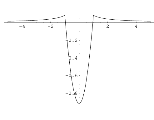
For around a few the potential at the trap entrance at is just barely low enough that an ion will thermal energies of could enter the trap. To clearly settle this case the potential near the transition region would have to be determined more accurately. Also near the electrode the electric field is strong enough that a pseudopotential may no longer be a good approximations. Even if ions created outside the trap can enter the trapping region, clearly they must be cooled more than an ion created in the trap, since an entering ion must lose a few eV of kinetic energy while a local ion must only lose its thermal energy.
In either case, an ion appears in the trap and is rapidly cooled by the cooling lasers. Typically this takes only as long as required for oven to heat up, which is usually less than a minute. This is immediately detected as a large floresence signal in the PMT. At this point the oven and electron beam may be shut off and the laser tuning and alignment and PMT position can be adjusted to maximize the detected floresence.
5.5.2 Counting
The floresence signal indicates a trapped ion, but doesn’t unambiguously indicate the number of trapped ions. More ions should scatter more light, but only if there is sufficient power in the cooling laser to saturate many ions. Typically multiple ions will result in some ions being positions further from the beam axis where the intensity is weaker and often the result is that many ions have a single similarly to a single ions, though usually a few cooled ions do give approximately a simple multiple of the single ion signal, but this is not consistently reliable.
Instead shelving can be used to count the ions. A shelved ion will not absorb cooling light so it will not contribute to the floresence signal until it decays from the state. The decay time is not well defined but has an exponential distribution so that even if all ions are shelved at the same time, they will most likely decay at different times. Then the ions can be counted by applying the shelving lamp until all ions are shelved, which it indicated by the complete disappearance of floresence, then blocking the shelving beam and waiting for the ions to decay. There will be discrete jumps in the signal as each ion decays back to the ground state and begins to again be cooled. Counting the number of jumps needed to restore the full signal gives the number of ions. Similarly the shelving rate can be slowed down enough that individual shelving transitions can be seen by discrete drops in the floresence.
Both methods can require a few attempts to get an accurate count since in some cases two or more ions can react closely enough in time that their individual decays or shelving transitions can’t be resolved, but more importantly for these purposes the presence of more than one ion can be determined quickly, and a single ion easily verified.
5.5.3 Multiple Ions
If more than one ion is initially present, shelving can also be used to reduce the count to just one. Shelved ions absorb no blue light, so they can’t be cooled, neither then could they be heated. Changing the frequency of the blue laser so that it is slightly bluer than resonance heats the ions just as down-tuning cools them. Ions moving away from the laser are more likely to absorb and get an average net extra momentum kick in the same direction as their initial velocity and so their energy increases. This will eventually add enough kinetic energy to an ion that it can escape the trap.
It would do no good to boil out all the ions in this way, but if one is shelved it will not be affected immediately by this re-tuning and will be unaffected while the others are ejected from the trap. Then to reduce the number of ions in the trap, the shelving light can be applied until the floresence signal indicates that one ion has been shelved, or all can be shelved and the decays waited out until only one is left shelved. At this point the cooling laser can be re-tuned to the heating side of resonance. The PMT signal drops as the ions are heated and their orbit increases so that they interact less often with the laser and in weaker parts of the beam. After a few seconds the ions are usually gone from the trap. The laser can be re-tuned to cooling frequencies and the shelved ion deshelved resulting in the desired single ion. This also can take a few tries, with many ions it is hard to be sure that just one is shelved so typically this cleaning out is done in stages, removing a few at a time until only a few remain that can be more easily individually manipulated. Also there is the risk that the shelved ion that is intended to be kept decays while heating the others and is itself heated and lost. In practice these complications are not much of an obstacle and a single trapped ion can be obtained in about a minute after a few of the shelving and heating cycles, only very occasionally losing all the ions.
A safer, but slower and less exciting method of reducing the number of ions is simply to shut off the cooling beams for a while. Collisions between ions will occasionally result in one being knocked out of the trap and after a long enough time letting them many ions fight it out, a single ion remains which is then not further heated by collisions. This process can take anywhere from a few seconds to 10 minutes, but always eventually results in a single ion and seldom fails by losing all the ions.
5.5.4 Isotopes
The particular isotope of the ion can be determined at this point. Different isotopes have slightly difference cooling frequencies, the shift is of order . The OG signal correspond to the most frequent so that by maximizing the count rate with the tuning of the laser, any shift in the transition frequency is easily detected as an offset from the peak of the tuning curve. At least three different isotopes have already been trapped and detected in this way. In addition, when the shifts are known, the cooling lasers can be tuned to preferentially cool a certain target isotope making that more likely to be trapped. This has not been systematically studied, but does seem to qualitatively change the rate at which various isotopes are trapped. This could be enormously useful in practice for doing isotope comparisons.
5.5.5 Ion Lifetime
Immediately after loading, there is a relatively high concentration of Barium in the system even with the oven off. This seems to lead to a reduces lifetime for individual ions in the trap as the are frequently replaced by ions from the background. The trap is too deep for a trapped ion to be knocked out, and the pseudopotential far from the trap repels ions, so a likely exchange mechanism is for a neutral atom that passed through to exchange an electron with the trapped ion and be trapped itself while the originally trapped, and now neutral ion is free to leave.
Usually this exchange would not be detectable expect as some, probably unmeasurable slow, loss of coherence. The exchange can be detected if the new ion is a different isotope as the floresence will change significantly and retuning will yield much different frequencies. This happen regularly a few minutes after loading, especially if the oven happened to be needed to be on for a long period of time while loading. It is never observed more than a few minutes after loading, and rarely when the oven was needed hot for only a few seconds to load, so it is likely that this exchange occurs only when there is much background barium in the system and afterward the ion in the trap after many hours is the same one originally loaded.
Except for this effect there is no limit to the time an ion remains trapped if it is being regularly cooled. When this system is operating ions are lost only due do power failures and tuning errors in the blue laser. Barring these events an ion stays trapped for many days, typically up to a week and on one occasion 6 weeks.
5.6 State Manipulation and Detection
Trapping and loading and cooling finally yield a single ion that is very well localized and relatively motionless. Now a number of precision measurements become possible. The ones that will be particularly relevant in understanding the methods developed for the parity measurement are those that exploit the ability to efficiently detect individual transitions between energy levels of an ion. For a measurement of the PNC lightshift with spin resonance, the initial spin state must set, the spin flip transition driven, and the final state detected. The same coarse sequence involving different energy levels, rather than different spin states in the same level, is followed for various measurements in single ions. The general ideas are best illustrated with a few examples.
5.6.1 Lifetime
The simplest experiment to implement is a measurement of the lifetime. The most conceptually clear way to determine the lifetime is to start an ion in the state, watch for the decay and record the decay time. Averaging the decay times gives the lifetime. With an ion trap this ideal can be realized.
A conventional atomic experiment can effectively do this by preparing a large number of atoms in the initial state and recording the floresence from the emitted photon in the decay as a function of time. This method would be impractical in an ion trap because the detection efficiency of the decay is very low. Though the initial state can be set and detected easily using the shelving lamp and floresence signal, each decay produces only one photon. The solid angle and quantum efficiency of the PMT yield a combined detection efficiency of so only 1 in a thousand decays is detected. An experiment in a vapor, or even a large trapped cloud, compensates for this with a large number of atoms but for a single trapped ion an accurate measurement would instead require excessively long observation times, especially if the background of the detector is considered. An emitted photon would be detected, on average, every . With background from, for example, a dark count of even 1 every few seconds, detecting this occasional extra photon would require that the rate be determined to a part in which then requires detecting some decays, then requiring of observation time to detect a single transition. This is completely unreasonable and detecting a decay in this way is not practical, but with the tools already discussed this transition can be detected reliably with other methods.
The state is the shelved state. In this state the ion will not absorb or scatter the cooling light. Then a transition to this state, driven by the shelving lamp, is detected simply by the disappearance of the blue floresence detected by the PMT and a decay to the ground state is indicated by the reappearance of the PMT signal. The decay time is given by the time between these two large discrete changes in the floresence. Repeating this sequence a number of times quickly yields enough data to reliably determine the average decay time.
This measurement sequence is shown schematically in fig.5.6.

This kind of diagram will be used throughout the remaining discussions of experimental procedures. It provides information about the state of all the light sources used in the experiment at every point in the measurement, a brief description of the purpose of each step, a simple level diagram indicating the transitions being driven or detected and the time required for each step. This measurement sequence yield data like that shown in fig.5.7.

This kind of measurement in an ion trap now avoids complications from effects like Doppler Broadening, collisional quenching and radiation trapping, but this particular method has the subtle disadvantage that the decay is measured while the ion is interacting with the relatively strong cooling lasers. With perfect lasers this shouldn’t have a large effect on the quantity being measured, though non-resonant dipole coupling of the state to other states does slightly reduce its lifetime. In this system the diode laser used for the cleanup transition has some small broadband background that has some non-negligible component at the 614nm deshelving transition so that the time spent in the state is reduced by direct excitations out of it. This could be easily remedied with a simple interference filter, but just as easily it can be avoided with a slightly different measurement sequence that will also avoid the inherent broadening from the off-resonant dipole couplings and be more generally useful for other transitions that can’t be seen directly like this shelving transition.
Instead of continuously monitoring the ion with the cooling beams consider blocking them immediately after the ion has been shelved. The ion now waits to decay in complete darkness, in the absence of any applied interactions. The decay is still not directly detectable, but at any time the ion can be checked to see if it has decayed by applying the cooling beams. If floresence is detected, the ion has decayed during the time waited, if no floresence is seen, the ion is still shelved and so has not decayed. The difference in the floresence in the two cases is some so the ion’s state can be determined with almost 100% certainty in even as little as . With a background of 40-70cps this gives a signal of counts if the ion is shelved and about if it has decayed, these cases are easily distinguished.
Rather than the precise decay time, repeating this sequence many times, for many difference times, fig.5.8, gives the decay probability as a function of time which also yields the lifetime fig.5.9.


5.6.2 Lifetime
A small variation on this latter method of determining the lifetime can also be used for the state. Again the ideal measurement would be to start the ion in this state and measure the decay time, or at least, the decay probability as a function of time. Setting the initial state is easily done with the cooling and cleanup beam. The purpose of the cleanup beam is to prevent the ion prevent the ion from getting stuck in the state by a decay from the state during cooling. So simply shutting off the cleanup beam quickly pumps the ion to the desired state.
At this point the beams can be shut of and the ion allowed to decay back to the ground state. Checking for the decay after some time is no longer immediately possible with the cooling beams as both states are part of the cooling cycle, so the ion would florese whether it had decayed or not, however a single extra step restores this easy determination. The shelving lamp shelves drives the transition so it will shelve the ion only if the ion starts in the ground state. Similarly a shelving transition driven directly by a laser couples only the ground state to the shelved state. In either case an ion in the state will be unaffected, fig.5.10

A decay from the state can then be detected by attempting to shelve the ion by applying the shelving lamp for a brief period of time and then checking to see if the shelving transition was made. If the ion has decayed, it can be shelved and when the cooling beams are applied this state is indicated by the absence of blue floresence. An ion still in the state can not be shelved and will immediately florese when the cooling beams are applied.
The net result is that after this brief shelving step, the ion will likely not florese if it has decayed from the state during the wait time, and likely florese if it has not decayed. The cases are not perfectly correlated from some practical complications, sec.5.6.4, but this sequence does yield a shelving probability that increases with an exponential profile having a time constant of the lifetime of the state. Similarly repeating this sequence for many wait times, fig.5.11, yields the shelving probability as a function of time, fig.5.12, which provide the state lifetime.


5.6.3 Quadrupole Transition
These measurements have so far involved a natural transition, they are just as effective in detecting driven transitions, to measure transition rates or resonance frequencies, such as that spin flip transitions that must be measured to determine the PNC splitting. A simple illustration is with the same state just considered for the quadrupole transition. Here even a conventional atomic experiment could not continuously monitor the state of the transition. The transition probability could be determined as a function of time by turning on the clean-up beam and measuring the amount of blue floresence from ion excited to, or remaining in the state. The amount of blue floresence measures the number of atoms that made the transition. Again for a single ion this would be inefficient since the resulting single photon that signals the transition is very hard to detect, and again this can be remedied using shelving to generate instead an almost arbitrarily large number of photons if the transition was made, and none if it hasn’t.
The ion can be started in either state with the cooling beams as in the lifetime measurement, pumping to the ground state simply requires the complementary case of blocking the blue beam. Light applied to the ion resonant with this transition will result in transitions between the states. A transition can be detected by attempting to shelve from the ground state. Sufficiently monochromatic or intense light will result in a harmonic modulation of the probability of the ion to be in its ground state, yielding an oscillating shelving probability as a function of time. The more easily arranged effectively broadband excitation will give a first order rate equation exponential transition profile. Either can be used to determine the transition rate.
An example of the results of this kind of measurement is shown in fig.5.13. The measurement sequence is similar to fig.5.11 for the lifetime except that the ion is initially pumped to the ground state with the cleanup beam, and the wait is done while applying a broadened laser to the ion to drive the transition effectively incoherently. For short times, or far from resonance, the transition probability is small and the ion remains in the ground state from which it can be shelved so the shelving probability is high. For longer times near resonance transitions are likely and the resulting shelving probability is reduced. The shelving probability then simply decays exponentially with a time constant given by the excitation rate.

5.6.4 Efficiency, Stability, Precision
It is easy to understand how these shelving methods qualitatively yield the desired information about transitions, but there are a few practical considerations that slightly complicate a perfect interpretation of detected floresence after the detection sequence as a transition between the set of states under investigation.
The central feature exploited in these measurements is that an ion in the state can be shelved and an ion in the state can not be. However, this doesn’t imply that an ion in the state will be shelved, or that an ion in the state will not end up shelved. First the shelving rate is finite, so that even when starting in the ground state, the ion may not end up in the shelved state when the shelving lamp is applied simply because it has not yet made any transitions to the state.
Similarly even if it has made a transition to the state the decay may be back to the ground state, where it may try again, or to the state where it is stuck. Then after the shelving lamp is applied for some period of time, this gives a shelving probability, , limited by the shelving rate and the branching ratio of the decay to the decay of about .
The intensity and exposure time of the shelving lamp can be increased so that the shelving transition is saturated, eliminating limits from the rate and leaving the branching ratio limit given , but for this apparatus, the shelving rate is slow enough that waiting long enough to saturate the transition slows down data taking too much so a slightly shorter exposure time is used that typically yields an estimated .
The state has a finite lifetime so that while attempting to shelve from the state that ion can decay from the state and also be shelved, . This depends on the exposure time and lifetime as well as the shelving rate and branching ratio. Typically the shelving step takes only and this effect is negligible since the state is very unlikely to have decayed in this time. Typically, .
Finally, even if the ion has been shelved, this may not be detected by the cooling beams either from counting statistics, or because the ion then decays from the state, or is kicked out by the broadband background in the cleanup laser. This yields a shelved state detection efficiency of .
The net result, with the possibilities that the ion may be in the ground state, and not shelved, , the ion may be in the state, and then still shelved, , and the ion may be shelved but not detected as shelved, , gives a floresence probability, , after this detection sequence of
With the and the state the only possibilities, . Again the residual shelving from the state is usually negligible so that,
The net detection efficiency for a transition is slightly reduced, but the profile is unaffected.
These offsets and modifications depend on experimental conditions and so many be variable and a source of noise or systematic errors in the final measurement. Precision measurements require a careful understanding of this kind of instability and their consequences. This kinds of studies were the central focus of earlier work on this project and the problems and solutions and end results are discussed in [Hendrickson99].
Chapter 6 Spin State Manipulation and Detection
The quantity to be directly measured in this experiment is the PNC induced splitting of the ground state or state magnetic sublevels generated when the quadrupole and parity violating dipole couplings are simultaneously driven with the appropriate phases and beam geometries. One possible route to determining the size of this splitting is to start the ion in a particular sublevel, drive the spin flip transitions and measure the transition probability as a function of interaction time or the frequency of the applied spin flipping fields to get a precession rate or resonance frequency. This will require being able to set and detect the initial and final spin state. The same general procedures are used to manipulate and detect the ion among its different energy levels in more conventional ion experiments. In most cases these spin manipulations and measurements can be made with the same methods modified to make them spin sensitive.
6.1 Pumping
Manipulating spin states by optical pumping is a familiar idea in vapors. The same techniques can be used on a single ion with the only difference being in interpretation of the final result. Rather than pumping resulting in an unequal distribution among particular spin states of atoms in a large population, it will determine relative probabilities for the single ion to be in a given spin state when pumping is completed.
6.1.1 Laser Polarization and Magnetic Fields
Pumping between the and energy levels is easily done with the cooling and cleanup beam. Blocking the laser that drives transitions out the the desired final state uncouples that state. When the ion decays to this state is remains there. Similarly pumping can be done among the spin sublevels simply by uncoupling the desired final state, in this case, by adjusting the polarization of the beams, and the magnetic field defining the quantization axis.

Generally the magnetic field is kept fixed, either parallel to the beam axis or parallel to the linear polarization of the red laser. The applied field is difficult to change quickly, perhaps on time scales of a few tenths of seconds at best without a lot of work, giving a significant limitation to the data collection rate. More importantly, high magnetic field stability is required for the resonance experiments and changing the direction of the applied field dramatically can result in long time scale drifts of the resulting field due to nearby ferromagnetic materials. As a result, in practice, only the laser polarizations are changed to alter the relative spin couplings.
The polarizations of both laser are independently controlled using a voltage controlled variable retardation plate that allows adjustment to vertical and horizontal linear polarization and left or right handed circular polarization.These particular control units are rather slow. Switching polarization states requires times on the order of tenths of seconds, also limiting data collection rates. This is never likely to be the biggest limit, but future improvements may involve an upgrade to the higher speed and additional flexibility, and complications, of a pockel cell.
The red beam also passes through a half wave plate so that the direction of its linear polarization can be continuously adjusted manually. This additional freedom is helpful in aligning the magnetic field as explained later, but is otherwise not necessary. The same ability for the blue laser is not helpful due to the structure of the , transition.
The beams are then combined with a non polarizing 50% beam splitter cube. Afterwards they pass only through a set of focusing optics and to the trap so the final polarization of the beams is unmodified other than by imperfections in the lenses or vacuum windows.
6.1.2 Ground State Pumping
With a magnetic field parallel to the beam axis, and circularly polarized blue light used to drive only transitions, the state is uncoupled, fig.6.2. At the same time the red beam is linearly polarized to include all states.

If the ion starts in the state it will remain there as it can’t be excited by the cooling beams from this state. When the ion starts in the state it will be driven through the and states and at some point decay from the state to the where it will again remain.
With the ion in this uncoupled state, it will no longer scatter blue photons out of the cooling beam to the PMT as it can no longer be excited to the state by the cooling laser. As a result, the count rate drops to the background rate and evidence of this spin pumping is available immediately.
Transition and decay rates are on the order of MHz, so that only a few s is required for a transition to the intended state to be very likely, in a ms it is virtually guaranteed, the fluorescence drops, and the cooling beams can be shut off. Pumping happens very quickly and is practically limited by the switching times of polarization controls and beam blocks well before any limits due to excitation rates, with the end result being the ion in the desired spin state.
6.1.3 Practical Limits to Pumping Efficiencies
In practice, the excitation rate out of this pumped state can not be made to be exactly zero because of impure polarizations or imperfect alignment. This will be considered in full generality shortly, but the immediate consequence is that the ion is occasionally excited out of this pumped state and this results in the occasional blue photon above the background as the ion decays from the state. The count rate then is not exactly the background rate, but is still much reduced, typically to within 20-50 cps of the background, so the PMT count rate is around 100cps including a 30-60cps background compared to 1000cps while not pumping, a reduction in the floresence rate by a factor of 20 or more. This limit is probably largely due to a less than perfectly circularly polarized beam, though it is also possible that some other perturbation would kick the ion out of the pumped state. The latter would require a transition rate of a few tens of kHz, and is one motivation for studying the spin lifetimes discussed later that turn out to exclude this possibility.
The non-optimal configuration also yields a smaller pumping efficiency. The probability to be in the intended destination state during pumping is slightly less than the ideal 100%. As shown later, the rates described above correspond to the ion spending of the time in the state. This is not exceedingly close to ideal, but is, more to the point, far from the 50% uniform probability of an unpolarized ion and is completely sufficient for making spin states detectable and spin transitions visible. The reduced efficiency does eventually result in a decreased experimental efficiency. Improvements might be made with better alignment of the magnetic field and slightly more elaborate control of the polarization to improved the purity of the preferred polarization state and compensate for possible perturbations to it from the few remaining optical elements between the ion and where the polarization is defined. These improvements may eventually be worth considering if they could be made without excess effort as the yield would be small, though they may also be desirable for other purposes.
Finally the residual excitation rate out of the pumped state require the pumping beams to be shut off in a well-defined order. Clearly the red beam must not be blocked first as the ion may be removed from the ground state in the time it takes to then block the blue. The beams can not be blocked simultaneously without considerable effort as the high transition rates result in simultaneous meaning to be within some small fraction of a microsecond. Even if achieved this would still yield a small probability for the ion to end up in the state as the ion does spend some time there during pumping. The best method is then also the easiest, the blue beam must be shut off first followed immediately by the red beam. This also slightly reduces the final pumping efficiency since an ion that is in the state‘ when the blue beam is shut off‘ will be pumped to the ground state by the red but with no preferred spin orientation so it enters either ground state spin level with equal probability. This is a negligible modification since the probability to be in the state to begin with is only a few percent.
6.1.4 D State Pumping
With the same magnetic field parallel to the beam axis and circularly polarized red light with now linearly polarized blue, the and states are uncoupled and the ion is quickly driven to these spin states. With linearly polarized red and a magnetic field now parallel to this polarization axis, only transitions are made on the the state and the ion is driven to the states, fig.6.3.

As for the ground state a pumping signal is immediately visible as reduced fluorescence because the ion lingers in the uncoupled state rather than cycling through the state and decaying. Also, for the same reasons as in the ground state, the order that the pumping beam are shut off is important. In this case the red beam is shut off first, followed closely by the blue.
In these state methods the ion is driven to a set of two selected spin states rather than just one as in the ground state, but the result is still a highly polarized ion in the sense that the probability distribution among the various spin states is far from the uniform, unpolarized case. For the case on linearly polarized red, the probability is evenly distributed between the states. For circular polarization, as seen in the general analysis presented later, the result is a 75% chance to be in the state and 25% to be in the state, and in fact for arbitrary polarizations it turns out the ratio of the probabilities to be in the state to the state is , though this particular solution is unstable and very sensitive to the alignment of the pumping beam, sec.6.1.6.
In principle, these two procedures could be sequenced to yield selection of a single spin state. However, this would require changing the magnetic field between the two cases, which as already mentioned is difficult and undesirable, or using additional laser beams with different propagation directions, also a practical nuisance. In addition, the previously discussed limits of polarization purity and alignment, which prevent any coupling from being made to be exactly zero, make the final state effectively independent of the initial configuration except for particular narrow windows of excitation rates or pumping times because any coupling to a state will eventually result in transitions out of that state. So, in practice, a single step is used and found to be completely sufficient.
6.1.5 General Pumping Analysis
For the idealized cases, pumping is easy to understand and simple to analyze. One beam is used to pump by being set to uncouple a desired set of states, and the other beam is set to couple to all spin states and act a cleanup by keeping the ion in the desired spin multiplet and out of all other levels. In practice, the polarizations can’t be set to exactly the desired states, and the alignments relative to the applied magnetic field can’t be made perfectly precise. So states that are ideally uncoupled, are instead only much more weakly coupled relative to the other states.
In this case, the resulting populations must be determined from the relative rates. The results will be qualitatively quite similar, as the ideal case is simply the limit of a spurious rate returning to zero. The only difference will be in the dependence of the final pumped state on the initial pre-pumping configuration. The precise results require a fully general treatment of the rate equations. As the final configuration does affect detection efficiencies in any future experiment, a more accurate and detailed understanding of the end results of pumping are worthwhile and helpful for planning measurements or evaluating possible new techniques.
The transitions and lasers are broad relative to the excitations rates used, 10’s of MHz compared to a few MHz. So the limit of broadband excitations can be considered and simple rate equations used to describe the evolution of the populations. Lingering coherent effects will be ignored as they would require a considerably more complicated density matrix analysis. This may not be completely appropriate, but the rate equations will certainly capture most of the spirit of the resulting behavior if possibly not all the details.
Take , , to be the probability to be in the sublevel of the corresponding state. and can represent the transition rates of the red and blue laser, and the decay rate from the state to the or states. The dependence of the decay rates is given by the square of the appropriate Clebsch-Gordan coefficients,
With the normalization, , the scalars can be properly interpreted simply as the fractional decay widths of the P state to the S or D manifold and can be written in terms of the total width of the state and a branching fraction . With taken to be the branching fraction to the state, the fractional widths are , .
Excitation rates depend on Clebsch-Gordan coefficients in the same way and, in this case, also the polarization of the lasers.
gives the total excitation rate for a particular transition and depends on the direction of the applied electric field and atomic structure with . The overall rate, can be factored out and the remaining dependence on direction is easiest to understand in terms of the polarization and propagation direction of the applied laser. The fully general case is a bit cumbersome but a general analysis yields the tidy result, [Schacht00],
is more conveniently written as,
giving the rates in terms of three completely independent parameters, , and .
The population of a particular spin state includes a loss from every excitation out of it and a gain for any stimulated or spontaneous decay into it. The equations of motion for all states are,
In all cases the source or destination state is summed over. This allows for a more compact matrix notation. Let be the total loss rate out of a given state due to absorption or stimulated or spontaneous emission,
For the state, the sum of the decay rate over all possible destinations gives the lifetime for a particular spin state. The lifetime will be spin independent so this becomes simply the lifetime of the state.
With these definitions, and moving some indices around for notational tidiness, the matrix form of the rate equations follows easily,
With cooling rates at around a the populations quickly come to their asymptotic values, so only these steady state populations are required for analysis and they are the solutions giving zero time derivatives.
Since the are diagonal, and for the state has no nonzero elements on the diagonal because at least the decay rate is non-zero, it is easy to solve for , as must be invertible,
giving,
This is a simple system of 6 coupled equations which are now best dealt with using explicit algebra or just simply solved numerically. Further manipulations can result in the solution appearing as an eigenvector but this isn’t particularly illuminating and doesn’t make an analytic solution transparent.
An additional simplification is possible if the excitation rates are much slower than the decay rates the can be neglected relative to the . Losses from the state are dominated by decays so becomes spin independent and is given just by times an identity, giving
With . For the work presented here, this limit is generally not valid, the transitions are usually saturated and the excitation rates are of the same order as the decay rates. In either case, only numerical solutions will be presented here so the loss of generality provides no advantage and this form is completely sufficient.
These equations are partly redundant and incomplete. Probability conservation requires that the time derivatives add to zero, so one of the equations is not linearly independent. Also the normalization is not fixed as any scalar multiple of a solution remains a valid solution. Replacing one of the equations with a normalization condition, that all populations add to one, completely defines the problem.
6.1.6 Pumping Signal and Pumped Populations
Final Populations with Ideal Beams
Numerical solutions of the floresence and populations as a function of polarization in figs.6.4,6.5,6.6. Scalar, dipole and quadrupole moments of the resulting populations are also shown, these are helpful in the later analysis and the basis vectors are defined in that discussion. With properly normalized basis vectors, the components are given by .


Polarization Errors in Pumping Beam
These plot show that the final states for arbitrary polarizations and so indicate that they are not particularly sensitive to errors in polarization. However the assume perfect alignment of the beams relative to the magnetic field and it is not immediately clear that small perturbations of this alignment do not yield dramatic differences in the final pumped state. This is easily illustrated for the state.
Consider circular pumping, where ideally only the and states are coupled so that the ion ends up in the and states with relative populations of as discussed previously. Keep the polarization correct by now alter the alignment of the beam. This gives the electric field a small component which will drive the transition, which then couples the state is now coupled as well to the state. This might result in the final state being given by the ion only in the state as it is the only uncoupled state. But with this misalignment the beam is now actually slightly polarized in the plane so in fact transitions are driven and the state is not uncoupled. Clearly now the solution depends on determining the relative rates which requires the correct form of the amplitudes of all the transitions for arbitrary fields.
Fig.6.7 show the populations of the and states with , , as a function of with perfectly aligned and purely linearly polarized blue. As the populations are respectively as previously discussed.

For even very small perturbations in the alignments the resulting residual transition rate quickly cleans out the state and results in the final state being instead composed of full population in only the state. This perturbed solutions actually remains very accurately stable until very large misalignments, . Aligning the pumping beam to a part in would require excessive effort and the most likely beam geometry is somewhere in the stable, misaligned region so for practical applications this perturbed solution should be considered to be the final pumped state.
The other pumping geometries, linear in the state, and circular in the , are not similarly sensitive to this same kinds of misalignment, they remain approximately the same until very large misalignments.
Polarization Errors in Cleanup Beam
The data plotted for ideal alignments as a function of pump beam polarization assumes that the complementary cleanup beam is perfectly set to its ideal polarizations which equally couple all spin states in the other, unpumped, energy levels. For these cases this is always a linear polarization so that that any polarization of the final states is completely determined by the polarization of the pump beam. This ideal is not realized in practice and residual bits circular polarization in the cleanup beam alter the populations. This residual polarization will be small, and it turns out that even it is not the effect on the populations is small, even far from the region of maximum pumping and, of course, at that maximum point there is exactly no change since the desired states are exactly uncoupled.6.8

Floresence and Pumped Spin State Populations
The results are qualitatively intuitive. For polarizations and alignment that significantly reduce the coupling to any state, the floresence decreases as the ion gets stuck in that state and can’t scatter photons as rapidly. This reduction in count rate gives a measure of the time spent in the pumped state by providing an estimate of the ratio of the excitation rate out of the pumped states to the return rate to those same states . At equilibrium the rates times the occupation probabilities for the set of pumped states, , and the set of all other states, , will be equal, so that for , .
Consider an ideally uncoupled state or set of states. An ion that is excited out of this set will be quickly returned to it with some blue photons generated along the way. For pumping in the ground state at least one blue photon is generated in the decay back to the uncoupled state, but more could be emitted by repeated decays to the other spin state. In the state it is possible that no blue photons are generated if the ion immediately decays back to the state, but it is more likely to make a few trips through the ground state first. In either case there is a well defined average number of blue photons generated for every residual excitation out an uncoupled state and the floresence is simply proportional to the sum of the occupation probability times the residual excitation rate for each uncoupled state . For the ground state there is only one ideally uncoupled state, for the state there are two but their populations are simply related at and near the region of optimal pumping for deviations in the appropriate polarization, for linear pumping the populations of the states are equal for arbitrary polarization angles, and for pumping the population is 3 times the population for arbitrary circular polarizations. Then total population and excitation rate of any set of states can be treated as a single state,
When the excitation rate out of the ideally uncoupled states is much slower than the other excitation and decay rates will be very close to 1 as the ion is not frequently excited out of the states. In this limit the floresence is then just proportional to the total residual excitation rate. As as rate increases the probability to be in that state decreases but doesn’t get far from 1 until the residual rate approaches the cleanup and decay rates, . Here the occupation probabilities of all states are similar and so is still of order 1, the examples above show where the populations cross. At this point the floresence is again limited by the decay and cleanup rates, but for most of the way the floresence is simply proportional to the residual excitation rate. This turns out to be an even better approximation in practice because of how the relative populations of the other states increase far from the exact pumping point. fig.6.9 show that the floresence is approximately proportional to the pumped state populations even in for relatively large deviations from the ideal pump polarization.

Taking this to be approximately true for all rates, an estimate of the residual excitation rate at the optimal pumping point, relative to the excitation rate out of the same states when no pumping occurs, which is then about the same as the decay rate, is given simply by the ratio of the floresence at the pumping point to the maximum floresence , . In the region where no pumping occurs , so so that finally the occupation probability is given simply by . For these measurement is typically about to so that as mentioned above.
6.1.7 Pumping and Field Alignment
The pumping signal can be used to align the magnetic field relative to the beam axis and polarizations and optimize polarizations. The applied magnetic field is not precisely known due to imperfections in the construction or alignment of the coils generating the fields. There are also offsets from other magnetic sources which in the case of a local soft ferromagnetic material that can even depend on the applied field, as the directions of the material’s domains are altered by the applied field or ambient temperature, so that the total field can be a complicated or even unknown function of the current supplied to the coils, time and temperature. Nearby probes are little help since unknown sources giving unknown offsets may also include unknown gradients so that knowing the field, however precisely, a few centimeters away from the ion provides no information about the field at the ion. The pumping signal allows the ion to be used as a probe.
For example, pumping occurs for a magnetic field parallel to the polarization axis of a linearly polarized red laser. This provides a means of zeroing the magnetic field along the beam axis. A large field in the general direction of the red laser polarization axis can be applied. If this field is sufficiently large enough to define the direction of the resulting total field some reduction in the floresence due to pumping should be visible. Then, both the angle of polarization can be adjusted, with a half-wave plate, and the magnetic field along the beam axis can be adjusted to minimize the floresence. As previously mentioned, this typically occurs at about 1/10th to 1/20th of the unpumped count rate, though it is ideally zero. The applied field can be reduced a bit at a time and the other parameters adjusted again until the applied field is the desired size. At this point the magnetic field is aligned with the red laser polarization axis, perpendicular to the beam axis. If particular direction perpendicular to the beam axis is desired, vertical for example, the polarization direction can stay fixed and another magnetic field component adjusted instead.
A similar procedure can be used to align the field along the beam axis. With circularly polarized red or blue pumping will occur when the magnetic field is parallel to the beam axis. With an initially large applied field the pumping signal can be used to null the components of the magnetic field perpendicular to the beam axis.
When the directions of the applied fields are well known these procedures are sufficient to determine the magnetic field offset and with that information the field can be reliably set to any desired direction. More often the direction of the applied fields are not precisely known. In this case this alignment by pumping can be done for a variety of directions and field sizes. Eventually there are enough constraints that the size and direction contributions from all the coils can be determined. This processes is a bit easier if the total size of the magnetic field is known, this can be done using the spin resonance techniques discussed later and significantly reduced the number of field configurations that must be tested.
A peculiar feature of the structure of the to transition can also be used isolate the offset. For this transition there are always two linear combinations of states that are not coupled by a red laser with fixed polarization, 4.3.2, they are not necessarily combinations generated from just spatial rotations though they obviously are for the cases of linear and circular polarization. If there is no magnetic field to drive the ion out of these states, the ion gets stuck in these states and pumping occurs just as in the cases already discussed. The floresence drops and this polarization pumping can be used to locate the point where the magnetic field is zero by adjusting the applied field until the PMT count rate is minimized. Some care must be taken to check that this minimum is independent of polarization so that the field is not really zero but just in a direction suitable for pumping with the laser polarizations used.
If the field offset is fixed, some combination of these procedures gives enough information that the resulting field as a function of coil currents can be completely determined. In practice this provided a model of the applied field that was able to predict the size of the resulting field to only about , though for smaller variations of the applied field agreement was better than a few percent. This suggests a significant contribution from some ferro-magnetic materials that would be redirected by the applied field giving an applied field dependent offset. This is an important observation to consider when trying to understand the source of larger than expected spin resonance transition widths. In principle, these contributions could also be identified by a careful study of the resulting field, but no such attempt was made other than to confirm that the contribution was large and nonlinear.
The pumping signal could also be used to tune the polarizations of the lasers. They can be measured independently and are well known outside the chamber, but the final optics, and in particular the window needed to deliver the lasers to ion can alter the polarization after any point where it could be measured before reaching the ion. Any resulting induced circular, or more generally elliptical, polarization could be compensated for by maximizing the pumping signal, this time as a function of laser polarization. This is not completely reliable as there may be continuous flat directions along some combination of polarizations and field directions that always give pumping, [Schacht00], so that some combination of imperfectly polarized beams and a slightly misaligned magnetic field can also give maximal pumping. As a result the pumping signal can not necessarily be used to optimize both the magnetic field and laser polarizations, but some combination of pumping and spin resonance measurements to determine the resulting magnetic field size can be used to determine the magnetic field independent of laser polarizations so that the field can then be set reliably to optimize polarizations.
With enough work, all these imperfection can be uncoupled and all field and polarization parameters determined and optimized. In practice, this sort of precision isn’t really important. The most important result of pumping is that it leaves a spin state that is significantly different than an unpolarized state. This is achieved in any configuration giving a good pumping signal, even including the case of pumping as a result of zero magnetic field. The lack of floresence implies occupation of some uncoupled state and not all the spin states are uncoupled so the ion can’t be unpolarized. Lack of precise knowledge of the magnetic field and laser polarizations then just results in lack of knowledge of the resulting pumped state. The pumped state could be a single single spin state defined along an unknown axis, or some other combination of state not corresponding to a single rotated state, but it is still well defined, if unknown. It does help to have a coarse idea of the parameters to keep track of things, as discussed far more later, maximizing the S/N of the spin detection methods requires that the probed state be the same as the pumped state and coordinating this is easier when fields and polarizations are at least coarsely known. But then coarse knowledge is sufficient and further efforts towards precise knowledge is less important.
6.1.8 Final States
These solutions provide the steady state populations of all of the states during pumping. If the beams could be shut off instantly and simultaneously, or attenuated in unison so that their relative intensities stayed fixed, then these would also be the populations after pumping. General this can’t, or isn’t done in practice. The beams are shut off sequentially so that the ion is sure to at least end up in the desired energy level, if not the ideal spin state. That is, for pumping in the state, the red beam is shut off first, so that if the ion happened to be in the ground state, it is moved to the state. Similarly for pumping in the state. This final pulse from the clean up beam can alter the relative populations of the pumped level.
For polarizations having maximal pumping, cases where the floresence has dropped to zero, this modification will be very small. In these cases the probability to be in the other state is very small so that the final cleaning out of that state will not add much extra population to the pumped state, and so not significantly alter its distribution. For polarizations still yielding significant floresence, there is a significant population in the other state and the redistribution of that population to the pumped state during the final cleanup pulse is an important modification.
It is not immediately obvious that these latter cases are important, but it will be useful in the measurements discussed later to repeat a particular measurement for a variety of initial polarizations. For circularly polarized pumping, there are two fully pumped initial states available. They are generated by using the two oppositely circularly polarized pumping beams. For linear pumping in the state there is only the single fully pumped state. In either case it can be useful to have even more initial states. These will be generated by using non ideal polarizations for the pump beams and then require a careful analysis of the effects of the final cleanup pulse on the spin distribution of the pumped state.
One convenient initial state for reference is an unpolarized state. For the ground state is it clear how this unpolarized state can be generated. With the fully pumped states given by a left and right circularly polarized blue beam, and linearly polarized red, both propagating parallel to the quantization axis, a simple switch to linearly polarized light now couples both ground state spin sublevels equally. With this spin symmetry it is obvious that while pumping the populations of all state in the and levels are spin sign independent, and since no state is completely uncoupled, the populations of all the state in both levels are comparable. A quick numerical result gives,
The final pulse is the linearly polarized red cleanup beam. Again the couplings are spin sign independent, so the leftover population in the state must empty into the state symmetrically to yield,
Trying to generate and unpolarized state in this way is not as clear. Again the result must be spin sign independent, but the relative populations of the states to the states is not immediately obvious. The correct final state can be determined with the rate equations for this system,
For simplicity consider any stimulated decay rate to be negligible compared to radiative decays so that, in particular, . With , implying , this gives,
The final state populations during the last bit of application of the cleanup beam are given by the integration,
This can be written formally in term of the solutions of the ground state populations using the eigenvalues of . This gives solutions of the form.
Which can easily be integrated.
Giving, formally, the final populations,
These eigenvalues and eigenvectors can also easily be determined numerically. For circular pumping in the state, using circularly polarized red, linearly polarized blue, and magnetic field parallel to beam axis, linearly polarized red light and the final blue cleanup pulse yields the state,
This is not precisely unpolarized, the populations are certainly significantly different from the pumped state, which will turn out to be all that is really important for detecting transitions. For linearly polarized pumping in the state , using linearly polarized red and blue, and magnetic field perpendicular to the beams, a circularly polarized red pump beam and final blue cleanup pulse,
Solutions for other polarizations for the state are given from the same calculations. The same procedure can be used to determine final ground state spin distributions for arbitrary pump polarizations, though the analysis is a bit more complicated as four eigenvectors and eigenvalues are the required. These few solutions show that a significantly different initial spin state is available with a simple change of pump beam polarization and approximately unpolarized states are possible.
6.2 Spin State Detection
While setting the initial spin state of a single ion is relatively straightforward, determining an unknown final state is more subtle. In a vapor this spin state can be determined with a probe laser in a variety of ways, but none can be directly applied to the case of a single ion.
6.2.1 Vapor Methods and Single Ions
With a magnetic field parallel to the propagation direction, resonant probe light will couple transitions. As an illustration, consider spin detection in the ground state. The issues for the state are almost identical, only details of the structure of the transition are different.
Absorption
On a transition, atoms in the state will absorb photons of only one helicity, while atoms in the state will absorb photons of the opposite helicity. This picture would be slightly more complicated in more general cases such as a transition where both spin states can absorb photons of either chirality, but in this case the relative rates are different and you simply get atoms in one particular spin state preferentially, rather than exclusively, absorbing photons of a particular chirality.
In either case the net effect is qualitatively the same, with an excess of atoms in one spin state, more photons of one helicity will be absorbed and scattered out of the beam than of the opposite helicity. With incoming probe light linearly polarized, the net effect would be an induced elliptical polarization of the probe after interacting with the atoms by an amount, and direction, dependent on the relative spin states of the atoms.
A direct application of this method to a single ion could involve using the blue cooling laser as a probe and looking for changes in its final state as a result of the spin state of the ion. In this case the reduction of the system from a macroscopic collection to a single ion is fatal. The resonant interaction of the light with the ion destroys the spin state of the ion. After absorbing a photon and being excited to the state, the ion can decay to either spin sublevel in the ground state. The branching fraction for decay to each sublevel is different, the ratio is given simply by Clebsch-Gordan coefficients as 2:1, so the final state of the ion, and probability for absorption of a second photon is slightly different for different initial spin states. For this particular system, there is also the possibility of a round trip through the state before returning to the state further diluting the final dependence on the initial spin state. As a result, after absorbing even just a few photons, the information about the initial spin state of the ion is lost and the ion will absorb photons of either helicity without preference.
In this way, the final state of the probe beam would be altered by the loss of at most a few more photons of on helicity than another and the resulting change in the probe’s polarization state would be undetectable.
Optical Rotation
A more common method in vapors is to use off resonant light as a probe. Here absorption is negligible and instead the net effect is easiest to understand as a difference in the index of refraction for left or right circularly polarized light propagating through the vapor by an amount dependent on the relative spin states of the atoms. This will give a different relative phase of the two components, and appear as a rotation of the plane of polarization of the probe after it exits the vapor.
The amount of rotation depends linearly on the number of atoms, so again this method fails for the single ion because of number. A rotation of even a few full revolutions in a vapor with or more atoms corresponds to an undetectably small rotation for a single particle though perhaps it is possible that variations of this method could be made to work by, for example, putting the ion and the probe light in a cavity so that the same light could interact with the ion many times before being detected.
Fluorescence
Finally, consider again a resonant probe beam. Now, instead of looking at the final state of the beam, which is basically the light that didn’t interact, look instead at the scattered probe light. Using a circularly polarized beam to excite, for example, transitions, only atoms in the can be excited to the state, and so only those will scatter the probe light. Atoms in the state will make no contribution to the fluorescence. The population among spin states then appears as a change in the number of detected photons from some baseline corresponding to an unpolarized state. An increase in the number of atoms in the state is an increase in the number of atoms able to absorb the incoming probe light and so an increase in fluorescence.
A decay from the state can be to either ground state sublevel. If the decay is to the state, another photon can be scattered by the same process. Eventually the final state will be and fluorescence must stop, so each particle can generate at most a few photons. For a single ion in a trap these few photons are the entire signal but with the previously mentioned detection efficiency on the order of a part in a thousand these photons will most often not be seen and so about a thousand trials are necessary to begin to be able to distinguish spin states. Detection is possible, but sensitivity is far too low to be of any practical use, 5.6.
The situation can be slightly modified when considering other transitions for spin detection such as using the state rather than the . With probe light again set to excite transitions, an ion initially in the state will be excited to the state. From there, if the ion decays back to the ground state it can only go back to the sublevel, as it can change by at most 1. So in this case the ions starting in the level can scatter photons as long as the probe beam is on, but now, ions starting in the level can also. From that level, ions are excited to the state where they can decay back to either ground state, both of which can again be excited and in the end the ion will end up in the same loop as when starting from the state. The excitation rate is slower out of the state by half, so one spin state may generate a few more photons than the other, but low detection efficiency also results in this method having low sensitivity and even this difference is slightly eroded by possible decay to the state from the state which results in further loss of information about the initial spin state.
6.2.2 Shelving
In each case direct application of vapor methods to spin state detection in a single ion fails because of low sensitivity and detection efficiency and so something fundamentally different must be considered. At the higher level, and lower resolution, of distinguishing the state of the ion between different energy levels, similar difficulties exist and these have been solved with great success using now well established shelving methods, 5.6. Modification of these methods to make them spin sensitive finally becomes a practical means of spin state detection.
6.2.3 Shelving Laser
To generalize these kind of techniques to detecting spin states, the simplest idea to consider, and most straightforward to analyze, is a modification of shelving by direct coupling to the shelved state with a 1.76m laser. As with pumping, the laser polarization and magnetic field direction can be chosen to couple only particular spin states to make transition rates spin dependent.
Consider again transitions. The structure of the transition doesn’t leave either state completely uncoupled, but the is faster then the transition by the ratio
This can be exploited in two ways,depending on the nature of the light used to drive the transition.
The most conservative assumption is that the laser linewidth is sufficiently broad, and the transition rate sufficiently slow, that the laser is effectively broadband and the transition is being driven incoherently. In this case probabilities evolve as simple first order rate equations. Neglect any spurious couplings to unintended states, though they would be important at long times and modify the steady state probabilities by the ratio of g-factors. This then gives simple exponential excitation profiles with different time constants for the different spin states, fig.6.10.

The ground state spin can then be determined by measuring the shelving probability since for a fixed time, the shelving probability is a function of the initial spin state.
Maximizing detection efficiency requires maximizing this difference. For short times, neither spin state has a large shelving probability so the difference is small. At long times both state have reached the same steady state value and the difference is zero. The spin states can only be distinguished in a particular range of times so the shelving time must be well chosen. With the steady state shelving probability and the rates given by and , the difference is . This is maximized at the time , and at the difference depends only on the ratio of the rates ,
Both and give the same result for , except for the sign of . Generally the rates aren’t known well enough to be able to use the optimal exposure time. At time the difference becomes .
This case gives , , at . The difference is small, though certainly detectable. However it can be greatly improved if the transitions can be driven coherently. With a narrow laser linewidth and sufficiently high transition rate, the width of the laser can be neglected and assumed to be monochromatic. For this case the probability just oscillates between an and a state with a frequency given by the square of the matrix element. Since the couplings from the two spin states are different, the oscillation frequencies are different and again the states can be distinguished by a difference in the shelving probability as a function of time. With a ratio of rates of two, or any integer, the difference can be 100%. By driving the transition until the slower transition, here the , has completed a half cycle, the faster transition has completed a whole cycle. A pulse for one is a pulse for the other and the shelving probability is the ideal 100% for one spin state and 0% for the other, fig.6.11.

This can work from the state as well, though the energies are very different. The to is far in the infrared at . The additional structure of the state makes things a little more complicated. For transitions, the ratio of frequencies is,
This gives a 100% discriminant between and at , with the period for the slower transition. For transitions there are four rates,
Spin detection using the shelving transition directly in this way yields the ideal 100% detection efficiency but with the considerable technical complications of a very well stabilized, high power laser and carefully timed pulses. Driving the transition coherently with a laser stabilized to even 100kHz requires a transition rate of about a MHz. This rate electric field strengths of using, for example, a mW laser focussed to a spot. This may be pursued if the S/N of other methods proves insufficient.
6.2.4 Shelving Lamp
Shelving through the state can also be modified to be sensitive to spin, again by choosing polarizations and magnetic fields that drive only transitions. Here also both ground state spin levels are coupled and a spin discriminant requires exploiting different relative rates. In this case, coherent transitions would not be useful. On resonance, with the transition rate very much faster than the decay rate out of the state, the ion can simply be considered to be in either relevant state with 50% probability, from which it could decay to the shelved state. But the decay rates are spin independent so the ground state sublevels cannot be distinguished.
As the transition rate slows, the populations evolve less coherently and the spin states can be distinguished. The largest disparity is when the transition is completely decoherent. This situation is also the easiest to analyze and the most appropriate physically since in the current system the shelving transitions are being driven broadband by a discharge lamp.
Rate Equations
The previous analysis used for pumping can be used directly. The structure of the system is a bit different in that the state can decay to either of two states, but this doesn’t change the form of the equations. With in this case, and also assuming that , the rate equations from sec.6.1.5 become,
With the population evolve quickly to a quasi-independent steady-state value and we can take . include only decays so is spin independent, . Take as it is now the only excitation rate in the problem and drop the state terms, they will be given by normalization. This gives and . is the matrix describing the relative rates of decays to particular spin states and is just the usual total decay rate, so the overall rate drops out. With with the branching ratio to the state compared to the state and the appropriate matrix of squares of Clebsch-Gordan coefficients the rate equation for the ground state becomes
is well defined but not well known so left as a variable which also allows for the easy application of this solution to other systems.
This leaves a single uncoupled equation. The populations can be derived from this solution but the spin details aren’t necessary for this analysis. The quantity of interest is the shelving probability, which will be the final probability to be in the state. Summing over spin state for either state,
Each state evolves with the same structure but a rate given by its branching ratio. Then at any time, the relative population among the states, which is just that missing from the states, is given by these ratios. In this case this is 90% to the . So the evolution of populations among any of the states is given simply by the solution for the state.
Solution
Clearly the ground state spin can not be determined with a linearly polarized probe beam, so consider pure circular polarization selecting transitions. The desired solutions are for the total population of the ground state as a function of time when starting from a particular spin state. For this 2 dimensional first-order linear system the general solution is a sum of exponentials with 2 time constants.
For this problem one of these solutions is trivial. As previously discussed for pumping, and ion beginning in the state will be excited to the state, at the excitation rate , from which it can decay to the states, and be shelved with 90% probability, or back to the ground state with probability and so a rate . The decay to the ground state can only be back to the level for this dipole decay to the ion stays in this cycle until it reaches a state. So the initial state decays with time constant and the population in the ground state decays with the simple single exponential.
The solution for an initial state of spin down is less obvious, though straight-forward. The excitation rate from the state is a factor of 3 slower, as given by a simple ratio of Clebsch-Gordan coefficients,
In this case the decay to the ground state can be to either spin sublevel and a decay to the level is preferred
So the branching fraction to the state is 2/3. The initial spin information is quickly lost as the populations soon evolve identically and both decay as if starting from the state.
These processes completely describe the evolution of the system. The repopulation rate of the state is , and of the state is . This gives all the terms in the rate equation coupling matrix.
The scalar overall excitation rate factors out, and with , can be scaled away.
The detailed behavior for this particular problem is easily obtained with a bit a algebra, but a more general analysis is not much harder and will be useful for other processes to be considered later. An eigenvalue/eigenvector solution is the most transparent. There will be two eigenvectors, call them , and two eigenvalues . The eigenvectors evolve simply as . The two initial spin states will ideally be pure spin up and pure spin down, but to allow an easier analysis of systematic errors involving impure polarization state, misalignment of axis and incomplete pumping, and for later work with lifetimes and transitions, it helps to consider the more general case an initial states.
The probabilities can be fully parameterized by a single variable, a convenient form is , or which is already expanded in terms of the usual spherical multipole moments. To make things even more efficient, these basis vectors can be derived from the identity matrix and pauli matrices by operating them on a column vector of s, with , as . For diagonal matrices, such as the and used here, this simply gives a column vector of the diagonal elements of the matrix. The matrix dimensions will be clear from context and so the can also be dropped. Then the state is just written as
From this it is clearer that is just the spin polarization, .
The state can be written in terms of the eigenvectors as,
This immediately gives the time evolution by . The absolute probability is not as important as its dependence on the initial spin polarization, so it is convenient to just compare this result to some reference state with some different . A natural comparison to the unpolarized state with . The independent pieces just cancel to give,
The total population in the state is just the sum of the populations in each spin state. Summing the components of the column vectors gives,
and the difference is just proportional to the difference of the initial spin polarizations.
For this problem the rates are given by . For the eigenvectors, as argued above and it turns out . This yields,
With , this yields at . This ideal is reduced by the previously discussed branching ratio to the state of about 10%, which gives a maximum shelving probability of 90%, and the shelved state detection efficiency, the probability that a shelved state is detected as shelved which is less than 1 because the finite lifetime of the state might allow the ion to decay while checking for shelving. The detection efficiency depends primarily on the time taken to check for shelving, which in turn is limited by the PMT fluorescence signal and background. Observations times are generally , and the state lifetime is about 10s, when the cooling beams are on, giving detection efficiencies of . These reduce the theoretical maximum discriminant to at least 80% of its ideal value, . Ideally the initial state can be polarized fully in either of two opposite directions for , and the comparison of shelving probabilities between these two cases is twice the just given.
Experiment
The resulting difference in shelving probability is smaller than for the techniques discussed later, but it should be detectable and was the first to be tried since it is the easiest to implement. A simple two step experiment was used to study the techniques and determine if it would yield a usable spin discriminant. After cooling the ion the spin state is set using the pumping methods discussed in Sec.6.1.2 to one of the spin states. Immediately after these pumping beams are shut off, the circularly polarized shelving lamp is applied for fixed times of about a second, the shelving lamp is blocked and the ion’s state is determined by again applying the cooling beams with polarization set for cooling and detection. No fluorescence indicates a shelved ion. The result is recording and the entire sequence is repeated with a second, different, initial spin state. Both cases are repeated until the statistical uncertainty is small enough that a discriminant can be detected, this is typically a few hundred trials. A detailed diagram of the measurement sequence and timing is shown in fig.6.12.

The sensitivity of this detection procedure to the ions initial spin state should appear as a difference in shelving probability between the two cases.
The details of this particular implementation of this method require some modifications to the previous analysis. The shelving lamp was circularly polarized with a linear polarizer and a wavelength specific quarter-wave plate. Relative angle alignment was coarse but good providing at least 90% circular polarization. More importantly, physical constraints required that the shelving light propagate at a 45 degree angle relative to the quantization axis define by the pumping beams. This could be accounted for by modifying the probe polarization in the previous analysis, but it is easiest to temporarily just rotate the states and use the previous generalized results for an arbitrary initial state. After rotation in a plane containing the z axis a spin up state becomes . For 45 degrees, this gives a probability distribution of or giving . Also limitations in the polarization control of the blue pumping beam allowed for circular polarization of only one handedness, so the comparison was made between this resulting pumped state and an unpolarized state generated using linearly polarized blue light giving rather than completely opposite polarizations and the discriminant yields only one . Finally, since the shelving rate is not precisely known it is difficult to pick the optimal shelving time. An error in the rate of a factor of two gives a further reduction in the discriminant by about a factor of two or more. This makes the signal marginally detectable.
The actual experiment yielded a discriminant of only about 1.5%, Table 6.1. It was reproducible and reversible but it is just at the edge of statistical limits for these ~thousand trials of so it is far from a reliable detection. Improvement could be made. The loss due to the branching ratio could be reduced by using the usual red cleanup beam to return the ion to the ground state but this considerably complicates the analysis and most of the spin information is lost in the many decays and excitations back into the probe cycle, and anyway this problem is far from the biggest limit on spin detection efficiency. More important is to improve pump polarization, align the shelving lamp with the pump beam axis, and accurately determine the ideal shelving time. These improvements could be made with some effort, but such work was put off in favor of pursuing method with inherently better signals which, in addition, eliminate the sensitive dependence of the discriminant to the probe rate.
6.2.5 Pumping Beams as a Probe
Ground State Spin Detection
The fundamental problem with ground state spin detection through an intermediate state is the high branching ratio for decay back to the ground state which leads to a loss of the initial spin information. This penalty is particularly high when using the state since the preferred decay from the state is to the state compared to the by a factor of 2:1, so that evolution profile of an ion beginning in the state quickly merges with that of an ion beginning in the state. This situation is reversed in the case of excitations to the state. Here the preferred decay from the state is to the state, again by a factor of 2:1. Then an ion starting in the state, excited to the state by circularly polarized light and not decaying to the state will most likely return to the spin state from which it started where it can make another attempt for the state. This partial preservation of the initial spin information in the decay delays the dilution of that initial spin information and allows a much larger discriminant.
In this case, the state ideally is completely uncoupled and the end result is the ion in the or state depending on its initial spin information. To complete the process, a conventional, spin independent, shelving step is added. Then an ion starting in the state remains there during the spin sensitive probe step and is shelved during the shelving step, while an ion beginning in the state is possibly moved to the state from which it won’t be shelved.
The same beams and polarizations used to pump the ion can be used for this spin sensitive probe, making implementation rather easy, though they must be highly attenuated or quickly switched as discussed later. The method is a bit more roundabout, requiring an extra shelving step, but the ideal discriminant is twice as large as that for using the state. And since the state is uncoupled, it turns out that it is easier to realize this ideal making the state a far more tractable means of spin detection.
The detailed analysis is the same as for the state. The time evolution is determined by,
Again there is one trivial eigenstate, with , and it turns out with, as is clear by inspection, , so . Since one of the rates is zero, the maximum discriminant is simply at and the actual rates aren’t important. Substituting this we have,
which reduces, for this case, to,
Note that this has sensible limits for and . For and the ideal this gives . For a comparison between oppositely polarized initial states, , this is a difference of in the shelving probability. This ideal value is also slightly reduced by shelving and detection efficiency as before by a factor of about 0.81 to .
The difference is independent of the rates, it is no longer important to accurately know the probe rates, provided they are applied for a long enough time. So a reduction of this ideal rate because of an incorrectly chosen exposure time is no longer a factor. As a practical matter, the rates are still important to consider. Since the probe beam will not be perfectly polarized the spin up state will not be completely uncoupled. If the probe beam is applied for too long, both spin states will be emptied. Therefore exposure times should be chosen to be not longer than a few to fully empty the spin down state and minimize loss from the spin up state. For this work the pumping beams are also used as probes, as proposed earlier. The pumping and cooling rates are MHz, so at full power, microsecond switching times would be necessary. This alone is possible with the right hardware, but it is also necessary that when the beams are ’off’ the rates are really zero on times scales of a few minutes. This requires attenuation ratios of about , current devices, like pockel cells, provide around without too much works. Alternately, mechanical beam blocks can easily provide this kind of extinction, but switching times are limited to a few ms. For this work, the pump beams were attenuated so that their excitation rates were are around a few per second for use as a probe, and a beam blocks on stepper motor were switched at times on the order of tenths of a second to provide the ideal exposure.
This method also has the advantage that the probe polarization is the same as the pump polarization. Recall that in attempting to implement the case of the circularly polarized shelving lamp physical constraints prevented being able to align the axis of the shelving lamp with the pumping lasers and this contributed a loss in the resulting spin discriminant of a factor of 2. In general, maximizing the spin discriminant requires probing the same state that was pumped which then requires that pump and probe light have the same polarizations. This requirement is automatically satisfied for this method since pump and probe light are the same. This is partly complicated by the fact that two lasers are used for pumping while one is used for probing, and the pumped state is exactly determined by both pump lasers. As discussed in the pumping, sec.6.1, ideally one laser is linearly polarized to equally couple all of its states and act as a cleanup while the other is used as the pump to select a particular state to empty. If the cleanup laser has some residual circular polarization the resulting pumped state is somewhat altered, though the effect is small, and with a perfectly polarized pump the shift is zero as the desired state is exactly uncoupled. As a result the the probed state is almost exactly the pumped state and the spin discriminant is maximized with no additional effort.
This method works just as well for spin detection in the state and it turns out to have an even larger discriminant. So this technique was tried first in the state to make study and optimization easier and work on the ground state put off.
D State Spin Detection
The same branching ratio that makes spin detection in the ground state difficult using a state, make it very easy to detect the ion’s spin in a state. A ion excited with a probe from the state to the , would most likely decay to the ground state rather than back to the state by a factor of 2.85. With this spin detection is done in one step. This advantage is partially eroded by the structure of the decay back to the state, as with the the probe but this is less important and the resulting discriminant is much higher than for the state.
For the state there are two probe possibilities that are worth considering. Like for the ground, light can be used. In this case, for for example, an ion in the or states will be excited and possibly moved to the ground state, from which it can then be shelved, and an ion starting in the or states will remain in the state, and not be shelved. Here there is also the possibility of using a probe. This will result in the states being emptied, and the states being untouched.
Again the detailed behavior is given by the same rate equations with the only difference being the dimension of the problem. Before looking at any particular case, consider the general structure of the problem. For this 4 dimensional system there will be 4 eigenvalues, but since the excitation is to a spin intermediate state, two of these eigenvalues will be zero. This is obvious from the special polarization cases just discussed, but it is generally true as well. The evolution of the ground state will then be given by a constant plus two decaying terms. For long times only the constant terms will contribute. So to get the probability of remaining in the state, only the coefficients of the eigenvectors with zero eigenvalue in the expansion of the initial state are required.
The simplest case is the probe,
In addition to the trivial eigenvectors, written here for convenience as,
are
An ion starting in the fully linearly pumped state, will remain in the state after probing. This should be compared to a completely unpolarized state since the exact complement, , can’t be generated directly. The state will decay, leaving , giving the total state population . Relative to the pumped state, this gives,
With , . This would turn out to be if compared to the complement to the pumped state.
For circularly polarized light with ,
The algebra begins to get a bit cumbersome, but the strategy is the same. In the end, for the fully circularly pumped state, which is in practice, fig.6.1.6 ,
The complement state can be generated with an oppositely circularly polarized pump beam giving
and a maximum possible discriminant,
This discriminant is larger than for the linearly polarized probe completely because oppositely polarized states can be compared. Just for reference, an unpolarized state in the basis would yield
Again, both are slightly reduced by the shelving efficiency and shelved state detection efficiency.
As with the ground state, a solution for a general initial state would be convenient for studying transitions and systematic errors. The is not quite as straight forward as three variables are required to parameterize the populations. An expansion in the spherical tensor basis is still most convenient,for this dimension 4 problem the basis vectors are
The normalizations are not conventional but they aren’t important and these are the tidiest with a minimum of fractions and roots in the end. Then the state is written as,
To get the final occupation probability for this state, again write the basis vectors in terms of the eigenvector, take the long time limit so any eigenvectors with nonzero eigenvalue will give zero at long times, and sum over spin states. Note that this last step also eliminates contributions from eigenvalues whose components sum to zero, such as from case of linear polarization as its components were chosen to sum to zero, and in the end only the component of contributes to the final probability.
For the case of linear polarization,
For long times, gives zero, and summing over spin states, gives 2 and gives 0, so
Similarly , and . Comparing to the unpolarized case, this yields,
Giving the tidy result that the final probability depends only on the amplitude of this quadrupole moment. This is consistent with the previously considered case , or , so .
As before the result for circular polarization requires less tidy algebra. The result becomes,
For pumped state, which is in practice, , , , ,
as before. For the complement to the pumped state , , , , yielding,
Experiment
This method was tested in the same way as for chiral shelving for both polarization schemes. A typical measurement sequence is shown in fig.6.13, for a circularly pumped initial state and circular probe. For other measurements, the spin pump and probe polarizations are altered, as well as the cleanup beam polarization if appropriate. A probe beam was supplied simply by mechanically blocking the brightest part of the red cleanup beam and letting the weaker diffuse light pass through to the ion.

First a preparatory step is required to the the probe rate properly. The ion is set to the state with the blue cooling beam, the blue beam is blocked and the attenuated red beam with polarization set to couple to all the states is applied for a fixed time, at first a few seconds, lately a few tenths of seconds. The red beam is blocked and a shelving attempt is made. The red attenuator is adjusted so that the shelving probability shelving probability after the probe approaches the maximum shelving probability. This guarantees that the rate and interaction time is long enough to empty a spin state to the ground state, but not so long that all are emptied because of residual couplings to those state from an imperfectly polarized probe beam or beam axis or magnetic field alignment.
When the probe rate is properly set the spin detection test can be made. For either spin probe scheme the ion was prepared by pumping with one of two polarizations. For the linearly polarized spin probe, there is a spin polarizing pump polarization, linear, parallel to an applied magnetic field and and reference pump polarization which was chosen to be circular, which would yield an unpolarized state for the same magnetic field. For the circularly polarized spin probe, the polarizing and reference pump polarization were simply left and right circular polarization, in this case the reference polarization also polarizes the spin state. Immediately after the state is prepared it is probed with the red beam alone set to the spin polarizing pump polarization. A shelving attempt is then made, and the shelving probability as a function of pump polarization is determined. The shelving polarization should be lower when trying to shelve and probe the pumped states.
A typical result is shown in fig.6.14for a linearly polarized probe.

The shelving probability is plotted as a function of trial number for two cases. The pumped line gives the shelving probability after probing a spin polarized state. The shelving probability is low for this case because the ion tends to stay in the pumped states, the
states, so during the probe, which couples only the states to the state, it remains in the state and will not be shelved. The unpumped line shows a higher shelving probability since the ion more often begins in the states from which the probe beam can move it to the ground state and then be shelved. There is a difference in shelving probability of about . This dependence on the initial spin state is apparent even after only a few trials and the initial state can be determined reliably after about a hundred trials.
An example of results from a circularly polarized spin probe is shown in fig. 6.15.

In this case the ion is pumped to the states the states and the probe only empties one of these sets of states. When the probe and pump are the same polarization, the probe is probing an emptied state and the shelving probability is low. For opposite polarizations the ion starts in the probed states and the shelving probability is high. Here the difference is about , larger than for the linear polarized probe, as expected, and again, easily and quickly detected.
For both cases the discriminant is only about 1/4 of its ideal value. As for the ground state, this is most likely due to imperfectly polarized beams and misaligned fields. This reduces the difference in the initial spin states of the ion, reducing the maximum possible discriminant, and also makes the discriminant probe rate sensitive, which then requires a more careful determination of the optimal probe time. No optimizations were made, other than an occasional adjustment of the probe rate using the attenuator, as the signal resolution was completely sufficient for the studies discussed presently, but when maximizing S/N becomes important later substantial improvement should easily be available here. However, as a practical consequence of this neglect, the particular values for the shelving probability can’t easily be predicted, as they are dependent on the details of the implementation, so they must be remeasured when needed in any particular experiment. But this is easily done as just described and no great burden.
The reduced discriminant could also be due to a shortened spin lifetime, which would erode the difference in spin states while probing, and as a result also reduce the discriminant. This possibility is important to consider as it affect the sensitivity of a parity measurement as well. Such limits can now be studied in detail with these spin setting and detection techniques.
6.3 Spin Lifetimes
These probe methods provide a spin dependent shelving probability, and with it, its inverse, a means of determining the initial spin state from the shelving probability. With only this tool, spin lifetimes can be studied. The parity experiment requires measuring a shift of about a half Hertz. Generally, this requires measurement trials of a few seconds or tens of seconds, either to watch it precess or to drive the transition slowly so that it has a sufficiently narrow linewidth. This is a relatively long time for atoms, where many processes happen at megahertz rates, and it is reasonable to worry that there are processes that could completely scramble the spin well within that time scale such as off axis fluctuating magnetic fields, or stray DC electric fields, or even the trapping fields themselves. The details of the ion’s environment are not completely known at the levels which this experiment’s sensitivity now requires. The spin needs to stay put on its own long enough that when it is observed to change it is only because of an applied interaction.
For the parity experiment there is already a process known to shorten the spin lifetime. The parity laser will couple the ground state to the state. This state has a finite lifetime of around 50. A given ground state spin sublevel can make a transition to the other spin state through an excitation and decay through the state. In terms of the new energy eigenstates this appears as a finite spin lifetime, in this case, for a transition driven to full saturation the resulting spin lifetime will be twice the state lifetime. At that level this is not a problem, though it is also the case that the state lifetime, and do the resulting spin lifetime, is shortened by off-resonant couplings of the state to other and states driven by the intense electric field of the parity laser. In any case this is all well known, and the concern at present is to processes driven by unknown environmental perturbations.
A spin lifetime longer than a few tenths of milliseconds is already implied by existence of pumping signal in the fluorescence. The reduced rate that appears during pumping is probably determined by pump beam polarization or alignment errors, but it could, in principle, be limited by a short spin life time for the pumped state. If the spin lifetimes were very short, microseconds, the ion wouldn’t stay in the uncoupled spin states long enough to significantly reduce its time in the state and so reduce the blue fluorescence produced by decay to the ground state. Instead here the count rate drops by a factor of about 100, from megahertz to tens of kilohertz, implying that the the ion spends at least a few tenths of microseconds in the pumped state.
The appearance of a spin discriminant provides an indication of an even longer spin lifetime. The polarized probe beam is applied for times of up to a second. If spin lifetimes were much shorter than this the spin would be unpolarized before probing was complete and any any dependence on the initial spin state would disappear since the initial spin state disappears before probing is complete. The spin discriminant is already less than expected, this could be the result of an already partially decayed spin state. And even if not, this alone is not enough to probe lifetimes of many tens of seconds which is the real goal.
These longer times are easily studied with a simple modification of the experiment used to generate the spin discriminant. After the pump step, instead of immediately applying the probe beam, wait a fixed time with no light on the ion, then apply the probe beam and attempt to shelve as usual. For a finite spin lifetime, any initial spin state will decay to a unpolarized state and eventually the shelving probability will become independent of the initial spin polarization.
6.3.1 Ground State Spin Lifetime
Consider for now just incoherent perturbations that can be understood as a relaxation, rather than coherent effects that generate energy shifts. The former reduce signal to noise and sensitivity while the latter are included when analyzing systematic errors. Relaxations in the ground state are the easiest to account for as they have the simplest structure. The fully general case is a dipole coupling between the two spin states. The result is simple an exponential decay of the polarization, but to prepare for the more complicated case consider a more formal development. The time evolution is given again by a first order rate equation as with off diagonal elements given by Clebsch-Gordan coefficients and the diagonal elements set to conserve probability by setting them to make rows and columns sum to zero, or , as this gives . For this spin problem, is simply,
with some rate.
Again eigenvectors are the most direct path to the solution, here they are , , or simply and , if as before, these are understood as vectors derived from the usual matrices operating on a column vector of all ones giving just the diagonal of the original vector. The eigenvalues are and . The vector with eigenvalue will always appear in the general case. It must to conserve probability, and it is clear mechanically. If all the rows sum to zero than any row operating on a column vector of s will give zero. As a result, the elements of all the other eigenvalues must sum to zero since the accounts for all the of occupation probability.
The state, as written before, already appears in this basis as . The component decays and the full time evolution is simply
The spin discriminant then also decays with the same time constant,
Experimental studies of spin lifetime in the ground state were limited because of the low discriminant achieved with the chiral shelving spin probe method. Data was taken for two wait times, s and s. The results are shown in table.6.1. Each case is derived from about 1000 trials giving a statistical uncertainty of 0.012. The shelving probabilities for a linear or circularly polarized pump beam differ by about 1. The shelving probabilities as a function of initial spin state are basically independent of time implying spin lifetimes of at least 5 seconds and most likely 10 or more.
| 0.5s | 5s | |
|---|---|---|
| 0.189 | 0.186 | |
| 0.174 | 0.176 |
6.3.2 D State Spin Lifetime
A more extensive study of spin lifetimes was done in the state because the much larger spin discriminant obtained made work easier. This four state system is considerably more complicated, making analysis a bit more involved, but giving a richer structure that can provide more information about the ion’s environment. As with the ground state, a perpendicular fluctuating magnetic field could be considered with the same dipole couplings. Another source of decoherance could be fluctuating static electric fields, or even the applied high frequency trapping fields. The effects in the ground state would be indistinguishable from a magnetic field as dipole couplings are the only interactions that can fit into a spin 1/2 system. In this state quadrupole interactions are allowed, either from direct couplings within the manifold from electric field gradients, or from dipole couplings to nearby states. It is worthwhile to consider both as the resulting effects on the ion’s spin state are different and could, in principle, be distinguished with a careful study of the spin lifetime and used to identify the perturbation.
Again the most straightforward solution is to write the eigenvalues of the coupling in terms of the spherical tensor basis vectors. The spin discriminant is already written in terms of these parameters so getting the time dependence of these variables provides a direct solution for the behavior of the experimental observable.
The dipole interaction turns out to be particularly simple. For this case, again from Clebsch-Gordan coefficients and probability conservation,
The eigenvalues happen to be exactly the basis vectors chosen to parameterize the states with eigenvalues for of respectively. The times dependence of the state is then just given by exponentially decaying variables with the appropriate time constants, each moment decays independently with a different rate,
Either spin discriminant is similarly given by the same substitutions.
The quadrupole case requires a bit more generality as the transitions will be driven at a different rate the the transitions. Parameterize these as and . This gives,
Here and are eigenvectors, with eigenvalues and . The other eigenvectors are now
with eigenvalues and respectively. Then and . This gives,
To simplify slightly, the initial states that have been considered all have , giving,
In both the dipole and quadrupole cases the component decays with a single exponential, unfortunately preventing easy identification using a linearly polarized probe which depends only on this component. A circular probe must be used, and perhaps with sufficient resolution the difference in the detailed behavior of the decay could be identified.
The experiment done follows a sequence similar to that for all the other spin measurements. In this case a circularly polarized pump and probe was used. The ion pumped to one of two initial spin state, here spin up and spin down. Then followed a wait time ranging from 0.1 to 100 seconds with no applied interactions. Finally the ion was probed with one particular polarization for both pump cases and a shelving attempt was made. The final shelving probabilities as a function of wait time for about 500 trials is shown in fig.6.16.

The shelving probability increases as a function of time for both initial spin states, this simply reflects the finite, 50 second, decay lifetime of the state back to the ground state. A decay of the spin state would appear as a merging of the lines so that the shelving probability becomes independent of initial spin state. This may be happening at times longer than about 60 seconds, but the loss of resolutions from the decaying state prevents any accurate determination of a spin lifetime, other than that it is longer than about 50 seconds, reinforcing the bit of evidence from the ground state of long spin lifetimes.
This is ideal for future PNC experiments as it shows the S/N will not be limited by spin decoherance, but difficult for studying spin decoherance. Because the spin lifetime is so long compared to the state lifetime, that is not very much shorter, the decay profile is completely dominated by the state decay and the contribution from any spin relaxation is difficult to isolate. This makes identifying a decay mechanism impossible as, effectively, no spin decay could be detected.
The primary purpose of this measurement was to determine if the spin lifetime is long enough to make a parity measurement possible with a reasonable S/N. Having confirmed this, further work on identifying spin decay mechanisms was put off. Future work might include simply better statistics, applied broadband interactions to deliberately scramble the spin, and working again in the ground state, when an improved discriminant is available, where the infinite manifold lifetime won’t mask the effects of a spin relaxation.
6.4 Spin Flip Transitions
Instead of simple relaxation from incoherent perturbations, coherent transitions due to applied interactions can be detected, and this finally provides a means of measuring the parity light shift. The simplest thing to consider is a harmonic dipole magnetic field to drive the transitions. When the frequency of the applied field coincides with the energy between spin states the ion will leave the pumped spin state for one that can be shelved after the spin sensitive probe giving an increase in the shelving probability. Measuring the change in the position of this resonance frequency when other interactions are applied, such as the parity lasers, gives a precise measurement of the resulting energy shift.
As usual, the ground state is most directly relevant, and easiest to analyze, but initial work was done in the state because of it higher S/N and richer structure, in this case it also have a narrower spin transition line width making it easier to identify and track down sources of noise.
6.4.1 Ground State Spin Transitions
After making the Rotating-Wave approximation the dynamics of the system can be described by
One subtler aspect of the problem for this application is that after spin pumping the populations of the spin states are well defined but their relative phases are unknown. This can be dealt with formally using a density matrix, but it is easier to see what is going on by explicitly averaging over the initial phases. Also, for the data presented here, the period of oscillation is much shorter than the time that the interaction is applied, and the interaction can’t be controlled precisely enough to stop the transitions at a well defined and consistent phase, the practical result is observation of the time average populations of the states.
The problem can be solved easily with a bit of algebra from either the two dimensional coupled differential equations, or the operator equations of motion. After suitable averaging,
The time average populations are equal on resonance, with a Lorentzian frequency dependence. More simply in terms of the variable used before,
The time average of the spin becomes zero with a Lorentzian lineshape, fig.6.17.

This spin problem also has a quick geometric solution. In this basis, the interaction is like a static magnetic field which the spin simply precesses around. The time average of the spin will then just be in the direction of the magnetic field, the initial phase is just the angle of the perpendicular component of the spin about the axis and the direction of the time average is independent of this initial spin direction. The component of the time average of the spin in the direction fixed so that , as is the time average of the component of the spin in particular, . Then the component of the unit vector in the direction of the magnetic field is and as before.
6.4.2 Spin Transitions
The spin system is considerably more complicated. An easy geometric solution does exist but it is less transparent without a lot of development. The spin expectation value behaves in the same way, but here there are other degrees of freedom that don’t evolve in an obviously trivial way, in the initial states considered so far there is also a quadrupole component. For now, the quickest way to a solution is to just treat the general problem formally and calculate the profiles numerically.
Resonance Profiles for Dipole Splittings
With the same static Hamiltonian, the time evolution of the states is given by, . The population can be written using spin projection operators which just give . With these,
The phase average is easy to do in this form, is really just the density matrix, it is real on the diagonal and contains phase information in the off-diagonal elements, averaging over phases leaves only the diagonal elements, . The RHS is just a diagonal matrix, the elements are the initial populations.
The time average can be done in the same way after a rotation in the plane by with . This makes the Hamiltonian diagonal, , the magnitude won’t matter here, call it . Then
The matrix between the time evolution operators will get a time dependent phase on off diagonal elements, so again time averaging will leave only the diagonal elements. This finally yields,
The results for the populations, and their moments for the two initially pumped states usually considered are shown in figs.6.18 and 6.19. The moments are the coefficients of the normalized spherical basis vectors used previously.


The dipole component behaves simply as it did in the problem as expected from the geometric solution, but the profile of the quadrupole component contains some interesting new structure. The octapole moment conveniently doesn’t contribute, as would be apparent from a geometrical analysis, no octapole moment exists in the initial configuration and none is generated so its evolution is trivial.
Resonance Structure with Quadrupole Shifts
A less formal solution to this problem is possible but not generally useful. This analysis was valid only for dipole splittings of the state magnetic sublevels, the energy separation between each set of adjacent state is equal. The most interesting case will include quadrupole shifts which change the states independently of the states resulting in three different splittings. The shift will be proportional to so will be shift by same amount as . This generality can be treated exactly with the previous method but that provides no easy insight.
The quadrupole shifts of interest will, in all cases, be much larger than the expected linewidth. In this limit the problem can be treated simply as a collection of independent two state problems whose full solution has already been given. This gives, apparently, resonance profiles centered at three different resonance frequencies, but some care must be taken to consider the amplitudes of these profiles. Consider the case of a linearly polarized pump and probe the the state. The ion begins in the states, if the applied RF frequency matches either of the transitions the ion can move to the states where it can be emptied by the probe beam and shelved. The pumped state has equal population in the states, so if these frequencies are different only one of the state will be emptied rather than both, so the probe will empty the state only half as often as before and the ion will be shelved only half as often. As the same time, if the RF frequency matches the resonance between the states, which is unaltered by the quadrupole shift, the populations will not be altered, as the initial populations of these states was zero, and there will be no observable effect on the shelving probability. The net result is a single peak, splitting into two peaks half as high, shifted by equal amounts in opposition directions from the original resonance frequency. The transition at the original dipole frequency is not visible.
The shape and width of these split peaks depends on the dominant broadening mechanism. For magnetic field noise the lineshape and linewidth should be the same as before as the energies between the states are fluctuating slightly. For power broadening only the width depends on the relative rates, the transition is as fast as the transition. The width of the dipole splitting only profile is some combination of these widths, and recall has a more complicated lineshape, the split peaks would be simple lorentzians. For the moment, the most important effect in practice is the stability of the interaction creating the quadrupole splitting. As its strength changes, the shift changes and, like the magnetic field noise, this smears out the peaks. Generally, the split quadrupole peaks can have a completely different shape and width than the single dipole peak which depends on the broadening mechanism so only the shifts will be considered here along with a coarse qualitative discussion of the relative amplitudes. Figure 6.20 shows the general behavior, the profiles are computed assuming transitions between spin states having the same width and lineshape, the resulting structure is due entirely to the effects of the probe beam. Recall that the notch in the dipole peak it due to the structure of the spin transition.

The situation for a circularly polarized pump and probe is similar. The an ideal probe empties, for example, the and states. Though recall that this requires precise alignment of the pumping beams and in practical cases a residual excitation rate empties the state as well. Then transitions between any of these spin states will not alter the populations and as a result have no effect on the final shelving probability. In addition, with the same polarizations, only the and states are significantly probed and as a result even transitions from the state to the state will not be seen since they just alter the populations of states that are not probed. With no quadrupole splitting, transitions are eventually possible to the probed states, and in fact, since the initial state is fully spin up, after a half period, the state will be fully spin down, so the resonance is visible with full amplitude. With a quadrupole splitting making all three energy separations different, the only transitions will be between pairs of unpopulated states, or pairs of unprobed states and so no resonances are visible.
This difficulty was not immediately appreciated when the first spin resonance experiments were being done in the state using circularly polarized pump and probe beams. Those experiments never detected a spin resonance and this altered initial pumped state, and naive measurement sequence are the likely problems.
One simple modification can recover some of this. For the transition to alter the shelving probability the initial populations of the states being considered must be different and the probe beam must couple to them. The probe beam doesn’t necessarily have to couple to these states with different strengths as the structure of decay from the state back to the state also makes the two states inequivilant. The populations of the states are already unequal, so simply switching to a probe beam with the opposite chirality as the pump beam couples these states and allows them so be emptied differentially, and the resonance now becomes visible, though with a reduced amplitude since both states are coupled. The other transitions are still not detected. The profiles for this case are shown in fig.6.21. The quadrupole peak is relatively small, though not much smaller than the quadrupole peaks for the linearly probed state so detection should not be particularly harder, and, as argued, the dipole peak is not visible with the quadrupole shift.

It is not strictly necessary to be able to measure the dipole splitting with a quadrupole shift. Ideally, the dipole splitting should be unchanged from the value it had without the quadrupole shift. But, systematic errors that pollute the quadrupole shift can change the dipole splitting as well and it is useful to be able to measure both to detect these kinds of possibilities. It is possible to restore sensitivity to the transition by using a different initial state by using, for example, a less the perfectly circularly polarized red pump beam. This then results in a partially populated state so that transitions to the state now do result in a change of the state sublevel populations and a change in the shelving probability after probing. This gives a dipole peak again, but since it also reduces the difference in population between the and states, the quadrupole peak is made further smaller and the height of the quadrupole peak is further reduced. For example, , gives the initial state, and the transition profile shown in fig.6.23. Note that the directions of the peak are different due to the initial difference in the initial population.

The peaks are now very small and if detectable another slight alteration could make the second quadrupole peak visible as well. By partially circularly polarizing the probe beam, sensitivity to population in the and states is partly restored and the final shelving probability becomes dependent on the transitions as well. Fig.6.23 show the peak heights as a function of probe polarization for all three peaks for an initial state pumped with . The peak heights are collectively maximized around , though still in all cases very small.

Generally all cases of polarizations altered from their ideal values increase sensitivity to one transition at the cost of sensitivity to another. A better method may be to use an alternating series of pump/probe polarizations, or magnetic field directions. As usual, ideally the magnetic field should be left unchanged to avoid stability and settling problems. In addition, it will be convenient to be able to measure shifts in the and states simultaneously. Though both quadrupole peaks are visible for a single pump/probe polarization with a linear probe, this geometry would give no sensitivity to ground state spin flip transitions. Then the ground state requires a circularly polarized probe, so to avoid having to alternate magnetic fields, a practical solution for using a circular probe in the state is most desirable.
For this case it is clear that for the second quadrupole peak only changing polarizations are necessary. If gives the resonance, then will give the resonance. This reduces sensitivity since the data collection rate is now reduced by half, but so far all schemes to make a single polarization sensitive to all transitions reduce peak heights by more than half, giving an even lower sensitivity overall.
This allows a means of detecting both quadrupole peaks with reasonable sensitivity, but in the cases considered so far, the sensitivity to the dipole peak is still very small. A bit more work yields are reasonable solution. Since the pump and probe polarizations are independent, it is reasonable that the sensitivity to this transition will be the largest when the initial different in populations between the two state is largest, and then the difference in probe rates is also the largest. Using the solution developed earlier for the final pumped state for arbitrary pumping polarizations including the effects of the cleanup pulse, sec.6.1.6, a quick calculation, fig.6.24, shows a maximum population difference for .

With this initial state the peak heights as a function of probe polarization are shown in fig.6.25

The peak height is maximized for a purely circularly polarized probe and the resulting transition profile gives a relatively small but sufficiently large dipole peak, again comparable to the quadrupole peak heights with a linear probe, as well a a bit of one quadrupole peak, 6.25.

6.4.3 Experiment Implementation
The measurement sequence follows the same general structure as the other spin measurements. For spin transitions a perpendicular RF magnetic field is applied during the period between spin pumping and probing. The field is provided by a ~ loop inside the chamber ~ directly below the ion. The plane of the loop contains the ion so that the resulting magnetic field is horizontal. The current is provided directly from a function generator with a 2W output into a 50 load providing a few hundred milliamp. This should give a field of a few milligauss. For this system the g-factor is . So this field should give transition rates of around a .
The external static applied field ranges from 2-5, giving resonance frequencies around a few . There are a few practical constraints to the size of this applied field which could affect the implementation of a future parity experiment. First, the secular motion of the ion turns out to also be around a few . It was found that large fields applied near this frequency results loss of the ion from the trap. Presumably this is due to the small electric field generated by the oscillating magnetic field coupling to the large charge of the ion, amplifying the ion secular motion until it escapes the trap. With large enough fields the ion is lost immediately, even while cooling beams are simultaneously applied. With small applied fields at these frequencies the ion will stay in the trap while being cooled but can be lost during the spin interaction period of the measurement cycle when the only applied interaction is the RF field. Above about 2-3, or below 1 the ion trap lifetime was not so dramatically shortened.
Work was done above this secular motion resonance region. Ideally, lower fields and resonance frequencies would be better so that the much smaller shifts due to parity violation can be more easily detected. For applied fields of a few Gauss, the linewidth would probably be dominated by magnetic field noise, a desired linewidth of to measure a 1 parity shift would require an applied magnetic field stable to better than a part in , which is probably intractably difficult. But using lower magnetic fields introduces another practical complication. As discussed in sec:6.1.6 the structure the the to clean-up transition requires that there are always two states, generally linear combinations of the eigenstates, that are uncoupled by the clean-up beam. This polarization pumping is exploited for spin pumping in the state, but it complicates cooling and detection because the ion gets stuck in the state. This is generally not notices because, without explicit attention, there is always some ambient magnetic field also coupling these spin states which sufficient strength and appropriate direction that the ion quickly leaves these pumped spin states. The magnetic field acts to clean out these spin states just as the red beam is used to clean out the state. When the applied magnetic field is deliberately made small, less than about a Gauss, corresponding to transition rates, the cleaning rate slows enough that fluorescence is reduced making ion detection difficult. At 1 transition rates the fluorescence would drop from a few 1000cps to just a few cps.
This could be avoided by using a varying magnetic field, low fields for spin interactions and large fields for detection. This would generally be very slow and difficult to do precisely. If initial spin level splittings are around1, the magnetic field must be stable to better than at least a part in , which is difficult but reasonable for a static field, but may be too difficult for a continually changing field if things things like paramagnetism and thermal time constants begin to cause trouble. A better solution is to modulate the polarization of the clean-up beam. Since the uncoupled states are polarization dependent, a changing polarization could, in a sense, clean out a state that was pumped a short time before. This is easily done at the rates required with a pockel cell, but again the complication was avoided for these initial studies.
6.4.4 Data
The applied magnetic field was known to about 10%, , so the resonance frequency could be initially estimated to only within a few hundred . To find the resonance the applied RF frequency was swept over this range in two bins with a linear triangular sweep profile at a rate of . The measurement consisted of four cases. Two are the usual spin discriminant points to provide calibration and reference, these were a spin polarizing and an unpolarizing pump followed by a 5 second wait with no interactions before a spin probe sequence. In this case the red pump polarization was linear, parallel to the applied magnetic field. The other two cases were with the RF magnetic field applied during the 5 second period after a spin polarizing pump preparation, the sweep widths were the same in both cases but the center frequencies were different so that the entire range overlapped the expected position of the resonance.
If the frequencies are correct this should result in one range being out of resonance where the spin will be unaffected and the shelving probability will be identical to the pumped case with no interaction and the other sweep range will include the resonance and result in the end in an unpolarized ion so that the shelving probability will merge with that for the initially unpolarized case. The data in fig.6.27 show the initial appearance of the resonance. The shelving probability as a function of trial number is shown for each case and it is clear that the difference between on and off resonance is as well defined as the difference between polarized and unpolarized spins.

This provided the position of the resonance to about . The sweep ranges were halved and the center frequencies moved so that the search range was then contained in this previously successful region and the entire procedure repeated. After just a few iterations, the resonance was known to a few . At this point the sweep range was reduced to just a , or in some cases to zero, and more center frequencies were added to map out a resonance for this spin transition and provide information about linewidth, noise sources and stability and some ideals about the coherence of the transition.
The very large sweep widths were almost certainly wider than the linewidth of the transition so the applied interaction is effectively broadband and incoherent, though it could also be treated adiabatically if the transition rate was sufficiently faster than the sweep rate which was expected but not yet known. Ideally smaller or zero sweep ranges would result in coherent transition as previously analyzed but magnetic noise sources or other perturbations could complicated that. An incoherent excitation would result in a simple dipole relaxation of the spin, as discussed with spin lifetimes, that would be time and frequency dependent while coherent excitations should yield the time average provide just calculated above. After some work eliminating noise sources in the environment and electronics a very well defined resonance appears as in fig.6.28. This data shows the shelving probability as a function of frequency for a few hundred trials at 10 frequencies. The data took about 3 hours to collect.

6.4.5 Linewidth, Noise, and Stability
The linewidth was initially about . This turned out to be largely due to line noise on ovens and filaments in the trap generating small magnetic fields. With this carefully eliminated the linewidth dropped to . At this point the electronics controlling the current to the coil providing the magnetic field became important. At this level the field must be stable to better than a part in , which requires more than a casual effort. Improvements and testing yielded a current stable to a better than at least a part in . This finally gave a consistent linewidth of . The nature of this limit is still being determined.
The line shape was found to be independent of the time the RF field was applied implying the transition is a largely coherent precession, rather than an incoherent relaxation. The linewidth is consistent with the previously expected transition rate, but the lineshape is not as expected, Gaussian rather than the Lorentzian with a central notch, and the width was found to be independent of the amplitude of the applied field as it was varied by a factor of 50 from its initial value.
The width is then almost certainly due to magnetic field noise. The system is completely unshielded, except for shielding on the nearby ion pump to reduce the field offset the coils must buck out. A few fluctuations is reasonable from building blower motors or nearby ferromagnetic materials and fluctuating room temperatures. Eliminating these perturbations with magnetic shielding is straight-forward and well known. However the external field was independently monitored and found to be stable to a few tenths of , shielding will certainly be requires for linewidths below but clearly there is another large source of noise.
The lineshape provides some clues. The fit is clearly best to a gaussian, which suggests a slow random walk. The spin would be completely unpolarized while in resonance, but a particular frequency would only intermittently be resonant. The linewidth is independent of time, rather than linearly growing with time as for an unconstrained random walk, but a confined variation is reasonable from a ferromagnetic material whose domains are periodically flipping or changing slightly as the ambient temperature changes.
Faster fluctuations would involve convolutions of the frequency spectrum of the perturbation and none should be gaussian. A harmonic frequency fluctuation spends a large fraction of its period at the ends of its range than the middle, a triangle or sawtooth variation spends an equal time at all frequencies. The earlier line noise problem partly illustrated this, in that case the line shape not well defined, but it was definitely not gaussian, and instead more extended perhaps as a box convolved with this gaussian fluctuation.
The ion’s motion in the trap could also be the nature of the problem. If there is a large magnetic field gradient at the position of the ion then the ion’s motion would result in it seeing a continually varying magnetic fields. Here the frequency of the fluctuations would be at the secular motion or trapping RF frequencies of about and respectively. Again the lineshape is not completely consistent with this kind of variation. Also the line shape was found to be independent of the power of the trapping RF. Varying this should change the amplitude of the ion’s motion and so change the range of magnetic fields the ion samples.
An unknown instability in the current controlling electronics could exists. The fluctuations for this kind of problem should be fractional, proportional to the applied field. But, similarly, the linewidth was independent of the applied field.
There is further evidence in favor of slow field fluctuations from local ferromagnetic materials. The linewidth is not completely stable, it is time dependent though not in a reproducible way. The position of the resonance is least stable immediately after the external magnetic field is applied or changed. It typically takes a few hours before a profile with a linewidth of can be generated, sometime a day or more is required. This is consistent with some kind of domain relaxation time constant. To try to pin this down further, the resonant frequency as a function of time was determined for a long period of time. Data was taken continuously for more than a day, giving more almost 2000 trials at each RF frequency. The frequency for each 100 trial subset was calculated and was found to fluctuate by well over the statistical uncertainty of the average used to measure the frequency. To test the statistical accuracy, and provide some more clues about noise timescales, the even and odd trials were averaged separately and compared. They were found to agree to within statistical accuracy and fluctuate together outside of that statistical uncertainty. They are also found to periodically snap together to a significantly different position as if there was a large discrete change in the applied field.
The fluctuations of the field seem to be a timescales very long compared to the time of a measurement cycles, and fluctuate and creak in a way suggesting ferromagnetic contributions. The nonlinear dependence of the field on the current applied to the magnetic field coils already suggested a large contribution from ferro-magnetism, sec.6.1.7. However the source is not external, as implied by the external monitor. This leaves a nearby source, inside the chamber, or the chamber itself. A careful inventory turned up many suspects, and the magnetic properties of the chamber material at these levels is being studied. Future improvements will require adjustments in the materials used to build the trap, or possibly internal magnetic shielding, as well as shielding of external fluctuations.
6.4.6 Sensitivity and S/N
The linewidth reflects technical problems but even in its present state illustrates the statistical power of these methods. The linewidth of the previous profile is about but the center frequency is determined to with its few hundred trials at each frequency taking about 3 hours to generate. This can be further improved simply with better statistics. Fig.6.29 shows a profile using about 2000 trials at each frequency which required 40 hours to collect.

The linewidth is similarly about , but here the fit yields a center frequency accurate to , or about th of the linewidth. With shielding, and an interaction time of about 10s the linewidth should be able to be reduced to . This would make measurement of a few parity shift precise to about , 1 part in 200 in a day, already very close to the 1000:1 S/N desired. Possible improvements on this are easily seen from a careful estimate of the statistical uncertainty in determining a resonance frequency with this procedure.
The frequency and with had been determined from a fit to the profile, but a simple mean works just as well, the results agree to within their uncertainties, and a mean is far simple to analyze, though in practice a fit is better since using a simple mean requires sampling the entire distribution, an easily asymmetric sample will skew the mean. The pumped shelving probability provides the offset and normalization can be computed from the data. Then the mean frequency will be given by , with . The largest uncertainties in this as an estimate of the resonance frequency is from the statistical accuracy of the shelving probabilities, , rather than errors in the frequency which is provided by a high quality arbitrary waveform generator with a frequency stable, and accurate, to a part in .Then . Generally is known better than any since it is based on more data points, thought the uncertainties could be about the same order they are certainly not very much larger so simply estimate the error in by . Further, gives and an estimate on an upper bound of can be made by, . This turns out to make the final form of the uncertainty in particularly simple and intuitive.
The error in the mean depends on these uncertainties in the shelving probability through
Treating these statistical uncertainties as independent the total uncertainty in the mean can be written
The sum involving is simply the width of the distribution which will be related to and some geometrical factor that depends on the shape of the distribution defined by . For example, for a gaussian distribution , generally the area should include the portion of the distribution that is sampled. This gives
This has a sensible dependence on and , and shows that data taken at points off resonance don’t improve the accuracy of the mean as for those point , and more points taken close to resonance reduces the uncertainty are they contribute another .
With some simple assumptions about the distribution of data points, this uncertainty can be written in terms of more physical parameters including shelving probabilities, detection efficiency and spin lifetime. If the frequencies are distributed closely and evenly over the the resonance than the sum approaches the integral of the distribution. Not yet including the offset and amplitude, this gives
Again is geometrical factor that depends on the distribution, , for a gaussian it is , and was written in terms of the total width of the distribution that is significantly non-zero, about twice the half width, and the number of frequencies sampled in that range.
The shelving probability ranges between the pumped spin probe shelving probability and the alternate pumped or unpolarized probability, giving an amplitude of , or simply in terms of the variables in sec.6.3. With a finite spin lifetime, , this discriminant become time dependent and the expression for the uncertainty in becomes
In turn depends on pump and probe laser polarizations, and shelving and probe rates and times. Currently for the state this precisions is limited by the large spin transition linewidth on the order of a few ,likely due to magnetic field noise. For the ground state this would be larger due to the larger factor, .
Once the technical parameters are optimized, the statistical limits are improved simply by increasing the amount of data that is collected, which depends in terms on the data collection rate, , and running time, by . In terms of these parameters,
is not necessarily the observation time, , due to an offset for overhead in preparing and analyzing an individual trial. They will be related by some , . For the current measurements each trial takes about 2 seconds and sensitivity is largely limited by this slow data collection rate. Each step in a measurement cycle takes a few tenths of a second, though most processes occur at to rates. These limits are partly mechanical, beam blocks are chopper wheels on stepper motors which cannot be switched in much less than 0.1, the shelving lamp is controlled by a filter wheel on a stepper motor that requires about a half second to switch, and the laser polarizations are controlled by an LCD variable retardation plate with a time constant of around a second. The biggest limit though is the shelving rate, currently at about a few per second. Maximizing the shelving transition probability, and in turn the spin discriminant, then requires shelving times of no less than a half second. The mechanical constraints can be eased with modified hardware, switching times on the order of several should be readily possible. The shelving rate could be improved slightly with more careful alignment and focusing of the shelving lamp, but a dramatic increase would probably require a different shelving method such as with the use of a laser.
These improvements would make the data collection limited by the observation time, . This observation time could be reduced to yield a higher data collection rate. The transition rate must be fast enough that something happens during the observation time, . This faster rate gives an increasing contribution to the linewidth so that when it is comparable to the linewidth limit given by the magnetic field environment and other environmental constraints, , the rate increases like , so that the uncertainty increases like and sensitivity decreases. This suggests selecting such that giving,
Ideally this limiting linewidth is due to the finite spin lifetime so that , returning to
6.4.7 Other spin resonance experiments
Once the spin transition linewidth is better controlled a number of other experiments will be possible. Eventually the linewidth will be determined solely by the spin flip transition rate. Faster transition rates give broader resonances. This should be accessible with even a slight improvement of the linewidth as the transition rate is expected to be a large fraction of a . At this point the interaction gives effectively complete control over a pure or system, [Schacht00].
In particular, the details of the spin precession of a single ion will be observable. The spin flip transition can be applied on resonance for various times and the transition probability determined as a function of time, yielding oscillations in the shelving probability corresponding to the ion alternating between spin up and spin down. This requires careful control of the interaction time, which can be difficult when the transition rate is as the period is only , and switching on these time scales is not trivial. The programmable function generator used in this system to provide the RF spin flip frequency could be programmed to provide a single short pulse of RF and a number a pulses applied to the ion. The transition probability as a function of the number of applied pulses should provide a map of the precession. This will be directly applicable to the parity measurement if the precession is resolved to improve sensitivity.
This function generator also provides detailed control of the applied frequency and the frequency could be changed adiabatically to provide ramps and chirps that flip the slip exactly independent of the interaction time. The frequency could also be modulated from monochromatic to effectively broadband to study the transition from coherent precession to decoherent decay. The limits are well known, but the intermediate cases are difficult to analyze and the behavior probably depends on the detailed phase structure of the modulation rather than just the frequency content. This has less immediate practical applications to the parity experiment but is an interesting diversion as such studies on this kind of pure spin system are not otherwise possible.
6.5 Light Shifts
The intrinsic sensitivity of this spin resonance technique is already very good, and can be improved significantly with a little effort. The limit now is the sized spin resonance linewidth. Considerable work will be required to improve this to the fraction of a hertz necessary for a parity measurement though it should be straightforward with careful magnetic shielding and careful selection of the materials that must be near the ion. Alternately, for much larger shifts of a few and more, a linewidth is perfectly sufficient and provides a means measuring some quantities with a precision difficult to achieve with other methods.
Light shifts can be generated by driving any transition. Measuring the resulting shift gives the transition matrix element for the states involved if the electric field of the light driving the transition is known. This amplitude is usually difficult to determine independently with sufficient precision, but if the same light happens to also drive another transition whose matrix element is known, the field can be measured and used to determine the unknown matrix element. More often, neither matrix element is well known but instead, both light shifts can be used to determine the ratio of the matrix elements precisely since the ratio of the lights shifts will be independent of the electric field amplitude. This doesn’t give accurate information about the overall size of the matrix elements but is just as useful for purposes such as testing atomic structure calculations.
Two transitions usually can’t be driven simultaneously at resonance with a single applied interaction without a convenient accidental coincidence of transition energies. Every transition can be driven nonresonantly, but with reasonable laser powers and spot sizes the resulting electric fields yield shifts on the order of tens of . Relative to sized shift on resonance this is relatively very small and difficult to measure with traditional spectroscopic methods even with tremendous work on lasers since the natural linewidths of detectable transitions are on the order of . But the size is just right for these spin resonance techniques.
With Barium, circularly polarized light could be used to shift a single spin level in the ground state and two spin levels in the state simultaneously. These shifts would be measured by the change in the spin flip resonance frequency currently detectable to within about 0.1. 10 sized shifts known to give a measurement of the ratio. This provides a tremendously stringent constraint on any atomic structure calculation hoping to account for the result as it is usually a considerable challenge to achieve even a precision. Precisions of for atomic calculations of some important parameters will eventually be required to interpret the results of a parity measurement, so these light shift ratios are useful to provide an early benchmark for improving these calculations. The measurement sequence will also be operationally identical to the parity measurement and so provides a further test of the techniques and a framework for improving stability, sensitivity and accuracy, and for simplifying and streamlining the procedure.
6.5.1 Tensor Structure of Shifts
Far off resonance, the rotating wave approximation, which discards the counter-rotating term, is no longer appropriate as it now contributes at about the same order as the co-rotating term so both must be included but the contributions can simply be added if the resulting shifts are small compared to the laser detunings. Transforming either case to a static frame gives
are matrices giving the coupling between multiplets, for a dipole interaction
In general, there is also a magnetic field splitting the magnetic sublevels of each multiplet, but large detuning this splitting can be neglected so that the diagonal blocks in can be considered to be simple scalars, proportional to the appropriate identity matrix, to compute the shifts.
Eigenstates corresponding to a particular unperturbed state taken to be can be computed approximately by neglecting the couplings between states and are given by the eigenstates, , of
by
is the eigenvalue for a particular spin state in the level being considered, . For resulting energy shift very small compared to energy separations between levels and the laser frequency the in the denominators can be neglected,
then becomes independent and acts as an effective hamiltonian completely within a level providing a compact summary of the effects of the entire interaction, [Schacht00]. An effective can be similarly constructed for any initial energy level.
The sum is over all states with a dipole coupling to the initial state, for the and initial states that will be considered here the sum will include and states with as appropriate. The sum over all spin levels within a particular energy level is contained in the matrix multiplication of the . The energy denominator does not strongly suppress more highly excited levels, though the matrix elements do tend to get smaller. The relevant set of state can turn out to be quite large and all must be included for a precise prediction, but their general effects are well defined, and can be classified and sorted. This can be dealt with efficiently using the techniques developed to analyze quadrupole misalignment systematics, in particular, in term of generalized pauli matrices,
As before the have simple multiplication rules of the form,
where and are the dipole and quadrupole angular momentum operators given previously. With this normalization the coefficients needed for the problem considered here are listed in Table.6.2.
| 1/2,1/2 | |||
|---|---|---|---|
| 1/2,3/2 | |||
| 3/2,1/2 | |||
| 3/2,3/2 | |||
| 3/2,5/2 |
Now consider the and states separately. The contributions for intermediate states can be separated and the matrices multiplied giving scalar, vector and quadrupole tensor components. The effective hamiltonian will then have the general structure,
The are the components of the polarization of the light, then is the helicity. is symmetric so can be replaced by .
The coefficients are given by the matrix elements and detunings. Using
The coefficients for the state are,
and for the state,
The contain the contributions from atomic structure and are the points at which to compare to atomic theory. To estimate the general size of these shifts the wavefunctions are approximated by coulomb wavefunctions corresponding to the empirically determined energies for the states. The scalar and dipole shifts, and , in for the and state are shown in fig.6.30 for a laser focussed to a diameter spot.

The shift is wavelength dependent and the ideal wavelength would shift both and spin states by comparable amounts. This might initially suggest a frequency somewhere between the two resonances to the state. But, in the sum over states, the energy denominator determines the sign. If is chosen such that for all transitions, that is the frequency is below the resonance frequency of all transitions, all denominators are positive and the shift is largest, while when some transitions are driven above resonance the shift is reduces. As a result, in the region between the and resonances the shifts are actually very small and the shifts are largest for both near, and on the red side of the resonance.
Since the larger ground state -factor is larger than the state -factor by about a factor of three, the spin resonance linewidth is about three times larger in the ground state. Then to get a comparable sensitivity for shifts in both states the ground state shift should be three times larger than the state shift. But this far to red of any ground state resonance the shift is fairly independent of frequency, and it doesn’t help to deliberately make the state shifts smaller without a gain in the size the the ground state shift. So almost any frequency somewhat to the blue, or far red of the resonance is suitable. The region very close to the resonance should be avoided to keep the shifts on the same order of magnitude so that the same method can be used to measure both, and so that the state shift is not dominated by interactions with the state at the cost of lost information about other states. Frequencies in this region give shifts on the order of .
6.5.2 Resonances
This gives the formal structure in a general interaction. The energy shifts are detected through changes in the spin flip resonance frequencies, so to make the final connection to an experimental observable the effect of a particular field configuration on the resonances should be considered.
Linear Polarization
Linear polarization parallel to the applied magnetic field gives no splitting in the ground state but does change the structure of the state. In the general result, leaves only the scalar term in the ground state shift but also keeps the quadrupole shift in the state. This can also be understood as a consequence of simple selection rules. Spherical symmetry requires that the resulting transitions couple states with equal strengths, but states with different will be coupled differently. For the ground state there is only one , so there is only one shift and both states move by the same amount. In the state, the and states are coupled differently. For transitions to , or this is because the Clebsch-Gordan coefficients differ by more than just a sign between the and the states. For transitions to states the difference is simply because the states are left uncoupled as there are no corresponding states that satisfy the selection rule. This results in the states being shifted differently than the states.
This polarization isn’t useful for light shift ratios as there will be no ground state splitting to use for normalization, but this case will briefly be considered first as it is the configuration used for the first detection of these off resonant dipole light shifts and the general structure of the shift is very simple. Let the coordinate system be defined by the magnetic field so that . For this case the electric field is ideally also completely in the direction, . The shift is then given simply by,
For , is . Again showing that the end result is for the the states to be shifted together away from the states. This gives three different spin resonance frequencies rather than just one. The splitting between the states is unchanged, it stays at the frequency corresponding to the dipole splitting due to the magnetic field. The energies of the to transitions are changed, . As discussed in Sec.6.4.2 with spin resonance profiles, this gives two resonance peaks. If using a linearly polarized pump and probe, the peaks are due to the to transitions and both are shifted in opposite directions from the original position of the dipole resonance, at , and the transition is not visible. For a circularly polarized probe, the dipole peak remains and a second peak to one side appears at . Either probe polarization is perfectly as the shifting beams and pump/probe beams are independent, but since the quantity of interest here is a linear probe gives the best S/N as the resulting split peaks are separated by rather than as for a circular probe.
Circular Polarization
A change in the splitting of the ground state magnetic sublevels requires a dipole shift, which is given only by circular polarization. First consider perfectly circularly polarized off-resonant light. Again, let the coordinate system be defined by the magnetic field with . Ideally, the light also propagates exactly along this direction so that , so the dipole term is just . The polarization vectors are, for example, , which gives and . This is particularly convenient as only have off diagonal terms, and since is traceless in the indices . The quadrupole shift is just proportional to . And the total shift is given by
For the ground state, , , so the change in the splitting of the ground state sublevels is . For the state the splitting is changed only by the dipole term. Here also so . This term also changes the to transition energies, by the same amount since . The quadrupole term also changes these energies, now in different directions by so that the total shift is given by .
Circularly polarized pump/probe light must be used to resolve ground state spin levels, so circularly polarized light should be used for the state as well to avoid having to switch polarizations and move magnetic fields. The shifts appear as changes in the spin resonance frequencies, initially . The ground state shift moves the single dipole peak by and is then measured simply by , where is the new position of the resonance. The dipole resonance peak in the state is also just moved by the dipole shift so that , is the position of the dipole peak. The quadrupole peak appears at . Only one quadrupole peak appears when using a circularly polarized probe, the depends on the sense of circular polarization used for the probe. Since the quadrupole peak is just split from the dipole peak by and can simply be measured by .
With this scheme the dipole and quadrupole shifts for both states are independently determined, and simple functions that depend only on the matrix elements and the frequency of the applied laser can be made simply by taking ratios. As initially discussed, the ground state shift can be used to normalized the state shifts, or vise-versa, giving
Note that the ratio of state shifts is also non-trivial,
allowing for useful constrains on atomic matrix elements using only the state. This wasn’t possible using a linearly polarized interaction beam as in that case there was really only one shift and the changes in frequencies were all exactly correlated.
Systematics, Polarization and Alignment Independence of Ratios
The most important feature of these ratios is that they are all independent of the applied electric field. This eliminates what is generally the largest uncertainty in these measurements. The size the applied electric field depends on laser power, and the size and position of the beam at the ion. The power could be measured and monitored outside the chamber, but that will be altered, at least, by the window the beam must pass through to reach the ion in the vacuum chamber. Even if this modification could be exactly accounted for so that power reaching the ion was exactly known, the even less well known beam size and position, also modified by the window as well, would prevent precise knowledge of the electric field at the ion. Since the intended spot size is very small, gradients are large and the electric field is very sensitive to position.
These ratios eliminate the difficulty of this inability to independently determine the size of the applied electric field. The field must be large enough to provide a measurable splitting with sufficient S/N, and it must be stable enough that the shifted peaks are narrow enough that their positions can be measured with sufficient S/N, but beyond that the precise magnitude is not important.
Another source of uncertainty are imperfections in the polarization or alignment of the shifting laser. These results were derived assuming a perfectly circularly polarized beam, perfectly aligned with the magnetic field. The ratios are still trivially independent of the overall size of the electric field whatever the polarization and alignment as the amplitude is simply an overall factor for all the shifts, but these imperfections can change the structure and relative sizes of the shifts and the meaning of the ratios. These parameters are difficult to control and measure with arbitrarily high precision, and even if they could outside the chamber, they can be altered by windows and local magnetic source inside the chamber where the resulting induced imperfections can’t easily be measured so it is important to consider the ignorance of these changes on the resulting ratios.
Start from the ideal case and consider a small deviation from perfect circular polarization, so that , and a small nonzero angle, between and . Take the and to define the plane so that this misalignment is in the direction. The misalignment gives the electric field a small component in the direction proportional to , and reduces the field in the direction by , which is second order in so it will eventually be neglected. gets a small component proportional to .
The general result is a matrix, now with off-diagonal terms. The exact eigenvalues can be obtained with a lot of work, but they are not of too much use and more insight is gained from a perturbative adjustment to the ideal case. First consider the effects of these imperfections on the dipole splittings, in terms of the original shift,
This structure is the same for both the ground state and state so their ratios are exactly independent of polarization and alignment, but these shifts are determined from the resulting changes in spin resonances and that translation is altered by these errors. With no magnetic field, these shifts would be the only dipole contribution, not including perturbations from the quadrupole term as discuss later, so they would be available directly from the splittings. But practical constraints require a magnetic field and it is the relation shift between these shifts and the direction and size of that applied field that introduce uncertainties in determining the size of the dipole term from the same resonances.
alone has eigenvalues of , for a given sublevel, as the misalignment just gives a rotation here and doesn’t change the amplitude of the interaction. This can no longer simply be added to the magnetic field splitting as the contains off-diagonal terms so that the eigenvectors of are not the same as the eigenvectors of so the whole hamiltonian must be considered,
This is still a vector interaction so the energies are given by the magnitude of the vector, ,
The correction to a simple sum of the eigenvalues is second order in both and ,
If the polarization and magnetic field can be made parallel to a part in , about half a degree, the error is only a part in . Alternately, if this alignment constraint proves too stringent, the applied magnetic field can be made large enough that there error is negligible. For an applied field giving an initial splitting of a few , and off-resonant light generating shifts of , . This can make the correction almost completely insensitive to misalignments, and at least relax alignment constraints to only
This can easily be understood geometrically. The dipole shift is a vector interaction and so can be understood simply as an effective magnetic field, . The energies are given by the length of the vector sum of this shift and the magnetic field, . When pointed in the same direction the total length of the sum just changes by , when pointed in different directions the total change is less. The change is second order for components of the shift perpendicular to the magnetic field by simple geometry, and linear in shifts parallel to it, so if the perpendicular components are very much smaller then their effects on the length are negligible and the change is just given by the parallel components of the shift. In effect, the large magnetic field results in only components of the shift along the field being detected.
These dipole shifts can be determined from the resonance shifts of the transitions as before, so the ratios are approximately insensitive to misalignments to and, in fact, exactly insensitive to polarization impurities. Both dipole shifts depend linearly on the circular polarization so that polarization cancels out in the ratio and the only effect is on the sensitivity as both shifts get smaller. This is partly confounded by the quadrupole term.
This completely describes the behavior of the dipole terms and as a result the ground state shifts as it has only a dipole contribution but the state has additional quadrupole structure that must be studied. For this, write the polarization error as a deviation in the relative phase of and from perfectly imaginary, . The misalignment gives, . With these modifications, the quadrupole term becomes,
As with the dipole shift, this modifies the diagonal terms, and introduces off diagonal terms. The diagonal terms are easily dealt with, they come from the terms, is diagonal, and the diagonals of and are simply related to as . Then the diagonal part of the quadrupole term is, . The quadrupole term is primarily sensitive to alignment rather than polarization.
The off-diagonal terms are not so trivially dealt with exactly. With so that , the remaining terms are,
but, also as with the dipole term, it is easily shown that they can be neglected. Any off diagonal term, will couple states separated by energies of order a few with strengths of . Couplings between other states complicate an exact result for the resulting shift, but perturbatively they will be like as with a simple two state problem, . This is an adjustment to second order in , and the are themselves linear in or . So with sufficiently large and sufficiently small these off-diagonal terms are negligible, the same bounds as discussed with the dipole term are sufficient, .
For a final observation on the structure of the quadrupole shift, even though this is a quadrupole coupling, only the diagonal terms leave unchanged, the off-diagonal element of this term now can also change this splitting as the dipole term does. But the error is this same small correction so it doesn’t alter the interpretation of the resonance as the dipole splitting any more that the misalignment perturbations of the dipole term itself.
The entire shift can then be written as,
with corrections to the dipole term to , and corrections to both dipole and quadrupole term to and .
The ratio of the dipole shifts is independent of small alignment and polarization errors and so is the most promising observable to measure. The ratio of the quadrupole term to either dipole term is more sensitive to these errors, linear in and to second order in , not additionally suppressed by . This is simply because, as observed above, the quadrupole term is more sensitive to alignment than polarization, while the dipole term is highly sensitive to polarization and equally sensitive to alignment. These terms can be adjusted almost independently with alignment and polarization, while the dipole terms depend on both in the same way. A measurement of ratios using the quadrupole shift to a part in , though very convenient as it could be made using only the state, would require the polarization be accurately known to that precision and the alignment right to a bit less than a part in , though parts of these errors can be measured directly and corrected with suitable diagnostics as discussed shortly.
The corrections all appear as modifications to the sizes of the existing terms. This gives a tidy result but is somewhat disappointing in practice as it effectively means that these errors only masquerade as legitimate effects rather than some anomalous structure. It would be convenient if, for example, the errors generated an octapole term which simultaneously increases or decreases the transition energies which would then show up as a shift in the mean position of the quadrupole peaks from the position of the dipole peak, otherwise constrained to be equal. However, the dipole squared structure of the transitions allow for at most a quadrupole shift and so no such unambiguous error signal is available and elimination of these systematic problems would generally depend on independently detecting and minimizing or correcting for these polarization and alignment imperfections.
For example, suppression of these errors depends on a large applied magnetic field so a possible indication of the absence of these problems is the independence of the ratios of the size of the magnetic field, though it can be difficult to accurately change the size of the field without also changing its direction.
As a more promising possibility, the dipole shift is linear in the circular polarization , so that if can be accurately reversed outside the chamber, and the modification to the polarization resulting from entering the chamber is well behaved, large problems due to improperly polarized light would appear as a change in the quadrupole to dipole ratios. The difference in the two ratios gives the size of the error in polarization. This can then be used to reduce the imperfection to that required for an accurate dipole ratio, and when small enough even correct the quadrupole-dipole results, improving confidence in the dipole ratio and restoring much of the precision to the quadrupole to dipole ratios.
Alignment of the applied beams propagation direction relative to the magnetic field will probably depend on mechanical methods. The pump beams can be fairly well aligned with the magnetic field using the pumping signal in the floresence, the shifting laser is then easily made to overlap these pump beams. This alignment is less easy to systematically change than the polarization, but both the beam propagation direction, or the magnetic field direction could be slightly, arbitrarily altered and any change in the ratios interpreted as a measure of systematic errors due to non-ideal alignment.
6.5.3 Data
Final preparations for a complete precision measurement of these ratios is in progress and light-shifts due this kind of off-resonant interaction has already been detected. As usual, initial studies involve the state. To make beginning observations easier, the light shift was made as large as possible to compensate for uncertainties in the matrix elements and alignment by trying to guarantee that the shift is significantly larger than the spin resonance linewidth.
The shift depends on the laser power and beam size, about in about any state the shift increases dramatically, so the frequency was chosen to be near the resonance. The frequency can’t be arbitrarily close to resonance since the amplitude to be in the state begins to increase as well, this state has a large decay rate to the ground state and the biggest effect quickly becomes loss of population to the ground state rather than just shifts in the state. This doesn’t turn out to be a large restriction. The amplitude to be in the state increases like , so the induced loss rate will increase like . To keep this rate much less than about , for example around , and allow for enough RF interaction time to probe the spin states requires . Decay rates are around , which in turn gives or Angstrom.
The shift depends linearly on the applied power so intensity stability is very important, a 10% fluctuations in the power of a laser giving a shifts gives an additional linewidth in the spin resonance profile. Good stability must be maintained for relatively long times as a measurement giving sufficient sensitivity requires a few hundred trials which take a few hours to collect. For this reason a diode laser was initially selected to generate the shifts.
Bare diodes with powers of at were used. These would give shifts of only a few tenths of . In addition, the broadband background included a significant amount of power at the resonance which resulted in quick loss of the ion from the state. This latter problem was partly resolved with a diffraction grating, and a commercial dielectric interference filter would eliminate the trouble, but the shifts still proved to be too small to detect. Higher power diodes are readily available and improvements could be made in spot size and alignment to increase the shift. This is a likely path for a final measurement, but a first look favored the more immediately accessible alternative of a dye laser.
Dye lasers can produce 100’s of at a broad range of continuously tunable wavelengths. The tunability could prove to powerful advantage as mapping the shifts as a function of wavelength would help isolate and more tightly constrain contributions to the shift from individual transitions rather than only the collective effects of all of them. The tradeoff is a relatively enormous, expensive apparatus compared to a simple diode, and relatively much poorer intensity stability. Without external help, a dye laser’s light intensity will fluctuate by at least a few percent, and more often 10% and more, at time scales of a few per second probably associated with changes in the dye jet. Completely unattended, thermal and mechanical changes in alignment can change the laser’s power by more than 50% over a few minutes. Managing these difficulties eventually required active feedback and regular attention to the laser’s alignment.
Light from an Argon Ion pumped dye laser was delivered to the ion from a separate room initially by means of a multimode fiber. This eliminated the chore of hauling the gear around and prevented it becoming a nearby source of noise, vibration and background light. This also effectively removed the sensitivity of the focussed spot’s position to fluctuations in the direction and position of the beam exiting the laser from changes in alignment as the spot position was instead determined by the position of the fiber output. A polarizing beam splitter cube reflected the vertically polarized light to the ion to coincide with a vertical magnetic field. The fiber output is such a strange patchwork collection of intensities and polarizations that collectively it is effectively unpolarized and so half of the power is lost to the horizontal polarization.
The horizontal polarization does not necessarily need to be discarded, in this coordinate system it gives additional equal amounts of left and right circularly polarized light at an arbitrary, but fixed, phase relative to the vertical polarization. This could increase the shift, making it more easily visible, but the structure of the shifts would be different, so this additional complication was avoided. The discarded power also allowed for an easy means of later actively stabilizing the output power. A measurement of light shift ratios will require circularly polarized shifting light, as discussed above, but linear polarization was used first as it was the easiest to generate and work with and yields a larger S/N as the dipole peak splits into two quadrupole peaks, both shifted equally from the initial position of the resonance.
About of appropriately polarized near-resonant light was available from the fiber but the resulting beam proved difficult to work with. The focussed spot was very inhomogeneous and probably would have made it possible for the ion to sit at a local zero even is the beam was completely contained in, and filled the trap. Moderate effort also failed to give a spot that would fit entirely within the trap. This reduces the electric field strength at the center of the spot, and so reduces the shift, but more importantly in this case, the stray high intensity light incident on the trap electrode results in a polluted trap environment that significantly reduces the lifetime of the ion in the trap. As with the instability created when the applied RF is resonant with the secular frequency, the ion is generally stable while the off resonant light is applied if it is also, simultaneously being cooled. During the pumping, probing or interaction stages when the ion is not being actively cooled, it quickly disappears from the trap. The trap lifetime is reduced to a few minutes. This is likely due to the intense light heating the electrode which then outgasses and provides a local source of grit that collides with and generally heats the ion until it is knocked out of the trap. It could conceivably also be force on the ion generated by the off-resonant interaction pushing the ion from the trap, or some similarly weird effect, but when the intense part of the beam is deliberately positioned directly on the electrode, the trap lifetime is further reduced, now even while cooling, reinforcing the former interpretation of problems due to heating of the electrode. Similarly reducing the overall power reaching the trap restored the lifetime, not eliminating other explanations, but at least consistent with the idea of local heating.
The was most easily dealt with by replacing the multi-mode fiber with a single mode preserving fiber. The price is some loss of intensity as reduced input coupling efficiency reduced the total output power to to . The fiber was not polarization preserving, but unlike the multimode fiber the final polarization was well defined, but arbitrary and variable. The well defined polarization allowed for minimizing the amount of light lost as horizontal polarization. Coarse manipulation of the fiber position resulted in less than about of the light being discarded, but the output polarization is very sensitive to the positioning of the fiber and changes with thermal and mechanical fluctuations, on timescales of a few minutes. As the polarization changes, the power reflected by the polarizing beam-splitter cube also changes which provides another source of long term variability in the electric field intensity at the ion. Strictly, the multimode fiber output polarization also changes with positioning, and so the relative strengths of different regions of the beam after the beam splitter changes, also affecting the resulting field at the ion, but the contributions from all parts of the beam tends to reduce the total change, and in any case the collective output polarizations of the multimode fiber seemed to be generally much less sensitive to changes in its position before the output.
The resulting, almost perfectly gaussian beam was very easy to manipulate and focus. The beam size could be made much smaller than the trap opening with little effort using a single lens. A small spot maximizes the electric field strength at the center of the spot, but the precise location of the ion within the trap electrode is not well known and could easily be missed by a small, tightly focussed spot, so for initial alignment the beam was made as large as was possible while still being almost completely contained within the trap electrode so that some part of the beam would be guaranteed to overlap the ion.
The measurement sequence then consisted of two alternating spin resonance profile trials where the shelving probability of a pumped, RF driven, and probed state is measured as a function of the applied RF frequency. The trials were identical in state preparation, interaction and probing and differed only in the addition of the application of the intense off-resonant dye laser light during alternate trials. The wavelength initially used was about . With this improved configuration the shift was visible almost immediately. The first evidence appeared as a significant broadening compared to the dipole peak and partial resolution of two peaks. The centers of the new peaks were approximately equally shifted from the dipole peak’s original position, fig.6.31, but the widths were significantly larger than the usual width of the dipole peak which was perfectly reasonable given the large intensity fluctuations of the dye laser.

Further improvements required managing these fluctuations by stabilizing the intensity. A pockel cell was inserted into the beam path to manipulate the polarization. For convenience, this was placed immediately at the output of the laser before the fiber rather than after where it would have taken more work to direct the beam through the cell. A small fraction of the beam going to the ion, following the polarizing beam splitter cube, was monitored and the voltage applied to the pockel cell adjusted to keep this intensity fixed, compensating for changes in the total laser power as well as changes in the output polarization from the fiber due to thermal and mechanical fluctuations. The gave a field strength stable to better than , and typically as good as on time scales from a few to a few tens of minutes. The only attention required was then an occasional adjustment to the dye laser alignment to restore maximum power before being reduced below the usable operating range of the feedback loop.
With this significantly improved performance, the input alignment was adjusted slightly and the wavelength further reduced to , closer to resonance with the state. This gave clearly resolved quadrupole peaks, significantly shifted from the position of the initial dipole resonance, fig.6.32. The widths of the individual peaks was comparable to the dipole width indicating that the dominant broadening mechanism was now the same as that affecting the dipole resonance, rather than fluctuations of the laser power. The density, and distribution, of frequencies sampled was not sufficient to clearly define the shape of the split peaks. There are only two peaks per point, so the preside widths and heights are somewhat ambiguous. In particular it is hard to verify that the peak height are related to each other and the height of the dipole peak as expected, but certainly the presence, and general size of the shift is unambiguous and well defined.

The plot shown is based on only the first 100 trials collected for each case when the dye laser was being closely monitored. After a few hours, when attention to, and patience with the laser waned, the intensity stabilization feedback loop would drop out of lock for several minutes at a time before being noticed and restored and the quadrupole peaks began to broaden again, fig,6.33.

6.6 Outstanding Issues and Future Projects
Detection of this off-resonance light shift provides direct evidence that these methods can be used for a measurement of the parity violation light shift. Further measurements will be taken to improve the precision of these measurements and determine the light shift ratios. Besides the parity measurement, other experiments mentioned to study the details of the spin flip transition would be interesting.
The statistical dependence of the sensitivity is already sufficient for the measurement and further improvements can be made. Overall sensitivity is limited by a broad spin flip resonance linewidth. Studies suggest magnetic field noise as the source of the width and the system can be sufficiently well shielded, and cleanly constructed to reduce this linewidth to the required level.
Two other technical details remain before initial measurements can begin. A sufficiently narrow and powerful laser to drive the parity transition is not yet available. The current laser produced only , has short times drifts around a few and long time drifts over many . The frequency can be actively stabilized and implementing this locking is in progress. However, the power must ultimately by around . This will require at least the construction of a different laser based on the same technology as the existing version, [Hendrickson99], or possible a completely different kind of system. Such a system is not commercially available and likely to be the most difficult practical obstacle to further progress.
Also a system must be implemented to produce standing waves containing the ion that can be precisely and stably positioned. An in situ mirror mount based on the zero thermal expansion glass zerodur and a piezoelectric cylinder was constructed so that the final note relative to the ion can be stably positioned, [Hendrickson99]. As an insulator, the mount turned out to collect enough charge that the resulting electric field prevented trapping ions. A copper coated version worked, but a dielectric coated mirror caused similar problems. A gold coated mirror with a conductor shielded piezo has not yet been successful.
Once the mirror has been implemented the stability of the standing waves can be studied using the cleanup beam. An ion in the node of the beam will get stuck in the state and not florese. Position stability can be studied by measuring the position of the zero as a function of time. If the position is stable for at least many tens of seconds, the mirror can simply be periodically repositioned and a means of doing so quickly and precisely must be determined. A less stable result could possibly require the use of continuous active feedback.
Also with a mirror some of the quadrupole misalignment systematics can be studied, even with the existing laser if properly stabilized. Quadrupole shifts in and states as a function of beam geometry and polarization can be determined to verify that they behave as expected as method for detecting, minimizing or correcting them can be determined.
With these pieces a measurement of the PNC shift in one isotope should be possible with a week or so of data collection. The time will depend on what systematic problems are turned up and what measurements must be done in parallel with the parity measurement to correct them. From there further work would be done do reduce systematics and improve precision and to repeat the measurement on other isotopes. These later results should follow quickly once the procedure is optimized. It could take less than a year from the acquisition of a usable laser and working mirror to precise results on number of isotopes. Interpretation as corrections to the Standard Model will require accurate atomic structure results.
References
- [Peskin97] Beyond the Standard Model, Peskin, hep-ph/9700000
- [CollinsMartinSquires] Particle Physics and Cosmology, Collins, Martin, Squires
- [PeskinTacheuchu] Estimation of oblique elecroweak corrections,Peskin, Takeuchi, PRD 46-1,381
- [Fortson96] Nuclear Structure Effects in Atomic Parity Nonconservation, E.N.Fortson, PRL 65-23,2857
- [SakuraiQM] Modern Quantum Mechanics, J.J. Sakurai
- [IntroQFT] Introduction to High Energy Physics, Peskin and Schroeder, Introduction to Quarks and Leptons, Halzen and Martin
- [Hendrickson99] Measuring Parity Violation using a Single, Trapped Barium Ion, Doctoral Thesis of Kristi Hendrickson
- [Schacht00] The Photon Cowboy in King Arthur’s Court - The IonPNC Operators Manual
M. Schacht
- B.S Physics
University of Wisconsin-Madison 1992
- B.S Math
University of Wisconsin-Madison 1992
- B.S Astronomy
University of Wisconsin-Madison 1992
- M.S Physics
University of Washington 1996