Tearing mode stability calculations with pressure flattening

Tearing modes in tokamaks can cause magnetic islands to form and these are expected to degrade the performance of burning plasma devices such as ITER or a future fusion power plant [1]. One therefore needs to identify operational regimes which minimise their impact. In cylindrical geometry the perturbed flux is assumed to have the form $\psi\sim e^{im\theta-in\phi}$ where $\theta$ and $\phi$ are the poloidal and toroidal angles respectively and $m$ and $n$ are poloidal and toroidal mode numbers. The stability of these modes for a given equilibrium can be determined from the dispersion relation obtained by matching solutions of the marginal ideal MHD equations away from a resonant surface, $m=nq(r_{m})$ where $q$ is the safety factor, to those of an appropriate layer model in the vicinity of the resonant surface. The information from the external ideal MHD equation in cylindrical geometry is characterised by a single quantity $\Delta^{\prime}_{m}$ [2] and the layer solution is denoted by $\Delta_{m}(\omega)$ where $\omega$ is the frequency of the mode. The dispersion relation for the cylinder then becomes $\Delta^{\prime}_{m}=\Delta_{m}(\omega)$. In toroidal geometry poloidal harmonics are coupled together so that the external MHD solution produces a relationship between $\Delta^{\prime}_{m}$s. The external MHD equations therefore do not uniquely determine $\Delta^{\prime}_{m}$ as they did in the cylinder. This relationship is given by Connor et al. [3], although we use the notation of Fitzpatrick et al. [4] where it is written as

with $\bm{\Delta}$ the matrix of layer responses and $\bm{E}$ the matrix corresponding to the external MHD equations. As an example, we can look at the system with two rational surfaces where

Alternatively, we can write this as [3]

where $E_{11}$, $E_{22}$, $E_{12}$ and $E_{21}$ give the information from external MHD and $\Delta_{m}(\omega)$ and $\Delta_{m+1}(\omega)$ are the two layer responses.

It has been shown by Cowley and Hastie [5] that when diamagnetic terms are retained either $\Delta_{m}(\omega)$ or $\Delta_{m+1}(\omega)$ will be very large and so (3) will reduce to two separate ‘cylinder like’ cases

and a small sheared rotation will have the same effect. We can therefore define

by analogy with the cylinder. If there are $N$ resonant surfaces rather than just two there would then be $N$ of these ‘cylinder-like’ dispersion relations which can be treated separately. Only if $\omega^{*}(r_{m})+n\Omega(r_{m})$ is very close to $\omega^{*}(r_{m+1})+n\Omega(r_{m+1})$ would we expect strong, linear, coupling of the two surfaces, where $\omega^{*}(r)$ is the electron diamagnetic drift frequency and $\Omega(r)$ is the toroidal angular velocity at $r$. For simplicity we drop the $m$ subscript from $\Delta^{\prime}$ in the rest of the paper with the understanding that it is not a single quantity for a given equilibrium.

Numerical codes for directly calculating $\Delta^{\prime}$ in a torus have been developed, such as resistive PEST [6] and the toroidal stability code T7 [4], although these codes are not in routine use in the fusion community. However, the former, based on a finite element technique, has been applied to DIII-D [7]. The second, T7, describes a shaped tokamak plasma cross section in terms of seven poloidal harmonics and solves the radial equations for the corresponding marginal ideal MHD harmonics as basis functions from which a toroidal $\Delta^{\prime}$ is constructed. Since T7 is based on a large aspect ratio, weakly shaped analytic equilibrium its range of application is limited.

Initial value codes such as FAR [8, 9] or eigenvalue toroidal resistive MHD codes such as MARS-F [10], in which the resonant layer model consists of the basic resistive MHD equations, can take full account of the complications of the toroidal geometry which couples the different poloidal harmonics. However, present and future large tokamaks require fully kinetic descriptions of the linear, or non-linear, physics in the resonant layer. Our objective is to extract the information on $\Delta^{\prime}$ from such resistive MHD codes so that it can be used together with realistic layer models for a proper determination of tearing mode stability.

In the absence of a pressure gradient at the resonant surface two approaches to solving this problem have been presented in Ham et al.[11]. Firstly one can deduce the $\Delta^{\prime}$ from the tearing mode growth rate, $\gamma$, calculated by a resistive MHD code using the known dispersion relation for the resistive MHD model. Alternatively, one can use a resistive MHD code to obtain a set of basis functions from which $\Delta^{\prime}$ can be constructed. This involves a set of fully reconnected solutions (i.e. continuous at the relevant resonant surfaces and thus containing the large solution in the sense of Newcomb [12]) and a set of small solutions, again in the sense of Newcomb, emerging from the various resonant surfaces which can be combined to satisfy the appropriate boundary conditions at the magnetic axis and plasma edge and used to deduce $\Delta^{\prime}$.

However both approaches have difficulties when there is a finite pressure gradient and favourable average curvature at a resonant surface due to the ‘Glasser effect’ [13]. The internal layer solution to be matched to the outer MHD solution for a large aspect ratio circular plasma, with pressure gradient at the rational surface, is

where $\gamma$ is the tearing mode growth rate which could be a complex number, a prime represents a derivative with respect to the minor radius, and $D_{R}$ is the resistive interchange stability index which depends on field geometry only (not on $\tau_{R}/\tau_{A}$). The term involving $D_{R}$ comes from the favourable average curvature and it is proportional to the pressure gradient. The value of $D_{R}$ is normally a small negative number. It is this term that produces a stabilizing effect so that the tearing mode is stable below some critical value $\Delta^{\prime}=\Delta^{\prime}_{c}>0$. The effect is stronger when the resistivity is low, in fact $\Delta^{\prime}_{c}\sim(\tau_{R}/\tau_{A})^{1/3}$.

In this situation with asymptotically low values of plasma resistivity, an initial value resistive MHD code predicts stability even if $\Delta^{\prime}>0$, the simple low pressure cylindrical instability criterion. Thus one cannot deduce the $\Delta^{\prime}$ from $\gamma$ using an initial value resistive MHD code such as FAR. In principle an eigenvalue code like MARS-F can obtain stable eigenvalues and values for $\Delta^{\prime}$ deduced by solving the relevant resistive layer equations. Indeed for certain classes of equilibria where an analytic dispersion relation results [13], this has been demonstrated by Liu et al. [14], although it is necessary to follow the eigenvalue into the stable region with some care. Furthermore, for general equilibria a numerical solution of the equations describing the resistive layer becomes necessary, adding additional complication. The second method involves calculating the solution at a resonant surface with $\gamma=0$, but in the presence of a finite pressure gradient this solution, as shown in (6), gives $\Delta^{\prime}\to\infty$ (i.e. the resonant surface is completely screened from an external perturbation [13, 15], see Appendix A) and one cannot determine the large solution, so this technique also fails.

We can overcome this problem by introducing a pressure flattening function at the rational surfaces which will remove the Glasser effect. In earlier work, Bishop et al. [16] introduced a localised pressure perturbation at the resonant surface in order to assess the sensitivity of $\Delta^{\prime}$ to such effects. Considering a cylindrical model, but with an artificial favourable average curvature, and a specific form for the pressure perturbation that flattened the pressure profile at the resonant surface, these authors calculated analytically the relationship between $\Delta^{\prime}_{\infty}$, the value of $\Delta^{\prime}$ corresponding to the finite pressure gradient, and $\Delta^{\prime}_{0}$, the value with flattened pressure. This procedure indicates how one might overcome the Glasser effect and deduce $\Delta^{\prime}$ in toroidal geometry with a finite pressure gradient using a toroidal resistive MHD code. Whereas the calculation of Bishop et al [16] was motivated by the need to understand the sensitivity of $\Delta^{\prime}$ to possible, but realistic, details of the behaviour of the pressure gradient near the rational surface, we are free to design this behaviour so as to facilitate the determination of $\Delta^{\prime}_{\infty}$ in terms of $\Delta^{\prime}_{0}$ without regard to its physical accessibility.

It should be noted that in codes like resistive PEST and T7, as the pressure gradient at the resonant surface increases, the two Mercier indices move apart and it becomes difficult to extract the large and small solutions, so methods for flattening the pressure also have a role to play in extending the applicability of such a tearing mode stability code.

In Section 2 we derive the appropriate second order differential equation that governs the tearing mode solution in the vicinity of the resonant surface and in the presence of the pressure flattening perturbation for full toroidal geometry. Some details of this calculation are shown in Appendix B. The analysis also includes a similar perturbation to the $q$-profile and a specific calculation of the effect of this on $\Delta^{\prime}$ is presented in Appendix C. Our choice of pressure flattening perturbation is presented in Section 3 and the relationship between the corresponding two values of $\Delta^{\prime}$ is calculated analytically for this case. In Appendix D we present the corresponding results for a generalization of the Bishop et al. [16] model and another variant motivated by similar ideas to the one discussed in Section 2.

Examples of the implementation of these models in cylindrical geometry, with an artificial favourable average curvature, are described in Section 4, while Section 5 demonstrates the application to toroidal geometry using the toroidal tearing mode stability code T7. In the rest of this paper we focus on an equilibrium with a single rational surface. It will be trivial to generalize to an equilibrium with many rational surfaces. In contrast to the cylindrical case where the pressure gradient appears only at one point in the Newcomb equation, in the torus it affects various toroidal couplings and metric coefficients, for instance through the Shafranov shift. This suggests two options: (i) to self consistently change the equilibrium throughout or; (ii) to act as a ‘Maxwell Demon’ and intervene only in the equation governing the resonant harmonic. Both options are investigated and compared. In the conclusion we discuss the prospects for applying this approach to fully toroidal resistive MHD codes like MARS-F [10] to obtain accurate values of $\Delta^{\prime}$ in the presence of a pressure gradient.

In this section we investigate how a localized equilibrium perturbation affects the stability of tearing modes. We shall consider the situation where this perturbation extends over a region of width $\delta$ ($\delta\ll r_{a}$, the plasma minor radius) which includes the rational surface $q=m/n$. The non-ideal MHD layer where resistivity, diamagnetic drifts and other kinetic effects are important is of width $w$, and we shall assume that $w\ll\delta$. We can then treat the perturbed region as an ideal MHD boundary layer: the non-ideal layer is a boundary layer nested within this ideal boundary layer. Our object is to connect solutions $|r-r_{m}|\gg\delta$ to those for $w\ll|r-r_{m}|\ll\delta$. We introduce $t=(r-r_{m})/\delta$ where we are interested in the regimes $t\gg 1$ and $t\ll 1$.

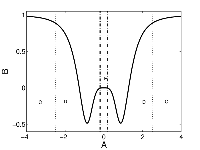
Figure 1 shows an example of a pressure gradient form factor $\hat{p}(t)$ such that if $p^{\prime(0)}(r)$ is the unperturbed pressure gradient then $p^{\prime(0)}(r)\hat{p}(t)$ is the pressure gradient with perturbation. This is the pressure flattening function that is used in Section 3. The three regions of interest can be seen in this plot: a region far from the rational surface where the pressure is not changed; a transitional region; and a region where the pressure has been completely flattened just around the rational surface. We seek to connect the outer region with the flattened region.

We now derive a second order differential equation for $\psi_{m}$ in the region $r_{a}\gg|r-r_{m}|\gg w$. This equation connects the asymptotic solutions for $\delta\gg|r-r_{m}|$, to those for $|r-r_{m}|\gg\delta$. We expand the marginal MHD equations around the surface $q=m/n$:

where the dependent variables are $y=R_{0}f\bm{\xi}.\nabla r$ and $Z=R^{2}\delta\bm{B}.\nabla\phi/B_{0}$, with $\bm{\xi}$ the plasma displacement and $\delta{\bf B}$ the perturbed magnetic field, while $Q,S,T,U,V,W,$ and $X$ are equilibrium quantities (with $T^{*}$ the complex conjugate of $T$) defined in Connor et al. [3]:

The magnetic field has been represented as

where $\phi$ is the toroidal angle, $p$ is the pressure, a prime denotes the derivative with respect to $r$, $R_{0}$ is the major radius at the magnetic axis and $B_{0}$ is the magnetic field there, following Connor et al. [3]

To facilitate the expansion we represent $q(r)\equiv\frac{m}{n}+\hat{\delta}\Delta q(t)$ where $t=(r-r_{m})/\delta$ and $\hat{\delta}=\delta/r_{m}$ and expand in $\hat{\delta}\ll 1$. ($\Delta q(t)$ is related to the perturbation $q^{(1)}(t)$ appearing in (78) by $\Delta q(t)=r_{m}tq^{(0)^{\prime}}(r_{m})+q^{(1)}(t)$.) Furthermore we write

and

In leading order $(O(\hat{\delta}^{-1}))$ (9) and (10) yield

since

and where $r$ is evaluated at $r_{m}$. These equations have solutions of the form

where $\bar{y}^{(0)}$ and $\bar{Z}^{(0)}$ contain the large and small solutions as $\Delta q\to 0$, and $\bar{\bar{y}}^{(0)}$ and $\bar{\bar{Z}}^{(0)}$ represent the regular part of the solution which is present in toroidal calculations of this nature.

Proceeding to next order in $\hat{\delta}$, i.e. $O(\hat{\delta}^{0})$, the follow equations emerge:

and

To obtain equations for $y^{(0)}$ and $Z^{(0)}$, we annihilate $y^{(1)}$ and $Z^{(1)}$ in these equations by operating with $\frac{1}{2\pi}\oint d\theta e^{-im\theta}$. The resulting equations take the following form

and

where

and we have suppressed the inhomogeneous terms involving $\bar{\bar{y}}^{(0)}$ and $\bar{\bar{Z}}^{(0)}$, since these merely determine the $m$th harmonic of the continuous solution in $\bar{y}_{0}$ and $\bar{Z}_{0}$ and do not influence the behaviour of the large and small solutions in the region adjacent to the rational surface.

To proceed further we use equilibrium relations (77), (79) and (80) to simplify the last term in (24). Thus

Finally, defining $\psi_{m}=\Delta q(t)\bar{y}^{(0)}(t)$, and eliminating $\bar{Z}^{(0)}$ from (23) and (24), we obtain a simple second order ODE for $\psi(t)$ in the form

where $K$ is independent of $t$ and is given by

or, in standard notation,

where the Mercier stability criterion [17] (for the unperturbed equilibrium) takes the form $\frac{1}{4}+D_{M\infty}>0$. We will assume that this equilibrium is Mercier stable.

We now look at (27) and find the solutions in the limits $\delta\gg|r-r_{m}|$ and $|r-r_{m}|\gg\delta$. In the limit $t\gg 1$, which is equivalently $\delta\ll|r-r_{m}|$, (27) becomes

The solution of this equation is

where we rescale to the variable $x=(r-r_{m})/r_{m}$, $\psi_{m\infty}$ is the component of the helical flux function that is resonant at $r_{m}$,

are the large and small Mercier indices respectively and $\alpha^{+,-}_{\infty}$ and $\beta^{+,-}_{\infty}$ are the coefficients of the corresponding large and small solutions to the right $(+)$ or the left $(-)$ of $r_{m}$.

In the limit $t\ll 1$, which is equivalently $\delta\gg|r-r_{m}|$, (27) becomes

The solution to this equation is

Since this is a linear problem we can write matrix equations relating $\alpha^{+,-}_{0}$ to $\alpha^{+,-}_{\infty}$ and $\beta^{+,-}_{0}$ to $\beta^{+,-}_{\infty}$ as

and

The object here is to find $\bm{M}^{+}$ and $\bm{M}^{-}$. We take $p^{\prime}(t)$ to be symmetric about $t=0$ so that $\bm{M}^{+}=\bm{M}^{-}$. The elements of $\bm{M}^{+,-}$ can be investigated by considering two basis functions at large $t$: the pure large solution $\psi_{L}(t)\sim|t|^{\nu_{L}}+...$; and the pure small solution $\psi_{S}(t)\sim|t|^{\nu_{S}}+...$. These basis functions in general generate large and small solutions at small $t$

where $c_{L},c_{S},d_{L}$ and $d_{S}$ are determined by the flattening function. The matrix $\bm{M}^{+,-}$ can then be written as

We may define $\Delta^{\prime}_{0}$ from the solutions to (27) given above in the region $t\gg 1$ as

We may also define $\Delta^{\prime}_{\infty}$ from the solutions to (27) in the region $t\gg 1$ as

where the superscripts $+(-)$ again indicate $r>r_{m}$ $(r<r_{m})$ respectively. We can link $\Delta^{\prime}_{0}$ to $\Delta^{\prime}_{\infty}$ by using (39)

If we take $\hat{\delta}$ sufficiently small that $c_{L}\gg c_{S}\frac{\beta_{\infty}}{\alpha_{\infty}}\hat{\delta}^{\nu_{S}-\nu_{L}}$ then we can write a general expression for $\Delta^{\prime}_{0}$ in terms of $\Delta^{\prime}_{\infty}$

where $u=(d_{S}c_{L}-d_{L}c_{S})/c_{L}^{2}$ and $v=d_{L}/c_{L}$ are constants depending on the perturbed quantities. Note that for $\hat{\delta}\ll 1$ and $v\neq 0$ the second term on the right hand side of (43) dominates.

Our purpose is to use analytic means to determine $\Delta^{\prime}_{\infty}$ from a numerical calculation of $\Delta^{\prime}_{0}$. In order to validate our method we will consider situations in which the solution for $t\gg 1$ can be calculated directly: numerically, as in cylindrical geometry or using the T7 code in a large aspect ratio torus.

The main result of this section is contained in (27) which describes how the large and small singular solutions behave in the vicinity of a rational surface under the influence of arbitrary localized perturbations to the safety factor and the pressure. A remarkable feature of (27) is that, although the magnetic well, or average curvature, may be modified by local currents, the Mercier index ($\beta^{\prime}_{p}K$) only responds to pressure perturbations in $\beta^{\prime(1)}_{p}$; therefore all perturbation effects cancel in $K$.

The effect on the equation for $\psi_{m}$, i.e. (27), of perturbing the pressure and current in a general torus has been calculated in the previous section. In this section we use this equation with a perturbation that flattens the pressure at the resonant surface to allow us to calculate the $\Delta^{\prime}$ for an equilibrium with pressure. Considering the situation in which there is no change in the $q$ profile, i.e. $q^{(1)}(t)=0$, (27) takes the form

where $D(t)=D_{M\infty}p^{\prime}(t)/p^{\prime}_{0}$. Bishop et al. [16] used a particular function to flatten the pressure at the rational surface.

where $r_{m}$ is the location of the rational surface, $t=(r-r_{m})/\delta$ is the local radial coordinate and, $\hat{\delta}=\delta/r_{m}\ll 1$. Solving (44) produced an analytic relationship for $u$ and $v$ in (43)

which is valid for low $\beta$ equilibria where $D_{M\infty}\ll 1$. Typically $D_{M\infty}>0$ for tokamaks with $q>1$. For $\hat{\delta}\ll 1$, $D_{M\infty}>0$ and $\Delta^{\prime}_{\infty}$ finite this yields a large negative $\Delta^{\prime}_{0}$ and stable tearing modes. Indeed $\Delta^{\prime}_{0}$ is insensitive to $\Delta^{\prime}_{\infty}$ except where $\Delta^{\prime}_{\infty}$ is very large.

In the present work we produce a new flattening function which leads to $v=0$ by carefully designing the behaviour of the large Mercier solution as it approaches the relevant mode rational surface and deducing the corresponding form of $p^{\prime}(t)$. The large solution is taken to be exactly

where the index $l$ can be chosen to produce sharper, or gentler, variations with $t$. The resulting $D(t)$ is calculated by requiring solution (47) to satisfy (44), taking $q^{(1)}(t)=0$:

Clearly, (47) has the property that a large Mercier solution approaching the mode rational surface simply changes its functional form (from $|t|^{\nu_{L}}$ to $|t|^{0}$) without changing its amplitude as it passes through the pressure flattened region, $|t|\sim O(1)$. There is no componant of the small solution in $\psi_{L}$ as $t\to 0$ i.e. $d_{L}=0$. The behaviour of the small solution is more complex. However, knowing one solution, the second solution of (44), can be constructed as

In constructing this $\psi_{S}(t)$ we have chosen a constant of integration in such a way that, as $|t|\to\infty$, $\psi_{S}$ is purely small solution. As this solution passes through the pressure flattened region it emerges, at small $t$, as a mix of large and small Mercier solutions. Specifically, for $|t|\ll 1$,

where $I_{0}(l,\nu_{L})$ is the infinite integral:

We use these results to show that $c_{L}=1$, $d_{L}=0$, $c_{S}=(2\nu_{L}-1)I_{0}$ and $d_{S}=(1-2\nu_{L})$. This leads to the following expression for the quantity $\Delta^{\prime}_{\infty}$:

This relationship has the general form (43) but importantly $v=0$ so there is no offset and $\Delta^{\prime}_{0}$ is directly proportional to $\Delta^{\prime}_{\infty}$. This direct relationship means that if $\Delta^{\prime}_{0}$ is positive so is $\Delta^{\prime}_{\infty}$. We can use (6) to show that with pressure flattening

References

- [1] La Haye R J 2006 Phys. Plasmas 13 055501
- [2] Furth H P, Killeen J, and Rosenbluth M N 1963 Phys. Fluids 6 459
- [3] Connor J W et al 1988 Phys. Fluids 31 577
- [4] Fitzpatrick R et al 1993 Nucl. Fusion, 33 1533
- [5] Cowley S C and Hastie R J 1988 Phys. Fluids, 31 426
- [6] Pletzer A and Dewar R L 1991 J. Plasma Phys. 45 427
- [7] Brennan D P et al 2002 Phys. Plasmas 9 2998
- [8] Charlton L A et al 1986 J. Comput. Phys. 63 107
- [9] Hender T C, Hastie R J, and Robinson D C 1987 Nucl. Fusion 27 1389
- [10] Liu Y Q et al 2000 Phys. Plasmas 7 3681
- [11] Ham C J et al 2012 Plasma Phys. Control. Fusion 54 105014
- [12] Newcomb W A 1960 Ann. Phys. 10 232
- [13] Glasser A H, Greene J M, and Johnson J L 1975 Phys. Fluids 18 875
- [14] Liu Y Q et al 2012 Phys. Plasmas 19 072509
- [15] Coppi B, Greene J M, and Johnson J L 1966 Nucl. Fusion 6 101
- [16] Bishop C M, Connor J W, Hastie R J, and Cowley S C 1991 Plasma Phys. Control. Fusion 33 389
- [17] Mercier C 1960 Nucl. Fusion 1 47
- [18] Ham C J et al 2012 Plasma Phys. Control. Fusion 54 025009
- [19] Greene J M and Chance M S 1981 Nucl. Fusion 21 483
- [20] Zakharov L E and Subbotin A A 1989 ITER-IL-PH-11-9-52
- [21] Westerhof E 1990 Nucl. Fusion 30 1143
- [22] Bussac M N et al 1975 Phys. Rev. Lett 35 1638