Electromagnetic Shower Properties in a Lead-Scintillator Sampling Calorimeter
Abstract
The Collider Detector at Fermilab (CDF) is a general-purpose experimental apparatus with an inner tracking detector for measuring charged particles, surrounded by a calorimeter for measurements of electromagnetic and hadronic showers. We describe a geant4 simulation and parameterization of the response of the CDF central electromagnetic calorimeter (CEM) to incident electrons and photons. The detector model consists of a detailed description of the CEM geometry and material in the direction of the incident particle’s trajectory, and of the passive material between the tracker and the CEM. We use geant4 to calculate the distributions of: the energy that leaks from the back of the CEM, the energy fraction sampled by the scintillators, and the energy dependence of the response. We parameterize these distributions to accurately model electron and photon response and resolution in a custom simulation for the measurement of the boson mass.
Keywords:
calorimeter simulation , electromagnetic shower , sampling calorimeter , energy leakage.PACS
07.05.Tp , 07.77.Ka , 07.90.+c , 29.40.-n , 29.40.Vj , 29.90.+r,
1 Introduction
The measurement of the boson mass with the CDF detector [1] at the Fermilab Tevatron collider achieves a precision of 2 parts per 10,000 on the measured energy of electrons from boson decays [2]. A key component of the energy calibration is a detailed simulation of the calorimeter response to incident electrons and photons. This simulation is based on parameterizations extracted from geant4 [3] predictions for the distributions relevant to the measurement. In this paper we describe the geant4 detector model and the parameterizations of calorimeter response and resolution.
The electron energy calibration [2] is performed in two steps. First, the calibrated track momentum (with a precision of 1 part per 10,000) is transferred to the measurement of calorimeter energy, using the distribution of the ratio of calorimeter energy to the track momentum () of electrons from the decays of and bosons. In the second step, the boson mass () is measured using electrons whose cluster energy has been calibrated with . After confirming the consistency of the measured with the world average [4], the -based calibration is combined with the -based calibration.
There are several regimes of particle type and energy relevant to this precise calorimeter calibration: the primary electron from the boson decay, with incident energy in the GeV range; radiated photons from the primary electron, with incident energies of MeV to GeV; and GeV electrons from the conversion of photons11 1 tracks with MeV curl up in the tracker’s magnetic field and do not reach the calorimeter. radiated by the primary electron. The CEM is a lead-scintillator sampling calorimeter. To simulate its response to incident electrons and photons of these energies, we parameterize the following quantities:
- •
the fraction of the incident particle’s energy that leaks out the back of the CEM;
- •
the fraction of the deposited energy sampled by the scintillators;
- •
the sampling fluctuations in the scintillator energy fraction; and
- •
the loss of response due to absorption and back-scatter of low-energy particles.
In the following we describe the detailed detector geometry implemented in geant4 (Section 2); the fractional energy leakage for a given particle type and energy (Section 3); the sampling fraction and resolution of the calorimeter (Section 4); and the absorption of energy in the passive material that results in a non-linear calorimeter response (Section 5).
2 Detector Model
The CDF detector [1, 5, 6, 7] is shown in Fig. 1. The detector model implemented in the geant4 simulation includes the components from the outer radius of the central tracking drift chamber [8] to the back end of the CEM calorimeter. These components are the outer aluminum casing of the tracker, the time-of-flight (TOF) system [9] attached to this casing, the solenoidal coil [10] that provides a nearly uniform 1.4 T magnetic field in the tracking volume, the central preshower system (CPR) [11] beyond the solenoid, and the CEM calorimeter (including longitudinal segmentation) [12].

The CEM calorimeter is divided into [13] towers, shown in Fig. 2. The tower geometry depends on , with towers numbered according to their distance in from . The longitudinal segmentation of Tower 0 is an alternating system of 31 scintillator sheets and 30 aluminum-clad lead sheets, with a plate of aluminum at the front end of the tower. Each lead sheet is 3.175 mm thick and the aluminum cladding is 380 m thick on each side of the sheet. Each scintillator sheet is 5 mm thick. A thin (6 mm) aluminum casing contains a strip and wire chamber at the position of shower maximum (after six lead-scintillator sandwiches). Almost all the material between the tracking volume and the first scintillator – the outer casing of the tracker, the solenoid coil and the CEM front plate – is aluminum. The TOF and CPR are a combination of scintillator and aluminum. Table 1 shows the materials in the geant4 model with their thicknesses in units of mm () and radiation length ().

| Material | Thickness (mm) | |
|---|---|---|
| CEM lead sheet | ||
| CEM aluminum cladding | ||
| CEM scintillator sheet | ||
| CES aluminum | 6.0 | 0.07 |
| Solenoid coil aluminum | 76.5 | 0.86 |
| CEM front-plate aluminum | 14.0 | 0.157 |
| Tracker+TOF+CPR aluminum | 27.0 | 0.303 |
We model the material between the tracking volume and the first CEM scintillator as an aluminum plate of 6.51 cm thickness plus an aluminum-clad lead sheet at the front of the active calorimeter volume. The additional lead sheet is included for simplicity: with this sheet the CEM volume is modelled as 31 alternating lead-scintillator layers. Combined, the 6.51 cm of aluminum and the single lead sheet reproduce the total radiation lengths upstream of the first scintillator layer.
The geometry of other towers is implemented according to Table 2. As increases, the number of lead sheets in a tower decreases, compensating for the increasing path length. This approximately maintains the same total number of radiation lengths traversed by a particle originating from the center of the detector. For each removed lead sheet, acryllic is used in its place and the subsequent scintillator sheet is blackened so that the sampling fraction is unaffected. In the geant4 model described here we neglect the additional radiation lengths contributed by acryllic and blackened scintillator. In the CDF measurement of the boson mass [2] a correction is applied to account for this extra plastic material.
| Tower | Thickness () | Number of lead sheets |
| 0 | 17.9 | 30 |
| 1 | 18.2 | 30 |
| 2 | 18.2 | 29 |
| 3 | 17.8 | 27 |
| 4 | 18.0 | 26 |
| 5 | 17.7 | 24 |
| 6 | 18.1 | 23 |
| 7 | 17.7 | 21 |
| 8 | 18.0 | 20 |
3 Longitudinal Leakage
The entire assembly of the lead-scintillator sandwich plus upstream material is about 18 radiation lengths thick. A typical 50 GeV incident electron will deposit about 48 GeV of its energy in this structure, and about 5% will leak out the back. The leakage energy fluctuates from shower to shower, contributing to the measurement resolution of the electron’s energy. Because this resolution is not gaussian, it is important to model the leakage distribution directly. We develop parameterizations of the energy loss distributions of incident electrons and photons as functions of incident energy and angle, and of calorimeter thickness.
3.1 Electron Leakage Model
We define the leakage fraction as the ratio of longitudinal leakage energy to the incident energy of the electron, where the incident energy is defined as the energy of the electron as it enters the outer casing of the drift chamber. Figure 3 shows the leakage fraction for three incident energies (25, 50, and 100 GeV) and for three CEM thicknesses (with 29, 30, and 31 lead-scintillator layers) for 50 GeV electrons. The distributions are skewed due to a tail that extends beyond 10%. Because of this skew it is more convenient to study the logarithm of the leakage fraction. Figure 4 shows this distribution for the same incident energies and thicknesses as Fig. 3. We find that has a nearly invariant shape, with the peak position shifting as a function of incident energy and CEM thickness. We use this feature to devise a compact parameterization of the leakage fraction.


As shown in Fig. 5 for electrons with 50 GeV of energy normally incident on Tower 0, the standard Gamma distribution gives a good description of the distribution of , with . At this energy, the parameters of the Gamma distribution are , and . Of these parameters, only depends on the incident electron energy and CEM thickness at sufficiently large energy. The following parameterization accurately models this dependence for GeV:
| (1) |
implying that a change in the incident energy by a factor of two has the same effect on the leakage energy distribution as a change in the calorimeter thickness by one radiation length.

Figures 6 and 7 show the parameterization overlaid with the geant4 simulation for electrons with energies ranging from 1 to 25 GeV. The figures show that the parameterization breaks down for electrons with GeV. To correct this deficiency, we smear the value drawn from the Gamma distribution by adding a random gaussian variable with mean and resolution , where GeV). This smearing has a progressively larger effect on the distribution of at smaller values of . The combination of the Gamma distribution with this ad-hoc smearing models the geant4 distributions well. Figures 8 to 9 show the complete parameterized model compared to the geant4 distributions.


3.2 Photon Leakage Model
For high energy photons the dominant interaction mechanism is electron-positron pair production. We model the photon shower as a photon conversion followed by the showering of the resulting electron and positron. To implement this model, we generate a random variable (in units of radiation lengths) representing the photon penetration depth before conversion. The distribution of is given by the exponential distribution [4],
| (2) |
Subtracting this value of from the total thickness of the CEM in radiation lengths gives the remaining thickness through which the electron and positron propagate. The energy of the conversion electron is obtained from the spectrum [4]
| (3) |
where is the fraction of the photon’s energy carried by the electron. Given the electron energy and the remaining calorimeter thickness, the response for the electron and positron can be simulated using the parameterizations given earlier, yielding the effective response for the original photon. Figures 8 and 9 show that this model reproduces the geant4 distributions well for incident photons.
4 Scintillator Sampling Model
To first order, the scintillation light produced by the shower is proportional to the energy deposited in the scintillator (). Defining the sampling fraction as , where is the incident energy, the leakage fluctuations cause the average to depend on . In addition, there are stochastic fluctuations in .
4.1 Leakage Dependence
We expect a positive correlation between and because showers that initiate early have relatively low and also low , since the first radiation lengths are not instrumented and the scintillator layers follow the absorber in the subsequent layers. Figure 10 shows the correlation between and for electrons (photons) for three tower geometries: Tower 0, Tower 5 (Tower 4) and Tower 8. Since the absolute value of (%) is irrelevant, we rescale for each plot such that at .
Figure 10 shows that the positive correlation between and grows as the tower rapidity increases. One reason for this increased correlation is the increasing amount of uninstrumented material in front of the calorimeter, due to oblique incidence. Since the upstream uninstrumented material causes the positive correlation, increasing the former increases the correlation. Another reason is the reduction in the number of scintillator layers, so that each scintillator contributes a larger fraction of the total signal. Showers with higher leakage have more signal deposited in the last scintillator, giving a larger positive correlation between and leakage.
The polynomial fits in Fig. 10 are used to evaluate for a given value of in the custom simulation of electron and photon showers used for the boson mass measurement at CDF [2].


4.2 Sampling Resolution
The fluctuations in correspond to the sampling resolution of the CEM, which is characterized as . Figure 11 shows the distributions of the normalized (i.e. ) at different energies. To remove the effect of leakage on the resolution, these distributions are obtained from geant4 using a very deep calorimeter with no leakage. To extract we plot the rms of each distribution as a function of incident energy. A fit to the functional form yields %. This calculation of the sampling resolution takes into account the fluctuations of the scintillator sampling fraction, but not the fluctuations of the scintillation photons and photoelectrons in the phototubes. These fluctuations contribute a sampling resolution of 7% based on the measurement of 200 photoelectrons per GeV of incident energy [12]. Combining the two sources of sampling fluctuations in quadrature yields an effective sampling term of 12.6%.

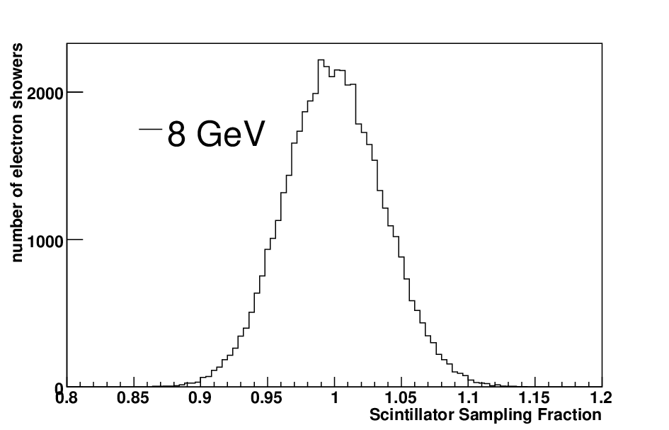

5 Sources of Non-Linearity
A source of non-linearity at high energy is the longitudinal leakage from the back of the calorimeter, since the fraction of energy that leaks increases with energy. The parameterization of longitudinal leakage was discussed in Section 3. To isolate other sources of non-linearity, we eliminate the effect of longitudinal leakage by simulating a very deep calorimeter using geant4.
A deep calorimeter is expected to be linear if on average a fixed (energy-independent) fraction of the total shower energy is deposited in the scintillator layers. In the CDF detector, the uninstrumented material upstream of the CEM absorbs energy at the start of the shower without any measurement from a corresponding scintillator sampling layer. This upstream energy loss is an important source of non-linearity.
This study encompasses several additional small sources of non-linearity. First, a non-linear effect arises from the finite thickness of the lead absorber layers. In the limit of very thin absorber layers, all shower particles generated in the absorber layers traverse the entire absorber layer and deposit some fraction of their energy in the subsequent scintillator layer. In the CEM lead layers of 3.175 mm thickness, the typical ionization energy loss for an electron is 4.1 MeV per layer at normal incidence. Soft photons that convert or Compton-scatter in the front part of a lead layer can generate lower-energy electrons which are fully absorbed in the lead, leaving no signal in the subsequent scintillator. Thus, we expect a low-energy non-linearity in the calorimeter response due to the finite thickness of the lead absorber layers.


Additional non-linearities could result from the transverse leakage of the electromagnetic shower or the back-scatter of soft photons. The bulk of the unmeasured energy from these effects will be proportional to the incident energy. However, a component of this energy loss may not scale with the incoming energy, thus causing a low-energy non-linearity.
With incident electrons and photons, we use geant4 to calculate the energy deposited in the scintillators as a function of the incident energy . We define a low-energy non-linearity parameter as
| (4) |
where represents a fixed scintilator sampling fraction. The quantity has been defined such that () is strictly proportional to . It represents an effective energy loss that can vary with energy, but we do not allow it to have a component proportional to energy, since this would simply redefine .
For this study the geant4 detector model contains a large number of layers to fully contain the shower longitudinally. In the transverse directions we define the calorimeter to have dimensions of 48 cm cm to emulate the size of a reconstructed electron cluster used in CDF data analysis [1, 7]. The geant4 prediction for is shown in Fig. 12 for incident photons and electrons. Each point in the figure is evaluated by averaging over 50,000 showers at fixed incident particle energies ranging from 5 MeV to 160 GeV. We see that is larger for photons than electrons of the same energy, and that increases logarithmically with incident energy. This increase is well-described by a function of the form
| (5) |
where is a cubic polynomial in . The scintillator sampling fraction is iteratively tuned in Eqn. 4 such that the fit returns .
The non-linearity from the dominant sources – uninstrumented material upstream of the CEM and the finite thickness of the absorber sheets – tends to increase as the incidence angle of the electron or photon moves away from normal incidence. This is because the increased path length through uninstrumented material causes more early showering and therefore more unsampled energy loss. To demonstrate this dependence on incidence angle, Fig. 12 shows as a function of energy for ranging from 1.16 to 1.82, where corresponds to normal incidence. The plots show that the energy loss increases with increasing .
6 Summary
We have implemented in geant4 the longitudinal structure of the central electromagnetic calorimeter of the CDF detector, as well as the passive material between the outer edge of the tracker and the calorimeter. Using this simulation, we calculate the longitudinal energy leakage for incident electrons as a function of incident energy and the total thickness of the structure in radiation lengths. We parameterize this distribution and derive an additional parameterization for incident photons by converting each incident photon to an electron-positron pair. We have also studied: the correlation between the energy deposited in the scintillator and the longitudinal energy leakage; the scintillator sampling fluctuations; and the calorimeter non-linearity arising from upstream passive material and finite absorber thickness. The parameterizations are used in the measurement of the boson mass with the CDF detector.
Acknowledgements
We wish to thank our colleagues on the CDF experiment for providing information on the construction of the detector. We thank Ravi Shekhar
for his assistance in installing the geant4 software.
We acknowledge the support of the U.S. Department of Energy
and the Science and Technology Facilities Council of the United Kingdom.
References
- [1] CDF Collaboration (D. Acosta et al.), Phys. Rev. D 77, 112001 (2008).
- [2] CDF Collaboration (T. Aaltonen et al.), Phys. Rev. Lett. 108, 151803 (2012).
- [3] S. Agostinelli et al., Nucl. Instrum. Meth. A506, 250 (2003); J. Allison et al., IEEE Trans. Nucl. Sci. 53 No. 1, 270 (2006).
- [4] J. Beringer et al. (Particle Data Group), Phys. Rev. D 86, 010001 (2012).
- [5] CDF Collaboration (F. Abe et al.), Nucl. Instrum. Meth. A271, 387 (1988).
- [6] CDF Collaboration (D. Acosta et al.), Phys. Rev. D 71, 032001 (2005).
- [7] CDF Collaboration (A. Abulencia et al.), J. Phys. G: Nucl. Part. Phys. 34, 2457 (2007).
- [8] T. Affolder et al., Nucl. Instrum. Meth. A 526, 249 (2004).
- [9] D. Acosta et al., Nucl. Instrum. Meth. A 518, 605 (2004).
- [10] H. Minemura et al., Nucl. Instrum. Meth. A238, 18 (1985).
- [11] A. Artikov et al., arXiv:0706.3922 (2007).
- [12] L. Balka et al., Nucl. Instrum. Meth. A267, 272 (1988).
- [13] Pseudorapidity is defined as , where is the polar angle from the beam axis. The azimuthal angle is denoted by . Energy (momentum) transverse to the beam is denoted as (). We use the convention throughout this paper.