Toric Polynomial Generators of Complex Cobordism

Andrew Wilfong

Date: August 24, 2026

Abstract.

Although it is well-known that the complex cobordism ring is a polynomial ring $\Omega_{*}^{U}\cong\mathbb{Z}\left[\alpha_{1},\alpha_{2},\ldots\right]$ , an explicit description for convenient generators $\alpha_{1},\alpha_{2},\ldots$ has proven to be quite elusive. The focus of the following is to construct complex cobordism polynomial generators in many dimensions using smooth projective toric varieties. These generators are very convenient objects since they are smooth connected algebraic varieties with an underlying combinatorial structure that aids in various computations. By applying certain torus-equivariant blow-ups to a special class of smooth projective toric varieties, such generators can be constructed in every complex dimension that is odd or one less than a prime power. A large amount of evidence suggests that smooth projective toric varieties can serve as polynomial generators in the remaining dimensions as well.

Key words and phrases:

cobordism, toric variety, blow-up, fan

2000 Mathematics Subject Classification

57R77, 14M25, 52B20

1. Introduction

In 1960, Milnor and Novikov independently showed that the complex cobordism ring $\Omega_{*}^{U}$ is isomorphic to the polynomial ring $\mathbb{Z}\left[\alpha_{1},\alpha_{2},\ldots\right]$ , where $\alpha_{n}$ has complex dimension $n$ [14, 16]. The standard method for choosing generators $\alpha_{n}$ involves taking products and disjoint unions of complex projective spaces and Milnor hypersurfaces $\mathcal{H}_{i,j}\subset\mathbb{C}P^{i}\times\mathbb{C}P^{j}$ . This method provides a smooth algebraic not necessarily connected variety in each even real dimension whose cobordism class can be chosen as a polynomial generator of $\Omega_{*}^{U}$ . Replacing the disjoint unions with connected sums give other choices for polynomial generators. However, the operation of connected sum does not preserve algebraicity, so this operation results in a smooth connected not necessarily algebraic manifold as a complex cobordism generator in each dimension.

Since Milnor and Novikov’s original construction, others have searched for more convenient choices for generators of $\Omega_{*}^{U}$ . For example, Buchstaber and Ray provided an alternate construction of polynomial generators in 1998 [3, 4]. They described certain smooth projective toric varieties which multiplicatively generate $\Omega_{*}^{U}$ . As a consequence, disjoint unions of these toric varieties can be chosen as polynomial generators. Taking connected sums instead allows one to choose a convenient topological generalization of a toric variety called a quasitoric manifold as a generator in each dimension. The advantage of these quasitoric generators is that they have a convenient combinatorial structure that aids in many computations. However, this technique still only provides examples of generators that are connected or algebraic, but not both in general.

Several years later, Johnston took a drastically different approach to constructing polynomial generators of complex cobordism which resulted in the discovery of generators that are simultaneously connected and algebraic [11]. More specifically, Johnston’s construction involves taking a sequence of blow-ups of hypersurfaces and complete intersections in smooth projective algebraic varieties, starting with complex projective space. By tracking the change of a certain cobordism invariant called the Milnor genus, Johnston proved that every complex cobordism polynomial ring generator $\alpha_{n}$ can be represented by a smooth projective connected variety.

The purpose of the following is to apply techniques similar to those of Johnston to search for even more convenient choices for complex cobordism polynomial generators, namely smooth projective toric varieties. Not only are these connected and algebraic like Johnston’s generators, but they also display the computationally-convenient combinatorial characteristics of Buchstaber and Ray’s quasitoric generators.

Conjecture 1.1.

For each $n\geq 1$ , there exists a smooth projective toric variety whose cobordism class can be chosen for the polynomial generator $\alpha_{n}$ of $\Omega_{*}^{U}\cong\mathbb{Z}\left[\alpha_{1},\alpha_{2},\ldots\right]$ .

Taking torus-equivariant blow-ups of certain smooth projective toric varieties will provide examples of such generators in most dimensions. More specifically,

Theorem 1.2.

If $n$ is odd or $n$ is one less than a power of a prime, then the cobordism class of a smooth projective toric variety can be chosen for the complex cobordism ring polynomial generator of complex dimension $n$ .

It seems very likely that generators can be found in the remaining even dimensions as well using a similar strategy. In fact, this would be a consequence of a certain number theory conjecture. Although this conjecture has not yet been verified, there is a significant amount of numerical evidence that supports it.

Theorem 1.3.

If $n\leq 100\,001$ , then the cobordism class of a smooth projective toric variety can be chosen for the complex cobordism ring polynomial generator of complex dimension $n$ .

To prove these results, it is of course essential to know when a manifold can be chosen to represent a polynomial generator of the complex cobordism ring. Detecting polynomial generators of $\Omega_{*}^{U}$ involves computing the value of a certain cobordism invariant.

Definition 1.4.

Consider a stably complex manifold $M^{2n}$ , and formally write it Chern class as $c\left(M\right)=\prod\limits_{k=1}^{n}\left(1+x_{k}\right)$ . The Milnor genus $s_{n}\left[M\right]$ of $M$ is the characteristic number obtained by evaluating the cohomology class $s_{n}\left(c\left(M\right)\right)=\sum\limits_{k=1}^{n}x_{k}^{n}$ on the fundamental class of $M$ , i.e.

s_{n}\left[M\right]=\left\langle\sum_{k=1}^{n}x_{k}^{n},\mu_{M}\right\rangle\in\mathbb{Z}.

Milnor and Novikov proved that $\left[M^{2n}\right]$ can be chosen for the polynomial generator $\alpha_{n}$ of $\Omega_{*}^{U}\cong\mathbb{Z}\left[\alpha_{1},\alpha_{2},\ldots\right]$ if and only if the following relation holds:

(1)

s_{n}\left[M^{2n}\right]=\begin{cases}\pm 1&\mbox{ if }n+1\neq p^{m}\mbox{ for any prime }p\mbox{ and integer }m\\ \pm p&\mbox{ if }n+1=p^{m}\mbox{ for some prime }p\mbox{ and integer }m\end{cases}

(see [15] for details).

The focus of this paper is to construct smooth projective toric varieties whose Milnor genera have the appropriate value in order for the variety to be chosen for the polynomial generators $\alpha_{n}$ of complex cobordism. Section 2 offers a brief introduction to toric varieties and their pertinent topological properties. It also includes the construction of certain smooth projective toric varieties $Y_{n}^{\varepsilon}\left(a,b\right)$ which are used in later sections to construct complex cobordism polynomial generators. Section 3 proves the existence of smooth projective toric variety polynomial generators in even complex dimensions one less than a prime power. In Section 4, such generators are found in all odd dimensions. In Section 5, the remaining unproven dimensions are discussed. More specifically, a number-theoretic conjecture is presented which is sufficient to verify the existence of smooth projective toric variety polynomial generators in the remaining dimensions. Overwhelming numerical evidence is given in support of this conjecture.

The established methods of Milnor, Novikov, Buchstaber, and Ray for producing complex cobordism polynomial generators do not provide an explicit universal description of generators, as their methods rely on solving certain Diophantine equations. The techniques in this paper and those of Johnston [11] still do not provide this desirable universal description in most dimensions, since the constructions involve finding a sequence of blow-ups of unspecified length. Section 6 discusses the possibility of finding a convenient, explicit description of complex cobordism polynomial generators among smooth projective toric varieties.

2. Toric Varieties

A toric variety is a normal variety that contains the torus as a dense open subset such that the action of the torus on itself extends to an action on the entire variety. Remarkably, these varieties are in one-to-one correspondence with objects from convex geometry called fans. Therefore, studying the combinatorial properties of these fans can reveal a great deal of information about the corresponding toric varieties. See [8, 5] for a more in-depth treatment of toric varieties.

Definition 2.1.

A (strongly convex rational polyhedral) cone $\sigma$ spanned by generating rays $v_{1},\ldots,v_{m}\in\mathbb{Z}^{n}$ is a set of points

\sigma=\mbox{pos}\left(v_{1},\ldots,v_{m}\right)=\left\{\sum\limits_{k=1}^{m}a_{k}v_{k}\in\mathbb{R}^{n}\Bigr|a_{k}\geq 0\right\}

such that $\sigma$ does not contain any lines passing through the origin.

A fan $\Delta$ in $\mathbb{R}^{n}$ is a set of cones in $\mathbb{R}^{n}$ such that each face of a cone in $\Delta$ also belongs to $\Delta$ , and the intersection of any two cones in $\Delta$ is a face of both cones.

The one-dimensional cones of a fan are called its generating rays.

A cone can be used to construct a $\mathbb{C}$ -algebra which is the coordinate ring of an affine toric variety. A fan can in turn be used to construct an abstract toric variety. More specifically, if two cones $\sigma_{1}$ and $\sigma_{2}$ of a fan intersect at a face $\tau$ , then the affine varieties $U_{\sigma_{1}}$ and $U_{\sigma_{2}}$ of the two cones can be glued together along the subvariety $U_{\tau}$ associated to $\tau$ to produce a toric variety associated to the fan $\sigma_{1}\cup\sigma_{2}$ . This construction demonstrates that every fan defines a corresponding toric variety. In fact, the converse is also true.

Theorem 2.2.

([5, Section 3.1]) There is a bijective correspondence between equivalence classes of fans in $\mathbb{R}^{n}$ under unimodular transformations and isomorphism classes of complex $n$ -dimensional toric varieties.

The fan corresponding to a variety $X$ will be denoted $\Delta_{X}$ , and the variety corresponding to a fan $\Delta$ will be denoted $X_{\Delta}$ . This bijection can be proven by examining the orbits of a toric variety under the torus action. There is a bijective correspondence between these orbits and the cones of the associated fan.

Theorem 2.3.

([5, Section 3.2]) Consider a fan $\Delta$ in $\mathbb{R}^{n}$ and its associated complex dimension $n$ toric variety $X_{\Delta}$ . Every orbit of the torus action on $X_{\Delta}$ corresponds to a distinct cone in $\Delta$ . If such an orbit is a $k$ -dimensional torus, then the corresponding cone will have dimension $n-k$ .

As a result of this correspondence between fans and toric varieties, many of the algebraic properties of toric varieties directly correspond to properties of the associated fans.

Proposition 2.4.

([13]) Consider a fan $\Delta$ in $\mathbb{R}^{n}$ .

The toric variety $X_{\Delta}$ is compact if and only if $\Delta$ is a complete fan, i.e. the union of all of the cones in $\Delta$ is $\mathbb{R}^{n}$ itself.

The variety is smooth if and only if $\Delta$ is regular, i.e. every maximal $n$ -dimensional cone is spanned by $n$ generating rays that form an integer basis.

The variety $X_{\Delta}$ is isomorphic to the variety $X_{\Delta^{\prime}}$ if and only if there is a unimodular transformation $\mathbb{Z}^{n}\rightarrow\mathbb{Z}^{n}$ which maps $\Delta$ into $\Delta^{\prime}$ and preserves the simplicial structure of the fans.

The variety $X_{\Delta}$ is projective if and only if $\Delta$ is normal to a lattice polytope (see [2, Section 5.1] for details about polytopes and their relation to toric varieties).

The convenient combinatorial structure of a fan can also be used to determine many important topological properties of the corresponding toric varieties. For example, Jurkiewicz computed the integral cohomology ring of a smooth projective toric variety, and Danilov generalized the result to all smooth toric varieties.

Consider a complete regular fan $\Delta$ in $\mathbb{R}^{n}$ with generating rays $v_{1},\ldots,v_{m}$ . Each of the rays $v_{k}$ is a one-dimensional cone in $\Delta$ which corresponds to a codimension two subvariety $X_{k}$ of $X_{\Delta}$ . Each of these subvarieties determines a cohomology class in $H^{2}\left(X_{\Delta}\right)$ by taking the image of the fundamental class $\left[X_{k}\right]$ of $X_{k}$ under the composition

H_{2n-2}\left(X_{k}\right)\hookrightarrow H_{2n-2}\left(X_{\Delta}\right)\rightarrow H^{2}\left(X_{\Delta}\right),

where the first map is induced from inclusion and the second is Poincaré duality. Denote the cohomology class in $H^{2}\left(X_{\Delta}\right)$ corresponding to the ray $v_{k}$ by $v_{k}$ as well. It will be clear from context what the meaning of $v_{k}$ is.

Theorem 2.5.

([12, 6]) Suppose the generating rays $v_{1},\ldots,v_{m}$ of a complete regular fan $\Delta$ in $\mathbb{R}^{n}$ are given by $v_{j}=\left(\lambda_{1j},\ldots,\lambda_{nj}\right)$ . For $i=1,\ldots,n$ , set

\theta_{i}=\lambda_{i1}v_{1}+\ldots+\lambda_{im}v_{m}\in\mathbb{Z}\left[v_{1},\ldots,v_{m}\right].

Define $L=\left(\theta_{1},\ldots,\theta_{n}\right)$ to be the ideal generated by these linear polynomials. Also define $J$ to be the ideal generated by all square-free monomials $v_{i_{1}}\cdots v_{i_{k}}$ such that $v_{i_{1}},\ldots,v_{i_{k}}$ do not span a cone in $\Delta$ (the Stanley-Reisner ideal of $\Delta$ ). Then the integral cohomology of the toric variety $X_{\Delta}$ is given by

H^{*}\left(X_{\Delta}\right)\cong\mathbb{Z}\left[v_{1},\ldots,v_{m}\right]/\left(L+J\right).

The Chern class of a smooth toric variety can also be computed using combinatorial data. The natural complex structure of a smooth toric variety leads to a stable splitting of its tangent bundle, and this splitting is encoded in the fan associated to the toric variety.

Theorem 2.6.

(see [2, Section 5.3] for details) Given a complete regular fan $\Delta$ in $\mathbb{R}^{n}$ with generating rays $v_{1},\ldots,v_{m}$ , the total Chern class of $X_{\Delta}$ is given by

c\left(X_{\Delta}\right)=\left(1+v_{1}\right)\left(1+v_{2}\right)\cdots\left(1+v_{m}\right)\in H^{*}\left(X_{\Delta}\right).

This splitting of the Chern class leads to a description of the Milnor genus of a smooth toric variety in terms of its fan.

Corollary 2.7.

Let $X_{\Delta}$ be a smooth toric variety corresponding to a complete regular fan $\Delta$ in $\mathbb{R}^{n}$ with generating rays $v_{1},\ldots,v_{m}$ . Then the Milnor genus of $X_{\Delta}$ is given by

s_{n}\left[X_{\Delta}\right]=\left\langle\sum_{k=1}^{m}v_{k}^{n},\mu_{X_{\Delta}}\right\rangle.

Unfortunately, this formula is usually difficult to evaluate in most cohomology rings of smooth toric varieties. The following proposition is particularly useful in attempting these evaluations of characteristic numbers.

Proposition 2.8.

([8, Section 5.1]) Suppose $\mbox{pos}\left(v_{1},\ldots,v_{n}\right)$ is a maximal cone of a complete regular fan $\Delta$ in $\mathbb{R}^{n}$ . Then evaluating $v_{1}\cdots v_{n}\in H^{2n}\left(X_{\Delta}\right)$ on the fundamental class $\mu_{X_{\Delta}}$ of the variety yields one, i.e.

\left\langle v_{1}\cdots v_{n},\mu_{X_{\Delta}}\right\rangle=1.

The blow-up $\mbox{Bl}_{V}X$ of a variety $X$ along a subvariety $V$ can also be described using fans in the case of toric varieties (see [9, Chapter 1 Section 4 and Chapter 4 Section 6] for details about blow-ups). Consider a complete regular fan $\Delta$ in $\mathbb{R}^{n}$ containing a cone $\sigma$ of dimension $k$ . Then there are $k$ -many generating rays $v_{1},\ldots,v_{k}$ of $\Delta$ such that $\sigma=\mbox{pos}\left(v_{1},\ldots,v_{k}\right)$ . Construct a new fan $\mbox{Bl}_{\sigma}\Delta$ by first introducing a new generating ray $x=v_{1}+\ldots+v_{k}$ . To obtain the cones of $\mbox{Bl}_{\sigma}\Delta$ , first keep all cones in $\Delta$ that do not contain $\sigma$ . Any cone $\tau$ in $\Delta$ that contains $\sigma$ is no longer one of the cones in $\mbox{Bl}_{\sigma}\Delta$ . These cones $\tau$ in $\Delta$ of the form $\tau=\mbox{pos}\left(v_{1},\ldots,v_{k},v_{i_{1}},\ldots,v_{i_{j}}\right)$ are removed from $\mbox{Bl}_{\sigma}\Delta$ and replaced with all cones of the form $\mbox{pos}\left(v_{1},\ldots,\hat{v}_{l},\ldots,v_{k},x,v_{i_{1}},\ldots,v_{i_{j}}\right)$ . That is, one of the rays of $\sigma$ is removed and replaced with $x$ to obtain a new cone in $\mbox{Bl}_{\sigma}\Delta$ . The fan $\mbox{Bl}_{\sigma}\Delta$ is called the star subdivision of $\Delta$ relative to $\sigma$ (see [5, Section 3.3] for details).

Proposition 2.9.

([5, Section 3.3]) Let $\Delta$ be a complete regular fan in $\mathbb{R}^{n}$ . Consider a $k$ -dimensional cone $\sigma=\mbox{pos}\left(v_{1},\ldots,v_{k}\right)$ in $\Delta$ , and let $X_{\sigma}$ denote the $\left(n-k\right)$ -dimensional toric subvariety of $X_{\Delta}$ which is associated to the cone $\sigma$ . Then $X_{\mbox{\emph{Bl}}_{\sigma}\Delta}=\mbox{\emph{Bl}}_{X_{\sigma}}X_{\Delta}$ . That is, the blow-up of $X_{\Delta}$ along the subvariety $X_{\sigma}$ is a toric variety whose associated fan is the star subdivision of $\Delta$ relative to $\sigma$ .

The operation of blowing up along torus-equivariant subvarieties preserves several key properties of toric varieties. The following proposition is well-known.

Proposition 2.10.

The blow-up of a smooth projective toric variety along a subvariety that is an orbit of the torus action is itself a smooth projective toric variety.

It is straight-forward to verify that the blow-up is smooth by computing determinants of the maximal cones resulting from the star subdivision. The fan of the blown up variety is normal to a polytope obtained by truncating the polytope associated to the original variety along the face corresponding to the cone being blown up. The resulting polytope has vertices with rational coefficients. Dilating this polytope produces a lattice polytope, so the blown up variety, whose fan is normal to this polytope, is also projective.

In general, the complexity of the cohomology ring makes it challenging to compute the Milnor genus of a smooth toric variety using Corollary 2.7. However, by carefully choosing toric varieties with a convenient bundle structure and taking certain blow-ups, one obtains a collection of smooth projective toric varieties that are simple enough to allow their Milnor genera to be computed yet still complicated enough to produce a wide array of possible values for these Milnor genera. These varieties can be used to find complex cobordism polynomial generators in most dimensions, and it seems likely that they can be used as generators in every dimension.

Definition 2.11.

Fix a complex dimension $n\geq 3$ , an integer $\varepsilon\in\left\{2,\ldots,n-1\right\}$ , and two integers $a$ and $b$ . Define $U=\left\{u_{1},\ldots,u_{n-\varepsilon+1}\right\}$ , where $u_{k}=e_{k}$ is the standard basis vector in $\mathbb{R}^{n}$ for $k=1,\ldots,n-\varepsilon$ , and set $u_{n-\varepsilon+1}=\left(-1,\stackrel{{\scriptstyle\left(n-\varepsilon\right)}}{{\ldots}},-1,0,\ldots,0\right)$ . Also define $V=\left\{v_{1},\ldots,v_{\varepsilon}\right\}$ , where $v_{k}=e_{n-\varepsilon+k}$ is the standard basis vector for $k=1,\ldots,\varepsilon-1$ , and $v_{\varepsilon}=\left(0,\stackrel{{\scriptstyle\left(n-\varepsilon-1\right)}}{{\ldots\ldots}},0,a,-1,\ldots,-1,0\right)$ . Finally, define $W=\left\{w_{1},w_{2}\right\}$ , where $w_{1}=e_{n}$ and $w_{2}=\left(0,\ldots,0,b,-1\right)$ . A fan $\Delta_{n}^{\varepsilon}\left(a,b\right)$ in $\mathbb{R}^{n}$ can be defined by using the $\left(n+3\right)$ -many generating rays in $U\cup V\cup W$ . A maximal cone in $\Delta_{n}^{\varepsilon}\left(a,b\right)$ is obtained by choosing for generators $\left(n-\varepsilon\right)$ -many vectors from $U$ , $\left(\varepsilon-1\right)$ -many vectors from $V$ , and $1$ vector from $W$ . Let $Y_{n}^{\varepsilon}\left(a,b\right)$ denote the toric variety corresponding to this fan.

It is easy to verify that $\Delta_{n}^{\varepsilon}\left(a,b\right)$ is a complete regular fan that is normal to a lattice polytope. Therefore, $Y_{n}^{\varepsilon}\left(a,b\right)$ is a compact smooth projective toric variety. More specifically, $\Delta_{n}^{\varepsilon}\left(a,b\right)$ can be viewed as the join of three separate fans $\Delta_{U}$ , $\Delta_{V}$ , and $\Delta_{W}$ whose generating rays belong to $U$ , $V$ , and $W$ , respectively (see Figure 1). On the level of toric varieties, $Y_{n}^{\varepsilon}\left(a,b\right)$ is a stack of two projectivized bundles. More specifically, the toric variety corresponding to $\Delta_{V}*\Delta_{W}$ is a $\mathbb{C}P^{\varepsilon-1}$ -bundle over $X_{\Delta_{W}}\cong\mathbb{C}P^{1}$ . The variety $Y_{n}^{\varepsilon}\left(a,b\right)$ is a $\mathbb{C}P^{n-\varepsilon}$ -bundle over the variety corresponding to $\Delta_{V}*\Delta_{W}$ . Refer to [5, Section 3.3] for more details about obtaining fiber bundle structures from fans such as these.

Refer to caption — Figure 1. $\Delta_{n}^{\varepsilon}\left(a,b\right)$ depicted as a join of fans

The bundle structure of $Y_{n}^{\varepsilon}\left(a,b\right)$ makes it convenient to calculate its cohomology ring and Milnor genus.

Proposition 2.12.

Fix a complex dimension $n$ , an integer $\varepsilon\in\left\{2,\ldots,n-1\right\}$ and two integers $a$ and $b$ . Define $R_{n}\left(\varepsilon\right)=n-\varepsilon+\left(-1\right)^{\varepsilon}{n-1\choose\varepsilon}$ . The Milnor genus of $Y_{n}^{\varepsilon}\left(a,b\right)$ is given by

s_{n}\left[Y_{n}^{\varepsilon}\left(a,b\right)\right]=a^{\varepsilon}bR_{n}\left(\varepsilon\right).

Proof.

By Theorem 2.5,

H^{*}\left(Y_{n}^{\varepsilon}\left(a,b\right)\right)\cong\mathbb{Z}\left[u_{1},\ldots,u_{n-\varepsilon+1},v_{1},\ldots,v_{\varepsilon},w_{1},w_{2}\right]/\left(L+J\right)

where

	$\displaystyle L$	$\displaystyle=\bigl(u_{1}-u_{n-\varepsilon+1},\ldots,u_{n-\varepsilon-1}-u_{n-\varepsilon+1},u_{n-\varepsilon}-u_{n-\varepsilon+1}+av_{\varepsilon},$
		$\displaystyle\ \ \ \ \ \ \ v_{1}-v_{\varepsilon},\ldots,v_{\varepsilon-2}-v_{\varepsilon},v_{\varepsilon-1}-v_{\varepsilon}+bw_{2},w_{1}-w_{2}\bigl)$

and $J=\left(u_{1}\cdots u_{n-\varepsilon+1},v_{1}\cdots v_{\varepsilon},w_{1}\cdot w_{2}\right)$ . Let $u,v,w\in H^{*}\left(Y_{n}^{\varepsilon}\left(a,b\right)\right)$ denote the cohomology classes corresponding to the generating rays $u_{n-\varepsilon+1},\ v_{\varepsilon}$ , and $w_{2}$ , respectively. Then the cohomology ring of $Y_{n}^{\varepsilon}\left(a,b\right)$ simplifies to become

H^{*}\left(Y_{n}^{\varepsilon}\left(a,b\right)\right)\cong\mathbb{Z}\left[u,v,w\right]/\left(u^{n-\varepsilon+1}-au^{n-\varepsilon}v,v^{\varepsilon}-bv^{\varepsilon-1}w,w^{2}\right).

The Milnor genus of $Y_{n}^{\varepsilon}\left(a,b\right)$ can be computed by first evaluating

s_{n}\left(c\left(Y_{n}^{\varepsilon}\left(a,b\right)\right)\right)=u_{1}^{n}+\ldots+u_{n-\varepsilon+1}^{n}+v_{1}^{n}+\ldots+v_{\varepsilon}^{n}+w_{1}^{n}+w_{2}^{n}

in this ring. Doing so yields

s_{n}\left(c\left(Y_{n}^{\varepsilon}\left(a,b\right)\right)\right)=a^{\varepsilon}b\left(n-\varepsilon+\left(-1\right)^{\varepsilon}{n-1\choose\varepsilon}\right)u^{n-\varepsilon}v^{\varepsilon-1}w.

Since $\mbox{pos}\left(u_{1},\ldots,u_{n-\varepsilon-1},u_{n-\varepsilon+1},v_{1},\ldots,v_{\varepsilon-2},v_{\varepsilon},w_{2}\right)$ is a maximal cone in $\Delta_{n}^{\varepsilon}\left(a,b\right)$ and we have the relation $u_{1}\cdots u_{n-\varepsilon-1}\cdot u_{n-\varepsilon+1}\cdot v_{1}\cdots v_{\varepsilon-2}\cdot v_{\varepsilon}\cdot w_{2}=u^{n-\varepsilon}v^{\varepsilon-1}w$ in $H^{*}\left(Y_{n}^{\varepsilon}\left(a,b\right)\right)$ , we have $\left\langle u^{n-\varepsilon}v^{\varepsilon-1}w,\mu_{Y_{n}^{\varepsilon}\left(a,b\right)}\right\rangle=1$ by Proposition 2.8. Then

s_{n}\left[Y_{n}^{\varepsilon}\left(a,b\right)\right]=a^{\varepsilon}b\left(n-\varepsilon+\left(-1\right)^{\varepsilon}{n-1\choose\varepsilon}\right)=a^{\varepsilon}bR_{n}\left(\varepsilon\right).

∎

As will be seen in the next section, the smooth projective toric varieties $Y_{n}^{\varepsilon}\left(a,b\right)$ provide examples of polynomial ring generators of $\Omega_{*}^{U}$ in a limited number of dimensions. To obtain examples of toric variety generators in more dimensions, we can apply certain blow-ups to these varieties. The most basic and useful of these blow-ups is the blow-up at a torus-fixed point. It is straight-forward to calculate the change in Milnor genus during this operation.

Proposition 2.13.

(cf. [11, Lemma 3.4]) Consider a complex manifold $M^{2n}$ and its blow-up $Bl_{x}M$ at $x\in M$ . The change in Milnor genus is given by the following formula.

s_{n}\left[Bl_{x}M\right]=\begin{cases}s_{n}\left[M\right]-\left(n+1\right)&\mbox{ if }n\mbox{ is even}\\ s_{n}\left[M\right]-\left(n-1\right)&\mbox{ if }n\mbox{ is odd}\end{cases}

Proof.

This formula is a consequence of the well-known fact that $Bl_{x}M$ is diffeomorphic to $M\#\overline{\mathbb{C}P^{n}}$ as an oriented differentiable manifold, where $\overline{\mathbb{C}P^{n}}$ is the complex projective space with the opposite of the standard orientation (see [10, Proposition 2.5.8] for details). We can compute $s_{n}\left[\overline{\mathbb{C}P^{n}}\right]=-\left(n+\left(-1\right)^{n}\right)$ , which gives the desired formula. ∎

3. Toric Polynomial Generators in Some Even Dimensions

The smooth projective toric varieties $Y_{n}^{\varepsilon}\left(a,b\right)$ provide examples of polynomial generators of $\Omega_{*}^{U}$ in certain dimensions. For example, the following theorem is an immediate consequence of Proposition 2.12.

Theorem 3.1.

If $n=p-1$ for some prime $p\geq 5$ , then the smooth projective toric variety $Y_{n}^{n-2}\left(1,1\right)$ can be chosen to represent the generator $\alpha_{n}$ of $\Omega_{*}^{U}\cong\mathbb{Z}\left[\alpha_{1},\alpha_{2},\ldots\right]$ .

Remark 3.2.

There are likely to be a wide array of different smooth projective toric varieties that can be chosen as polynomial generators. For example, if $n=p-1$ for some prime $p$ , then $s_{n}\left[\mathbb{C}P^{n}\right]=p$ . Thus the simpler toric variety $\mathbb{C}P^{n}$ can be chosen to represent the generator $\alpha_{n}$ of $\Omega_{*}^{U}\cong\mathbb{Z}\left[\alpha_{1},\alpha_{2},\ldots\right]$ . In fact, it is easy to show that $\mathbb{C}P^{n}$ is not cobordant to $Y_{n}^{n-2}\left(1,1\right)$ , so there are at least two distinct toric polynomial generators in dimensions that are one less than a prime $p\geq 5$ .

Theorem 3.1 can be generalized to dimensions one less than a power of an odd prime by examining blow-ups of the $Y_{n}^{\varepsilon}\left(a,b\right)$ . In this situation, a cobordism class must have Milnor genus $\pm p$ for it to be used as a polynomial generator in the complex cobordism ring (see (1)). Recall that each blow-up at a point in this even complex dimension decreases the Milnor genus by $n+1=p^{m}$ by Proposition 2.13. This means that in order to find a smooth projective toric variety with Milnor genus $p$ , it suffices to find one whose Milnor genus is positive and is congruent to $p$ modulo $p^{m}$ . The extra multiples of $p^{m}$ can then be removed by a sequence of blow-ups at points. By choosing these points to be torus-fixed points, each successive blow-up is itself a smooth projective toric variety.

A technical lemma is needed to show that some of the $Y_{n}^{\varepsilon}\left(a,b\right)$ satisfy the desired congruence in these dimensions.

Lemma 3.3.

Let $n=p^{m}-1$ for some odd prime $p$ and integer $m\geq 2$ . Then

R_{n}\left(p^{m-1}\right)\equiv-p\mbox{ mod }p^{m}\mbox{ and }R_{n}\left(p^{m-1}\right)<0,

where as in Proposition 2.12, $R_{n}\left(p^{m-1}\right)=n-p^{m-1}-{n-1\choose p^{m-1}}$ .

Proof.

To prove that $R_{n}\left(p^{m-1}\right)\equiv-p\mbox{ mod }p^{m}$ , first consider ${n-1\choose p^{m-1}}\mbox{ mod }p^{m}$ . We can write

	$\displaystyle{n-1\choose p^{m-1}}$	$\displaystyle={p^{m}-2\choose p^{m-1}}$
(2)		$\displaystyle{n-1\choose p^{m-1}}$	$\displaystyle=\frac{p^{m}-2}{2}\cdot\frac{p^{m}-3}{3}\cdots\frac{p^{m}-p^{m-1}}{p^{m-1}}\cdot\left(p^{m}-\left(p^{m-1}+1\right)\right).$

In general, if $p\not|c$ , then $c$ has a multiplicative inverse $c^{-1}$ in the multiplicative group of integers $\mathbb{Z}_{p^{m}}^{\times}$ . In this situation,

\frac{p^{m}-c}{c}=c^{-1}\left(p^{m}-c\right)\equiv-1\mbox{ mod }p^{m}.

If $p|c$ , then this cancellation cannot be applied. Applying these cancellations to (2) yields

	$\displaystyle{n-1\choose p^{m-1}}$	$\displaystyle\equiv\frac{p^{m}-p}{p}\cdot\frac{p^{m}-2p}{2p}\cdots\frac{p^{m}-p^{m-1}}{p^{m-1}}\cdot\left(p^{m-1}+1\right)\mbox{ mod }p^{m}$
		$\displaystyle\equiv\frac{p^{m-1}-1}{1}\cdot\frac{p^{m-1}-2}{2}\cdots\frac{p^{m-1}-p^{m-2}}{p^{m-2}}\cdot\left(p^{m-1}+1\right)\mbox{ mod }p^{m}.$

Applying this same cancellation procedure repeatedly eventually produces

	$\displaystyle{n-1\choose p^{m-1}}$	$\displaystyle\equiv\frac{p^{2}-1}{1}\cdot\frac{p^{2}-2}{2}\cdots\frac{p^{2}-p}{p}\cdot\left(p^{m-1}+1\right)\mbox{ mod }p^{m}$
		$\displaystyle\equiv p-p^{m-1}-1\mbox{ mod }p^{m}.$

Then $R_{n}\left(p^{m-1}\right)\equiv p^{m}-1-p^{m-1}-\left(p-p^{m-1}-1\right)\equiv-p\mbox{ mod }p^{m}$ .

To see that $R_{n}\left(p^{m-1}\right)$ is negative, note that for any integer $n\geq 3^{2}-1=8$ (the smallest possible dimension for this lemma), $n<{n-1\choose 2}$ . Then given any $p^{m}$ where $p$ is prime and $m\geq 2$ , $n=p^{m}-1<{p^{m}-2\choose 2}<{p^{m}-2\choose p^{m-1}}$ . Then $R_{n}\left(p^{m-1}\right)=p^{m}-1-p^{m-1}-{p^{m}-2\choose p^{m-1}}<0$ . ∎

Theorem 3.4.

If $n=p^{m}-1$ for some odd prime $p$ and some integer $m\geq 2$ , then there exists a smooth projective toric variety whose cobordism class can be chosen for the polynomial generator $\alpha_{n}$ of $\Omega_{*}^{U}=\mathbb{Z}\left[\alpha_{1},\alpha_{2},\ldots\right]$ .

Proof.

Consider the smooth projective toric variety $Y_{n}^{p^{m-1}}\left(1,-1\right)$ . By Proposition 2.12 and Lemma 3.3,

s_{n}\left[Y_{n}^{p^{m-1}}\left(1,-1\right)\right]=-1\cdot R_{n}\left(p^{m-1}\right)\equiv p\mbox{ mod }p^{m}\mbox{ and }s_{n}\left[Y_{n}^{p^{m-1}}\left(1,-1\right)\right]\geq p.

Since each blow-up at a point decreases the Milnor genus by $n+1=p^{m}$ (by Proposition 2.13), applying sufficiently many blow-ups to torus-fixed points of $Y_{n}^{p^{m-1}}\left(1,-1\right)$ will produce a smooth projective toric variety with Milnor genus $p$ . The cobordism class of this variety can be used as a polynomial generator of $\Omega_{*}^{U}$ by (1).∎

Example 3.5.

Suppose $n=5^{2}-1=24$ . Then

s_{24}\left[Y_{24}^{5}\left(1,-1\right)\right]=-R_{24}\left(5\right)=33630\equiv 5\mbox{ mod }25.

Each blow-up of a point in this dimension decreases the Milnor genus by $n+1=25$ . By applying a sequence of $1345$ many blow-ups at torus-fixed points to $Y_{24}^{5}\left(1,-1\right)$ , one obtains a smooth projective toric variety with Milnor genus $5$ . The cobordism class of this variety can be used as the polynomial generator $\alpha_{24}$ of $\Omega_{*}^{U}=\mathbb{Z}\left[\alpha_{1},\alpha_{2},\ldots\right]$ by (1).

This example demonstrates that although Theorem 3.4 verifies the existence of smooth projective toric variety polynomial generators in certain dimensions, the theorem is not very useful in explicitly constructing such examples.

4. Toric Polynomial Generators in Odd Dimensions

A limited number of odd-dimensional generators can be chosen from the $Y_{n}^{\varepsilon}\left(a,b\right)$ themselves. The following theorem is a direct consequence of Proposition 2.12.

Theorem 4.1.

If $n=2^{m}-1$ for some integer $m\geq 2$ , then the smooth projective toric variety $Y_{n}^{n-1}\left(1,1\right)$ can be chosen to represent the generator $\alpha_{n}$ of $\Omega_{U}^{*}\cong\mathbb{Z}\left[\alpha_{1},\alpha_{2},\ldots\right]$ .

Smooth projective toric variety cobordism generators can be obtained in the remaining odd dimensions by considering certain blow-ups. First, a simple number theory fact is needed.

Lemma 4.2.

Let $n$ be a positive odd integer. If $n\neq 2^{k}-1$ for any $k\in\mathbb{Z}$ , then

n\equiv 2^{m}-1\mbox{ mod }2^{m+1}

for some integer $m\geq 1$ .

Proof.

Suppose $n$ is odd and $n\neq 2^{k}-1$ for any $k\in\mathbb{Z}$ . Then $n+1=2^{m}\cdot q$ , where $m\geq 1$ , $q>1$ , and $2\not|q$ . Then $n+1-2^{m}=2^{m}\left(q-1\right)$ , and $q-1$ is even. Then $2^{m+1}|\left(n+1-2^{m}\right)$ , so $n\equiv 2^{m}-1\mbox{ mod }2^{m+1}$ . ∎

In order to obtain smooth projective toric variety polynomial generators of $\Omega_{*}^{U}$ in the remaining odd dimensions, we must first blow up a particular two-dimensional subvariety of $Y_{n}^{\varepsilon}\left(a,b\right)$ . The change in Milnor genus during this blow-up can be determined.

Lemma 4.3.

Fix an odd complex dimension $n\geq 3$ . Let $a$ , $b$ , and $\varepsilon$ be arbitrary integers such that $\varepsilon\in\left\{2,\ldots,n-1\right\}$ . Consider the cone $\sigma=\mbox{pos}\left(u_{1},\ldots,u_{n-\varepsilon},v_{1},\ldots,v_{\varepsilon-1}\right)$ in $\Delta_{n}^{\varepsilon}\left(a,b\right)$ of dimension $n-1$ . This cone corresponds to a real dimension two subvariety $X_{\sigma}$ of $Y_{n}^{\varepsilon}\left(a,b\right)$ . If $Y_{n}^{\varepsilon}\left(a,b\right)$ is blown up along $X_{\sigma}$ , then the Milnor genus of the resulting smooth projective toric variety $\mbox{\emph{Bl}}_{X_{\sigma}}Y_{n}^{\varepsilon}\left(a,b\right)$ is given by

s_{n}\left[\mbox{\emph{Bl}}_{X_{\sigma}}Y_{n}^{\varepsilon}\left(a,b\right)\right]=s_{n}\left[Y_{n}^{\varepsilon}\left(a,b\right)\right]+2b.

Proof.

Let $x=\left(1,\ldots,1,0\right)$ be the additional generating ray obtained when finding the star subdivision of $\Delta_{n}^{\varepsilon}\left(a,b\right)$ relative to $\sigma$ . By Theorem 2.5,

H^{*}\left(\mbox{Bl}_{X_{\sigma}}Y_{n}^{\varepsilon}\left(a,b\right)\right)\cong\mathbb{Z}\left[u_{1},\ldots,u_{n-\varepsilon+1},v_{1},\ldots,v_{\varepsilon},w_{1},w_{2},x\right]/\left(L+J\right)

where

	$\displaystyle L$	$\displaystyle=\bigl(u_{1}-u_{n-\varepsilon+1}+x,\ldots,u_{n-\varepsilon-1}-u_{n-\varepsilon+1}+x,u_{n-\varepsilon}-u_{n-\varepsilon+1}+av+x,$
		$\displaystyle\ \ \ \ \ \ \ v_{1}-v_{\varepsilon}+x,\ldots,v_{\varepsilon-2}-v_{\varepsilon}+x,v_{\varepsilon-1}-v_{\varepsilon}+bw+x,w_{1}-w_{2}\bigl)$

and

J=\left(u_{1}\cdots u_{n-\varepsilon+1},v_{1}\cdots v_{\varepsilon},w_{1}\cdot w_{2},u_{1}\cdots u_{n-\varepsilon}\cdot v_{1}\cdots v_{\varepsilon-1},u_{n-\varepsilon+1}\cdot x,v_{\varepsilon}\cdot x\right).

Let $u,v,w,x\in H^{*}\left(\mbox{Bl}_{X_{\sigma}}Y_{n}^{\varepsilon}\left(a,b\right)\right)$ denote the cohomology classes corresponding to the generating rays $u_{n-\varepsilon+1},\ v_{\varepsilon}$ , $w_{2}$ , and $x$ , respectively. Then the cohomology ring of $\mbox{Bl}_{X_{\sigma}}Y_{n}^{\varepsilon}\left(a,b\right)$ simplifies to become

H^{*}\left(\mbox{Bl}_{X_{\sigma}}Y_{n}^{\varepsilon}\left(a,b\right)\right)\cong\mathbb{Z}\left[u,v,w,x\right]/I,

where

	$\displaystyle I$	$\displaystyle=\bigl(ux,vx,w^{2},u^{n-\varepsilon+1}-au^{n-\varepsilon}v,v^{\varepsilon}-bv^{\varepsilon-1}w,$
		$\displaystyle\ \ \ \ \ \ \ u^{n-\varepsilon}v^{\varepsilon-1}-bu^{n-\varepsilon}v^{\varepsilon-2}w+bwx^{n-2}+x^{n-1}\bigl).$

The Milnor genus of $\mbox{Bl}_{X_{\sigma}}Y_{n}^{\varepsilon}\left(a,b\right)$ can be computed by first evaluating

s_{n}\left(c\left(\mbox{Bl}_{X_{\sigma}}Y_{n}^{\varepsilon}\left(a,b\right)\right)\right)=u_{1}^{n}+\ldots+u_{n-\varepsilon+1}^{n}+v_{1}^{n}+\ldots+v_{\varepsilon}^{n}+w_{1}^{n}+w_{2}^{n}+x^{n}

in this ring. Doing so yields

s_{n}\left(c\left(\mbox{Bl}_{X_{\sigma}}Y_{n}^{\varepsilon}\left(a,b\right)\right)\right)=a^{\varepsilon}b\left(n-\varepsilon+\left(-1\right)^{\varepsilon}{n-1\choose\varepsilon}\right)u^{n-\varepsilon}v^{\varepsilon-1}w+2bu^{n-\varepsilon}v^{\varepsilon-1}w.

Since $\mbox{pos}\left(u_{1},\ldots,u_{n-\varepsilon},v_{1},\ldots,v_{\varepsilon-2},w_{2},x\right)$ is a maximal cone in $\mbox{Bl}_{X_{\sigma}}\Delta_{n}^{\varepsilon}\left(a,b\right)$ and we have the relation $u_{1}\cdots u_{n-\varepsilon}\cdot v_{1}\cdots v_{\varepsilon-2}\cdot w_{2}\cdot x=u^{n-\varepsilon}v^{\varepsilon-1}w$ in $H^{*}\left(\mbox{Bl}_{X_{\sigma}}Y_{n}^{\varepsilon}\left(a,b\right)\right)$ ,

\left\langle u^{n-\varepsilon}v^{\varepsilon-1}w,\mu_{\mbox{Bl}_{X_{\sigma}}Y_{n}^{\varepsilon}\left(a,b\right)}\right\rangle=1

by Proposition 2.8. Then

s_{n}\left[\mbox{Bl}_{X_{\sigma}}Y_{n}^{\varepsilon}\left(a,b\right)\right]=a^{\varepsilon}b\left(n-\varepsilon+\left(-1\right)^{\varepsilon}{n-1\choose\varepsilon}\right)+2b=s_{n}\left[Y_{n}^{\varepsilon}\left(a,b\right)\right]+2b.

∎

Theorem 4.4.

If $n$ is odd, then there exists a smooth projective toric variety whose cobordism class can be chosen as the polynomial generator $\alpha_{n}$ of $\Omega_{*}^{U}\cong\mathbb{Z}\left[\alpha_{1},\alpha_{2},\ldots\right]$ .

Proof.

For $n=1$ , use $\alpha_{1}=\left[\mathbb{C}P^{1}\right]$ . If $n=2^{m}-1$ for some $m\geq 2$ , then we can choose $\alpha_{n}=\left[Y_{n}^{n-1}\left(1,1\right)\right]$ by Theorem 4.1. Now assume that $n\neq 2^{k}-1$ for any integer $k$ . Then by Lemma 4.2, there exists an integer $m\geq 1$ such that $n\equiv\left(2^{m}-1\right)\mbox{ mod }2^{m+1}$ .

In this situation, a smooth projective toric variety can be constructed that is congruent to $1\mbox{ mod }n-1$ . In order to find this variety, first consider $R_{n}\left(2^{m}\right)=n-2^{m}+{n-1\choose 2^{m}}$ . Since $n-1\equiv\left(2^{m}-2\right)\mbox{ mod }2^{m+1}$ and $n\neq 2^{m}-1$ , we have $n-1=2^{m+1}K+2^{m}-2$ for some positive integer $K$ . Let $K=2^{i}+2^{i+1}K_{i+1}+2^{i+2}K_{i+2}+\ldots$ be the binary expansion of $K$ , where $i$ is the minimum index with a nonzero coefficient. Note that the coefficient of $2$ is zero in the binary expansion $2^{m+1}K=2^{m+i+1}+2^{m+i+2}K_{i+1}+\ldots$ since $m\geq 1$ . Then

2^{m+1}K-2=2+2^{2}+\ldots+2^{m+i}+2^{m+i+1}\cdot 0+2^{m+i+2}\cdot K_{i+1}+\ldots.

The coefficient of $2^{m}$ in this binary expansion is one regardless of the value of $i$ . Then the coefficient of $2^{m}$ in the binary expansion of $2^{m+1}K+2^{m}-2$ is zero. Then by Lucas’s Theorem,

	$\displaystyle{n-1\choose 2^{m}}$	$\displaystyle={2^{m+1}K+2^{m}-2\choose 2^{m}}$
		$\displaystyle\equiv{0\choose 0}{1\choose 0}\cdots{1\choose 0}{0\choose 1}{1\choose 0}\cdots{1\choose 0}{0\choose 0}{K_{i+1}\choose 0}{K_{i+2}\choose 0}\cdots\mbox{ mod }2,$

where ${0\choose 1}$ is the factor corresponding to the coefficients of $2^{m}$ in $n-1$ and $2^{m}$ . Since this factor is zero, ${n-1\choose 2^{m}}\equiv 0\mbox{ mod }2$ . Then $R_{n}\left(2^{m}\right)\equiv n-2^{m}\mbox{ mod }2$ , i.e. $R_{n}\left(2^{m}\right)$ is odd since $n$ is odd.

Next consider the integer $n-1$ , and let $p_{1},\ldots,p_{k}$ be its odd prime factors. Set $a=p_{1}\cdots p_{k}$ . If $n-1$ has no odd prime factors, then set $a=1$ . Each $p_{i}$ divides $a^{2^{m}}R_{n}\left(2^{m}\right)$ , so none of the $p_{i}$ divide $a^{2^{m}}R_{n}\left(2^{m}\right)+2$ . Since it is also odd, $a^{2^{m}}R_{n}\left(2^{m}\right)+2$ is an element of $\mathbb{Z}_{n-1}^{\times}$ , the multiplicative group of integers modulo $n-1$ . Choose an integer $b$ to represent its inverse in $\mathbb{Z}_{n-1}^{\times}$ , and choose the sign of $b$ to guarantee that $b\cdot\left(a^{2^{m}}R_{n}\left(2^{m}\right)+2\right)>0$ . Then $ba^{2^{m}}R_{n}\left(2^{m}\right)+2b\equiv 1\mbox{ mod }n-1$ . By Proposition 2.12 and Lemma 4.3,

s_{n}\left[\mbox{Bl}_{X_{\sigma}}Y_{n}^{2^{m}}\left(a,b\right)\right]=ba^{2^{m}}R_{n}\left(2^{m}\right)+2b\equiv 1\mbox{ mod }n-1,

where $\sigma=\mbox{pos}\left(u_{1},\ldots,u_{n-2^{m}},v_{1},\ldots,v_{2^{m}-1}\right)$ . By Proposition 2.13, applying sufficiently many blow-ups to torus-fixed points of the smooth projective toric variety $\mbox{Bl}_{X_{\sigma}}Y_{n}^{2^{m}}\left(a,b\right)$ will eventually produce a smooth projective toric variety with Milnor genus one. This variety can be chosen to represent the cobordism polynomial ring generator $\alpha_{n}$ . ∎

Example 4.5.

Suppose $n=43$ . Then $n\equiv\left(2^{2}-1\right)\mbox{ mod }2^{3}$ , so we use $m=2$ to get $R_{43}\left(2^{2}\right)=111969$ . The integer $n-1=42$ has odd prime factors $3$ and $7$ , so we must set $a=3\cdot 7=21$ . Then $21^{4}\cdot R_{43}\left(4\right)+2=21775843091$ . The inverse of $21775843091$ in $\mathbb{Z}_{42}^{\times}$ can be represented by $b=11$ . Consider the smooth projective toric variety $\mbox{Bl}_{X_{\sigma}}Y_{43}^{4}\left(21,11\right)$ , where $\sigma=\mbox{pos}\left(u_{1},\ldots,u_{39},v_{1},\ldots,v_{3}\right)$ . Using Proposition 2.12 and Lemma 4.3, its Milnor genus is

s_{43}\left[\mbox{Bl}_{X_{\sigma}}Y_{43}^{4}\left(21,11\right)\right]=239534274001\equiv 1\mbox{ mod }42.

In this dimension, each blow-up of a torus-fixed point decreases the Milnor genus by $42$ . Applying a sequence of $5703197000$ blow-ups of torus-fixed points of $\mbox{Bl}_{X_{\sigma}}Y_{43}^{4}\left(21,11\right)$ produces a smooth projective toric variety with Milnor genus $239534274001-42\cdot 5703197000=1$ . This smooth projective toric variety can be chosen to represent the complex cobordism polynomial ring generator $\alpha_{43}$ .

This example demonstrates that once again, these techniques are only useful in establishing the existence of smooth projective toric variety polynomial generators in certain dimensions. The actual varieties that are obtained are still not convenient to work with.

5. Toric Polynomial Generators in the Remaining Even Dimensions

Smooth projective toric variety polynomial generators of the complex cobordism ring have now been found in many dimensions. More specifically, the cobordism class of a smooth projective toric variety can be chosen as the polynomial generator $\alpha_{n}$ of $\Omega_{*}^{U}\cong\mathbb{Z}\left[\alpha_{1},\alpha_{2},\ldots\right]$ for any dimension $n$ such that $n$ is odd or $n$ is one less than a power of a prime (see Theorems 3.1, 3.4, 4.1, and 4.4). The only dimensions in which smooth projective toric variety cobordism polynomial generators have not yet been constructed are those for which $n$ is even and $n+1$ is not a prime power. While a proof of the conjecture in these dimensions remains elusive, there is overwhelming numerical evidence that suggests that the conjecture is true. In fact, it appears that a similar technique could be used to find toric polynomial generators in these remaining dimensions. If a certain number-theoretic result holds, then smooth projective toric varieties could be constructed in a way to guarantee that a sequence of blow-ups at torus-fixed points produces a smooth projective toric variety cobordism polynomial generator.

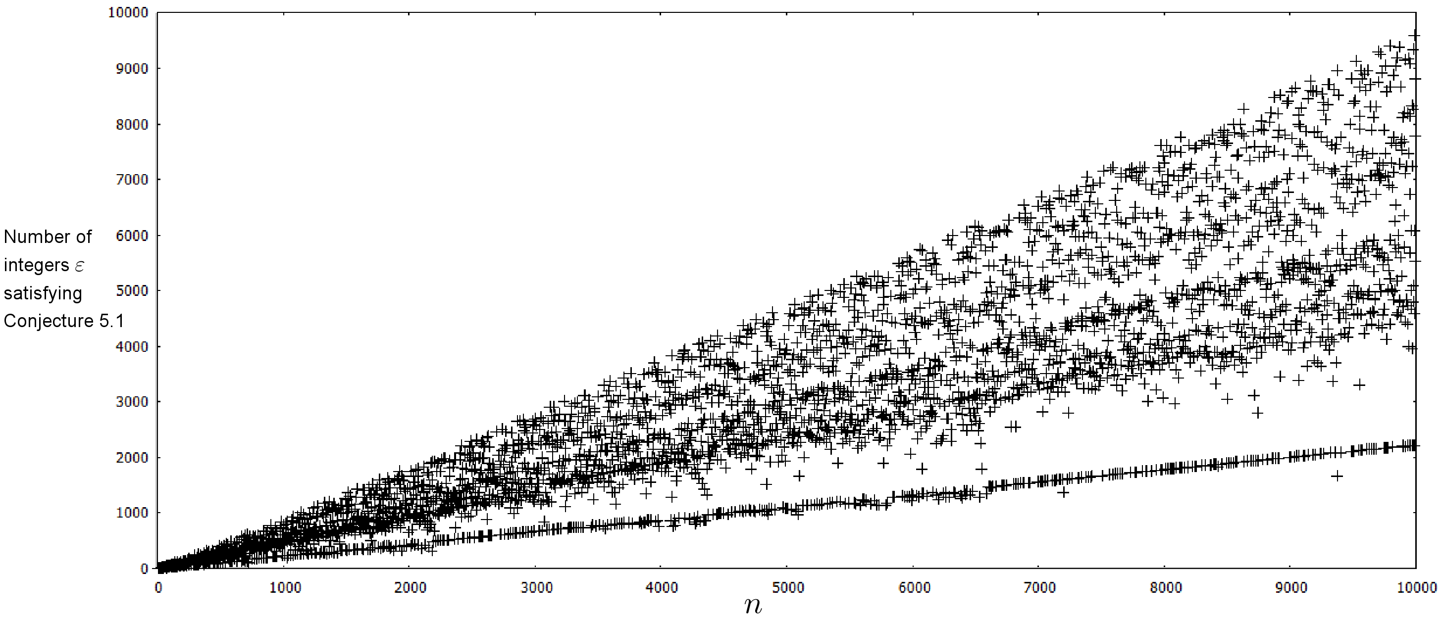
Conjecture 5.1.

Suppose $n$ is even and $n+1$ is not a prime power. Then there exists an integer $\varepsilon\in\left\{2,\ldots,n-1\right\}$ such that $\gcd\left(R_{n}\left(\varepsilon\right),n+1\right)=1$ .

Suppose this conjecture is true. Given a complex even dimension $n$ such that $n+1$ is not a prime power, choose $\varepsilon$ to satisfy the conjecture. Choose an integer $b$ to represent the inverse of $R_{n}\left(\varepsilon\right)$ in $\mathbb{Z}_{n+1}^{\times}$ , and choose the sign of $b$ so that $bR_{n}\left(\varepsilon\right)>0$ . Then by Proposition 2.12, $s_{n}\left[Y_{n}^{\varepsilon}\left(1,b\right)\right]=bR_{n}\left(\varepsilon\right)\equiv 1\mbox{ mod }n+1$ . By Proposition 2.13, each blow-up at a torus-fixed point in this dimension decreases the Milnor genus by $n+1$ . Applying a sequence of such blow-ups to $Y_{n}^{\varepsilon}\left(1,b\right)$ will eventually produce a smooth projective toric variety with Milnor genus equal to one. By (1), this variety can be chosen to represent the cobordism polynomial ring generator $\alpha_{n}$ .

A simple computer program can be used to verify this conjecture in relatively low dimensions.

Proposition 5.2.

Suppose $n$ is even and $n+1$ is not a prime power. If $n\leq 100\,000$ then there exists an integer $\varepsilon\in\left\{2,\ldots,n-1\right\}$ such that $\gcd\left(R_{n}\left(\varepsilon\right),n+1\right)=1$ .

Remark 5.3.

If $n\neq 20$ and $n\neq 50$ , then an $\varepsilon$ that is prime and greater than the largest prime factor of $n+1$ can be chosen to satisfy Proposition 5.2. For $n=20$ and $n=50$ , we can choose $\varepsilon=7$ and $\varepsilon=21$ , respectively. A much faster and more efficient computer program can be used to verify Conjecture 5.1 in the remaining dimensions $n\leq 100\,000$ by only checking prime numbers for $\varepsilon$ .

Corollary 5.4.

If $n\leq 100\,001$ , then there exists a smooth projective toric variety whose cobordism class can be chosen for the polynomial generator $\alpha_{n}$ of $\Omega_{*}^{U}\cong\mathbb{Z}\left[\alpha_{1},\alpha_{2},\ldots\right]$ .

Not only is there an integer $\varepsilon$ satisfying Conjecture 5.1 in dimensions $n\leq 100\,000$ , but the number of such $\varepsilon$ seems to increase in general as $n$ increases. Figure 2 displays this trend. It shows the number of $\varepsilon$ satisfying Conjecture 5.1 for each even $n\leq 10\,000$ such that $n+1$ is not a prime power. In order to verify the conjecture, only one such $\varepsilon$ needs to exist for any given $n$ . It seems likely that the trend in the graph would continue for larger $n$ , making it doubtful that there exists some large complex dimension $n$ for which there is no corresponding $\varepsilon$ that satisfies the conjecture.

6. Conclusion

The evidence supporting Conjecture 5.1 makes it seem very likely that a smooth projective toric variety can be chosen to represent the polynomial generators of the complex cobordism ring in each dimension. Finding a proof of Conjecture 5.1 may be the easiest way to verify this. Unfortunately, the techniques that have been used to prove the existence of smooth projective toric variety polynomial generators still do not result in very convenient choices (see Theorems 3.4 and 4.4 and also Conjecture 5.1).

Remark 3.2 and Figure 2 suggest that there may be many non-cobordant choices for smooth projective toric variety polynomial generators in a given dimension. It therefore seems worthwhile to search for other smooth projective toric varieties for which, like the $Y_{n}^{\varepsilon}\left(a,b\right)$ , the Milnor genus is straight-forward to compute, and there is a large variety of possible values for these Milnor genera. Perhaps this would lead to the discovery of smooth projective toric varieties that can be chosen as polynomial generator representatives that are also easy to describe and work with.

Recall that the varieties $Y_{n}^{\varepsilon}\left(a,b\right)$ consist of a stack of two $\mathbb{C}P^{i}$ -bundles over some $\mathbb{C}P^{k}$ . As an example of the possible diversity of toric polynomial generators, we could instead consider certain smooth projective toric varieties classified by Kleinschmidt that can be viewed as $\mathbb{C}P^{k}$ -bundles over $\mathbb{C}P^{n-k}$ [13]. At the level of fans, these varieties correspond to fans which have exactly two more generating rays than the dimension. These provide additional, often non-cobordant examples of smooth projective toric variety polynomial generators in many dimensions [17, Chapter 5].

There are many other examples of smooth projective toric varieties that may also be useful in finding complex cobordism polynomial generators. For example, Batyrev classified all smooth projective toric varieties corresponding to fans with three more generating rays than the dimension [1]. These display a convenient structure which facilitates computations of Milnor genera. Cayley polytopes (see [7] for details) also display a simple structure which facilitates computing the Milnor genus of the corresponding toric varieties. More refined techniques for computing the Milnor genera of these smooth projective toric varieties could lead to the discovery of convenient and easy to describe complex cobordism polynomial generators among them.

References

[1] Victor V. Batyrev. On the classification of smooth projective toric varieties. Tohoku Mathematical Journal, 43:569–585, 1991.
[2] Victor M. Buchstaber and Taras E. Panov. Torus Actions and Their Applications in Topology and Combinatorics, volume 24 of University Lecture Series. American Mathematical Society, Providence, RI, 2002.
[3] V. M. Buchstaber and N. Ray. Toric manifolds and complex cobordisms. Russian Mathematical Surveys, 53(2):371–373, 1998.
[4] Victor M Buchstaber and Nigel Ray. Tangential structures on toric manifolds, and connected sums of polytopes. International Mathematical Research Notices, 4:193–219, 2001.
[5] David A. Cox, John B. Little, and Henry K. Schenck. Toric Varieties, volume 124 of Graduate Studies in Mathematics. American Mathematical Society, 2011.
[6] V. I. Danilov. The geometry of toric varieties. Russian Mathematical Surveys, 33(2):97–154, 1978.
[7] Alicia Dickenstein, Sandra Di Rocco, and Ragni Piene. Classifying smooth lattice polytopes via toric fibrations. Advances in Mathematics, 222(1):240–254, 2009.
[8] William Fulton. Introduction to Toric Varieties. Number 131 in Annals of Mathematical Studies. Princeton University Press, 1993.
[9] Phillip Griffiths and Joseph Harris. Principles of Algebraic Geometry. Wiley, New York, 1978.
[10] Daniel Huybrechts. Complex Geometry: An Introduction. Springer, 2005.
[11] Bryan Johnston The values of the Milnor genus on smooth projective connected complex varieties. Topology and its Applications, 138:189–206, 2004.
[12] J. Jurkiewicz. Torus embeddings, polyhedra, k*-actions and homology. Dissertationes Mathematicae, 236, 1985.
[13] Peter Kleinschmidt. A classification of toric varieties with few generators. Aequationes Mathematicae, 35:254–266, 1988.
[14] S. P. Novikov. Some problems in the topology of manifolds connected with the theory of Thom spaces. Doklady Akademii Nauk SSSR, 132(5):1031–1034, 1960.
[15] Robert E. Stong. Notes on Cobordism Theory. Princeton University Press, 1968.
[16] René Thom. Travaux de Milnor sur le cobordisme. Séminaire Bourbaki, 5(180):169–177, 1995.
[17] Andrew Wilfong. Toric Varieties and Cobordism. PhD thesis, University of Kentucky, 2013.