On the fluid behavior of a baryon rich hadron resonance gas

The main goal of ultrarelativistic heavy ion collisions is to create and study new states of nuclear matter. The Relativistic Heavy Ion Collider (RHIC) and the Large Hadron Collider (LHC) are able to reach collisional energies high enough to create the Quark-Gluon Plasma (QGP) [1], a new state of nuclear matter in which the quarks and gluons are the relevant degrees of freedom [2]. One of the most surprising discoveries made at RHIC and later confirmed at the LHC is that the QGP seems to behave as a nearly ideal fluid, with one of the smallest values for the shear viscosity to entropy density ratio, $\eta/s$, ever observed in nature [3].

In the last two years, RHIC started to investigate collisions at lower energies, the so-called RHIC low energy scan, in order to probe the phase diagram of nuclear matter at large baryon chemical potentials and to study the existence of a critical point [4]. A striking discovery made by the low energy scan program was that the differential elliptic flow of charged hadrons, $v_{2}(p_{T})$, does not change considerably as one goes to lower collisional energy [5]. This came as a surprise since the large values of $v_{2}(p_{T})$ observed at RHIC’s highest energy were taken as the main evidence for the “almost” ideal fluid nature of the QGP [3]. The fact that such a high differential flow coefficient is also observed at smaller collisional energies, in which the QGP is only present during a very small fraction of the total lifetime of the system, may suggest that the hadron gas formed at the end of the collision can also exhibit strong collective flow. Several calculations [6, 7, 8, 9] based on fluid-dynamical and/or transport models performed at lower RHIC energies have tried to understand how such large differential elliptic flow can occur even at these energies. However, at nonzero baryon chemical potential, the uncertainties in the equation of state and in the transport coefficients, and the existence of baryon stopping in the initial stages render such a task more complicated.

Recently, it was shown that the dissipative effects on $v_{2}(p_{T})$ at RHIC’s top energy originate mostly from the viscosity of the QGP around the (pseudo) phase transition and the viscosity of the hadron gas formed afterwards [10]. As one goes to higher energies, $v_{2}(p_{T})$ becomes more sensitive to the viscosity of the QGP phase (which is expected to increase with temperature), while if one goes to smaller energies, this observable becomes more and more sensitive to the viscosity of the hadron gas (which is expected to increase with decreasing temperature). Since $\eta/s$ increases with decreasing temperature in the hadron gas phase, one would naively expect $v_{2}(p_{T})$ to become considerably smaller as the initial collisional energy of the system is reduced.

Note that the aforementioned behavior of $\eta/s$ as a function of energy was only estimated for nuclear systems at zero baryon chemical potential [11, 12, 13]. Therefore, it is important to understand how this is modified in the presence of a finite baryon chemical potential, $\mu_{B}$. Previous works already indicate that the $\eta/s$ of a gas is reduced at finite chemical potential [14, 15]. For example, $\eta/s$ was computed for a pion-nucleon gas in Ref. [15] using the Chapman-Enskog formalism [16] and it was shown to be reduced when $\mu_{B}>0$. The exception is in Ref. [17], where the $\eta/s$ of a hadron resonance gas was estimated in the excluded volume hadron gas model using a simplified Ansatz for the shear viscosity coefficient. In that work the result obtained was that $\eta/s$ is increased when the baryon chemical potential is nonzero.

On the other hand, it is important to state here that the fluidity of a system at finite chemical potential cannot be inferred by the smallness of $\eta/s$, as was argued in Ref. [18]. A more realistic measure of fluidity would be the ratio of shear viscosity over the enthalpy multiplied by the temperature, $\eta T/(\epsilon+p)$. Note that, when the chemical potential is zero, this quantity reduces to the ratio between shear viscosity and entropy density. On the other hand, when $\mu_{B}$ is large $\eta T/(\epsilon+p)$ considerably differs from $\eta/s$, which can make a difference when analyzing how well a certain system flows (the same can be said for systems that are chemically frozen).

In this work, we compute the shear viscosity of a hadron resonance gas at nonzero temperature and baryon chemical potential using Chapman-Enskog theory [16, 19] within a simple hadronic model [20]. We then compute $\eta T/(\epsilon+p)$ for this system and show that it is considerably reduced when the baryon chemical potential is nonzero. For the values of baryon chemical potential expected to occur around the (chemical freeze-out) phase transition of QCD [21, 22, 23, 24, 25, 26], this reduction is shown to be particularly large. This result suggests that the baryon rich hadron gas formed in the intermediate energies obtained at RHIC, and at future facilities such as FAIR [27], can display strong collective flow, as already implied by the flow harmonic data obtained at RHIC.

In this work the metric tensor is $g^{\mu\nu}\equiv\mathrm{diag}(+,-,-,-)$ and natural units are employed, $\hbar=c=k_{B}=1$. Furthermore, we limit our discussion to Boltzmann gases.

We start by generalizing the method proposed in Ref. [19] to calculate the retarded Green’s function associated with the shear-stress tensor for the case of a dilute multi-component system. As shown in Ref. [19], this formalism will give the same answer as the Chapman-Enskog expansion [16] for the linear coefficients of the Burnett theory [28], i.e., the gradient expansion.

We perform our calculations in the local rest frame of the fluid where $u^{\mu}=(1,0,0,0)$. Since we restrict our discussion to shear viscosity, we may consider the simplified scenario in which the fluid does not accelerate, $u^{\mu}\partial_{\mu}u^{\nu}\equiv 0$, nor expands, $\partial_{\mu}u^{\mu}\equiv 0$, and the temperature, $T=\beta_{0}^{-1}$, and chemical potential, $\mu^{i}=\alpha_{0}^{i}/\beta_{0}$, do not vary in space and time. Here, $\mu^{i}=b_{i}\mu_{B}$, where $\mu_{B}$ is the baryon chemical potential and $b_{i}$ is the baryon number of the $i$–th hadron species. For the sake of simplicity, we only consider classical statistics.

After these simplifications, the Boltzmann equation linearized around a classical equilibrium state, $f_{0\mathbf{p}}^{\left(i\right)}=\exp(\alpha_{0}^{i}-\beta_{0}E_{\mathbf{k}i})$, becomes [19]

where $E_{\mathbf{k}i}$ is the energy of the particle, $N_{\mathrm{spec}}$ is the number of hadron species considered, $\nabla_{\mu}=\Delta_{\mu}^{\nu}\partial_{\nu}$ is the spatial derivative, and $\sigma_{\mu\nu}=\nabla_{\left\langle\mu\right.}u_{\left.\nu\right\rangle}$ is the shear tensor. We defined $\Delta_{\nu}^{\mu}\equiv g_{\nu}^{\mu}-u^{\mu}u_{\nu}$, $\mathbf{v}_{i}\equiv\mathbf{k/}E_{\mathbf{k}i}$, $\delta f_{\mathbf{k}}^{\left(i\right)}\equiv f_{\mathbf{k}}^{\left(i\right)}-f_{0\mathbf{k}}^{\left(i\right)}$, and $A^{\left\langle\mu\nu\right\rangle}=\Delta^{\mu\nu\alpha\beta}A_{\alpha\beta}$ where $\Delta^{\mu\nu\alpha\beta}=\left(\Delta^{\mu\alpha}\Delta^{\nu\beta}+\Delta^{\mu\beta}\Delta^{\nu\alpha}\right)/2-\Delta^{\mu\nu}\Delta^{\alpha\beta}/3$ is the doubly symmetric, traceless projection operator. Also, we introduced the linearized collision operator, $\hat{C}_{ij}$,

Here, $dK_{i}\equiv g_{i}d^{3}\vec{k}/\left[(2\pi)^{3}k_{i}^{0}\right]$ is the Lorentz-invariant measure, $g_{i}$ is the degeneracy factor of the $i$–th hadron species, $\gamma_{ij}=1-\left(1/2\right)\delta_{ij}$, and $g_{i}g_{j}W_{\mathbf{kk}\prime\rightarrow\mathbf{pp}\prime}^{ij}=s\sigma_{ij}\left(2\pi\right)^{6}\delta^{4}\left(p_{i}+p_{j}^{\prime}-k_{i}-k_{j}^{\prime}\right)$ is the corresponding transition rate, with $\sigma_{ij}$ being the differential cross section and $s$ the Mandelstan variable.

Using Eqs. (1) and (2), we express the Fourier transform of the shear-stress tensor, $\tilde{\pi}^{\mu\nu}(Q)$, in terms of the Fourier transform of the shear tensor, $\tilde{\sigma}_{\alpha\beta}(Q)$, in the traditional form of linear response $\tilde{\pi}^{\mu\nu}=G_{R}^{\mu\nu\alpha\beta}\tilde{\sigma}_{\alpha\beta}$ [19]. The Green’s function has the following structure

where $Q^{\mu}=(\omega,\mathbf{q})$ and we used the definition of the total shear-stress tensor of a multi-component system

Our goal is to compute the above retarded Green’s function and its derivatives at vanishing wavenumber. This will be enough to determine the relevant transport coefficients of linearized relativistic fluid dynamics. Following the strategy outlined in [19], we start by introducing the irreducible second rank tensor $B^{\alpha\beta}\left(Q,K_{i}\right)$, which satisfies the following integro-differential equation,

In general, $B^{\alpha\beta}$ is a function of $Q$ but, as mentioned above, we shall only need it at vanishing wavenumber, $\mathbf{q}=0$. Then $B^{\alpha\beta}=B^{\alpha\beta}\left(\omega,K_{i}\right)$ and its dependence on $k_{i}^{\mu}$ can be described by the following expansion,

Substituting Eq. (6) into Eq. (3), it follows that

where we used [20]

Then, the linear relation between $\pi^{\mu\nu}$ and $\sigma^{\mu\nu}$ can be cast into a more convenient form, $\tilde{\pi}^{\mu\nu}\left(\omega,\mathbf{0}\right)=2\tilde{G}_{R}\left(\omega,\mathbf{0}\right)\tilde{\sigma}^{\mu\nu}\left(\omega,\mathbf{0}\right)$, where we introduced the retarded Green’s function

Equations such as (5) appear quite often in problems involving the extraction of transport coefficients from the Boltzmann equation. The way to solve this equation is to substitute the expansion (6) into Eq. (5), multiply by the basis component chosen to expand $B^{\alpha\beta}$, i.e., multiply by $E_{i\mathbf{k}}^{m}k_{i}^{\left\langle\mu\right.}k_{i}^{\left.\nu\right\rangle}$, and integrate over $dK_{i}$. Then one obtains

The function $a_{n}\left(\omega\right)$ can be solved by inverting the above equation.

For any practical calculation, however, only a finite number of basis elements are used in the expansion of $B^{\alpha\beta}$. Truncating such momentum expansion is a common approach in kinetic theory and happens, for example, when dealing with the Chapmann-Enskog expansion [16]. Here we use the simplest truncation possible in which only one member of the basis is used (this is equivalent to the 14-moment approximation in the method of moments [19, 29, 30]). This truncation should still provide transport coefficients that are accurate up to $\sim 10\%$ (see, for instance, Refs. [20, 31]). In such simplified approximation,

where

The formal solution for $a_{0}^{\left(i\right)}\left(\omega\right)$ is

where $\mathbf{\hat{C}}^{ij}=\mathcal{C}^{\left(ij\right)}$, and the retarded Green’s function, $\tilde{G}_{R}\left(\omega,\mathbf{0}\right)$, becomes

The derivative of this Green’s function at zero frequency is

The linearized Burnett equation emerging from the above Green’s function is

where the shear viscosity coefficient is identified as

and the transport coefficient of the second order term $2\Delta_{\alpha\beta}^{\mu\nu}u^{\lambda}\partial_{\lambda}\sigma^{\alpha\beta}$, here referred to as $\lambda$, is given by

Nonlinear terms that may be included in the gradient expansion are not considered in this work.

In the following, we briefly discuss how thermodynamic quantities are computed in a multi-component gas. The baryon number density, $n_{B}$, the energy density, $\varepsilon$, and the thermodynamic pressure, $P$, are computed using the hadron resonance gas model,

The entropy density, $s$, is computed using the following thermodynamic relation

The enthalpy, $h$, is defined as

Note that the ratio of enthalpy to temperature is equivalent to the entropy density when the baryon chemical potential is zero, i.e., when $\mu_{B}=0$, $h=Ts$ .

In Fig. 1 we show the entropy density and the ratio of enthalpy to temperature as a function of temperature for $\mu_{B}=0$ and $\mu_{B}=0.5$ GeV. It is clear that both these thermodynamic quantities increase in the presence of a positive baryon chemical potential, with the increase in $h/T$ being more pronounced.

The purpose of this work is not to compute the transport properties of a hadron gas with precision. In order to accomplish this, one would have to know the cross sections of all processes involving the known hadrons and resonances as well as include the effect of Hagedorn states and repulsive interactions. Currently, the inclusion of all these effects with precision is just not possible. What we actually aim to investigate is how the fluidity of such a gas is modified when the baryon chemical potential is present. This effect can be consistently estimated with a more simple model of a hadron gas in which all cross sections are constant and fixed to a certain value. Here, we shall consider two cases: (i) assume that all hadrons have a $1$ fm radius, leading to total cross-sections of $\sigma_{T}=\pi$ fm² and (ii) assume that meson-meson, meson-baryon, and baryon-baryon cross sections scale as $4:6:9$, respectively, with the baryon-baryon cross section beying set to $\pi$ fm². That is, in case (ii) $\sigma_{\mathrm{meson-meson}}=4/9\times\sigma_{\mathrm{baryon-baryon}}$ and $\sigma_{\mathrm{meson-baryon}}=2/3\times\sigma_{\mathrm{baryon-baryon}}$. Such simplified systems can be used to estimate the effects of a nonzero baryon chemical potential on the transport coefficients of a hadron resonance gas. For constant cross-sections, it is straightforward to solve integrals (12) and (13). Then, $\eta$ and $\lambda$ can be computed from Eqs. (16) and (17), while all thermodynamic quantities are computed from the formulas specified in the previous section.

In the following, we shall consider $3$ different choices of baryon chemical potential: $\mu_{B}=0$, $\mu_{B}=500$ MeV, and the $\mu_{B}(T)$ obtained from thermal fits to heavy ion collisions at several collisional energies. In Ref. [25], the following parametrization of $T\left(\mu_{B}\right)$ was extracted from thermal fit calculations,

where $a\simeq 0.166$ GeV, $b\simeq 0.139$ GeV^-1, and $c\simeq 0.053$ GeV^-3. This parametrization provides the temperature as a function of baryon chemical potential in the chemical freeze-out transition. In practice, the chemical freeze-out transition is very close to the actual (pseudo) phase transition region and we will use this parametrization to estimate $T\left(\mu_{B}\right)$ near the phase transition region. Here, we just invert Eq. (19) to obtain $\mu_{B}\left(T\right)$. Finally, we consider all hadrons and resonances with masses up to $2$ GeV, where the masses and degeneracy factors of each hadron/resonance are taken from Ref. [32].

In Fig. 2 we show $\eta/s$ (left panel) and $\eta T/h$ (right panel) as function of $T$ for the $3$ baryon chemical potential choices described above and for the cross section of case (i). The black dotted line corresponds to $\mu_{B}=0$, the red dash-dotted line corresponds to $\mu_{B}=500$ MeV, and the blue solid line corresponds to $\mu_{B}(T)$ from Ref. [25].

One can see that a finite baryon chemical potential can have a very large effect on $\eta/s$. The effect is particularly large at the chemical freeze-out transition where $\eta/s$ is reduced by a factor $\sim 3$ at $100$ MeV. As discussed in Ref. [18] and in the Introduction of this paper, at nonzero baryon chemical potential $\eta/s$ is not the correct quantity to estimate the fluidity of the system. In this case, the ratio $\eta T/h$ can provide a better estimate. We see the effect of $\mu_{B}$ is amplified in this case, serving to reduce even more $\eta T/h$. For the case of $\mu_{B}(T)$ defined using the chemical freeze-out transition, we see that $\eta T/h$ is almost constant in temperature, which indicates that the fluid behavior of a hadron resonance gas does not change much in the phase transition region. This suggests that the systems created in the RHIC low energy runs can exhibit substantial elliptic flow since $v_{2}(p_{T})$ should be dominated by the shear viscosity near the phase transition [10].

We remark that this dependence of $\eta/s$ (or $\eta T/h$) on $\mu_{B}$ originates mostly from the thermodynamic variables, e.g. $s$ and $h/T$. The shear viscosity coefficient itself increases with $\mu_{B}$, even though this effect is small. The reduction of $\eta/s$ and $\eta T/h$ with $\mu_{B}$ happens mostly because $s$ and $h/T$ increase by a significant amount when $\mu_{B}$ is present and is of the order $\mu_{B}\sim 500$ MeV. In the Ref. [17], the increase of $\eta/s$ with $\mu_{B}$ must have been due to the excluded volume effect. We note, however, that in the equation of state usually employed in heavy ion collision simulations (and that describes reasonably well lattice QCD simulations) the excluded volume correction is not included, for details see Ref. [33].

In Fig. 3 we show $\eta/s$ (left panel) and $\eta T/h$ (right panel) as function of $T$ for the $3$ baryon chemical potential choices described above and for the cross section of case (ii). The results are qualitatively similar to those found in case (i). The main difference is that $\eta/s$ and $\eta T/h$ decrease faster with increasing temperature for cross sections (ii) since the meson-meson cross section is almost a factor two smaller than the baryon-baryon cross section and, at low temperatures $\sim 100$ MeV, the system is dominated by mesons (mostly pions). This can be seen by comparing Figs. 2 and 3. One should note that, in the hadron resonance gas model, the thermodynamic quantities are independent of the cross sections and, consequently, the entropy density, energy density, and thermodynamic pressure do not change going from case (i) to case (ii).

It is also useful to see what happens to the transport coefficients of terms that are of second order in gradients. In Fig. 4, we show the transport coefficient $\lambda$, that multiplies the next order (linear) term in the Burnett equation (i.e., the gradient expansion), for cases (i) (left panel) and (ii) (right panel). In this case, this is the coefficient that multiplies the term $\dot{\sigma}^{\mu\nu}$. We plot the following dimensionless combination $\lambda T/\eta$ in Fig. 4 and one can see that this dimensionless ratio is also reduced when baryon chemical potential is present. From a qualitative perspective, the effect is very similar to what happens to $\eta T/h$. The result is qualitatively the same for both choices of cross sections.

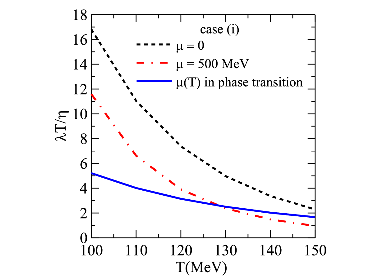
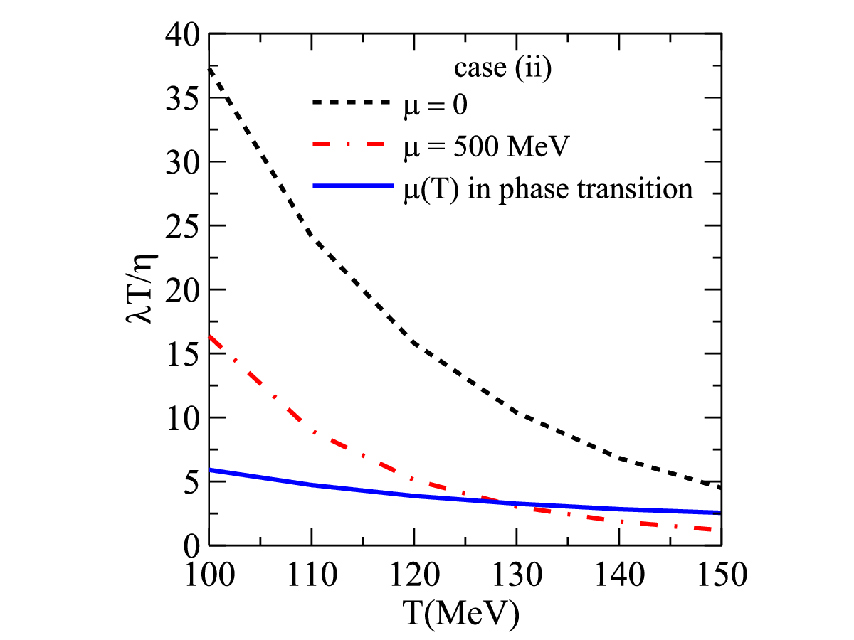
This shows that the fluidity of a baryon rich hadron gas is in fact larger than the equivalent system at vanishing baryon number. Not only $\eta T/\left(\varepsilon+p\right)$ is considerably smaller, but the dimensionless combination $\lambda T/\eta$, associated with a term of second order in gradients of velocity, becomes considerably smaller when $\mu_{B}$ is nonzero.

In this paper we investigated the effects of a nonzero baryon chemical potential on the transport properties of a hadron resonance gas. We found that a hadron resonance gas with large baryon number density is closer to the ideal fluid limit than the corresponding gas with zero baryon number. A nonzero baryon chemical potential served not only to reduce the effect of dissipative terms of first order in gradients but also of terms that are of second order. This suggests that the system created at RHIC at lower collision energies may display a fluid-like behavior with an effective fluidity close to the one found at RHIC’s highest energy collisions. This may explain why the differential elliptic flow coefficient measured at lower collisional energies at RHIC is close to the one measured at high energies.

G. S. Denicol, S. Jeon, and C. Gale acknowledge support by the Natural Sciences and Engineering Research Council of Canada. J. Noronha thanks Fundação de Amparo à Pesquisa do Estado de São Paulo (FAPESP) and Conselho Nacional de Desenvolvimento Científico e Tecnológico (CNPq) for support.

References

- [1] D. H. Rischke, Prog. Part. Nucl. Phys. 52, 197 (2004).
- [2] BRAHMS collaboration, Nuclear Physics A 757, Issues 1-2, Pages 1-27 (2005); PHENIX collaboration, Nuclear Physics A 757, Issues 1-2,Pages 184-283 (2005); PHOBOS collaboration, Nuclear Physics A 757, Issues 1-2, Pages 28-101 (2005); STAR collaboration, Nuclear Physics A 757, Issues 1-2, Pages 102-183 (2005).
- [3] M. Gyulassy and L. McLerran, Nucl. Phys. A 750, 30 (2005).
- [4] M. A. Stephanov, K. Rajagopal and E. V. Shuryak, Phys. Rev. Lett. 81, 4816 (1998); Phys. Rev. D 60, 114028 (1999).
- [5] L. Adamczyk et al. [STAR Collaboration], Phys. Rev. C 86, 054908 (2012).
- [6] C. Shen and U. Heinz, Phys. Rev. C 85, 054902 (2012) [Erratum-ibid. C 86, 049903 (2012)].
- [7] J. Auvinen and H. Petersen, arXiv:1306.0106 [nucl-th].
- [8] S. Plumari, V. Greco and L. P. Csernai, arXiv:1304.6566 [nucl-th].
- [9] D. Solanki, P. Sorensen, S. Basu, R. Raniwala and T. K. Nayak, Phys. Lett. B 720, 352 (2013).
- [10] H. Niemi, G. S. Denicol, P. Huovinen, E. Molnar and D. H. Rischke, Phys. Rev. Lett. 106, 212302 (2011); H. Niemi, G. S. Denicol, P. Huovinen, E. Molnar and D. H. Rischke, Phys. Rev. C 68, 014909 (2012)
- [11] M. Prakash, M. Prakash, R. Venugopalan and G. Welke, Phys. Rept. 227, 321 (1993).
- [12] J. Noronha-Hostler, J. Noronha and C. Greiner, Phys. Rev. Lett. 103, 172302 (2009); J. Noronha-Hostler, J. Noronha and C. Greiner, Phys. Rev. C 86, 024913 (2012).
- [13] A. Wiranata and M. Prakash, Phys. Rev. C 85, 054908 (2012); A. Wiranata, V. Koch, M. Prakash and X. N. Wang, arXiv:1307.4681 [hep-ph].
- [14] N. Demir and S. A. Bass, Phys. Rev. Lett. 102, 172302 (2009).
- [15] K. Itakura, O. Morimatsu and H. Otomo, Phys. Rev. D 77, 014014 (2008).
- [16] S. Chapman and T. G. Cowling, The Mathematical Theory of Non-Uniform Gases, (3rd ed., Cambridge University Press, New York A974);
- [17] M. I. Gorenstein, M. Hauer and O. N. Moroz, Phys. Rev. C 77, 024911 (2008).
- [18] J. Liao and V. Koch, Phys. Rev. C 81, 014902 (2010).
- [19] G. S. Denicol, J. Noronha, H. Niemi and D. H. Rischke, Phys. Rev. D 83, 074019 (2011); G. S. Denicol, J. Noronha, H. Niemi and D. H. Rischke, J. Phys. G 38, 124177 (2011).
- [20] S. R. de Groot, W. A. van Leeuwen, and Ch. G. van Weert, Relativistic kinetic theory - Principles and applications, (North-Holland, 1980).
- [21] A. Andronic, P. Braun-Munzinger and J. Stachel, Phys. Lett. B 673, 142 (2009) [Erratum-ibid. B 678, 516 (2009)].
- [22] A. Andronic, P. Braun-Munzinger and J. Stachel, Nucl. Phys. A 772, 167 (2006).
- [23] J. Cleymans and K. Redlich, Phys. Rev. Lett. 81, 5284 (1998).
- [24] J. Cleymans and K. Redlich, Phys. Rev. C 60, 054908 (1999).
- [25] J. Cleymans, H. Oeschler, K. Redlich and S. Wheaton, Phys. Rev. C 73, 034905 (2006).
- [26] J. Noronha-Hostler, H. Ahmad, J. Noronha and C. Greiner, Phys. Rev. C 82, 024913 (2010).
- [27] See, for instance, the website http://www.fair-center.eu/.
- [28] D. Burnett, Proc. Lond. Math. Soc. 39, 385 (1935); Proc. Lond. Math. Soc. 40, 382 (1936).
- [29] W. Israel and J. M. Stewart, Ann. Phys. (N.Y.) 118, 341 (1979).
- [30] G. S. Denicol, T. Koide and D. H. Rischke, Phys. Rev. Lett. 105, 162501 (2010).
- [31] G. S. Denicol, H. Niemi, E. Molnar and D. H. Rischke, Phys. Rev. D 85, 114047 (2012).
- [32] J. Beringer et al. (Particle Data Group), Phys. Rev. D 86, 010001 (2012).
- [33] P. Huovinen and P. Petreczky, Nucl. Phys. A 837, 26 (2010).