Percolation of Interdependent Networks with Inter-similarity

Single isolated networks have been extensively studied in the past decade [2, 3, 4, 5, 6, 7, 8, 9, 10, 11, 12, 13, 14, 15, 16]. Recently, much interest has been devoted to interdependent networks [17, 18, 19, 20, 21, 22, 23, 24, 25, 26, 27, 28], which can model some real world catastrophic events, such as the electrical blackout in Italy on Sep. 28th, 2003 [29] and the US-Canada Power system outage on Aug. 14th, 2003 [30]. Failures of a small number of power stations can cause further malfunction of nodes in their communication control network, which in turn leads to the shutdown of power stations [17, 29]. This cascading process continues until no more nodes fail due to percolation or due to interdependence failures. In contrast to single networks where the percolation transition is continuous, in interdependent networks the transition is abrupt [17, 18].

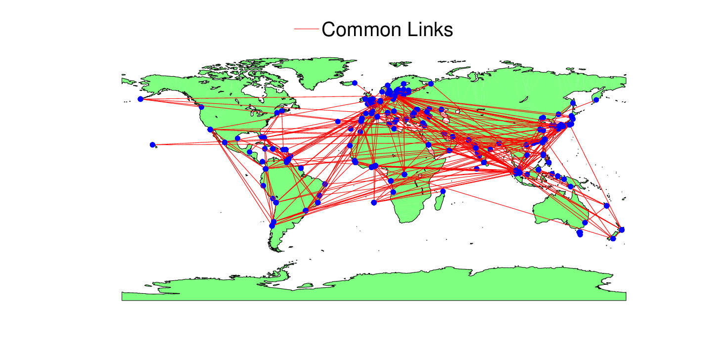
Real interdependent networks are sometimes coupled according to some inter-similarity features. Intersimilarity means the tendency of neighboring nodes in one network to be interdependent of neighboring nodes in the other network. Such coupled networks, are more robust against cascading failures than randomly coupled interdependent networks. To quantify self-similarity, Parshani et al. introduced the inter-clustering coefficient (ICC), which measures the average number of common links per pair of interdependent nodes [1]. Common links are defined as follows: Given two coupled networks $A$ and $B$, and two nodes $a_{k}$ and $a_{l}$ which are linked in $A$. If their interdependent counterparts $b_{k}$ (corresponds to $a_{k}$) and $b_{l}$ (corresponds to $a_{l}$) in $B$ are also linked (in $B$), this pair of links is called a common link. Common links can be interpreted as follows, if two nodes in one network are linked, the tendency (probability) of their interdependent counterparts in the other network to be linked is a measure of the inter-similarity. Thus, the density of the common links reflects the inter-similarity of the two networks. In the extreme case where every pair of links is a common link, the two networks are identical. In this case no cascading failure will occur, since a failure in network A will cause an identical failure in B and there will be no cascading failure feedback to A. It is therefore expected that the more common links appear in the coupled networks system, it becomes more robust. In the example of the coupled world wide port network and the airline network, illustrated in Fig. 1, the fraction of common links is 0.12 for the port network and 0.18 for the airline network [1]. Therefore, developing a method to analyze cases where certain common topologies exist in the interdependent networks can help to understand the vulnerabilities of coupled complex systems in real world as well as for designing robust infrastructures.

In this paper, we introduce a method to analytically calculate the cascading process of failures in interdependent networks with common links. To analyze this problem, we consider the cluster components of the network composed of only common links after the initial attack. We will illustrate that all nodes in such a component will survive or fail simultaneously during the cascading process. Based on this fundamental feature, we divide the system into subnetworks according to the sizes of the components, and then contract all nodes in each component into a single node. After contraction, the system degenerates into two randomly coupled networks without common links, which will be solved analytically. Here, we find the exact solution for the case where $A$ and $B$ are fully interdependent Erdős-Rényi (ER) networks each of average degree k and the network of common links is also an ER network with the average degree $K$. In this case, we show that the interdependent networks system undergoes a first order transition for all $K\geq 0$.

The paper is organized as follows. In Sec. II, we introduce the model of cascading failures in interdependent networks with common links. In Sec. III, we analyze the process of failures and the final state where the process ends. In Sec. IV, we derive our theoretical results and compare them with simulation results.

For simplicity and without loss of generality we analyze the percolation process in a system of two fully interdependent networks $A$ and $B$ of the same size $N$ with no-feedback condition [23] in the presence of common links. The no-feedback means that, each $A$-node $a_{k}$ has one and only one dependency counterpart $b_{k}$ on network $B$, and $b_{k}$ must depend only on $a_{k}$. Initially, a fraction $1-p$ of $A$ nodes are removed randomly. Due to interdependency, a corresponding fraction of $B$-nodes also fail. We denote by $A_{0}$ and $B_{0}$ the remaining networks of size $N_{0}=pN$. Nodes of $A_{0}$ and $B_{0}$ are represented by $a_{i}$ and $b_{i}$ respectively, $i=1,...,N_{0}$, and $a_{i}$ interdepends on $b_{i}$ for all $i=1,2,...,N$. The pair $(i,j)$ is a common link if $a_{i}$ is linked to $a_{j}$ and $b_{i}$ is also linked to $b_{j}$. We introduce a network $C_{0}$ that includes all $N_{0}$ nodes but only links that are common links. This means that the nodes $c_{i}$ and $c_{j}$ of $C_{0}$ will be linked if and only if both $a_{i},a_{j}$ and $b_{i},b_{j}$ are linked. Analogously, we define a network $C$ which is the collection of common links in the original networks $A$ and $B$. Thus network $C$ reduces to $C_{0}$ due to the initial attack. As shown in Fig.  2, we denote $A_{0}^{\prime}$ and $B_{0}^{\prime}$ to be the networks that composed of the same $N_{0}$ nodes in $A_{0}$ and $B_{0}$ but only those links which are not common links. Therefore, networks $A_{0}$ and $B_{0}$ can be written as matrix summations

We will investigate the robustness of such a system after the initial attack. Notice that when $C_{0}$ has no links since there is no common links in this system. This is the case of random coupling studied by Buldyrev et al [17], since the probability to have a common link in random coupling approach to zero for large N. We will provide a method for analyzing the case when network $C_{0}$ has a given topological structure. Let $R_{0}(m),m=1,2,\cdots,M$ be the component size distribution of $C_{0}$. That is to say, if we randomly choose a node in network $C_{0}$, the probability that it belongs to a component of size $m$ in network $C_{0}$ is $R_{0}(m)$. This distribution is a characterization of both the degree and the structure of inter-similarity of the network.

The initial attack leads to failures of some other nodes in $A_{0}$ since those nodes will lose connectivity with the giant component $A_{1}$ of $A_{0}$ (a percolation failure). Consequently, in $B_{0}$, all nodes that depend on those nodes that have been removed in $A_{0}$ will fail due to interdependency relations (a dependency failure). We use $B_{1}$ to denote the remaining nodes in $B_{0}$. Then, similarly, a percolation failure will occur in $B_{1}$. This will induce an iterative process of percolation failures and dependency failures in the system [31]. Finally, if no further failure occurs, this cascading process will end with a total collapse or two remaining giant components of the same size. We are interested here in the relationship between $p$ and the size of the final mutual giant component.

Notice that during the cascading process, if a node in a component of $C_{0}$ survives, the whole component will survive, and if a node in a component fails, the whole component will fail. Inspired by this basic fact, as shown in Fig. 3, we divide networks $A_{0}$ and $B_{0}$ respectively according to the component sizes in network $C_{0}$. That is to say, in network $A_{0}$, all those nodes that belong to components of size $m=1,2,\cdots,M$ in $C_{0}$ compose a subnetwork denoted by $A_{0}^{(m)}$. Here, $M$ is the largest component size of network $C_{0}$. Network $B_{0}$ can be divided into $B_{0}^{(m)}$, analogously. In this way, the size of each subnetwork $A_{0}^{(m)}$ or $B_{0}^{(m)}$ is $N_{0}^{(m)}=R_{0}(m)N_{0}$, where $m=1,2,\cdots,M$.

As depicted in Fig.  3, we also contract $A_{0}$ and $B_{0}$ according to the components of network $C_{0}$. In other words, in network $A_{0}$, all $m$-nodes that belong to each component of size $m$ in $C_{0}$ are merged into a single new node, and all links connected to at least one of these $m$ nodes are also merged on the new node. All of these merged nodes and links form a contracted network $A^{\prime}_{0}$ with subnetworks $A^{\prime(m)}_{0},m=1,2,\cdots,M$. Network $B_{0}$ is contracted similarly. In this way, the size of each subnetwork $A^{\prime(m)}_{0}$ or $B^{\prime(m)}_{0}$ is just the number of components of size $m$ in network $C_{0}$, that is $N^{\prime(m)}_{0}=\frac{R_{0}(m)N_{0}}{m},m=1,2,\cdots,M$. And the size of $A^{\prime}_{0}$ or $B^{\prime}_{0}$ is $N^{\prime}_{0}=\sum\limits_{m=1}^{M}N^{(m)}_{0}=\sum\limits_{m=1}^{M}\frac{R_{0}(m)N_{0}}{m}=N_{0}\cdot\sum\limits_{m=1}^{M}\frac{R_{0}(m)}{m}$. We denote $\langle m\rangle=\left(\sum\limits_{m=1}^{M}\frac{R_{0}(m)}{m}\right)^{-1}$ as the average component size in $C_{0}$. Thus, we have $N^{\prime}_{0}=\frac{N_{0}}{\langle m\rangle}$.

As shown in Fig. 3(c), common links do not exist any more in the contracted system, because each common link always lies inside a component of network $C_{0}$. In fact, after the initial attack, the cascading process in the contracted system is equivalent to the cascading on the original system. Therefore, we only need to focus on the cascade process in the contracted system.

Here, we exhibit, step-by-step, the theoretical analysis for the cascading process starting from $A^{\prime}_{0}$ and $B^{\prime}_{0}$. In the first stage, the size of the remaining functional giant component $A^{\prime}_{1}$ can be obtained using the method proposed by Leicht and D’Souza [32]. We regard $A^{\prime}_{0}$ as a system of $M$ coupled subnetworks $A^{\prime(m)}_{0}$, $m=1,2,\cdots,M$. If the degree distribution $p^{mm^{\prime}}_{A^{\prime}_{0}}$ ($mm^{\prime}$-degrees) from a randomly chosen node in $A^{\prime(m)}_{0}$ to all nodes in $A^{\prime(m^{\prime})}_{0}$ can be exactly evaluated, then the whole system can be described using multi-variable generating functions. Usually, we analyze the cascading process by three steps to obtain the recursive system [17] .

We use $g^{(m)}_{A^{\prime}_{0}}(p_{1},p_{2},\cdots,p_{M})$ to denote the fraction of nodes in the giant component of $A^{\prime(m)}_{0}$ after randomly removing a fraction $1-p_{m^{\prime}}$ of nodes in each subnetwork $A^{\prime(m^{\prime})}_{0}$, $m^{\prime}=1,2,\cdots,M$. Here, we contract the two coupled networks after the initial attacking. It implies that $p_{m^{\prime}}=0$ at the beginning of the cascading process on the contracted two coupled networks. Thus, the remaining functional part in each subnetwork is $\psi^{(m)}_{1}=g^{(m)}_{A^{\prime}_{0}}(1,1,\cdots,1)$ in the first stage.

The second stage [17] is equivalent to randomly attacking a fraction $1-\psi^{(m)}_{1}$ of nodes in each subnetwork $B^{\prime(m)}_{0}$, $m=1,2,\cdots,M$. We let $\phi^{\prime(m)}_{1}=\psi^{(m)}_{1}$. Therefore, the remaining giant component of $B^{\prime}_{0}$ is $\phi^{(m)}_{1}=\phi^{\prime(m)}_{1}\cdot g^{(m)}_{B^{\prime}_{0}}(\phi^{\prime(1)}_{1},\phi^{\prime(2)}_{1},\cdots,\phi^{\prime(M)}_{1})$.

The third stage is equivalent to randomly removing a fraction $1-g^{(m)}_{B^{\prime}_{0}}(\phi^{(1)}_{1},\phi^{(2)}_{1},\cdots,\phi^{(M)}_{1})$ of nodes in $A^{\prime(m)}_{0}$. We let $\psi^{\prime(m)}_{2}=g^{(m)}_{B^{\prime}_{0}}\cdot(\phi^{(1)}_{1},\phi^{(2)}_{1},\cdots,\phi^{(M)}_{1})$, $m=1,2,\cdots,M$. Thus, the remaining fraction in $A^{\prime}_{0}$ is $\psi^{(m)}_{2}=\psi^{\prime(m)}_{2}\cdot g^{(m)}_{A^{\prime}_{0}}(\psi^{\prime(1)}_{2},\psi^{\prime(2)}_{2},\cdots,\psi^{\prime(M)}_{2})$.

Generally, we have $\psi^{\prime(m)}_{n}=g^{(m)}_{B^{\prime}_{0}}\cdot(\phi^{\prime(1)}_{n-1},\phi^{\prime(2)}_{n-1},\cdots,\phi^{\prime(M)}_{n-1})$, and $\psi^{(m)}_{n}=\psi^{\prime(m)}_{n}\cdot g^{(m)}_{A^{\prime}_{0}}(\psi^{\prime(1)}_{n},\psi^{\prime(2)}_{n},\cdots,\psi^{\prime(M)}_{n})$; $\phi^{\prime(m)}_{n}=g^{(m)}_{A^{\prime}_{0}}(\psi^{\prime(1)}_{n},\psi^{\prime(2)}_{n},\cdots,\psi^{\prime(M)}_{n})$, and $\phi^{(m)}_{n}=\phi^{\prime(m)}_{n}\cdot g^{(m)}_{B^{\prime}_{0}}(\phi^{\prime(1)}_{n},\phi^{\prime(2)}_{n},\cdots,\phi^{\prime(M)}_{n})$, $m=1,2,\cdots,M$.

In the final stage, where the process of cascading failures ceases, we have $\psi^{\prime(m)}_{n}=\psi^{\prime(m)}_{n-1}=\phi^{\prime(m)}_{n}=\phi^{\prime(m)}_{n-1}$ for all $m$. Let $x_{m}=\psi^{\prime(m)}_{n}$, and $y_{m}=\phi^{\prime(m)}_{n}$. We arrive a system of $x_{m}$ and $y_{m}$:

This system can be analytically solved using $M$-variant generating functions. Similar to Ref. [32], for a system of $M$ interconnected subnetworks $A^{\prime(m)}_{0}$, we define the generating function for the degree distributions for each subnetwork as

where, $m,m^{\prime}=1,2,\cdots,M.$ For network $B^{\prime}_{0}$, we can define the analogous generating functions and obtain similarly the giant component size.

For simplicity, we assume that all $mm^{\prime}$-degree distributions in $A^{\prime}_{0}$ and $B^{\prime}_{0}$ are Poisson distributions, whose average degrees are $k^{A^{\prime}_{0}}_{mm^{\prime}}$ and $k^{B^{\prime}_{0}}_{mm^{\prime}}$, respectively. For example, if both $\tilde{A}$ and $\tilde{B}$ are Erdős-Rényi (ER) networks with average degrees $a$ and $b$, respectively, and the initial attack on network $A$ is random, then these $mm^{\prime}$-degrees in $A_{0}$ have Poisson distributions for all $m$ and $m^{\prime}$. Then, according to the result in Ref. [32], we have

where, $m=1,2,\cdots,M.$ Similarly, for network $B^{\prime}_{0}$,

where, $m=1,2,\cdots,M$. The system of the final stage can be written as

By solving this system, we can get $\mu^{(m)}_{\infty}=(1-u_{m})(1-v_{m})$, $m=1,2,\cdots\,M$. This is the fraction of the mutual giant component in each subnetwork $A^{\prime(m)}_{0}$ or $B^{\prime(m)}_{0}$. The fraction of the mutual giant component in the original system of $A$ and $B$ is

Notice that in Eq. (14), $u_{m}=u^{m}_{1}$, and $v_{m}=u^{mb/a}_{1}$, $m=1,2,\cdots,M$. Therefore, the system can be simplified to a single equation for $u_{1}$,

One trivial solution of Eq. (16) is $u_{1}=1$. In some cases, other nontrivial solutions exist in the interval $[0,1)$. The smallest solution $u_{1min}$ corresponds to the size of the final mutual giant component ${-\log u_{1min}}/{a}$. Consider $F_{2}(u_{1})=\exp\left(-ap\sum\limits_{m^{\prime}=1}^{M}R_{0}(m^{\prime})(1-u^{m^{\prime}}_{1})(1-u^{m^{\prime}b/a}_{1})\right)$ and $F_{1}(u_{1})=u_{1}$. Then the critical point $u_{1c}$ and $p^{I}_{c}$ is where a nontrivial solution that satisfies: $F_{1}(u_{1c})=F_{2}(u_{1c})$ and $F^{\prime}_{1}(u_{1c})=F^{\prime}_{2}(u_{1c})$ emerges. Note that, all the analysis is done here on the contracted network system after the initial random removal, which means there is no initial attacking on the contracted system. If $M$ is finite, at the solution $u_{1}=1$, we have $F_{1}(1)=F_{2}(1)=1$, but $F^{\prime}_{1}(1)=1\neq F^{\prime}_{2}(1)=0$. This means these two curves cannot be tangent to each other at $u_{1}=1$. Therefore, $u_{1}=1$ cannot be a critical value for a second order transition, and only first order phase transitions at $u_{1c}<1$ occur in systems with a finite $M$.

Here, we further investigate the case where $C$ (network composed of common links) is an ER network with an average degree $K$. After the random initial attack, $C_{0}$ is also an ER network, whose average degree becomes $Kp$. The component size distribution of $C_{0}$ is $R_{0}(m)=\frac{1}{m!}\cdot(mKp)^{m-1}\cdot e^{-mKp},m=1,2,\cdots$. In this case, $M$ should be in principle infinite. However, when we substitute this distribution into Eq. (16), it is appropriate to use a truncation $m=1,2,\cdots,M<\infty$ on the infinite sum, since $R_{0}(m)$ decays exponentially, and the largest cluster of network $C_{0}$ cannot be as large as $O(N)$ when $Kp<1$. This means $p_{c}<1/K$. Therefore, no matter for $K<1$ or $K\geq 1$, we can use Eq. (16) directly to determine $p_{c}$. The theoretical results are in excellent agreement with simulations and are shown in Fig.  4, Fig.  5 and Fig.  6. Also, notice that for $a=b=0$ and $K\geq 1$, the system will behave like a single ER network and will have a second order transition. Surprisingly, our result indicates that for any $a,b>0$, which means the two networks are not identical, the equation describing the system will become Eq. (16), and the transition will become suddenly from second order when $a=b=0$ to first order.

In this paper we provide an exact solution for interdependent networks with common links (representing inter-similarity in the system), which can be found in many real world network systems. We treat the components composed of inter- similar links as a new kind of nodes, and these new nodes form a new mutually interdependent network system with degree correlation, which comes from the correlation between component sizes. In order to deal with this kind of degree correlation, we decompose the new network system into a series of subnetworks according to their component sizes. That is, the new node correspond to the same component size in each of subnetworks respectively. Then we employ a high dimensional generating function to describe this system and obtain the exact percolation equations which can be solved numerically. If the two mutually interdependent networks are fully inter-similar or identical ($a=b=0$), we know that the percolation is exactly the same with that on a single network and must be a second order phase transition. From the above analysis, we surprisingly find that when the two mutually interdependent networks are not identical ($a,b>0$), the transition is totally different from single networks and is always of first order.

We thanks Prof. Yiming Ding and Dr. Jianxi Gao for useful discussions. This work is mainly supported by the NSFC Grants No. 61203156. DZ thanks the NSFC Grants No. 61074116 and the Fundamental Research Funds for the Central Universities of China. SH thanks DTRA, the LINC EU projects and EU-FET project MULTIPLEX No. 317532, the DFG and the Israel Science Foundation for support.

References

- [1] R. Parshani, C. Rozenblat, D. Ietri, C. Ducruet, and S. Havlin, EPL 92, 68002 (2010a).
- [2] A.-L. Barabási and R. Albert, Science 286, 509 (1999a).
- [3] J. M. Kleinberg, Nature 406, 845 (2000).
- [4] R. Albert and A.-L. Barabási, Rev. Mod. Phys 74, 47 (2002).
- [5] M. E. J. Newman, SIAM Rev. 45(2), 167 (2003).
- [6] R. Albert, H. Jeong, and A.-L. Barabási, Nature 406, 378 (2000).
- [7] S. Boccaletti, V. Latora, Y. Moreno, M. Chavez, and D.-U. Hwanga, Phys. Rep. 4-5, 175 (2006).
- [8] A. Barabási and R. Albert, Science 15, 509 (1999b).
- [9] A. Barrat, M. Barthlemy, and A. Vespignani, Dynamical processes on complex networks (Cambridge University Press New York, 2008).
- [10] C. M. Schneider, A. A. Moreira, J. S. A. Jr., S. Havlin, and H. J. Herrmann, PNAS 108, 3838 (2011).
- [11] G. Li, S. D. S. Reis, A. A. Moreira, S. Havlin, H. E. Stanley, and J. J. S. Andrade, Phys. Rev. Lett. 104, 018701 (2010).
- [12] S. Dorogovtsev, Lectures on Complex Networks (OUP Oxford, 2010).
- [13] G. Caldarelli and A. Vespignani, Large Scale Structure and Dynamics of Complex Networks: From Information Technology to Finance and Natural Science (World Scientific Publishing Company, Incorporated, 2007).
- [14] M. Newman, Networks: An Introduction (Oxford, 2010).
- [15] R. Cohen and S. Havlin, Complex Networks: Structure, Robustness and Function (Cambridge University Press, 2010).
- [16] Y. Hu, Y. Wang, D. Li, S. Havlin, and Z. Di, Phys. Rev. Lett. 106, 108701 (2011a).
- [17] S. V. Buldyrev, R. Parshani, G. Paul, H. E. Stanley, and S. Havlin, Nature 464, 1025 (2010).
- [18] R. Parshani, S. Buldyrev, and S. Havlin, Phys. Rev. Lett. 105, 048701 (2010b).
- [19] S. V. Buldyrev, N. Shere, and G. A. Cwilich, Phys. Rev. E 83, 016112 (2011).
- [20] J. Shao, S. V. Buldyrev, S. Havlin, and H. E. Stanley, Phys.Rev.E 83, 036116 (2011).
- [21] Y. Hu, B. Ksherim, R. Cohen, and S. Havlin, Phys. Rev. E 84, 066116 (2011b).
- [22] J. Gao, S. V. Buldyrev, S. Havlin, and H. E. Stanley, Phys. Rev. Lett. 107, 195701 (2011a).
- [23] J. Gao, S. V. Buldyrev, H. E. Stanley, and S. Havlin, Nature Physics 8 (2011b).
- [24] G. Baxter, S. Dorogovtsev, A. Goltsev, and J. Mendes, Phys. Rev. Lett. 109, 248701 (2012).
- [25] S. Gómez, A. Díaz-Guilera, J. Gómez-Gardeñes, C. J. Pérez-Vicente, Y. Moreno, and A. Arenas, Phys. Rev. Lett. 110, 028701 (2013).
- [26] S.-W. Son, G. Bizhani, C. Christensen, P. Grassberger, and M. Paczuski, Europhysics Letters 97, 16006 (2012).
- [27] A. Saumell-Mendiola, M. A. Serrano, and M. Boguñá, Europhysics Letters 86, 026106 (2012).
- [28] J. Aguirre, D. Papo, and J. M. Buldú, Nature Physics 9, 230–234 (2013).
- [29] V. Rosato, L. Issacharoff, F. Tiriticco, S. Meloni, S. D. Porcellinis, and R. Setola, Int. J. Crit. Infrastruct 4, 63 (2008).
- [30] The Task Force, US-Canada Power System Outage Task Force Final Report on the August 14th 2003 Blackout in the United States and Canada: Causes and Recommendations (2004).
- [31] R. Parshani, S. V. Buldyrev, and S. Havlin, Proc. Natl. Acad. Sci. USA 108, 1007 (2011).
- [32] E. A. Leicht and R. M. D’Souza, “Percolation on interacting networks,” (2009), arXiv:1106.4499 .