่ทณๅˆฐ่ฎบๆ–‡ๆญฃๆ–‡
W Papers็‹ฌ็ซ‹่ฎบๆ–‡้˜…่ฏปๅ™จ arXiv:1308.1766 ่ฎบๆ–‡ๆญฃๆ–‡ ่ฎก็ฎ—้˜…่ฏปๆ—ถ้—ด ยท 0%
ๅผ•็”จ่ฟ™็ฏ‡่ฎบๆ–‡ๆ นๆฎๅฝ“ๅ‰่ฎบๆ–‡ๅ…ƒๆ•ฐๆฎ็”Ÿๆˆ๏ผŒๆญฃๅผๆŠ•็จฟๅ‰ๅปบ่ฎฎๆ ธๅฏนใ€‚


License: arXiv.org perpetual non-exclusive license
arXiv:1308.1766v2 [math.ST] 17 Nov 2013

Limiting spectral distribution of renormalized separable sample covariance matrices when p/nโ†’0p/n\to 0

Lili Wang ย and Debashis Paulโ€ {\dagger} Zhejiang University and University of California, Davis;โ€ก{\ddagger} University of California, Davis Note:ย correspondence author: Department of Mathematics, Zhejiang University, Hangzhou, 310027, China. E-mail: sta.lesleywang@gmail.com; Phone: (+86)13857138955; $โ€ก$ Department of Statistics, University of California, Davis, Davis, CA 95616. E-mail: debpaul@ucdavis.edu.
Abstract

We are concerned with the behavior of the eigenvalues of renormalized sample covariance matrices of the form

Cn=npโ€‹(1nโ€‹Ap1/2โ€‹Xnโ€‹Bnโ€‹Xnโˆ—โ€‹Ap1/2โˆ’1nโ€‹trโ€‹(Bn)โ€‹Ap)C_{n}=\sqrt{\frac{n}{p}}\left(\frac{1}{n}A_{p}^{1/2}X_{n}B_{n}X_{n}^{*}A_{p}^{1/2}-\frac{1}{n}\mbox{tr}(B_{n})A_{p}\right)

as p,nโ†’โˆžp,n\to\infty and p/nโ†’0p/n\to 0, where XnX_{n} is a pร—np\times n matrix with i.i.d. real or complex valued entries Xiโ€‹jX_{ij} satisfying Eโก(Xiโ€‹j)=0E(X_{ij})=0, Eโ€‹|Xiโ€‹j|2=1E|X_{ij}|^{2}=1 and having finite fourth moment. Ap1/2A_{p}^{1/2} is a square-root of the nonnegative definite Hermitian matrix ApA_{p}, and BnB_{n} is an nร—nn\times n nonnegative definite Hermitian matrix. We show that the empirical spectral distribution (ESD) of CnC_{n} converges a.s. to a nonrandom limiting distribution under the assumption that the ESD of ApA_{p} converges to a distribution FAF^{A} that is not degenerate at zero, and that the first and second spectral moments of BnB_{n} converge. The probability density function of the LSD of CnC_{n} is derived and it is shown that it depends on the LSD of ApA_{p} and the limiting value of nโˆ’1โ€‹trโ€‹(Bn2)n^{-1}\mbox{tr}(B_{n}^{2}). We propose a computational algorithm for evaluating this limiting density when the LSD of ApA_{p} is a mixture of point masses. In addition, when the entries of XnX_{n} are sub-Gaussian, we derive the limiting empirical distribution of {n/pโ€‹(ฮปjโ€‹(Sn)โˆ’nโˆ’1โ€‹trโ€‹(Bn)โ€‹ฮปjโ€‹(Ap))}j=1p\{\sqrt{n/p}(\lambda_{j}(S_{n})-n^{-1}\mbox{tr}(B_{n})\lambda_{j}(A_{p}))\}_{j=1}^{p} where Sn:=nโˆ’1โ€‹Ap1/2โ€‹Xnโ€‹Bnโ€‹Xnโˆ—โ€‹Ap1/2S_{n}:=n^{-1}A_{p}^{1/2}X_{n}B_{n}X_{n}^{*}A_{p}^{1/2} is the sample covariance matrix and ฮปj\lambda_{j} denotes the jj-th largest eigenvalue, when FAF^{A} is a finite mixture of point masses. These results are utilized to propose a test for the covariance structure of the data where the null hypothesis is that the joint covariance matrix is of the form ApโŠ—BnA_{p}\otimes B_{n} for โŠ—\otimes denoting the Kronecker product, as well as ApA_{p} and the first two spectral moments of BnB_{n} are specified. The performance of this test is illustrated through a simulation study.

Keywords. Separable covariance; limiting spectral distribution; Stieltjes transform; McDiarmidโ€™s inequality; Lindeberg principle, Wielandtโ€™s inequality.

AMS subject classification: 60B20, 62E20, 60F05, 60F15, 62H99

1 Introduction

In this paper, we obtain the limiting spectral distribution (LSD) and a system of equations describing the corresponding Stieltjes transforms of renormalized sample covariance matrices of the form

Cn=npโ€‹(1nโ€‹Ap1/2โ€‹Xnโ€‹Bnโ€‹Xnโˆ—โ€‹Ap1/2โˆ’1nโ€‹trโ€‹(Bn)โ€‹Ap)C_{n}=\sqrt{\frac{n}{p}}\left(\frac{1}{n}A_{p}^{1/2}X_{n}B_{n}X_{n}^{*}A_{p}^{1/2}-\frac{1}{n}\mbox{tr}(B_{n})A_{p}\right) (1.1)

when p,nโ†’โˆžp,n\to\infty and p/nโ†’0p/n\to 0, where XnX_{n} has i.i.d. real or complex entries with zero mean, unit variance and uniformly bounded fourth moment. Throughout this paper, for any matrix MM, we use Mโˆ—M^{*} to denote the complex conjugate transpose of MM if MM is complex-valued and transpose of MM if MM is real-valued. When p/nโ†’cโˆˆ(0,+โˆž)p/n\to c\in(0,+\infty) as nโ†’โˆžn\to\infty, the spectral properties of the separable sample covariance matrices, Sn:=nโˆ’1โ€‹Ap1/2โ€‹Xnโ€‹Bnโ€‹Xnโˆ—โ€‹Ap1/2S_{n}:=n^{-1}A_{p}^{1/2}X_{n}B_{n}X_{n}^{*}A_{p}^{1/2} have been widely investigated under different assumptions on entries (e.g., Zhang [31], Paul and Silverstein [23], EL Karoui [9]). The name โ€œseparableโ€ refers to the fact that the covariance matrix of the vectorized data matrix Yn=Ap1/2โ€‹Xnโ€‹Bn1/2Y_{n}=A_{p}^{1/2}X_{n}B_{n}^{1/2} has the separable covariance ApโŠ—BnA_{p}\otimes B_{n}, where โŠ—\otimes denotes the Kronecker product between matrices. Under those circumstances, it is known that the spectral norm of Snโˆ’๐”ผโ€‹SnS_{n}-\mathbb{E}S_{n} does not converge to zero. However, if p/nโ†’0p/n\to 0, โˆฅSnโˆ’๐”ผSnโˆฅโŸถa.s.0\parallel S_{n}-\mathbb{E}S_{n}\parallel\stackrel{{\scriptstyle a.s.}}{{\longrightarrow}}0. When Ap=Ip,Bn=InA_{p}=I_{p},B_{n}=I_{n} and p,nโ†’โˆžp,n\to\infty such that p/nโ†’0p/n\to 0, the behavior of empirical spectral distribution (ESD) of n/pโ€‹(Snโˆ’๐”ผโ€‹Sn)=n/pโ€‹(nโˆ’1โ€‹Xnโ€‹Xnโˆ—โˆ’Ip)\sqrt{n/p}\left(S_{n}-\mathbb{E}S_{n}\right)=\sqrt{n/p}(n^{-1}X_{n}X_{n}^{*}-I_{p}) is similar to that of a pร—pp\times p Wigner matrix WpW_{p}, which has been verified by Bai and Yin [3]. Moreover, when Sn=nโˆ’1โ€‹Ap1/2โ€‹Xnโ€‹Xnโˆ—โ€‹Ap1/2S_{n}=n^{-1}A_{p}^{1/2}X_{n}X_{n}^{*}A_{p}^{1/2}, for i.i.d. real entries and under a finite fourth moment condition, Pan and Gao [20] and Bao [5] derived the LSD of n/pโ€‹(nโˆ’1โ€‹Ap1/2โ€‹Xnโ€‹Xnโˆ—โ€‹Ap1/2โˆ’Ap)\sqrt{n/p}(n^{-1}A_{p}^{1/2}X_{n}X_{n}^{*}A_{p}^{1/2}-A_{p}), which coincides with that of a generalized Wigner matrix pโˆ’1/2Ap1/2WpAp1/2p^{-1/2}A_{p}^{1/2}W_{p}A_{p}^{1/2} studied by Bai and Zhang [4]. Our work here extends the former result to a more general setting, namely, when BnB_{n} is an arbitrary nร—nn\times n positive semi-definite matrix whose first two spectral moments converge to finite positive values as nโ†’โˆžn\to\infty, and the entries of XnX_{n} are either real or complex. The strategy of the proof of this result is divided into three parts. We first assume that the entries of XnX_{n} are i.i.d. Gaussian and use a construction analogous to that in Pan and Gao [20] to obtain the form of the approximate deterministic equations describing the expected Stieltjes transforms, then use a result on concentration of smooth functions of independent random elements to show that the Stieltjes transform concentrates around its mean in the general setting (without the restriction of Gaussianity), and finally utilize the Lindeberg principle to show that the expected Stieltjes transforms in the Gaussian and in the general case are asymptotically the same. In the process, we also prove the existence and uniqueness of the system of equations describing the Stieltjes transform for an arbitrary FAF^{A}, non-degenerate at zero. Further, we state a result characterizing the LSD, including the existence and shape of its density function, by following the approach in Bai and Zhang [4]. We also study the question of fluctuation of the eigenvalues of the sample covariance matrix Sn:=nโˆ’1โ€‹Ap1/2โ€‹Xnโ€‹Bnโ€‹Xnโˆ—โ€‹Ap1/2S_{n}:=n^{-1}A_{p}^{1/2}X_{n}B_{n}X_{n}^{*}A_{p}^{1/2} itself when the ESD of Ap,A_{p}, say FApF^{A_{p}} and its limit FAF^{A} are finite mixtures of point masses. Specifically, we show that the empirical distribution of {n/pโ€‹(ฮปjโ€‹(Sn)โˆ’nโˆ’1โ€‹trโ€‹(Bn)โ€‹ฮปjโ€‹(Ap))}j=1p\{\sqrt{n/p}(\lambda_{j}(S_{n})-n^{-1}\mbox{tr}(B_{n})\lambda_{j}(A_{p}))\}_{j=1}^{p}, where ฮปj\lambda_{j} denotes the jj-th largest eigenvalue, converges a.s. to a mixture of rescaled semi-circle laws with mixture weights being the same as the weights corresponding to the point masses of FAF^{A} and the scaling factor depending on the limiting value of nโˆ’1โ€‹trโ€‹(Bn2)n^{-1}\mbox{tr}(B_{n}^{2}) and the atoms of FAF^{A}.

It should be noted that the data model of the form Yn=Ap1/2โ€‹Xnโ€‹Bn1/2Y_{n}=A_{p}^{1/2}X_{n}B_{n}^{1/2}, where XnX_{n} has i.i.d. entries with zero mean and unit variance, relates very closely to the separable covariance model widely used in spatio-temporal data modeling, especially for modeling environmental data (e.g., Kyriakidis and Journel [11], Mitchell and Gumpertz [13], Fuentes [10], Li et al. [17]). The separable covariance model refers to the fact that for any pp sampling locations in space, and any nn observation times, the covariance of the corresponding data matrix can be expressed in the form ฮฃn,p=ApโŠ—Bn\Sigma_{n,p}=A_{p}\otimes B_{n}. In that context, the rows of YnY_{n} correspond to spatial locations while the columns represent the observation times. If furthermore, the process is Gaussian, which is often assumed in the literature, then the data matrix YnY_{n} is exactly of the form Ap1/2โ€‹Xnโ€‹Bn1/2A_{p}^{1/2}X_{n}B_{n}^{1/2} where Xiโ€‹jX_{ij}โ€™s are i.i.d. Nโก(0,1)N(0,1). Assuming a separable covariance structure, that the process is stationary in space, the sampling locations cover the entire spatial region under consideration fairly evenly, and the temporal variation has only short term dependence (not necessarily stationary), the covariance of the observed data can be expressed in the form ApโŠ—BnA_{p}\otimes B_{n} where ApA_{p} and BnB_{n} satisfy conditions 3, 4 and 5 of our main result in this paper (Theorem 2.1). Moreover, if the sampling locations are on a spatial grid, then the matrix of eigenvectors of ApA_{p} is approximately the Fourier rotation matrix on โ„p\mathbb{R}^{p} and the eigenvalues are approximately the Fourier transform of the spatial autocovariance kernel evaluated at certain discrete frequencies related to the grid spacings.

There is a body of literature on the statistical inference for a separable covariance model, in particular about the tests for separability of the joint covariance of the data. Notable examples include Dutilleul [7], Lu and Zimmerman [18], Mitchell et al. ([14], [15]), Fuentes [10], Roy and Khatree [24], Simpson [28] and Li et al. [17]. These tests typically assume joint Gaussianity of the data and often the derivation of the test statistic requires additional structural assumptions, e.g., stationarity of the spatial and temporal processes (Fuentes [10]). In addition, the estimation techniques often involve matrix inversions (Dutilleul [7], Mitchell et al. [15]) which become challenging if the dimensionality (either pp or nn) is large. We study the problem of tests involving the separable covariance structure under the framework p,nโ†’โˆžp,n\to\infty and p/nโ†’0p/n\to 0. Under this setting, โˆฅnโˆ’1YnYnโˆ—โˆ’nโˆ’1tr(Bn)ApโˆฅโŸถa.s.0\parallel n^{-1}Y_{n}Y_{n}^{*}-n^{-1}\mbox{tr}(B_{n})A_{p}\parallel\stackrel{{\scriptstyle a.s.}}{{\longrightarrow}}0 and hence we can infer about the spectral properties of ApA_{p} from that of the sample covariance matrix nโˆ’1โ€‹Ynโ€‹Ynโˆ—n^{-1}Y_{n}Y_{n}^{*}. In particular, we propose to use the results derived here to construct test statistic for testing whether the space-time data follows a specific separable covariance model, where the null hypothesis is in terms of specification of ApA_{p} and the first two spectral moments of BnB_{n}. Let A0A_{0}, trโ€‹(B0)\mbox{tr}(B_{0}) and trโ€‹(B02)\mbox{tr}(B_{0}^{2}) be the specified values of ApA_{p}, trโ€‹(Bn)\mbox{tr}(B_{n}) and trโ€‹(Bn2)\mbox{tr}(B_{n}^{2}) under the null hypothesis, Then this statistic measures the difference of the ESD of the matrix n/pโ€‹(nโˆ’1โ€‹Ynโ€‹Ynโˆ—โˆ’nโˆ’1โ€‹trโ€‹(B0)โ€‹A0)\sqrt{n/p}(n^{-1}Y_{n}Y_{n}^{*}-n^{-1}\mbox{tr}(B_{0})A_{0}), from the LSD of CnC_{n} described in (1.1), where the matrix XnX_{n} is assumed to have i.i.d. entries with zero mean and unit variance, Ap=A0A_{p}=A_{0}, trโ€‹(Bn)=trโ€‹(B0)\mbox{tr}(B_{n})=\mbox{tr}(B_{0}) and trโ€‹(Bn2)=trโ€‹(B02)\mbox{tr}(B_{n}^{2})=\mbox{tr}(B_{0}^{2}). We also propose a Monte-Carlo method for determination of the cut-off values of the test for any given level of significance and analyze the behavior of the test through simulation. We also carry out a simulation study with different combinations of (p,n)(p,n) to empirically assess the rate of convergence of the ESD under to the LSD as measured by the L2L^{2} distance between these distributions.

2 Main results

Under the framework presented in Section 1, our main result in this paper is about the existence and uniqueness of the LSD of CnC_{n} defined through (1.1). The result will be described in terms of the Stieltjes transform of the matrices. The Stieltjes transform of the empirical spectral distribution FCnF^{C_{n}} is defined as

snโ€‹(z)=โˆซ1xโˆ’zโ€‹dโ€‹FCnโ€‹(x)s_{n}(z)=\int\frac{1}{x-z}dF^{C_{n}}(x)

for any zโˆˆโ„‚+:={u+iv:uโˆˆโ„,v>0}z\in\mathbb{C}^{+}:=\{u+iv:u\in\mathbb{R},v>0\}. It will be shown that the ESD of CnC_{n} will converge almost surely to a distribution FF whose Stieltjes transform is determined by a system of equations.

Theorem 2.1.

Suppose that

  1. 1.

    for every pp and nn, {Xi,j:1โ‰คiโ‰คp,1โ‰คjโ‰คn}\{X_{i,j}:1\leq i\leq p,1\leq j\leq n\} is an array of i.i.d real or complex valued random variables with ๐”ผโก(X11)=0\mathbb{E}(X_{11})=0, ๐”ผโ€‹|X11|2=1\mathbb{E}|X_{11}|^{2}=1 and ๐”ผโ€‹|X11|4<โˆž\mathbb{E}|X_{11}|^{4}<\infty;

  2. 2.

    p=pโก(n)โ†’โˆžp=p(n)\to\infty with pโก(n)/nโ†’0p(n)/n\to 0 as nโ†’โˆžn\to\infty;

  3. 3.

    ApA_{p} is a pร—pp\times p nonnegative definite Hermitian matrix and BnB_{n} is a nร—nn\times n nonnegative hermitian matrix;

  4. 4.

    the ESD FApโŸนFAF^{A_{p}}\Longrightarrow F^{A} as pโ†’โˆžp\to\infty where FAF^{A} is a nonrandom distribution function on โ„+\mathbb{R}_{+} that is not degenerate at zero;

  5. 5.

    โˆฅBnโˆฅ\parallel B_{n}\parallel is bounded above, and nโˆ’1โ€‹trโ€‹(Bnk)n^{-1}\mbox{tr}(B_{n}^{k}) for k=1,2k=1,2 converge to finite positive constants as nโ†’โˆžn\to\infty.

Then FCnF^{C_{n}} almost surely converges weakly to a nonrandom distribution FF as nโ†’โˆžn\to\infty, whose Stieltjes transform sโก(z)s(z) is determined by the following system of equations:

{s(z)=โˆ’โˆซdโ€‹FAโ€‹(a)z+bยฏ2โ€‹aโ€‹ฮฒโ€‹(z)ฮฒ(z)=โˆ’โˆซaโ€‹dโ€‹FAโ€‹(a)z+bยฏ2โ€‹aโ€‹ฮฒโ€‹(z)\begin{cases}s(z)=-\int\frac{dF^{A}(a)}{z+\bar{b}_{2}a\beta(z)}\\ \beta(z)=-\int\frac{adF^{A}(a)}{z+\bar{b}_{2}a\beta(z)}\end{cases} (2.1)

for any zโˆˆโ„‚+z\in\mathbb{C}^{+}, where bยฏ2=limnโ†’โˆžnโˆ’1โ€‹tโ€‹rโ€‹(Bn2)\bar{b}_{2}=\displaystyle\lim_{n\to\infty}n^{-1}tr(B_{n}^{2}).

Remark 2.2.

In (2.1), the constant bยฏ2\bar{b}_{2} determines the scale of the support of the LSD FF. Specifically, the LSD FF is related to the LSD FA,IF_{A,I} corresponding to the case Bn=InB_{n}=I_{n} (studied by Pan and Gao [20] and Bao [5]), by F(x)=FA,I(bยฏ2โˆ’1/2x)F(x)=F_{A,I}(\bar{b}_{2}^{-1/2}x) for all xโˆˆโ„x\in\mathbb{R}. Note also that, FA,IF_{A,I} coincides with the LSD of the generalized Wigner matrix pโˆ’1/2Ap1/2WpAp1/2p^{-1/2}A_{p}^{1/2}W_{p}A_{p}^{1/2} analyzed by Bai and Zhang [4].

Remark 2.3.

If Ap=IpA_{p}=I_{p}, the two equations (2.1) reduce to only one, namely, sโก(z)โ€‹(z+bยฏ2โ€‹sโ€‹(z))=โˆ’1s(z)(z+\bar{b}_{2}s(z))=-1, which is the equation for a rescaled semi-circle law Fsโ€‹cโ€‹(โ‹…,bยฏ2)F_{sc}(\cdot;\sqrt{\bar{b}_{2}}) with scaling factor bยฏ2\sqrt{\bar{b}_{2}}, where, for any ฯƒ>0\sigma>0,

Fsโ€‹cโ€‹(x,ฯƒ):=Fsโ€‹cโ€‹(ฯƒโˆ’1โ€‹x),for allโ€‹xโˆˆโ„,F_{sc}(x;\sigma):=F_{sc}(\sigma^{-1}x),\qquad\mbox{for all}~~x\in\mathbb{R}, (2.2)

where Fsโ€‹cF_{sc} denotes the semi-circle law. Notice that, in this case due to the rotational invariance, the statement of the Theorem 2.1 reduces to the statement that the empirical distribution of {n/pโ€‹(ฮปjโ€‹(Sn)โˆ’nโˆ’1โ€‹trโ€‹(Bn))}j=1p\{\sqrt{n/p}(\lambda_{j}(S_{n})-n^{-1}\mbox{tr}(B_{n}))\}_{j=1}^{p}, converges a.s. to the rescaled semi-circle law with scaling factor bยฏ2\bar{b}_{2}. We present an interesting generalization of this result in Section 2.2.

Remark 2.4.

In the statement of Theorem 2.1, the matrix Ap1/2A_{p}^{1/2} needs not be the Hermitian square root of ApA_{p}. As long as (Ap1/2)โ€‹(Ap1/2)โˆ—=Ap(A_{p}^{1/2})(A_{p}^{1/2})^{*}=A_{p}, the result will continue to hold. In particular, Ap1/2A_{p}^{1/2} can be of the form Ap1/2=Uโ€‹ฮ›1/2โ€‹Vโˆ—A_{p}^{1/2}=U\Lambda^{1/2}V^{*}, where Ap=Uโ€‹ฮ›โ€‹Uโˆ—A_{p}=U\Lambda U^{*} is the spectral decomposition of ApA_{p}, so that ฮ›\Lambda is a diagonal matrix and Vโˆ—โ€‹V=Uโˆ—โ€‹U=IpV^{*}V=U^{*}U=I_{p}. Moreover, from this it also follows that if V~\widetilde{V} is a pร—qp\times q matrix with qโ‰คpq\leq p such that V~โˆ—โ€‹V~=Iq\widetilde{V}^{*}\widetilde{V}=I_{q} where qโ†’โˆžq\to\infty such that q/pโ†’ฯ‰โˆˆ(0,1]q/p\to\omega\in(0,1] and Y~n=V~โˆ—โ€‹Xnโ€‹Bn1/2\widetilde{Y}_{n}=\widetilde{V}^{*}X_{n}B_{n}^{1/2} then the ESD of n/qโ€‹(nโˆ’1โ€‹Y~nโ€‹Y~nโˆ—โˆ’nโˆ’1โ€‹trโ€‹(Bn)โ€‹Iq)\sqrt{n/q}(n^{-1}\widetilde{Y}_{n}\widetilde{Y}_{n}^{*}-n^{-1}\mbox{tr}(B_{n})I_{q}) converges a.s. to the distribution Fsโ€‹cโ€‹(โ‹…,bยฏ2)F_{sc}(\cdot;\sqrt{\bar{b}_{2}}) introduced in Remark 2.3.

Remark 2.5.

Proof of Theorem 2.1 can be divided into the following parts:

  1. 1.

    The spectrum of ApA_{p} is truncated at a sufficiently large a0a_{0}. This is done in Section 3.1, following an approach in Bai and Yin [3]. It is shown that the ESD of the CnC_{n} and the matrix corresponding to the truncated ApA_{p} are almost surely equivalent.

  2. 2.

    For each zโˆˆโ„‚+z\in\mathbb{C}^{+}, and for CnC_{n} corresponding to matrices with i.i.d. standard Gaussian entries, ๐”ผโ€‹(snโ€‹(z))โ†’sโ€‹(z)\mathbb{E}(s_{n}(z))\to s(z) satisfying (2.1), which is shown in Section 3.2.

  3. 3.

    For each zโˆˆโ„‚+z\in\mathbb{C}^{+}, snโ€‹(z)โˆ’๐”ผโก(snโ€‹(z))s_{n}(z)-\mathbb{E}(s_{n}(z)) converges almost surely to zero. This is derived in Section 3.3 through the use of McDiarmidโ€™s inequality (McDiarmid [12]).

  4. 4.

    Existence and uniqueness of the solution of the system of equations (2.1) defining the limiting Stieltjes transform sโก(z)s(z) is established in 3.4.

  5. 5.

    The entries of XnX_{n} are truncated at n1/4โ€‹ฯตpn^{1/4}\epsilon_{p} and centered, where ฯตpโ†’0\epsilon_{p}\to 0, p1/4โ€‹ฯตpโ†’โˆžp^{1/4}\epsilon_{p}\to\infty which does not alter the LSD. The result is established in the general setting by establishing the asymptotic negligibility of the difference of ๐”ผโ€‹(snโ€‹(z))\mathbb{E}(s_{n}(z)) corresponding to independent copies of XnX_{n} with such truncated entries in Section 3.5.

2.1 Analysis of LSD

The following result characterizes the behavior of the LSD FF in Theorem 2.1.

Proposition 2.6.

Suppose that FAโ€‹(a)โ‰ I[0,โˆž)โ€‹(a)F^{A}(a)\neq I_{[0,\infty)}(a) and let FF be the LSD of FCnF^{C_{n}} as in Theorem 2.1. Then, Fโก({0})=FAโ€‹({0})F(\{0\})=F^{A}(\{0\}), and for any real xโ‰ 0x\neq 0,

sโก(x)=limzโˆˆโ„‚+โ†’xsโก(z),ฮฒโก(x)=limzโˆˆโ„‚+โ†’xฮฒโก(z)s(x)=\lim_{z\in\mathbb{C}^{+}\to x}s(z),\quad\beta(x)=\lim_{z\in\mathbb{C}^{+}\to x}\beta(z)

exist such that

s(x)=โˆ’โˆซdโ€‹FAโ€‹(a)x+bยฏ2โ€‹aโ€‹ฮฒโ€‹(x),s(x)=-\int\frac{dF^{A}(a)}{x+\bar{b}_{2}a\beta(x)},

where ฮฒโก(x)\beta(x) uniquely solves

ฮฒ(x)=โˆ’โˆซaโ€‹dโ€‹FAโ€‹(a)x+bยฏ2โ€‹aโ€‹ฮฒโ€‹(x)\beta(x)=-\int\frac{adF^{A}(a)}{x+\bar{b}_{2}a\beta(x)} (2.3)

while satisfying โ„‘โกฮฒโก(x)โ‰ฅ0\Im\beta(x)\geq 0, xโ€‹โ„œโกฮฒโ€‹(x)<0x\Re\beta(x)<0 and ฯ‰โก(x)โ‰ค1\omega(x)\leq 1, where

ฯ‰โก(x):=โˆซbยฏ2โ€‹a2|x+bยฏ2โ€‹aโ€‹ฮฒโ€‹(x)|2โ€‹dโ€‹FAโ€‹(a).\omega(x):=\int\frac{\bar{b}_{2}a^{2}}{|x+\bar{b}_{2}a\beta(x)|^{2}}dF^{A}(a). (2.4)

Moreover, we have

  1. 1.

    sโก(x)s(x) and ฮฒโก(x)\beta(x) are continuous on the real line except only at the origin.

  2. 2.

    Fโก(x)F(x) is symmetric and continuously differentiable on the real line except at the origin and its derivative is given by

    fโก(x)=โˆ’2โ€‹โ„œโกฮฒโก(x)โ€‹โ„‘โ€‹ฮฒโ€‹(x)ฯ€โ€‹x.f(x)=-\frac{2\Re\beta(x)\Im\beta(x)}{\pi x}. (2.5)
  3. 3.

    The support of FF, say ๐’ฎ\mathcal{S} is determined as follows: for any xโ‰ 0x\neq 0, xโˆˆ๐’ฎcx\in\mathcal{S}^{c} (complement of ๐’ฎ\mathcal{S}) if and only if there exists some ฮด>0\delta>0 such that for all yโˆˆ(xโˆ’ฮด,x+ฮด)y\in(x-\delta,x+\delta), ฯ‰โก(y)<1\omega(y)<1.

The proof of this proposition follows along the line of the proof Theorem 1.2 of Bai and Zhang [4] with an additional scale factor bยฏ2:=limnโ†’โˆžnโˆ’1โ€‹trโ€‹(Bn2)\bar{b}_{2}:=\displaystyle\lim_{n\to\infty}n^{-1}\mbox{tr}(B_{n}^{2}). The following lemma, which is a consequence of property (3) of Proposition 2.6, provides a way of determining the support of the density function.

Lemma 2.7.

The support of fโก(x)f(x) is the set of xโˆˆโ„x\in\mathbb{R} satisfying xโ€‹โ„œโกฮฒโ€‹(x)<0x\Re\beta(x)<0 and ฯ‰โก(x)=1\omega(x)=1 (equivalently, โ„‘โกฮฒโก(x)>0\Im\beta(x)>0).

A more direct verification of Lemma 2.7 is given in Section 3.4.

2.2 Fluctuation of eigenvalues of SnS_{n}

In certain applications, not only the eigenvalues of CnC_{n} but difference of the eigenvalues of SnS_{n} from those of ๐”ผโก(Sn)\mathbb{E}(S_{n}) may be of interest. Since โˆฅSnโˆ’๐”ผ(Sn)โˆฅโ†’0\parallel S_{n}-\mathbb{E}(S_{n})\parallel\to 0, a.s., under the framework p/nโ†’0p/n\to 0, it is expected that the eigenvalues of SnS_{n} will fluctuate around the โ€œcorrespondingโ€ eigenvalues of ๐”ผโก(Sn)=nโˆ’1โ€‹trโ€‹(Bn)โ€‹Ap\mathbb{E}(S_{n})=n^{-1}\mbox{tr}(B_{n})A_{p}. To make this notion more precise, we consider the setting where there are finitely many distinct eigenvalues of ApA_{p}. Then for large enough nn, the eigenvalues of SnS_{n} will tend to cluster around these distinct eigenvalues of nโˆ’1โ€‹trโ€‹(Bn)โ€‹Apn^{-1}\mbox{tr}(B_{n})A_{p}. Moreover, if both โˆฅApโˆฅ\parallel A_{p}\parallel and โˆฅBnโˆฅ\parallel B_{n}\parallel are bounded, the proportion of eigenvalues falling in each cluster will coincide with the proportion of the corresponding eigenvalue of ApA_{p} in the ESD of ApA_{p}. This can be seen as an instance of the spectrum separation phenomenon studied by Bai and Silverstein [2] for sample covariance matrices in the setting p/nโ†’cโˆˆ(0,โˆž)p/n\to c\in(0,\infty). Our goal in this subsection is to establish that, if โˆฅBnโˆฅ\parallel B_{n}\parallel is bounded, and if the probability distribution of the entries of XnX_{n} has sufficiently fast decay in the tails (specifically, โ€œsub-Gaussian tailsโ€), then the fluctuations of the eigenvalues of SnS_{n} around the eigenvalues of nโˆ’1โ€‹trโ€‹(Bn)โ€‹Apn^{-1}\mbox{tr}(B_{n})A_{p} can be fully characterized, provided ApA_{p} has finitely many distinct eigenvalues, the proportion of each of which converges to a nonzero fraction.

To state the result, we first define a sub-Gaussian random vector (cf. Vershynin [30]). A real-valued random vector ๐ฒ=(y1,โ€ฆ,yn)T\mathbf{y}=(y_{1},\ldots,y_{n})^{T} is said to be sub-Gaussian with scale parameter ฯƒโ‰ฅ0\sigma\geq 0, if for all ฮณโˆˆโ„n\gamma\in\mathbb{R}^{n},

๐”ผ[exp(ฮณT๐ฒ)]โ‰คexp(โˆฅฮณโˆฅ2ฯƒ2/2).\mathbb{E}[\exp(\gamma^{T}\mathbf{y})]\leq\exp(\parallel\gamma\parallel^{2}\sigma^{2}/2). (2.6)

Clearly, if ๐ฒ\mathbf{y} has independent coordinates each of which is sub-Gaussian with scale parameter ฯƒ\sigma, then ๐ฒ\mathbf{y} is sub-Gaussian. Moreover, it is easy to see that if ๐ฒ\mathbf{y} is sub-Gaussian with scale parameter ฯƒ\sigma, then for any mร—nm\times n matrix DD, the vector Dโ€‹๐ฒD\mathbf{y} is also sub-Gaussian, with scale parameter โˆฅDโˆฅฯƒ\parallel D\parallel\sigma. A complex-valued random vector is sub-Gaussian if and only if both real and imaginary parts of the vector are sub-Gaussian.

Theorem 2.8.

Let BnB_{n} be a nร—nn\times n positive semi-definite matrix such that โˆฅBnโˆฅ\parallel B_{n}\parallel is bounded above, nโˆ’1โ€‹trโ€‹(Bn)โ†’bยฏn^{-1}\mbox{tr}(B_{n})\to\bar{b} and nโˆ’1โ€‹trโ€‹(Bn2)โ†’bยฏ2n^{-1}\mbox{tr}(B_{n}^{2})\to\bar{b}_{2} as nโ†’โˆžn\to\infty. Let ApA_{p} be a pร—pp\times p positive semidefinite matrix with mm distinct eigenvalues ฮฑ1>โ€ฆ>ฮฑmโ‰ฅ0\alpha_{1}>\ldots>\alpha_{m}\geq 0 such that ฮฑ1\alpha_{1} is bounded above and mm is fixed, and if pjp_{j} denotes the multiplicity of ฮปj\lambda_{j}, then pj/pโ†’cj>0p_{j}/p\to c_{j}>0 for all jj, as pโ†’โˆžp\to\infty. Let Yn=Ap1/2โ€‹Xnโ€‹Bn1/2Y_{n}=A_{p}^{1/2}X_{n}B_{n}^{1/2} where XnX_{n} is a pร—np\times n matrix with i.i.d. real or complex sub-Gaussian entries Xiโ€‹jX_{ij} satisfying ๐”ผโก(X11)=0\mathbb{E}(X_{11})=0 and ๐”ผโ€‹|X11|2=1\mathbb{E}|X_{11}|^{2}=1. In the complex case, we also suppose that the real and imaginary parts of Xiโ€‹jX_{ij} are independent with variance 1/21/2 each. Let Sn:=nโˆ’1โ€‹Ynโ€‹Ynโˆ—S_{n}:=n^{-1}Y_{n}Y_{n}^{*}, and let ฮปjโ€‹(D)\lambda_{j}(D) denote the jj-th largest eigenvalue of a Hermitian matrix DD. Then, as p,nโ†’โˆžp,n\to\infty such that p/nโ†’0p/n\to 0, the empirical distribution of {n/pโ€‹(ฮปjโ€‹(Sn)โˆ’nโˆ’1โ€‹trโ€‹(Bn)โ€‹ฮปjโ€‹(Ap))}j=1p\{\sqrt{n/p}(\lambda_{j}(S_{n})-n^{-1}\mbox{tr}(B_{n})\lambda_{j}(A_{p}))\}_{j=1}^{p} converges a.s. to a nonrandom probability distribution FF on โ„\mathbb{R} which can be expressed as

Fโก(x)=โˆ‘j=1mcjโ€‹Fsโ€‹cโ€‹(x,bยฏ2โ€‹cjโ€‹ฮฑj),forโ€‹xโˆˆโ„,F(x)=\sum_{j=1}^{m}c_{j}F_{sc}(x;\sqrt{\bar{b}_{2}c_{j}}\alpha_{j}),~~~\mbox{for}~x\in\mathbb{R},

where Fsโ€‹cโ€‹(โ‹…,ฯƒ)F_{sc}(\cdot;\sigma), for any ฯƒ>0\sigma>0, is defined in (2.2).

Remark 2.9.

The assumption of sub-Gaussianity of the entries in Theorem 2.8 is not necessary if p=oโก(n1/3)p=o(n^{1/3}). In that case, if we only assume the finiteness of ๐”ผโ€‹|X11|4\mathbb{E}|X_{11}|^{4}, it can be shown that the empirical distribution of {n/pโ€‹(ฮปjโ€‹(Sn)โˆ’nโˆ’1โ€‹trโ€‹(Bn)โ€‹ฮปjโ€‹(Ap))}j=1p\{\sqrt{n/p}(\lambda_{j}(S_{n})-n^{-1}\mbox{tr}(B_{n})\lambda_{j}(A_{p}))\}_{j=1}^{p} converges in probability to the same limit law. This is because, as is seen from the proof given in Section 4, without loss of generality assuming m=2m=2, the conclusion follows upon showing that n/pโˆฅS12โˆฅ2=oP(1)\sqrt{n/p}\parallel S_{12}\parallel^{2}=o_{P}(1), which can be majorized by n/pโˆฅS12โˆฅF2\sqrt{n/p}\parallel S_{12}\parallel_{F}^{2}, where โˆฅโ‹…โˆฅF\parallel\cdot\parallel_{F} denotes the Frobenius norm. The latter is OPโ€‹(n/pโ€‹(p2/n))=oPโ€‹(1)O_{P}(\sqrt{n/p}(p^{2}/n))=o_{P}(1) under the stated conditions. A stronger conclusion (in the form of a.s. convergence) can be made with appropriately higher moment conditions.

2.3 Application to hypothesis testing

The results in the previous subsections allow us to develop a test for the hypothesis that data matrix YnY_{n} has a specific separable covariance structure. Suppose that the vectorized YnY_{n} has joint covariance ฮฃn\Sigma_{n}. Then our null hypothesis is that

H0:ฮฃn=ApโŠ—Bnโ€‹withโ€‹Ap=A0,nโˆ’1โ€‹trโ€‹(Bn)=bยฏ0,nโˆ’1โ€‹trโ€‹(Bn2)=bยฏ20,H_{0}:\Sigma_{n}=A_{p}\otimes B_{n}~\mbox{with}~A_{p}=A_{0},n^{-1}\mbox{tr}(B_{n})=\bar{b}^{0},n^{-1}\mbox{tr}(B_{n}^{2})=\bar{b}_{2}^{0}, (2.7)

where A0A_{0}, bยฏ0>0\bar{b}^{0}>0 and bยฏ20โ‰ฅ(bยฏ0)2\bar{b}_{2}^{0}\geq(\bar{b}^{0})^{2} are specified. Note that bยฏ0\bar{b}^{0} and bยฏ20\bar{b}_{2}^{0} can be seen as the (limiting) values of nโˆ’1โ€‹trโ€‹(B0)n^{-1}\mbox{tr}(B_{0}) and nโˆ’1โ€‹trโ€‹(B02)n^{-1}\mbox{tr}(B_{0}^{2}), respectively, where A0โŠ—B0A_{0}\otimes B_{0} is the covariance of the data YnY_{n} under H0H_{0}. Thus, H0H_{0} is a composite hypothesis about ฮฃn\Sigma_{n}. Also note that, testing for H0H_{0} is not the same as testing for separability of the data model since in our setting ApA_{p} needs to be specified. Later in this subsection, we discuss potential extensions of the proposed test procedure for dealing with the null hypothesis of separability, under certain weaker restrictions on ApA_{p}.

We propose a test statistic that measures the closeness of the empirical spectrum to the theoretical spectral density under the null hypothesis. If the data matrix is endowed with the assumed covariance structure in H0H_{0}, Theorem 2.1 guarantees the convergence of ESD of CnC_{n} to an LSD. In fact, Proposition 2.6 gives an explicit expression for the aforementioned LSD FF. Equipped with this result, in this paper, we propose and study the following test statistics based on the L2L^{2} metric:

Ln:=Lnโ€‹(F^nโ€‹(x),FA0,B0โ€‹(x))=โˆซ|F^nโ€‹(x)โˆ’FA0,B0โ€‹(x)|2โ€‹๐‘‘x,L_{n}:=L_{n}\left(\hat{F}_{n}(x),F^{A_{0},B_{0}}(x)\right)=\int|\hat{F}_{n}(x)-F^{A_{0},B_{0}}(x)|^{2}dx, (2.8)

where F^n\hat{F}_{n} is the ESD of CnC_{n} defined by (1.1) when (Ap,Bn)=(A0,B0)(A_{p},B_{n})=(A_{0},B_{0}). Another possible test statistic is a Crรกmer-von Mises-type statistic

Vn:=Vnโ€‹(F^nโ€‹(x),FA0,B0โ€‹(x))=โˆซ|F^nโ€‹(x)โˆ’FA0,B0โ€‹(x)|2โ€‹dโ€‹FA0,B0โ€‹(x).V_{n}:=V_{n}\left(\hat{F}_{n}(x),F^{A_{0},B_{0}}(x)\right)=\int|\hat{F}_{n}(x)-F^{A_{0},B_{0}}(x)|^{2}dF^{A_{0},B_{0}}(x). (2.9)

A somewhat similar test for the covariance matrix for cross-sectional data with real entries with i.i.d. column was proposed by Pan and Gao [20]. In order to carry out the tests based on the statistic LnL_{n} or VnV_{n}, we need to obtain the distribution of the test statistics under H0H_{0}. At this point, we do not have any result on the asymptotic distribution of these test statistics. However, it can be seen that under H0H_{0}, both test statistics converge to zero as n,pโ†’โˆžn,p\to\infty. In this paper, we propose a Monte-Carlo approximation of the null distribution of LnL_{n}. A similar strategy applies to VnV_{n}. Implementing these tests require computing the ESD F^n\hat{F}_{n} of the matrix Cnโ€‹0:=n/pโ€‹(nโˆ’1โ€‹A01/2โ€‹Xnโ€‹B0โ€‹Xnโˆ—โ€‹A01/2โˆ’bยฏ0โ€‹A0)C_{n0}:=\sqrt{n/p}\left(n^{-1}A_{0}^{1/2}X_{n}B_{0}X_{n}^{*}A_{0}^{1/2}-\bar{b}^{0}A_{0}\right), which is obtained by setting Ap=A0A_{p}=A_{0} and Bn=B0B_{n}=B_{0} in the definition of CnC_{n} in (1.1), and where XnX_{n} is chosen to have i.i.d. Nโก(0,1)N(0,1) entries. Notice that, H0H_{0} does not specify B0B_{0} completely, but only specifies its first two spectral moments. Thus, while carrying out this simulation, we need to construct an appropriate B0B_{0} whose first two spectral moments are bยฏ0\bar{b}^{0} and bยฏ20\bar{b}_{2}^{0} respectively. We construct B0B_{0} of the form (assuming, for simplicity, nn to be even)

B0=[ฮฒ1โ€‹In/2๐ŸŽ๐ŸŽฮฒ2โ€‹In/2]B_{0}=\begin{bmatrix}\beta_{1}I_{n/2}&\mathbf{0}\\ \mathbf{0}&\beta_{2}I_{n/2}\\ \end{bmatrix}

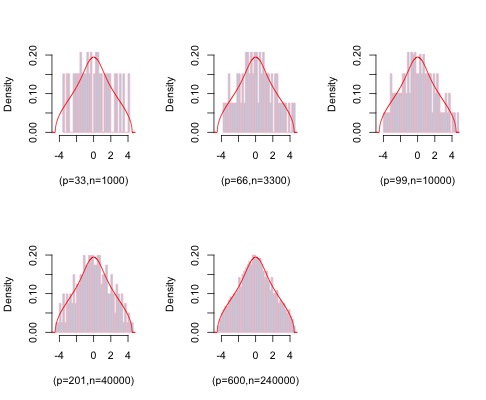
and solve the equations bยฏ0=0.5โ€‹ฮฒ1+0.5โ€‹ฮฒ2\bar{b}^{0}=0.5\beta_{1}+0.5\beta_{2} and bยฏ20=0.5โ€‹ฮฒ12+0.5โ€‹ฮฒ22\bar{b}_{2}^{0}=0.5\beta_{1}^{2}+0.5\beta_{2}^{2} to obtain ฮฒ1\beta_{1} and ฮฒ2\beta_{2}. In Section 5 we conduct a simulation study which shows that the the histogram of the LSD of Cnโ€‹0C_{n0} is very close to the theoretical density function 2.5 of the LSD FA0,B0โ€‹(x)F^{A_{0},B_{0}}(x) under H0H_{0}. In addition, the distribution of LnL_{n} under H0H_{0} and H1H_{1} are well-separated as p,nโ†’โˆžp,n\to\infty and p/nโ†’0p/n\to 0. We do not present simulation results involving the statistic VnV_{n} due to space constraints, even though the qualitative behavior is similar.

Even though the proposed procedure does not test the separability of the covariance matrix of the data, we comment on the possibility of extending this test procedure to deal with some special cases of the latter scenario. The implementation of these is beyond the scope of this paper. The corresponding null hypothesis for the test of separability would be: H0:ฮฃn=ApโŠ—BnH_{0}:\Sigma_{n}=A_{p}\otimes B_{n} where ApA_{p} and BnB_{n} are unknown positive semi-definite matrices satisfying that the ESD FApF^{A_{p}} converges to a distribution non-degenerate at zero, and nโˆ’1โ€‹trโ€‹(Bn)โ†’1n^{-1}\mbox{tr}(B_{n})\to 1 and nโˆ’1โ€‹trโ€‹(Bn2)โ†’bยฏ2n^{-1}\mbox{tr}(B_{n}^{2})\to\bar{b}_{2} for some bยฏ2โ‰ฅ1\bar{b}_{2}\geq 1. The requirement nโˆ’1โ€‹trโ€‹(Bn)โ†’1n^{-1}\mbox{tr}(B_{n})\to 1 is to ensure identifiability. In this case, under certain special structural assumptions on ApA_{p}, it may still be possible to obtain fairly accurate estimates of ApA_{p} and bยฏ2\bar{b}_{2}, which can then be used in the expression for LnL_{n} or VnV_{n} in place of A0A_{0} and bยฏ20\bar{b}_{2}^{0} to construct a test for separability. One typical assumption in spatio-temporal statistics is that the process is stationary either in space or time. In the current setting, if we assume that the process is row-stationary, then the eigenvectors of ApA_{p} can be well-approximated in a discrete Fourier basis. If in addition, the corresponding spectrum of ApA_{p} is piecewise constant, then we can estimate the spectrum of ApA_{p} from the data as follows. First we can perform an orthogonal or unitary transformation of the data in the (approximate) eigen-basis of ApA_{p}. Then, we can apply a clustering procedure, and estimate the distinct eigenvalues as the means of the individual clusters, and assign the eigenvectors to these clusters according to the cluster membership of the coordinates of the rotated data matrix. Another way to broaden the class of models under the null hypothesis is to remove the specification of bยฏ2\bar{b}_{2}. If either the eigenvalues of ApA_{p} are known or they can be estimated accurately from the data, subject to some knowledge about the fourth moment of the entries of the data matrix, bยฏ2\bar{b}_{2} can be estimated by making use of the expression for ๐”ผโ€‹(trโ€‹(Sn2))\mathbb{E}(\mbox{tr}(S_{n}^{2})) in terms of the first two spectral moments of ApA_{p} and BnB_{n}.

If ApA_{p} is unknown but has a relatively small number of distinct eigenvalues, those eigenvalues can be estimated as mean or median of the clusters of eigenvalues of SnS_{n}, without requiring any knowledge of the eigenvectors of ApA_{p}, by making use of Theorem 2.8.

2.4 Computation of the density function of the LSD

If FAF^{A} is a finite mixture of point masses, then the density function of the LSD FF in Theorem 2.1 can be computed numerically by making use of Proposition 2.6 and Lemma 2.7. This computation is used to simulate the distribution of the test statistic LnL_{n} in Section 5. According to 2.6, the main ingredient of the computation of ff, the p.d.f. of FF, is the determination of the function ฮฒโก(x):=limzโˆˆโ„‚+โ†’xฮฒโก(z)\beta(x):=\lim_{z\in\mathbb{C}^{+}\to x}\beta(z) which solves the equation (2.3). When FAF^{A} is a finite mixture of point masses, the latter reduces to a polynomial in ฮฒโก(x)\beta(x). In order to determine fโก(x)f(x), we need to isolate the roots that satisfy the constraints โ„‘โกฮฒโก(x)โ‰ฅ0\Im\beta(x)\geq 0, xโ€‹โ„œโกฮฒโ€‹(x)<0x\Re\beta(x)<0 and ฯ‰โก(x)โ‰ค1\omega(x)\leq 1, where ฯ‰โก(x)\omega(x) is given by (2.4), as stated in Proposition 2.6. Indeed, the support of ฮฒโก(x)\beta(x) can be determined by the condition ฯ‰โก(x)=1\omega(x)=1, as stated in Lemma 2.7. In practice, we numerically solve for the appropriate root of ฮฒโก(x)\beta(x) for a grid of points xx by searching through all possible solutions of the polynomial satisfied by ฮฒโก(x)\beta(x) and checking the conditions, as well as making use of the continuity of ฮฒโก(x)\beta(x) on each side of the origin. Then we can derive the density function fโก(x)f(x) by utilizing (2.5).

3 Proof of Theorem 2.1

Our approach for proving Theorem 2.1 is to first restrict to Gaussian observations and utilize the rank-one perturbation method used in Bai and Yin [3] and Pan and Gao [20]. However, the decompositions under the separable case require a slightly different treatment from the aforementioned references. The extension of the result to non-Gausssian settings is handled in Section 3.5 through through a use of the Lindeberg principle (see Chatterjee [6]). Another potential route to prove this result is through the generalized Steinโ€™s equations used in Pastur and Shcherbina [19] and Bao [5].

3.1 Truncation of the ESD of ApA_{p}

We begin with a truncation of the spectrum of ApA_{p}. Let b0b_{0} be a positive number such that โ€–Bnโ€–โ‰คb0\|B_{n}\|\leq b_{0}. Define bยฏn=trโ€‹(Bn)/n\bar{b}_{n}=\mbox{tr}(B_{n})/n and suppose that bยฏnโ†’bยฏ\bar{b}_{n}\to\bar{b} as nโ†’โˆžn\to\infty. Let a0>0a_{0}>0 be such that a0a_{0} is a continuity point of FAF^{A}, the LSD of ApA_{p}. Let

ฮ›a0=diag(ฮป1I{ฮป1โ‰คa0},ฮป2I{ฮป2โ‰คa0},โ‹ฏ,ฮปpI{ฮปpโ‰คa0}).\Lambda_{a_{0}}=\mbox{diag}\left(\lambda_{1}I_{\{\lambda_{1}\leq a_{0}\}},\lambda_{2}I_{\{\lambda_{2}\leq a_{0}\}},\cdots,\lambda_{p}I_{\{\lambda_{p}\leq a_{0}\}}\right).

Since Ap=Uโˆ—โ€‹ฮ›โ€‹UA_{p}=U^{*}\Lambda U with ฮ›=diagโ€‹(ฮป1,ฮป2,โ‹ฏ,ฮปp)\Lambda=\mbox{diag}(\lambda_{1},\lambda_{2},\cdots,\lambda_{p}), then defining A~a0:=Uโˆ—โ€‹ฮ›a0โ€‹U\widetilde{A}_{a_{0}}:=U^{*}\Lambda_{a_{0}}U, A~a01/2:=Uโˆ—โ€‹ฮ›a01/2โ€‹U\widetilde{A}_{a_{0}}^{1/2}:=U^{*}\Lambda_{a_{0}}^{1/2}U, and C~nโ€‹0:=n/pโ€‹(nโˆ’1โ€‹Ap1/2โ€‹Xnโ€‹Bnโ€‹Xnโˆ—โ€‹Ap1/2โˆ’nโˆ’1โ€‹trโ€‹(Bn)โ€‹A~a0)\widetilde{C}_{n0}:=\sqrt{n/p}\left(n^{-1}A_{p}^{1/2}X_{n}B_{n}X_{n}^{*}A_{p}^{1/2}-n^{-1}\mbox{tr}(B_{n})\widetilde{A}_{a_{0}}\right), we have

supx|FCnโ€‹(x)โˆ’FC~nโ€‹0โ€‹(x)|\displaystyle\sup_{x}\left|F^{C_{n}}(x)-F^{\widetilde{C}_{n0}}(x)\right|
โ‰คbยฏnpRank(Apโˆ’A~a0)=bยฏnpโˆ‘i=1pI{ฮปi>a0}โ†’bยฏ(1โˆ’FA(a0)).\displaystyle\leq\frac{\bar{b}_{n}}{p}\mbox{Rank}\left(A_{p}-\widetilde{A}_{a_{0}}\right)=\frac{\bar{b}_{n}}{p}\sum_{i=1}^{p}I_{\{\lambda_{i}>a_{0}\}}\rightarrow\bar{b}\left(1-F^{A}(a_{0})\right).

Further, defining C^nโ€‹0:=npโ€‹(1nโ€‹A~a01/2โ€‹Xnโ€‹Bnโ€‹Xnโˆ—โ€‹A~a01/2โˆ’trโ€‹(Bn)nโ€‹A~a0)\widehat{C}_{n0}:=\sqrt{\frac{n}{p}}\left(\frac{1}{n}\widetilde{A}_{a_{0}}^{1/2}X_{n}B_{n}X_{n}^{*}\widetilde{A}_{a_{0}}^{1/2}-\frac{\mbox{tr}(B_{n})}{n}\widetilde{A}_{a_{0}}\right), we have

supx|FC~nโ€‹0โ€‹(x)โˆ’FC^nโ€‹0โ€‹(x)|\displaystyle\sup_{x}\left|F^{\widetilde{C}_{n0}}(x)-F^{\widehat{C}_{n0}}(x)\right|
โ‰ค2pRank(Ap1/2โˆ’A~a01/2)=2pโˆ‘i=1pI{ฮปi>a0}โ†’2(1โˆ’FA(a0)).\displaystyle\leq\frac{2}{p}\mbox{Rank}(A_{p}^{1/2}-\widetilde{A}_{a_{0}}^{1/2})=\frac{2}{p}\sum_{i=1}^{p}I_{\{\lambda_{i}>a_{0}\}}\to 2(1-F^{A}(a_{0})).

By choosing a0a_{0} to be large enough, 1โˆ’FAโ€‹(a0)1-F^{A}(a_{0}) can be made arbitrarily small. Thus, combining the above two inequalities, we can show that, for any given ฯต>0\epsilon>0, there exists a large enough a0a_{0} such that

limsupnโ†’โˆžsupx|FCnโ€‹(x)โˆ’FC^nโ€‹0โ€‹(x)|โ‰คฯตa.s.\lim\sup_{n\to\infty}\sup_{x}\left|F^{C_{n}}(x)-F^{\widehat{C}_{n0}}(x)\right|\leq\epsilon\qquad\mbox{a.s.}

Also, in Section 3.4, we show that the solution of (2.1) is unique and has a continuous dependence on FAF^{A}. Thus, since FA~a0F^{\widetilde{A}_{a_{0}}} converges to FAF^{A} in distribution as a0โ†’โˆža_{0}\to\infty, in order to prove Theorem 2.1, it is enough to show that FC^nโ€‹0F^{\widehat{C}_{n0}} converges almost surely to FF, and FF has the Stieltjes transform sโก(z)s(z) determined by (2.1) with FA=FA~a0F^{A}=F^{\widetilde{A}_{a_{0}}}, for any fixed positive a0a_{0} so that FA~a0F^{\widetilde{A}_{a_{0}}} is not degenerate at zero. For notational convenience, henceforth, we still use ApA_{p} and CnC_{n} instead of A~a0\widetilde{A}_{a_{0}} and C^nโ€‹0\widehat{C}_{n0}, respectively, and simply assume that of โˆฅApโˆฅโ‰คa0\parallel A_{p}\parallel\leq a_{0} for an arbitrary positive constant a0a_{0}.

3.2 Expected Stieltjes transforms

In this subsection, we derive asymptotic expansion for ๐”ผโ€‹(snโ€‹(z))\mathbb{E}(s_{n}(z)) when XnX_{n} is assumed to have i.i.d. standard normal entries. Let Ap=Uโˆ—โ€‹ฮ›โ€‹UA_{p}=U^{*}\Lambda U with ฮ›=diagโ€‹(ฮป1,ฮป2,โ‹ฏ,ฮปp)\Lambda=\mbox{diag}(\lambda_{1},\lambda_{2},\cdots,\lambda_{p}) denoting the spectral decomposition of ApA_{p}. Then we have

Cn\displaystyle C_{n} =\displaystyle= npโ€‹(1nโ€‹Uโˆ—โ€‹ฮ›1/2โ€‹Uโ€‹Xnโ€‹Bnโ€‹Xnโˆ—โ€‹Uโˆ—โ€‹ฮ›1/2โ€‹Uโˆ’1nโ€‹trโ€‹(Bn)โ€‹Uโˆ—โ€‹ฮ›โ€‹U)\displaystyle\sqrt{\frac{n}{p}}\left(\frac{1}{n}U^{*}\Lambda^{1/2}UX_{n}B_{n}X_{n}^{*}U^{*}\Lambda^{1/2}U-\frac{1}{n}\mbox{tr}(B_{n})U^{*}\Lambda U\right)
=\displaystyle= npโ€‹Uโˆ—โ€‹(1nโ€‹ฮ›1/2โ€‹Uโ€‹Xnโ€‹Bnโ€‹Xnโˆ—โ€‹Uโˆ—โ€‹ฮ›1/2โˆ’1nโ€‹trโ€‹(Bn)โ€‹ฮ›)โ€‹U\displaystyle\sqrt{\frac{n}{p}}U^{*}\left(\frac{1}{n}\Lambda^{1/2}UX_{n}B_{n}X_{n}^{*}U^{*}\Lambda^{1/2}-\frac{1}{n}\mbox{tr}(B_{n})\Lambda\right)U
=\displaystyle= npโ€‹Uโˆ—โ€‹(1nโ€‹ฮ›1/2โ€‹X~nโ€‹Bnโ€‹X~nโˆ—โ€‹ฮ›1/2โˆ’1nโ€‹trโ€‹(Bn)โ€‹ฮ›)โ€‹U\displaystyle\sqrt{\frac{n}{p}}U^{*}\left(\frac{1}{n}\Lambda^{1/2}\widetilde{X}_{n}B_{n}\widetilde{X}_{n}^{*}\Lambda^{1/2}-\frac{1}{n}\mbox{tr}(B_{n})\Lambda\right)U
=\displaystyle= npโ€‹Uโˆ—โ€‹(Vโ€‹Vโˆ—โˆ’bยฏnโ€‹ฮ›)โ€‹U\displaystyle\sqrt{\frac{n}{p}}U^{*}(VV^{*}-\bar{b}_{n}\Lambda)U

where X~n=Uโ€‹Xn\widetilde{X}_{n}=UX_{n} and V=nโˆ’1/2ฮ›1/2X~nBn1/2V=n^{-1/2}\Lambda^{1/2}\widetilde{X}_{n}B_{n}^{1/2}. Let vk=nโˆ’1/2ฮปkBn1/2x~kv_{k}=n^{-1/2}\sqrt{\lambda_{k}}B_{n}^{1/2}\widetilde{x}_{k} denote the kk-th column of Vโˆ—V^{*}, where x~k\widetilde{x}_{k} is the kk-th column of X~nโˆ—.\widetilde{X}_{n}^{*}. Note that X~n\widetilde{X}_{n} has i.i.d Gaussian entries with mean zero and variance one. Moreover, denote by X~(k)\widetilde{X}_{(k)} the matrix obtained from X~n\widetilde{X}_{n} with the kk-th row replaced by zero. Then

V(k)=(v1โˆ—,โ‹ฏ,vkโˆ’1โˆ—,0,vk+1โˆ—,โ‹ฏ,vpโˆ—)โˆ—.V_{(k)}=(v_{1}^{*},\cdots,v_{k-1}^{*},0,v_{k+1}^{*},\cdots,v_{p}^{*})^{*}.

We introduce the following quantities:

ฯ‰k\displaystyle\omega_{k} =\displaystyle= npโ€‹V(k)โ€‹vk\displaystyle\sqrt{\frac{n}{p}}V_{(k)}v_{k}
ฯ„kโ€‹k\displaystyle\tau_{kk} =\displaystyle= npโ€‹(vkโˆ—โ€‹vkโˆ’bยฏnโ€‹ฮปk),\displaystyle\sqrt{\frac{n}{p}}(v_{k}^{*}v_{k}-\bar{b}_{n}\lambda_{k}),
Yโก(z)\displaystyle Y(z) =\displaystyle= npโ€‹(Vโ€‹Vโˆ—โˆ’bยฏnโ€‹ฮ›)โˆ’zโ€‹I,\displaystyle\sqrt{\frac{n}{p}}\left(VV^{*}-\bar{b}_{n}\Lambda\right)-zI,
Ykโ€‹(z)\displaystyle Y_{k}(z) =\displaystyle= npโ€‹(V(k)โ€‹Vโˆ—โˆ’bยฏnโ€‹ฮ›(k))โˆ’zโ€‹I,\displaystyle\sqrt{\frac{n}{p}}\left(V_{(k)}V^{*}-\bar{b}_{n}\Lambda_{(k)}\right)-zI,
Y(k)โ€‹(z)\displaystyle Y_{(k)}(z) =\displaystyle= npโ€‹(V(k)โ€‹V(k)โˆ—โˆ’bยฏnโ€‹ฮ›(k))โˆ’zโ€‹I,\displaystyle\sqrt{\frac{n}{p}}\left(V_{(k)}V_{(k)}^{*}-\bar{b}_{n}\Lambda_{(k)}\right)-zI,
hk\displaystyle h_{k} =\displaystyle= ฯ‰k+ฯ„kโ€‹kโ€‹ek.\displaystyle\omega_{k}+\tau_{kk}e_{k}.

Where eke_{k} is supposed to be a canonical unit pร—1p\times 1 vector with the kk-th element being 11 and all others 00. Then, notice that Yโก(z)=โˆ‘k=1pekโ€‹hkโˆ—=Ykโ€‹(z)+ekโ€‹hkโˆ—Y(z)=\sum_{k=1}^{p}e_{k}h_{k}^{*}=Y_{k}(z)+e_{k}h_{k}^{*}, for all kk. Thus, Cn=Uโˆ—โ€‹Yโ€‹(z)โ€‹U=Uโˆ—โ€‹(โˆ‘k=1pekโ€‹hkโˆ—)โ€‹UC_{n}=U^{*}Y(z)U=U^{*}\left(\sum_{k=1}^{p}e_{k}h_{k}^{*}\right)U. Since, (Cnโˆ’zโ€‹I)โˆ’1=โˆ’zโˆ’1โ€‹I+zโˆ’1โ€‹Cnโ€‹(Cnโˆ’zโ€‹I)โˆ’1(C_{n}-zI)^{-1}=-z^{-1}I+z^{-1}C_{n}(C_{n}-zI)^{-1}, we have

snโ€‹(z)\displaystyle s_{n}(z) =\displaystyle= 1pโ€‹trโ€‹(Cnโˆ’zโ€‹I)โˆ’1\displaystyle\frac{1}{p}\mbox{tr}(C_{n}-zI)^{-1} (3.1)
=\displaystyle= zโˆ’1pโ€‹trโ€‹(Cnโ€‹(Cnโˆ’zโ€‹I)โˆ’1)โˆ’zโˆ’1\displaystyle\frac{z^{-1}}{p}\mbox{tr}\left(C_{n}(C_{n}-zI)^{-1}\right)-z^{-1}
=\displaystyle= zโˆ’1pโ€‹trโ€‹(โˆ‘k=1pekโ€‹hkโˆ—โ€‹(npโ€‹(Vโ€‹Vโˆ—โˆ’bยฏnโ€‹ฮ›)โˆ’zโ€‹I)โˆ’1)โˆ’zโˆ’1\displaystyle\frac{z^{-1}}{p}\mbox{tr}\left(\sum_{k=1}^{p}e_{k}h_{k}^{*}\left(\sqrt{\frac{n}{p}}(VV^{*}-\bar{b}_{n}\Lambda)-zI\right)^{-1}\right)-z^{-1}
=\displaystyle= zโˆ’1pโ€‹trโ€‹(โˆ‘k=1pekโ€‹hkโˆ—โ€‹(Ykโ€‹(z)+ekโ€‹hkโˆ—)โˆ’1)โˆ’zโˆ’1\displaystyle\frac{z^{-1}}{p}\mbox{tr}\left(\sum_{k=1}^{p}e_{k}h_{k}^{*}\left(Y_{k}(z)+e_{k}h_{k}^{*}\right)^{-1}\right)-z^{-1}
=\displaystyle= zโˆ’1pโ€‹trโ€‹(โˆ‘k=1pekโ€‹hkโˆ—โ€‹(Ykโˆ’1โ€‹(z)โˆ’Ykโˆ’1โ€‹(z)โ€‹ekโ€‹hkโˆ—โ€‹Ykโˆ’1โ€‹(z)1+hkโˆ—โ€‹Ykโˆ’1โ€‹(z)โ€‹ek))โˆ’zโˆ’1\displaystyle\frac{z^{-1}}{p}\mbox{tr}\left(\sum_{k=1}^{p}e_{k}h_{k}^{*}\left(Y_{k}^{-1}(z)-\frac{Y_{k}^{-1}(z)e_{k}h_{k}^{*}Y_{k}^{-1}(z)}{1+h_{k}^{*}Y_{k}^{-1}(z)e_{k}}\right)\right)-z^{-1}
=\displaystyle= zโˆ’1pโ€‹โˆ‘k=1phkโˆ—โ€‹Ykโˆ’1โ€‹(z)โ€‹ek1+hkโˆ—โ€‹Ykโˆ’1โ€‹(z)โ€‹ekโˆ’zโˆ’1\displaystyle\frac{z^{-1}}{p}\sum_{k=1}^{p}\frac{h_{k}^{*}Y_{k}^{-1}(z)e_{k}}{1+h_{k}^{*}Y_{k}^{-1}(z)e_{k}}-z^{-1}
=\displaystyle= โˆ’zโˆ’1pโˆ‘k=1p11+hkโˆ—โ€‹Ykโˆ’1โ€‹(z)โ€‹ek\displaystyle-\frac{z^{-1}}{p}\sum_{k=1}^{p}\frac{1}{1+h_{k}^{*}Y_{k}^{-1}(z)e_{k}}

From the structure of Ykโ€‹(z),Y(k)โ€‹(z)Y_{k}(z),Y_{{(k)}}(z) and ฯ‰k\omega_{k}, we observe that

Ykโˆ’1โ€‹(z)=(Y(k)โ€‹(z)+ฯ‰kโ€‹ekT)โˆ’1,Y(k)โˆ’1โ€‹(z)โ€‹ek=โˆ’zโˆ’1โ€‹ek,ฯ‰kโˆ—โ€‹ek=ekTโ€‹ฯ‰k=npโ€‹ekTโ€‹V(k)โ€‹vk=0.Y_{k}^{-1}(z)=\left(Y_{(k)}(z)+\omega_{k}e_{k}^{T}\right)^{-1},~~~Y_{(k)}^{-1}(z)e_{k}=-z^{-1}e_{k},~~~~\omega_{k}^{*}e_{k}=e_{k}^{T}\omega_{k}=\sqrt{\frac{n}{p}}e_{k}^{T}V_{(k)}v_{k}=0. (3.2)

For any non-negative definite pร—pp\times p Hermitian matrix DD, define Dยฏ=Uโ€‹Dโ€‹Uโˆ—={dยฏiโ€‹j}\underline{D}=UDU^{*}=\{\underline{d}_{ij}\}. Then it follows that

hkโˆ—โ€‹Ykโˆ’1โ€‹(z)โ€‹Dยฏโ€‹ek\displaystyle h_{k}^{*}Y_{k}^{-1}(z)\underline{D}e_{k} =\displaystyle= hkโˆ—โ€‹(Y(k)โˆ’1โ€‹(z)โˆ’Y(k)โˆ’1โ€‹(z)โ€‹ฯ‰kโ€‹ekTโ€‹Y(k)โˆ’1โ€‹(z)1+ekTโ€‹Y(k)โˆ’1โ€‹(z)โ€‹ฯ‰k)โ€‹Dยฏโ€‹ek\displaystyle h_{k}^{*}\left(Y_{(k)}^{-1}(z)-\frac{Y_{(k)}^{-1}(z)\omega_{k}e_{k}^{T}Y_{(k)}^{-1}(z)}{1+e_{k}^{T}Y_{(k)}^{-1}(z)\omega_{k}}\right)\underline{D}e_{k} (3.3)
=\displaystyle= hkโˆ—โ€‹(Y(k)โˆ’1โ€‹(z)+1zโ€‹Y(k)โˆ’1โ€‹(z)โ€‹ฯ‰kโ€‹ekT)โ€‹Dยฏโ€‹ek\displaystyle h_{k}^{*}\left(Y_{(k)}^{-1}(z)+\frac{1}{z}Y_{(k)}^{-1}(z)\omega_{k}e_{k}^{T}\right)\underline{D}e_{k}
=\displaystyle= hkโˆ—โ€‹Y(k)โˆ’1โ€‹(z)โ€‹Dยฏโ€‹ek+1zโ€‹hkโˆ—โ€‹Y(k)โˆ’1โ€‹(z)โ€‹ฯ‰kโ€‹ekTโ€‹Dยฏโ€‹ek\displaystyle h_{k}^{*}Y_{(k)}^{-1}(z)\underline{D}e_{k}+\frac{1}{z}h_{k}^{*}Y_{(k)}^{-1}(z)\omega_{k}e_{k}^{T}\underline{D}e_{k}
=\displaystyle= 1zโ€‹[dยฏkโ€‹kโ€‹ฯ‰kโˆ—โ€‹Y(k)โˆ’1โ€‹(z)โ€‹ฯ‰kโˆ’ฯ„kโ€‹kโ€‹dยฏkโ€‹k]+ฯ‰kโˆ—โ€‹Y(k)โˆ’1โ€‹(z)โ€‹Dยฏโ€‹ek\displaystyle\frac{1}{z}\left[\underline{d}_{kk}\omega_{k}^{*}Y_{(k)}^{-1}(z)\omega_{k}-\tau_{kk}\underline{d}_{kk}\right]+\omega_{k}^{*}Y_{(k)}^{-1}(z)\underline{D}e_{k}
:โฃ=\displaystyle:= I+Iโ€‹I.\displaystyle I+II.

When D=ID=I, the term Iโ€‹III in (3.3) equals zero since by (3.2), ฯ‰kโˆ—โ€‹Y(k)โˆ’1โ€‹(z)โ€‹ek=โˆ’zโˆ’1โ€‹ฯ‰kโˆ—โ€‹ek=0\omega_{k}^{*}Y_{(k)}^{-1}(z)e_{k}=-z^{-1}\omega_{k}^{*}e_{k}=0. Plugging this into (3.1), and using dยฏkโ€‹k=1\underline{d}_{kk}=1, we get

sn(z)=โˆ’1pโˆ‘k=1p1zโˆ’ฯ„kโ€‹k+ฯ‰kโˆ—โ€‹Y(k)โˆ’1โ€‹(z)โ€‹ฯ‰k.s_{n}(z)=-\frac{1}{p}\sum_{k=1}^{p}\frac{1}{z-\tau_{kk}+\omega_{k}^{*}Y_{(k)}^{-1}(z)\omega_{k}}. (3.4)

Moreover, with the expression given by (3.1) and (3.3), we similarly have

1pโ€‹trโ€‹((Cnโˆ’zโ€‹I)โˆ’1โ€‹D)\displaystyle\frac{1}{p}\mbox{tr}\left((C_{n}-zI)^{-1}D\right) =\displaystyle= zโˆ’1pโ€‹trโ€‹(Cnโ€‹(Cnโˆ’zโ€‹I)โˆ’1โ€‹D)โˆ’zโˆ’1pโ€‹trโ€‹(D)\displaystyle\frac{z^{-1}}{p}\mbox{tr}\left(C_{n}(C_{n}-zI)^{-1}D\right)-\frac{z^{-1}}{p}\mbox{tr}(D) (3.5)
=\displaystyle= zโˆ’1pโ€‹โˆ‘k=1phkโˆ—โ€‹Ykโˆ’1โ€‹(z)โ€‹Dยฏโ€‹ek1+hkโˆ—โ€‹Ykโˆ’1โ€‹(z)โ€‹ekโˆ’zโˆ’1pโ€‹trโ€‹(Dยฏ)\displaystyle\frac{z^{-1}}{p}\sum_{k=1}^{p}\frac{h_{k}^{*}Y_{k}^{-1}(z)\underline{D}e_{k}}{1+h_{k}^{*}Y_{k}^{-1}(z)e_{k}}-\frac{z^{-1}}{p}\mbox{tr}(\underline{D})
=\displaystyle= zโˆ’1pโ€‹โˆ‘k=1pdยฏkโ€‹kโ€‹ฯ‰kโˆ—โ€‹Y(k)โˆ’1โ€‹(z)โ€‹ฯ‰kโˆ’ฯ„kโ€‹kโ€‹dยฏkโ€‹kzโˆ’ฯ„kโ€‹k+ฯ‰kโˆ—โ€‹Y(k)โˆ’1โ€‹(z)โ€‹ฯ‰kโˆ’zโˆ’1pโ€‹trโ€‹(Dยฏ).\displaystyle\frac{z^{-1}}{p}\sum_{k=1}^{p}\frac{\underline{d}_{kk}\omega_{k}^{*}Y_{(k)}^{-1}(z)\omega_{k}-\tau_{kk}\underline{d}_{kk}}{z-\tau_{kk}+\omega_{k}^{*}Y_{(k)}^{-1}(z)\omega_{k}}-\frac{z^{-1}}{p}\mbox{tr}(\underline{D}).

Define

ฮฒnโ€‹(z)=1pโ€‹trโ€‹((Cnโˆ’zโ€‹I)โˆ’1โ€‹Ap),zโˆˆโ„‚+.\beta_{n}(z)=\frac{1}{p}\mbox{tr}\left((C_{n}-zI)^{-1}A_{p}\right),~~~z\in\mathbb{C}^{+}. (3.6)

When D=ApD=A_{p}, so that Dยฏ=ฮ›=dโ€‹iโ€‹aโ€‹gโ€‹(ฮป1,ฮป2,โ‹ฏ,ฮปp)\underline{D}=\Lambda=diag(\lambda_{1},\lambda_{2},\cdots,\lambda_{p}), from (3.5), we get

ฮฒnโ€‹(z)\displaystyle\beta_{n}(z) =\displaystyle= zโˆ’1pโ€‹trโ€‹(โˆ‘k=1phkโˆ—โ€‹Ykโˆ’1โ€‹(z)โ€‹ฮ›โ€‹ek1+hkโˆ—โ€‹Ykโˆ’1โ€‹(z)โ€‹ek)โˆ’zโˆ’1pโ€‹trโ€‹(ฮ›)\displaystyle\frac{z^{-1}}{p}\mbox{tr}\left(\sum_{k=1}^{p}\frac{h_{k}^{*}Y_{k}^{-1}(z)\Lambda e_{k}}{1+h_{k}^{*}Y_{k}^{-1}(z)e_{k}}\right)-\frac{z^{-1}}{p}\mbox{tr}(\Lambda) (3.7)
=\displaystyle= zโˆ’1pโ€‹โˆ‘k=1pฮปkโ€‹ฯ‰kโˆ—โ€‹Y(k)โˆ’1โ€‹(z)โ€‹ฯ‰kโˆ’ฯ„kโ€‹kโ€‹ฮปkzโˆ’ฯ„kโ€‹k+ฯ‰kโˆ—โ€‹Y(k)โˆ’1โ€‹(z)โ€‹ฯ‰kโˆ’zโˆ’1pโ€‹โˆ‘k=1pฮปk\displaystyle\frac{z^{-1}}{p}\sum_{k=1}^{p}\frac{\lambda_{k}\omega_{k}^{*}Y_{(k)}^{-1}(z)\omega_{k}-\tau_{kk}\lambda_{k}}{z-\tau_{kk}+\omega_{k}^{*}Y_{(k)}^{-1}(z)\omega_{k}}-\frac{z^{-1}}{p}\sum_{k=1}^{p}\lambda_{k}
=\displaystyle= โˆ’1pโˆ‘k=1pฮปkzโˆ’ฯ„kโ€‹k+ฯ‰kโˆ—โ€‹Y(k)โˆ’1โ€‹(z)โ€‹ฯ‰k.\displaystyle-\frac{1}{p}\sum_{k=1}^{p}\frac{\lambda_{k}}{z-\tau_{kk}+\omega_{k}^{*}Y_{(k)}^{-1}(z)\omega_{k}}~.

In order to derive explicit expressions for snโ€‹(z)s_{n}(z) and ฮฒnโ€‹(z)\beta_{n}(z), we still need a further approximation of ฯ‰kโˆ—โ€‹Y(k)โˆ’1โ€‹(z)โ€‹ฯ‰k\omega_{k}^{*}Y_{(k)}^{-1}(z)\omega_{k}. Indeed,

ฯ‰kโˆ—โ€‹Y(k)โˆ’1โ€‹(z)โ€‹ฯ‰k\displaystyle\omega_{k}^{*}Y_{(k)}^{-1}(z)\omega_{k} =\displaystyle= npโ€‹vkโˆ—โ€‹V(k)โˆ—โ€‹Y(k)โˆ’1โ€‹(z)โ€‹V(k)โ€‹vk\displaystyle\frac{n}{p}v_{k}^{*}V_{(k)}^{*}Y_{(k)}^{-1}(z)V_{(k)}v_{k} (3.8)
=\displaystyle= ฮปkpโ€‹trโ€‹(V(k)โ€‹Bn1/2โ€‹x~kโ€‹x~kโˆ—โ€‹Bn1/2โ€‹V(k)โˆ—โ€‹Y(k)โˆ’1โ€‹(z))\displaystyle\frac{\lambda_{k}}{p}\mbox{tr}\left(V_{(k)}B_{n}^{1/2}\widetilde{x}_{k}\widetilde{x}_{k}^{*}B_{n}^{1/2}V_{(k)}^{*}Y_{(k)}^{-1}(z)\right)
=\displaystyle= ฮปkpโ€‹trโ€‹(V(k)โ€‹Bnโ€‹V(k)โˆ—โ€‹Y(k)โˆ’1โ€‹(z))+dk(1)\displaystyle\frac{\lambda_{k}}{p}\mbox{tr}\left(V_{(k)}B_{n}V_{(k)}^{*}Y_{(k)}^{-1}(z)\right)+d_{k}^{(1)}
=\displaystyle= ฮปkpโ€‹nโ€‹trโ€‹(ฮ›1/2โ€‹X~(k)โ€‹Bn2โ€‹X~(k)โˆ—โ€‹ฮ›1/2โ€‹Y(k)โˆ’1โ€‹(z))+dk(1)\displaystyle\frac{\lambda_{k}}{pn}\mbox{tr}\left(\Lambda^{1/2}\widetilde{X}_{(k)}B_{n}^{2}\widetilde{X}_{(k)}^{*}\Lambda^{1/2}Y_{(k)}^{-1}(z)\right)+d_{k}^{(1)}
=\displaystyle= ฮปkpโ€‹nโ€‹โˆ‘i,jโ‰ k(ฮปiโ€‹ฮปjโ€‹x~iโˆ—โ€‹Bn2โ€‹x~j)โ€‹(Y(k)โˆ’1โ€‹(z))jโ€‹i+dk(1)\displaystyle\frac{\lambda_{k}}{pn}\sum_{i,j\neq k}\left(\sqrt{\lambda_{i}\lambda_{j}}\widetilde{x}_{i}^{*}B_{n}^{2}\widetilde{x}_{j}\right)\left(Y_{(k)}^{-1}(z)\right)_{ji}+d_{k}^{(1)}
=\displaystyle= ฮปkโ€‹trโ€‹(Bn2)pโ€‹nโ€‹โˆ‘iโ‰ k(ฮปiโ€‹(Y(k)โˆ’1โ€‹(z))iโ€‹i)+dk(2)\displaystyle\frac{\lambda_{k}\mbox{tr}(B_{n}^{2})}{pn}\sum_{i\neq k}\left(\lambda_{i}(Y_{(k)}^{-1}(z))_{ii}\right)+d_{k}^{(2)}
=\displaystyle= bยฏ2โ€‹(n)โ€‹ฮปkpโ€‹trโ€‹(Y(k)โˆ’1โ€‹(z)โ€‹ฮ›(k))+dk(2)\displaystyle\bar{b}_{2}(n)\frac{\lambda_{k}}{p}\mbox{tr}\left(Y_{(k)}^{-1}(z)\Lambda_{(k)}\right)+d_{k}^{(2)}

where ๐”ผโก(dk(1))=0\mathbb{E}(d_{k}^{(1)})=0 and ๐”ผโก(dk(2))=0\mathbb{E}(d_{k}^{(2)})=0. Note that

1pโ€‹trโ€‹(Y(k)โˆ’1โ€‹(z)โ€‹ฮ›(k))โ‰ˆ1pโ€‹trโ€‹(Yโˆ’1โ€‹(z)โ€‹ฮ›)=1pโ€‹trโ€‹((Cnโˆ’zโ€‹I)โˆ’1โ€‹Ap)=ฮฒnโ€‹(z),\frac{1}{p}\mbox{tr}\left(Y_{(k)}^{-1}(z)\Lambda_{(k)}\right)\approx\frac{1}{p}\mbox{tr}\left(Y^{-1}(z)\Lambda\right)=\frac{1}{p}\mbox{tr}\left((C_{n}-zI)^{-1}A_{p}\right)=\beta_{n}(z),

which shows that the term ฯ‰kโˆ—โ€‹Y(k)โˆ’1โ€‹(z)โ€‹ฯ‰k\omega_{k}^{*}Y_{(k)}^{-1}(z)\omega_{k} in (3.7) can be approximated by bยฏ2โ€‹(n)โ€‹ฮปkโ€‹๐”ผโ€‹(ฮฒnโ€‹(z))\bar{b}_{2}(n)\lambda_{k}\mathbb{E}(\beta_{n}(z)). Hence we can derive convenient representations for ๐”ผโ€‹(snโ€‹(z))\mathbb{E}(s_{n}(z)) and ๐”ผโ€‹(ฮฒnโ€‹(z))\mathbb{E}(\beta_{n}(z)) though this approximation and show that the remainder terms are negligible.

Let

ฯตk:=bยฏ2โ€‹(n)โ€‹ฮปkโ€‹๐”ผโ€‹(ฮฒnโ€‹(z))โˆ’ฯ‰kโˆ—โ€‹Y(k)โˆ’1โ€‹(z)โ€‹ฯ‰k+ฯ„kโ€‹k.\epsilon_{k}:=\bar{b}_{2}(n)\lambda_{k}\mathbb{E}(\beta_{n}(z))-\omega_{k}^{*}Y_{(k)}^{-1}(z)\omega_{k}+\tau_{kk}.

Then, from (3.7) we can write

ฮฒnโ€‹(z)=1pโ€‹โˆ‘k=1pฮปkโˆ’zโˆ’bยฏ2โ€‹(n)โ€‹ฮปkโ€‹๐”ผโ€‹(ฮฒnโ€‹(z))+ฯตk.\beta_{n}(z)=\frac{1}{p}\sum_{k=1}^{p}\frac{\lambda_{k}}{-z-\bar{b}_{2}(n)\lambda_{k}\mathbb{E}(\beta_{n}(z))+\epsilon_{k}}.

Taking expectation on both sides,

๐”ผโก(ฮฒnโ€‹(z))=1pโ€‹โˆ‘k=1pฮปkโˆ’zโˆ’bยฏ2โ€‹(n)โ€‹ฮปkโ€‹๐”ผโ€‹(ฮฒnโ€‹(z))+ฮดn\mathbb{E}(\beta_{n}(z))=\frac{1}{p}\sum_{k=1}^{p}\frac{\lambda_{k}}{-z-\bar{b}_{2}(n)\lambda_{k}\mathbb{E}(\beta_{n}(z))}+\delta_{n}\\ (3.9)

where

ฮดn=โˆ’1pโˆ‘k=1p๐”ผ(ฮปkโ€‹ฯตk(โˆ’zโˆ’bยฏ2โ€‹(n)โ€‹ฮปkโ€‹๐”ผโ€‹(ฮฒnโ€‹(z)))โ€‹(โˆ’zโˆ’bยฏ2โ€‹(n)โ€‹ฮปkโ€‹๐”ผโ€‹(ฮฒnโ€‹(z))+ฯตk)).\delta_{n}=-\frac{1}{p}\sum_{k=1}^{p}\mathbb{E}\left(\frac{\lambda_{k}\epsilon_{k}}{\left(-z-\bar{b}_{2}(n)\lambda_{k}\mathbb{E}(\beta_{n}(z))\right)\left(-z-\bar{b}_{2}(n)\lambda_{k}\mathbb{E}(\beta_{n}(z))+\epsilon_{k}\right)}\right). (3.10)

By (3.9), to show the convergence of the expected Stieltjes transform to ฮฒโก(z)\beta(z) satisfying (2.1), it suffices to show that ฮดnโ†’0\delta_{n}\to 0. Rewrite ฮดn\delta_{n} as

ฮดn\displaystyle\delta_{n} =\displaystyle= โˆ’1pโˆ‘k=1pฮปkโ€‹๐”ผโ€‹(ฯตk)(z+bยฏ2โ€‹(n)โ€‹ฮปkโ€‹๐”ผโ€‹(ฮฒnโ€‹(z)))2\displaystyle-\frac{1}{p}\sum_{k=1}^{p}\frac{\lambda_{k}\mathbb{E}(\epsilon_{k})}{\left(z+\bar{b}_{2}(n)\lambda_{k}\mathbb{E}(\beta_{n}(z))\right)^{2}}
+1pโˆ‘k=1p๐”ผ(ฮปkโ€‹ฯตk2(z+bยฏ2โ€‹(n)โ€‹ฮปkโ€‹๐”ผโ€‹(ฮฒnโ€‹(z)))2โ€‹(โˆ’zโˆ’bยฏ2โ€‹(n)โ€‹ฮปkโ€‹๐”ผโ€‹(ฮฒnโ€‹(z))+ฯตk))\displaystyle~~+\frac{1}{p}\sum_{k=1}^{p}\mathbb{E}\left(\frac{\lambda_{k}\epsilon_{k}^{2}}{\left(z+\bar{b}_{2}(n)\lambda_{k}\mathbb{E}(\beta_{n}(z))\right)^{2}\left(-z-\bar{b}_{2}(n)\lambda_{k}\mathbb{E}(\beta_{n}(z))+\epsilon_{k}\right)}\right)
=\displaystyle= d1+d2.\displaystyle d_{1}+d_{2}.

First, by (3.8), the fact that ๐”ผโก(dk(2))=0\mathbb{E}(d_{k}^{(2)})=0, and (3.2),

|๐”ผโก(ฯตk)|\displaystyle|\mathbb{E}(\epsilon_{k})| =\displaystyle= bยฏ2โ€‹(n)โ€‹ฮปkpโ€‹|๐”ผโก(trโ€‹[(Cnโˆ’zโ€‹I)โˆ’1โ€‹ฮ›]โˆ’๐”ผโ€‹trโ€‹[Y(k)โˆ’1โ€‹(z)โ€‹ฮ›(k)])|\displaystyle\frac{\bar{b}_{2}(n)\lambda_{k}}{p}\left|\mathbb{E}\left(\mbox{tr}\left[(C_{n}-zI)^{-1}\Lambda\right]-\mathbb{E}\mbox{tr}\left[Y_{(k)}^{-1}(z)\Lambda_{(k)}\right]\right)\right| (3.11)
=\displaystyle= bยฏ2โ€‹(n)โ€‹ฮปkpโ€‹|๐”ผโก(trโ€‹[Yโˆ’1โ€‹(z)โ€‹ฮ›]โˆ’trโ€‹[Y(k)โˆ’1โ€‹(z)โ€‹(ฮ›โˆ’ฮปkโ€‹ekโ€‹ekT)])|\displaystyle\frac{\bar{b}_{2}(n)\lambda_{k}}{p}\left|\mathbb{E}\left(\mbox{tr}\left[Y^{-1}(z)\Lambda\right]-\mbox{tr}\left[Y^{-1}_{(k)}(z)(\Lambda-\lambda_{k}e_{k}e_{k}^{T})\right]\right)\right|
=\displaystyle= bยฏ2โ€‹(n)โ€‹ฮปkp|๐”ผtr[((Yโˆ’1(z)โˆ’Y(k)โˆ’1(z))ฮ›]+ฮปk๐”ผ(ekTY(k)โˆ’1(z)ek)|\displaystyle\frac{\bar{b}_{2}(n)\lambda_{k}}{p}\left|\mathbb{E}\mbox{tr}\left[\left((Y^{-1}(z)-Y_{(k)}^{-1}(z)\right)\Lambda\right]+\lambda_{k}\mathbb{E}\left(e_{k}^{T}Y_{(k)}^{-1}(z)e_{k}\right)\right|
โ‰ค\displaystyle\leq bยฏ2โ€‹(n)โ€‹ฮปkp๐”ผ|tr[((Yโˆ’1(z)โˆ’Y(k)โˆ’1(z))ฮ›]|+bยฏ2โ€‹(n)โ€‹ฮปk2pโ€‹|z|\displaystyle\frac{\bar{b}_{2}(n)\lambda_{k}}{p}\mathbb{E}\left|\mbox{tr}\left[\left((Y^{-1}(z)-Y_{(k)}^{-1}(z)\right)\Lambda\right]\right|+\frac{\bar{b}_{2}(n)\lambda_{k}^{2}}{p|z|}
โ‰ค\displaystyle\leq Mp,\displaystyle\frac{M}{p}~,

which follows from the fact that

1p๐”ผ|tr[((Yโˆ’1(z)โˆ’Y(k)โˆ’1(z))ฮ›]|โ‰คMp,\frac{1}{p}\mathbb{E}\left|\mbox{tr}\left[\left((Y^{-1}(z)-Y_{(k)}^{-1}(z)\right)\Lambda\right]\right|\leq\frac{M}{p}, (3.12)

(see Appendix 6.2) and that (bยฏ2โ€‹(n)โ€‹ฮปk2)/(pโ€‹|z|)โ‰คM/p(\bar{b}_{2}(n)\lambda_{k}^{2})/(p|z|)\leq M/p since maxkโก|ฮปk|โ‰คa0\max_{k}|\lambda_{k}|\leq a_{0} and bยฏ2โ€‹(n)โ†’bยฏ2<โˆž\bar{b}_{2}(n)\to\bar{b}_{2}<\infty. Note that

|z+bยฏ2โ€‹(n)โ€‹ฮปkโ€‹๐”ผโ€‹ฮฒnโ€‹(z)|โ‰ฅโ„‘โก(z+bยฏ2โ€‹(n)โ€‹ฮปkโ€‹๐”ผโ€‹ฮฒnโ€‹(z))โ‰ฅv+ฮปkโ€‹bยฏ2โ€‹(n)โ€‹๐”ผโ€‹(โ„‘โกฮฒnโ€‹(z))โ‰ฅv.\left|z+\bar{b}_{2}(n)\lambda_{k}\mathbb{E}\beta_{n}(z)\right|\geq\Im(z+\bar{b}_{2}(n)\lambda_{k}\mathbb{E}\beta_{n}(z))\geq v+\lambda_{k}\bar{b}_{2}(n)\mathbb{E}(\Im\beta_{n}(z))\geq v.

Thus, combining with (3.11), we conclude that |d1|โ†’0|d_{1}|\to 0 as nโ†’โˆžn\to\infty.

On the other hand,

|โˆ’zโˆ’bยฏ2โ€‹(n)โ€‹ฮปkโ€‹๐”ผโ€‹ฮฒnโ€‹(z)+ฯตk|=|โˆ’zโˆ’ฯ‰kโˆ—โ€‹Y(k)โˆ’1โ€‹(z)โ€‹ฯ‰+ฯ„kโ€‹k|โ‰ฅโ„‘โก(z+ฯ‰kโˆ—โ€‹Y(k)โˆ’1โ€‹(z)โ€‹ฯ‰k)โ‰ฅv.\left|-z-\bar{b}_{2}(n)\lambda_{k}\mathbb{E}\beta_{n}(z)+\epsilon_{k}\right|=\left|-z-\omega_{k}^{*}Y_{(k)}^{-1}(z)\omega+\tau_{kk}\right|\geq\Im(z+\omega_{k}^{*}Y_{(k)}^{-1}(z)\omega_{k})\geq v.

Hence, to derive d2โ†’0,d_{2}\to 0, we only need to prove ๐”ผโ€‹|ฯตk|2โ†’0\mathbb{E}|\epsilon_{k}|^{2}\to 0. Let

d3\displaystyle d_{3} =\displaystyle= ๐”ผโ€‹|ฯตkโˆ’๐”ผโ€‹ฯตk|2\displaystyle\mathbb{E}|\epsilon_{k}-\mathbb{E}\epsilon_{k}|^{2}
=\displaystyle= ๐”ผโ€‹|โˆ’ฯ‰kโˆ—โ€‹Y(k)โˆ’1โ€‹(z)โ€‹ฯ‰k+ฯ„kโ€‹kโˆ’๐”ผโ€‹ฯ‰kโˆ—โ€‹Y(k)โˆ’1โ€‹(z)โ€‹ฯ‰k|2\displaystyle\mathbb{E}\left|-\omega_{k}^{*}Y_{(k)}^{-1}(z)\omega_{k}+\tau_{kk}-\mathbb{E}\omega_{k}^{*}Y_{(k)}^{-1}(z)\omega_{k}\right|^{2}
โ‰ค\displaystyle\leq ๐”ผโ€‹|โˆ’ฯ‰kโˆ—โ€‹Y(k)โˆ’1โ€‹(z)โ€‹ฯ‰k+ฯ„kโ€‹kโˆ’bยฏ2โ€‹(n)โ€‹ฮปkpโ€‹tโ€‹rโ€‹[Y(k)โˆ’1โ€‹(z)โ€‹ฮ›(k)]|2\displaystyle\mathbb{E}\left|-\omega_{k}^{*}Y_{(k)}^{-1}(z)\omega_{k}+\tau_{kk}-\bar{b}_{2}(n)\frac{\lambda_{k}}{p}tr\left[Y^{-1}_{(k)}(z)\Lambda_{(k)}\right]\right|^{2}
+\displaystyle+ ๐”ผโ€‹|bยฏ2โ€‹(n)โ€‹ฮปkpโ€‹tโ€‹rโ€‹[Y(k)โˆ’1โ€‹(z)โ€‹ฮ›(k)]โˆ’bยฏ2โ€‹(n)โ€‹ฮปkpโ€‹๐”ผโ€‹tโ€‹rโ€‹[Y(k)โˆ’1โ€‹(z)โ€‹ฮ›(k)]|2\displaystyle\mathbb{E}\left|\bar{b}_{2}(n)\frac{\lambda_{k}}{p}tr\left[Y^{-1}_{(k)}(z)\Lambda_{(k)}\right]-\bar{b}_{2}(n)\frac{\lambda_{k}}{p}\mathbb{E}tr\left[Y^{-1}_{(k)}(z)\Lambda_{(k)}\right]\right|^{2}
:โฃ=\displaystyle:= d31+d32\displaystyle d_{31}+d_{32}

where d31โ‰คM/pd_{31}\leq M/p and d32โ‰คM/p3/2d_{32}\leq M/p^{3/2} (see Appendix 6.3 and 6.4 for details). Then, we can conclude that ๐”ผโ€‹|ฯตk|2โ†’0\mathbb{E}|\epsilon_{k}|^{2}\to 0 based on the fact that ๐”ผโ€‹|ฯตk|2=๐”ผโ€‹|ฯตkโˆ’๐”ผโก(ฯตk)|2+|๐”ผโก(ฯตk)|2\mathbb{E}|\epsilon_{k}|^{2}=\mathbb{E}|\epsilon_{k}-\mathbb{E}(\epsilon_{k})|^{2}+|\mathbb{E}(\epsilon_{k})|^{2}.

Repeating the same arguments, we can derive the following equation for ๐”ผโ€‹(snโ€‹(z))\mathbb{E}(s_{n}(z)) given by

๐”ผ(sn(z))=1pโˆ‘k=1p1โˆ’zโˆ’bยฏ2โ€‹ฮปkโ€‹๐”ผโ€‹(ฮฒnโ€‹(z))+ฮดnโ€ฒ\mathbb{E}(s_{n}(z))=\frac{1}{p}\sum_{k=1}^{p}\frac{1}{-z-\bar{b}_{2}\lambda_{k}\mathbb{E}(\beta_{n}(z))}+\delta_{n}^{{}^{\prime}} (3.13)

where ฮดnโ€ฒโ†’0\delta_{n}^{{}^{\prime}}\to 0 as nโ†’โˆžn\to\infty.

3.3 Convergence of snโ€‹(z)โˆ’๐”ผโก(snโ€‹(z))s_{n}(z)-\mathbb{E}(s_{n}(z))

We proceed to the almost sure convergence of the random parts, i.e., for any zโˆˆโ„‚+z\in\mathbb{C}^{+}

{snโ€‹(z)โˆ’๐”ผโก(snโ€‹(z))โŸถa.s.0ฮฒnโ€‹(z)โˆ’๐”ผโก(ฮฒnโ€‹(z))โŸถa.s.0.\begin{cases}s_{n}(z)-\mathbb{E}(s_{n}(z))\stackrel{{\scriptstyle a.s.}}{{\longrightarrow}}0\\ \beta_{n}(z)-\mathbb{E}(\beta_{n}(z))\stackrel{{\scriptstyle a.s.}}{{\longrightarrow}}0.\end{cases} (3.14)

when the entries of XnX_{n} are i.i.d. standardized random variables with arbitrary distributions. To derive above almost sure convergence, we first get a concentration inequality by using the following lemma (known as McDiarmidโ€™s inequality) and then finish the proof through Borel-Cantelli lemma.

Lemma 3.1.

(McDiarmid inequality [12] :) Let X1,X2,โ‹ฏ,XmX_{1},X_{2},\cdots,X_{m} be independent random vectors taking values in ๐’ณ\mathcal{X}. Suppose that f:๐’ณkโ†’โ„f:\mathcal{X}^{k}\to\mathbb{R} is a function of X1,X2,โ‹ฏ,XmX_{1},X_{2},\cdots,X_{m} satisfying โˆ€x1,โ‹ฏ,xm,xiโ€ฒ,\forall x_{1},\cdots,x_{m},x_{i}^{{}^{\prime}},

|f(x1,โ‹ฏ,xi,โ‹ฏ,xm)โˆ’f(x1,โ‹ฏ,xiโ€ฒ,โ‹ฏ,xm)|โ‰คci,|f(x_{1},\cdots,x_{i},\cdots,x_{m})-f(x_{1},\cdots,x_{i}^{{}^{\prime}},\cdots,x_{m})|\leq c_{i},

Then for all ฯต>0,\epsilon>0,

โ„™โก(|fโก(x1,โ‹ฏ,xm)โˆ’๐”ผโ€‹fโ€‹(x1,โ‹ฏ,xm)|>ฯต)โ‰ค2โ€‹expโก(โˆ’2โ€‹ฯต2โˆ‘i=1mci2).\mathbb{P}\left(|f(x_{1},\cdots,x_{m})-\mathbb{E}f(x_{1},\cdots,x_{m})|>\epsilon\right)\leq 2\exp\left(-\frac{2\epsilon^{2}}{\sum_{i=1}^{m}c_{i}^{2}}\right). (3.15)

Even though Lemma 3.1 is applicable to real-valued functions, we use it to obtain concentration bounds for snโ€‹(z)s_{n}(z) (respectively, ฮฒnโ€‹(z)\beta_{n}(z)) by applying this result separately to the functions โ„œโก(snโ€‹(z))\Re(s_{n}(z)) and โ„‘โก(snโ€‹(z))\Im(s_{n}(z)). Thus, we treat CnC_{n} a function of XnX_{n}. Let the independent rows of XnX_{n} (written as column vectors) be denoted by ๐ฑ1โˆ—,โ‹ฏ,๐ฑpโˆ—\mathbf{x}_{1}^{*},\cdots,\mathbf{x}_{p}^{*}. Let

X(i)=Xnโˆ’eieiโˆ—Xn=Xnโˆ’ei๐ฑiโˆ—,i=1,โ€ฆ,p.X_{(i)}=X_{n}-e_{i}e_{i}^{*}X_{n}=X_{n}-e_{i}\mathbf{x}_{i}^{*},~~~i=1,\ldots,p.

Thus, X(i)X_{(i)} is the pร—np\times n matrix obtained by removing the ii-th row from XnX_{n} and replacing it by zeros. Define

C(i)=1nโ€‹pโ€‹Ap1/2โ€‹X(i)โ€‹Bnโ€‹X(i)โˆ—โ€‹Ap1/2โˆ’1nโ€‹pโ€‹trโ€‹(Bn)โ€‹Ap.C_{(i)}=\frac{1}{\sqrt{np}}A_{p}^{1/2}X_{(i)}B_{n}X_{(i)}^{*}A_{p}^{1/2}-\frac{1}{\sqrt{np}}\mbox{tr}(B_{n})A_{p}.

Then,

Cn\displaystyle C_{n} =\displaystyle= C(i)+1nโ€‹pโ€‹Ap1/2โ€‹eiโ€‹๐ฑiโˆ—โ€‹Bnโ€‹X(i)โˆ—โ€‹Ap1/2+1nโ€‹pโ€‹Ap1/2โ€‹X(i)โ€‹Bnโ€‹๐ฑiโ€‹eiโˆ—โ€‹Ap1/2+1nโ€‹pโ€‹๐ฑiโˆ—โ€‹Bnโ€‹๐ฑiโ€‹Ap1/2โ€‹eiโ€‹eiโˆ—โ€‹Ap1/2\displaystyle C_{(i)}+\frac{1}{\sqrt{np}}A_{p}^{1/2}e_{i}\mathbf{x}_{i}^{*}B_{n}X_{(i)}^{*}A_{p}^{1/2}+\frac{1}{\sqrt{np}}A_{p}^{1/2}X_{(i)}B_{n}\mathbf{x}_{i}e_{i}^{*}A_{p}^{1/2}+\frac{1}{\sqrt{np}}\mathbf{x}_{i}^{*}B_{n}\mathbf{x}_{i}A_{p}^{1/2}e_{i}e_{i}^{*}A_{p}^{1/2} (3.16)
=\displaystyle= C(i)+๐šiโ€‹๐ฒiโˆ—+๐ฒiโ€‹๐šiโˆ—+wiโ€‹๐šiโ€‹๐šiโˆ—,\displaystyle C_{(i)}+\mathbf{a}_{i}\mathbf{y}_{i}^{*}+\mathbf{y}_{i}\mathbf{a}_{i}^{*}+w_{i}\mathbf{a}_{i}\mathbf{a}_{i}^{*},

where

๐ši=Ap1/2โ€‹ei,๐ฒi=1nโ€‹pโ€‹Ap1/2โ€‹X(i)โ€‹Bnโ€‹๐ฑi,wi=1nโ€‹pโ€‹๐ฑiโˆ—โ€‹Bnโ€‹๐ฑi.\mathbf{a}_{i}=A_{p}^{1/2}e_{i},\qquad\mathbf{y}_{i}=\frac{1}{\sqrt{np}}A_{p}^{1/2}X_{(i)}B_{n}\mathbf{x}_{i},\qquad w_{i}=\frac{1}{\sqrt{np}}\mathbf{x}_{i}^{*}B_{n}\mathbf{x}_{i}.

We would like to use McDiarmidโ€™s inequality (Lemma 3.1) to obtain bounds for |snโ€‹(z)โˆ’๐”ผโก(snโ€‹(z))||s_{n}(z)-\mathbb{E}(s_{n}(z))| and |ฮฒnโ€‹(z)โˆ’๐”ผโก(ฮฒnโ€‹(z))||\beta_{n}(z)-\mathbb{E}(\beta_{n}(z))|. In this direction, we first obtain an appropriate bound for |pโˆ’1โ€‹trโ€‹((Cnโˆ’zโ€‹I)โˆ’1โ€‹H)โˆ’pโˆ’1โ€‹trโ€‹((C(i)โˆ’zโ€‹I)โˆ’1โ€‹H)||p^{-1}\mbox{tr}((C_{n}-zI)^{-1}H)-p^{-1}\mbox{tr}((C_{(i)}-zI)^{-1}H)| where HH is an arbitrary pร—pp\times p Hermitian matrix of bounded norm. H=IpH=I_{p} corresponds to snโ€‹(z)s_{n}(z) and H=ApH=A_{p} corresponds to ฮฒnโ€‹(z)\beta_{n}(z). As a first step, observe that we can write

๐šiโ€‹๐ฒiโˆ—+๐ฒiโ€‹๐šiโˆ—=๐ฎiโ€‹๐ฎiโˆ—โˆ’๐ฏiโ€‹๐ฏiโˆ—,whereโ€‹๐ฎi=12โ€‹(๐ši+๐ฒi)โ€‹andโ€‹๐ฏi=12โ€‹(๐šiโˆ’๐ฒi).\mathbf{a}_{i}\mathbf{y}_{i}^{*}+\mathbf{y}_{i}\mathbf{a}_{i}^{*}=\mathbf{u}_{i}\mathbf{u}_{i}^{*}-\mathbf{v}_{i}\mathbf{v}_{i}^{*},\qquad\mbox{where}~~\mathbf{u}_{i}=\frac{1}{\sqrt{2}}(\mathbf{a}_{i}+\mathbf{y}_{i})~~\mbox{and}~~\mathbf{v}_{i}=\frac{1}{\sqrt{2}}(\mathbf{a}_{i}-\mathbf{y}_{i}). (3.17)

Next, define D1โ€‹i=C(i)+๐ฎiโ€‹๐ฎiโˆ—D_{1i}=C_{(i)}+\mathbf{u}_{i}\mathbf{u}_{i}^{*} and D2โ€‹i=D1โ€‹iโˆ’๐ฏiโ€‹๐ฏiโˆ—D_{2i}=D_{1i}-\mathbf{v}_{i}\mathbf{v}_{i}^{*} so that D1โ€‹i=D2โ€‹i+๐ฏiโ€‹๐ฏiโˆ—D_{1i}=D_{2i}+\mathbf{v}_{i}\mathbf{v}_{i}^{*}. Then, from (3.16), we have Cn=D2โ€‹i+wiโ€‹๐šiโ€‹๐šiโˆ—C_{n}=D_{2i}+w_{i}\mathbf{a}_{i}\mathbf{a}_{i}^{*}. Therefore,

trโ€‹((Cnโˆ’zโ€‹I)โˆ’1โ€‹H)โˆ’trโ€‹((C(i)โˆ’zโ€‹I)โˆ’1โ€‹H)\displaystyle\mbox{tr}((C_{n}-zI)^{-1}H)-\mbox{tr}((C_{(i)}-zI)^{-1}H) (3.18)
=\displaystyle= [trโ€‹((Cnโˆ’zโ€‹I)โˆ’1โ€‹H)โˆ’trโ€‹((D2โ€‹iโˆ’zโ€‹I)โˆ’1โ€‹H)]+[trโ€‹((D2โ€‹iโˆ’zโ€‹I)โˆ’1โ€‹H)โˆ’trโ€‹((D1โ€‹iโˆ’zโ€‹I)โˆ’1โ€‹H)]\displaystyle\left[\mbox{tr}((C_{n}-zI)^{-1}H)-\mbox{tr}((D_{2i}-zI)^{-1}H)\right]+\left[\mbox{tr}((D_{2i}-zI)^{-1}H)-\mbox{tr}((D_{1i}-zI)^{-1}H)\right]
+[trโ€‹((D1โ€‹iโˆ’zโ€‹I)โˆ’1โ€‹H)โˆ’trโ€‹((C(i)โˆ’zโ€‹I)โˆ’1โ€‹H)]\displaystyle~~~+\left[\mbox{tr}((D_{1i}-zI)^{-1}H)-\mbox{tr}((C_{(i)}-zI)^{-1}H)\right]
=\displaystyle= wiโ€‹๐šiโˆ—โ€‹(D2โ€‹iโˆ’zโ€‹I)โˆ’1โ€‹Hโ€‹(D2โ€‹iโˆ’zโ€‹I)โˆ’1โ€‹๐ši1+wiโ€‹๐šiโˆ—โ€‹(D2โ€‹iโˆ’zโ€‹I)โˆ’1โ€‹๐šiโˆ’๐ฏiโˆ—โ€‹(D1โ€‹iโˆ’zโ€‹I)โˆ’1โ€‹Hโ€‹(D1โ€‹iโˆ’zโ€‹I)โˆ’1โ€‹๐ฏi1+๐ฏiโˆ—โ€‹(D1โ€‹iโˆ’zโ€‹I)โˆ’1โ€‹๐ฏi\displaystyle\frac{w_{i}\mathbf{a}_{i}^{*}(D_{2i}-zI)^{-1}H(D_{2i}-zI)^{-1}\mathbf{a}_{i}}{1+w_{i}\mathbf{a}_{i}^{*}(D_{2i}-zI)^{-1}\mathbf{a}_{i}}-\frac{\mathbf{v}_{i}^{*}(D_{1i}-zI)^{-1}H(D_{1i}-zI)^{-1}\mathbf{v}_{i}}{1+\mathbf{v}_{i}^{*}(D_{1i}-zI)^{-1}\mathbf{v}_{i}}
+๐ฎiโˆ—โ€‹(C(i)โˆ’zโ€‹I)โˆ’1โ€‹Hโ€‹(C(i)โˆ’zโ€‹I)โˆ’1โ€‹๐ฎi1+๐ฎiโˆ—โ€‹(C(i)โˆ’zโ€‹I)โˆ’1โ€‹๐ฎi.\displaystyle~~~+\frac{\mathbf{u}_{i}^{*}(C_{(i)}-zI)^{-1}H(C_{(i)}-zI)^{-1}\mathbf{u}_{i}}{1+\mathbf{u}_{i}^{*}(C_{(i)}-zI)^{-1}\mathbf{u}_{i}}~.

Since wiโ‰ฅ0w_{i}\geq 0 and D2โ€‹iD_{2i} and C(i)C_{(i)} are Hermitian matrices, by Lemma 6.1, each of the terms in the last expression is bounded by โˆฅHโˆฅ/v\parallel H\parallel/v where v=โ„‘โก(z)v=\Im(z). Thus, taking H=IpH=I_{p} and H=ApH=A_{p}, respectively, we have the bounds

|1pโ€‹trโ€‹((Cnโˆ’zโ€‹I)โˆ’1)โˆ’1pโ€‹trโ€‹((Cnโ€ฒโˆ’zโ€‹I)โˆ’1)|โ‰ค6pโ€‹v=:c0,p\left|\frac{1}{p}\mbox{tr}((C_{n}-zI)^{-1})-\frac{1}{p}\mbox{tr}((C_{n}^{\prime}-zI)^{-1})\right|\leq\frac{6}{pv}=:c_{0,p}

and

|1pโ€‹trโ€‹((Cnโˆ’zโ€‹I)โˆ’1โ€‹Ap)โˆ’1pโ€‹trโ€‹((Cnโ€ฒโˆ’zโ€‹I)โˆ’1โ€‹Ap)|โ‰ค6โ€‹a0pโ€‹v=:c1,p,\left|\frac{1}{p}\mbox{tr}((C_{n}-zI)^{-1}A_{p})-\frac{1}{p}\mbox{tr}((C_{n}^{\prime}-zI)^{-1}A_{p})\right|\leq\frac{6a_{0}}{pv}=:c_{1,p},

where Cnโ€ฒC_{n}^{\prime} is obtained from CnC_{n} by replacing ๐ฑiโˆ—\mathbf{x}^{*}_{i}, the ii-th row of XX by an independent copy, ๐ฑiโ€ฒ\mathbf{x}_{i}^{\prime}, say, for any i=1,โ€ฆ,pi=1,\ldots,p. Hence by Lemma 3.1, we have for any ฯต>0,\epsilon>0,

โ„™โก(|snโ€‹(z)โˆ’๐”ผโก(snโ€‹(z))|>ฯต)โ‰ค4โ€‹expโก(โˆ’2โ€‹ฯต2pโ€‹c0,p2)=4โ€‹expโก(โˆ’pโ€‹v2โ€‹ฯต218),\mathbb{P}(|s_{n}(z)-\mathbb{E}(s_{n}(z))|>\epsilon)\leq 4\exp\left(-\frac{2\epsilon^{2}}{pc_{0,p}^{2}}\right)=4\exp\left(-\frac{pv^{2}\epsilon^{2}}{18}\right), (3.19)

and

โ„™โก(|ฮฒnโ€‹(z)โˆ’๐”ผโก(ฮฒnโ€‹(z))|>ฯต)โ‰ค4โ€‹expโก(โˆ’2โ€‹ฯต2pโ€‹c1,p2)=4โ€‹expโก(โˆ’pโ€‹v2โ€‹ฯต218โ€‹a02).\mathbb{P}(|\beta_{n}(z)-\mathbb{E}(\beta_{n}(z))|>\epsilon)\leq 4\exp\left(-\frac{2\epsilon^{2}}{pc_{1,p}^{2}}\right)=4\exp\left(-\frac{pv^{2}\epsilon^{2}}{18a_{0}^{2}}\right). (3.20)

Thus, by Borel-Cantelli lemma, snโ€‹(z)โˆ’๐”ผโก(snโ€‹(z))โŸถa.s.0s_{n}(z)-\mathbb{E}(s_{n}(z))\stackrel{{\scriptstyle a.s.}}{{\longrightarrow}}0 and ฮฒnโ€‹(z)โˆ’๐”ผโก(ฮฒnโ€‹(z))โŸถa.s.0\beta_{n}(z)-\mathbb{E}(\beta_{n}(z))\stackrel{{\scriptstyle a.s.}}{{\longrightarrow}}0 as pโ†’โˆžp\to\infty.

3.4 Existence and uniqueness

In this subsection, we prove the existence and uniqueness of a solution to (2.1) and its continuous dependence on FAF^{A}. Assuming first that this is established, we show that ฮฒnโ€‹(z)โŸถa.s.ฮฒโ€‹(z)\beta_{n}(z)\stackrel{{\scriptstyle a.s.}}{{\longrightarrow}}\beta(z) and snโ€‹(z)โŸถa.s.sโ€‹(z)s_{n}(z)\stackrel{{\scriptstyle a.s.}}{{\longrightarrow}}s(z) for all zโˆˆโ„‚+z\in\mathbb{C}^{+}. Since ๐”ผโ€‹(ฮฒnโ€‹(z))\mathbb{E}(\beta_{n}(z)) is bounded for zโˆˆโ„‚+z\in\mathbb{C}^{+}, by considering any subsequence such that ๐”ผโ€‹(ฮฒnโ€‹(z))\mathbb{E}(\beta_{n}(z)) converges, from (3.9), using the Dominated Convergence Theorem, we obtain that ๐”ผโ€‹(ฮฒnโ€‹(z))\mathbb{E}(\beta_{n}(z)) converges to ฮฒโก(z)\beta(z) satisfying (2.1). Then by the fact that ฮฒnโ€‹(z)โˆ’๐”ผโก(ฮฒnโ€‹(z))โŸถa.s.0\beta_{n}(z)-\mathbb{E}(\beta_{n}(z))\stackrel{{\scriptstyle a.s.}}{{\longrightarrow}}0, we establish the first assertion. Again, since ๐”ผโ€‹(snโ€‹(z))\mathbb{E}(s_{n}(z)) is bounded and ๐”ผโก(ฮฒnโ€‹(z))โ†’ฮฒโก(z)\mathbb{E}(\beta_{n}(z))\to\beta(z), by the Dominated Convergence Theorem and using (3.13), ๐”ผโ€‹(snโ€‹(z))โ†’sโ€‹(z)\mathbb{E}(s_{n}(z))\to s(z), which results in the second assertion by invoking the fact that snโ€‹(z)โˆ’๐”ผโก(snโ€‹(z))โŸถa.s.0s_{n}(z)-\mathbb{E}(s_{n}(z))\stackrel{{\scriptstyle a.s.}}{{\longrightarrow}}0. Note that this completes the proof of Theorem 2.1 when the entries of XnX_{n} are i.i.d. standard Gaussian.

In order to establish the existence and uniqueness of a solution of (2.1), first use the equation for ฮฒโก(z)\beta(z) to write

s(z)=โˆ’โˆซdโ€‹FAโ€‹(a)z+bยฏ2โ€‹aโ€‹ฮฒโ€‹(z)=โˆซdโ€‹FAโ€‹(a)โˆ’z+bยฏ2โ€‹aโ€‹โˆซtโ€‹dโ€‹FAโ€‹(t)z+bยฏ2โ€‹tโ€‹ฮฒโ€‹(z).s(z)=-\int\frac{dF^{A}(a)}{z+\bar{b}_{2}a\beta(z)}=\int\frac{dF^{A}(a)}{-z+\bar{b}_{2}a\int\frac{tdF^{A}(t)}{z+\bar{b}_{2}t\beta(z)}}. (3.21)

The two sides of the last equality gives the following equivalent representation of (2.1):

(ฮฒโก(z)+โˆซaโ€‹dโ€‹FAโ€‹(a)z+bยฏ2โ€‹aโ€‹ฮฒโ€‹(z))โ€‹(โˆซbยฏ2โ€‹t(z+bยฏ2โ€‹tโ€‹ฮฒโ€‹(z))โ€‹(bยฏ2โ€‹tโ€‹โˆซaโ€‹dโ€‹FAโ€‹(a)z+bยฏ2โ€‹aโ€‹ฮฒโ€‹(z)โˆ’z)โ€‹dโ€‹FAโ€‹(t))=0\left(\beta(z)+\int\frac{adF^{A}(a)}{z+\bar{b}_{2}a\beta(z)}\right)\left(\int\frac{\bar{b}_{2}t}{(z+\bar{b}_{2}t\beta(z))(\bar{b}_{2}t\int\frac{adF^{A}(a)}{z+\bar{b}_{2}a\beta(z)}-z)}dF^{A}(t)\right)=0 (3.22)

We will show that if FAF^{A} is not the degenerate distribution at zero, we have

โˆซbยฏ2โ€‹t(z+bยฏ2โ€‹tโ€‹ฮฒโ€‹(z))โ€‹(bยฏ2โ€‹tโ€‹โˆซaโ€‹dโ€‹FAโ€‹(a)z+bยฏ2โ€‹aโ€‹ฮฒโ€‹(z)โˆ’z)โ€‹dโ€‹FAโ€‹(t)โ‰ 0,\int\frac{\bar{b}_{2}t}{(z+\bar{b}_{2}t\beta(z))(\bar{b}_{2}t\int\frac{adF^{A}(a)}{z+\bar{b}_{2}a\beta(z)}-z)}dF^{A}(t)\neq 0, (3.23)

so that there is a solution, and that there is a unique ฮฒโก(z)\beta(z) satisfying (3.22). Let ฮฒโก(z)=ฮฒ1+iโ€‹ฮฒ2\beta(z)=\beta_{1}+i\beta_{2}. In view of establishing the continuous dependence of ฮฒโก(z)\beta(z), and hence sโก(z)s(z), on FAF^{A}, suppose that there is another distribution FA0F^{A^{0}}, also non-degenerate at zero. And let, ฮฒ0โ€‹(z)=ฮฒ10+iโ€‹ฮฒ20โˆˆโ„‚+\beta^{0}(z)=\beta^{0}_{1}+i\beta^{0}_{2}\in\mathbb{C}^{+} satisfies

ฮฒ0(z)=โˆ’โˆซaโ€‹dโ€‹FA0โ€‹(a)z+bยฏ2โ€‹aโ€‹ฮฒ0โ€‹(z).\beta^{0}(z)=-\int\frac{adF^{A^{0}}(a)}{z+\bar{b}_{2}a\beta^{0}(z)}.

Then we have

ฮฒโ€‹(z)โˆ’ฮฒ0โ€‹(z)\displaystyle\beta(z)-\beta^{0}(z) =\displaystyle= โˆ’โˆซaโ€‹dโ€‹FAโ€‹(a)z+bยฏ2โ€‹aโ€‹ฮฒโ€‹(z)+โˆซaโ€‹dโ€‹FA0โ€‹(a)z+bยฏ2โ€‹aโ€‹ฮฒ0โ€‹(z)\displaystyle-\int\frac{adF^{A}(a)}{z+\bar{b}_{2}a\beta(z)}+\int\frac{adF^{A^{0}}(a)}{z+\bar{b}_{2}a\beta^{0}(z)} (3.24)
=\displaystyle= (ฮฒโก(z)โˆ’ฮฒ0โ€‹(z))โ€‹ฮณโ€‹(z)+โˆซazโˆ’bยฏ2โ€‹aโ€‹ฮฒ0โ€‹(z)โ€‹dโ€‹(FAโ€‹(a)โˆ’FA0โ€‹(a))\displaystyle\left(\beta(z)-\beta^{0}(z)\right)\gamma(z)+\int\frac{a}{z-\bar{b}_{2}a\beta^{0}(z)}d(F^{A}(a)-F^{A^{0}}(a))

where

ฮณโก(z):=โˆซbยฏ2โ€‹a2โ€‹dโ€‹FAโ€‹(a)(z+bยฏ2โ€‹aโ€‹ฮฒโ€‹(z))โ€‹(z+bยฏ2โ€‹aโ€‹ฮฒ0โ€‹(z)).\gamma(z):=\int\frac{\bar{b}_{2}a^{2}dF^{A}(a)}{(z+\bar{b}_{2}a\beta(z))(z+\bar{b}_{2}a\beta^{0}(z))}.

Let

ฯ‰โก(z)=โˆซbยฏ2โ€‹a2|z+bยฏ2โ€‹aโ€‹ฮฒโ€‹(z)|2โ€‹dโ€‹FAโ€‹(a),ฯ‰0โ€‹(z)=โˆซbยฏ2โ€‹a2|z+bยฏ2โ€‹aโ€‹ฮฒ0โ€‹(z)|2โ€‹dโ€‹FAโ€‹(a),\omega(z)=\int\frac{\bar{b}_{2}a^{2}}{\left|z+\bar{b}_{2}a\beta(z)\right|^{2}}dF^{A}(a),\quad\omega^{0}(z)=\int\frac{\bar{b}_{2}a^{2}}{\left|z+\bar{b}_{2}a\beta^{0}(z)\right|^{2}}dF^{A}(a),
ฯ„โก(z)=โˆซa|z+bยฏ2โ€‹aโ€‹ฮฒโ€‹(z)|2โ€‹dโ€‹FAโ€‹(a),ฯ„0โ€‹(z)=โˆซa|z+bยฏ2โ€‹aโ€‹ฮฒ0โ€‹(z)|2โ€‹dโ€‹FAโ€‹(a).\tau(z)=\int\frac{a}{\left|z+\bar{b}_{2}a\beta(z)\right|^{2}}dF^{A}(a),\quad\tau^{0}(z)=\int\frac{a}{\left|z+\bar{b}_{2}a\beta^{0}(z)\right|^{2}}dF^{A}(a).

We have

ฮฒ2=โˆ’โ„‘โˆซaโก(zยฏ+aโ€‹ฮฒโ€‹(z)ยฏ)|z+bยฏ2โ€‹aโ€‹ฮฒโ€‹(z)|2dFA(a)=โˆซaโ€‹v+bยฏ2โ€‹a2โ€‹ฮฒ2|z+bยฏ2โ€‹aโ€‹ฮฒโ€‹(z)|2dFA(a):=ฮฒ2ฯ‰(z)+vฯ„(z)\beta_{2}=-\Im\int\frac{a(\overline{z}+\overline{a\beta(z)})}{\left|z+\bar{b}_{2}a\beta(z)\right|^{2}}dF^{A}(a)=\int\frac{av+\bar{b}_{2}a^{2}\beta_{2}}{\left|z+\bar{b}_{2}a\beta(z)\right|^{2}}dF^{A}(a):=\beta_{2}\omega(z)+v\tau(z) (3.25)

and

ฮฒ20=โˆซaโ€‹v+bยฏ2โ€‹a2โ€‹ฮฒ20|z+bยฏ2โ€‹aโ€‹ฮฒ0โ€‹(z)|2โ€‹dโ€‹FA0โ€‹(a):=ฮฒ20โ€‹ฯ‰0โ€‹(z)+vโ€‹ฯ„0โ€‹(z),\beta_{2}^{0}=\int\frac{av+\bar{b}_{2}a^{2}\beta^{0}_{2}}{\left|z+\bar{b}_{2}a\beta^{0}(z)\right|^{2}}dF^{A^{0}}(a):=\beta^{0}_{2}\omega^{0}(z)+v\tau^{0}(z), (3.26)

By Cauchy-Schwarz inequality,

|ฮณโก(z)|\displaystyle|\gamma(z)| =\displaystyle= |โˆซbยฏ2โ€‹a2โ€‹dโ€‹FAโ€‹(a)(z+aโ€‹ฮฒโ€‹(z))โ€‹(z+aโ€‹ฮฒ0โ€‹(z))|\displaystyle\left|\int\frac{\bar{b}_{2}a^{2}dF^{A}(a)}{(z+a\beta(z))(z+a\beta^{0}(z))}\right|
โ‰ค\displaystyle\leq โˆซ|bยฏ2โ€‹a2(z+aโ€‹ฮฒโ€‹(z))2|1/2โ€‹|bยฏ2โ€‹a2(z+aโ€‹ฮฒ0โ€‹(z))2|1/2โ€‹dโ€‹FAโ€‹(a)\displaystyle\int\left|\frac{\bar{b}_{2}a^{2}}{(z+a\beta(z))^{2}}\right|^{1/2}\left|\frac{\bar{b}_{2}a^{2}}{(z+a\beta^{0}(z))^{2}}\right|^{1/2}dF^{A}(a)
โ‰ค\displaystyle\leq [โˆซbยฏ2โ€‹a2โ€‹dโ€‹FAโ€‹(a)|z+bยฏ2โ€‹aโ€‹ฮฒโ€‹(z)|2]1/2โ€‹[โˆซbยฏ2โ€‹a2โ€‹dโ€‹FAโ€‹(a)|z+bยฏ2โ€‹aโ€‹ฮฒ0โ€‹(z)|2]1/2\displaystyle\left[\int\frac{\bar{b}_{2}a^{2}dF^{A}(a)}{|z+\bar{b}_{2}a\beta(z)|^{2}}\right]^{1/2}\left[\int\frac{\bar{b}_{2}a^{2}dF^{A}(a)}{|z+\bar{b}_{2}a\beta^{0}(z)|^{2}}\right]^{1/2}
=\displaystyle= (ฮฒ2โ€‹ฯ‰โ€‹(z)ฮฒ2โ€‹ฯ‰โ€‹(z)+vโ€‹ฯ„โ€‹(z))1/2โ€‹(ฮฒ20โ€‹ฯ‰0โ€‹(z)ฮฒ20โ€‹ฯ‰0โ€‹(z)+vโ€‹ฯ„0โ€‹(z))1/2\displaystyle\left(\frac{\beta_{2}\omega(z)}{\beta_{2}\omega(z)+v\tau(z)}\right)^{1/2}\left(\frac{\beta^{0}_{2}\omega^{0}(z)}{\beta^{0}_{2}\omega_{0}(z)+v\tau^{0}(z)}\right)^{1/2}
<\displaystyle< 1.\displaystyle 1.

The last inequality holds is due to the fact that for v>0v>0,

ฮฒ2=ฮฒ2โ€‹ฯ‰โ€‹(z)+vโ€‹ฯ„โ€‹(z)>ฮฒ2โ€‹ฯ‰โ€‹(z)\beta_{2}=\beta_{2}\omega(z)+v\tau(z)>\beta_{2}\omega(z)

which implies

ฯ‰โก(z)=โˆซbยฏ2โ€‹a2|z+bยฏ2โ€‹aโ€‹ฮฒโ€‹(z)|2โ€‹dโ€‹FAโ€‹(a)<1,\omega(z)=\int\frac{\bar{b}_{2}a^{2}}{\left|z+\bar{b}_{2}a\beta(z)\right|^{2}}dF^{A}(a)<1,

and it also holds that

ฯ‰0โ€‹(z)=โˆซbยฏ2โ€‹a2|z+bยฏ2โ€‹aโ€‹ฮฒ0โ€‹(z)|2โ€‹dโ€‹FAโ€‹(a)<1.\omega^{0}(z)=\int\frac{\bar{b}_{2}a^{2}}{\left|z+\bar{b}_{2}a\beta^{0}(z)\right|^{2}}dF^{A}(a)<1. (3.27)

From (3.24) we have

|ฮฒโก(z)โˆ’ฮฒ0โ€‹(z)|\displaystyle\left|\beta(z)-\beta^{0}(z)\right| =\displaystyle= 11โˆ’ฮณโก(z)โ€‹|โˆซaz+bยฏ2โ€‹aโ€‹ฮฒ0โ€‹(z)โ€‹dโ€‹(FAโ€‹(a)โˆ’FA0โ€‹(a))|\displaystyle\frac{1}{1-\gamma(z)}\left|\int\frac{a}{z+\bar{b}_{2}a\beta^{0}(z)}d(F^{A}(a)-F^{A^{0}}(a))\right| (3.28)

from which the uniqueness of the solution ฮฒโก(z)\beta(z) follows. If FA0F^{A^{0}} is not degenerate at zero, then the integrand (3.28) is a bounded (and continuous) function of aa, which establishes the continuous dependence of ฮฒโก(z)\beta(z) on FAF^{A} through the characterization of distributional convergence. To see this, note that |ฮฒ0โ€‹(z)|>0|\beta^{0}(z)|>0 implies that for all a>Ma>M,

|az+bยฏ2โ€‹aโ€‹ฮฒ0โ€‹(z)|=1|z/a+bยฏ2โ€‹ฮฒ0โ€‹(z)|โ‰ค1bยฏ2โ€‹|ฮฒ0โ€‹(z)|โˆ’|z|/M\left|\frac{a}{z+\bar{b}_{2}a\beta^{0}(z)}\right|=\frac{1}{|z/a+\bar{b}_{2}\beta^{0}(z)|}\leq\frac{1}{\bar{b}_{2}|\beta^{0}(z)|-|z|/M}

where MM is large enough that the denominator in the last expression is positive. On the other hand, for 0โ‰คaโ‰คM0\leq a\leq M,

|az+bยฏ2โ€‹aโ€‹ฮฒ0โ€‹(z)|โ‰คMv\left|\frac{a}{z+\bar{b}_{2}a\beta^{0}(z)}\right|\leq\frac{M}{v}

since โ„‘โก(ฮฒ0โ€‹(z))=ฮฒ20>0\Im(\beta^{0}(z))=\beta_{2}^{0}>0 by (3.26) and (3.27).

Now, to prove (3.23), we write

(โˆซbยฏ2โ€‹t(z+bยฏ2โ€‹tโ€‹ฮฒโ€‹(z))โ€‹(bยฏ2โ€‹tโ€‹โˆซaโ€‹dโ€‹FAโ€‹(a)z+bยฏ2โ€‹aโ€‹ฮฒโ€‹(z)โˆ’z)โ€‹dโ€‹FAโ€‹(t))=โˆซbยฏ2โ€‹tโ€‹gโ€‹(z)|z+bยฏ2โ€‹tโ€‹ฮฒโ€‹(z)|2โ€‹|bยฏ2โ€‹tโ€‹โˆซaโ€‹dโ€‹FAโ€‹(a)z+bยฏ2โ€‹aโ€‹ฮฒโ€‹(z)โˆ’z|2โ€‹dโ€‹FAโ€‹(t)\left(\int\frac{\bar{b}_{2}t}{(z+\bar{b}_{2}t\beta(z))(\bar{b}_{2}t\int\frac{adF^{A}(a)}{z+\bar{b}_{2}a\beta(z)}-z)}dF^{A}(t)\right)=\int\frac{\bar{b}_{2}tg(z)}{|z+\bar{b}_{2}t\beta(z)|^{2}|\bar{b}_{2}t\int\frac{adF^{A}(a)}{z+\bar{b}_{2}a\beta(z)}-z|^{2}}dF^{A}(t)

where

gโก(z)\displaystyle g(z)
:โฃ=\displaystyle:= (zยฏ+bยฏ2โ€‹tโ€‹ฮฒโ€‹(z)ยฏ)โ€‹(bยฏ2โ€‹tโ€‹โˆซaโ€‹dโ€‹FAโ€‹(a)z+bยฏ2โ€‹aโ€‹ฮฒโ€‹(z)ยฏโˆ’zยฏ)\displaystyle(\overline{z}+\bar{b}_{2}\overline{t\beta(z)})(\bar{b}_{2}\overline{t\int\frac{adF^{A}(a)}{z+\bar{b}_{2}a\beta(z)}}-\overline{z})
=\displaystyle= [u+bยฏ2โ€‹tโ€‹ฮฒ1โˆ’iโก(v+bยฏ2โ€‹tโ€‹ฮฒ2)]โ€‹[bยฏ2โ€‹tโ€‹โˆซaโก(u+bยฏ2โ€‹aโ€‹ฮฒ1)โ€‹dโ€‹FAโ€‹(a)|z+bยฏ2โ€‹aโ€‹ฮฒโ€‹(z)|2โˆ’u+iโก(bยฏ2โ€‹tโ€‹โˆซaโก(v+bยฏ2โ€‹aโ€‹ฮฒ2)โ€‹dโ€‹FAโ€‹(a)|z+bยฏ2โ€‹aโ€‹ฮฒโ€‹(z)|2+v)]\displaystyle[u+\bar{b}_{2}t\beta_{1}-i(v+\bar{b}_{2}t\beta_{2})]\left[\bar{b}_{2}t\int\frac{a(u+\bar{b}_{2}a\beta_{1})dF^{A}(a)}{|z+\bar{b}_{2}a\beta(z)|^{2}}-u+i\left(\bar{b}_{2}t\int\frac{a(v+\bar{b}_{2}a\beta_{2})dF^{A}(a)}{|z+\bar{b}_{2}a\beta(z)|^{2}}+v\right)\right]
=\displaystyle= [(u+bยฏ2โ€‹tโ€‹ฮฒ1)โ€‹(bยฏ2โ€‹tโ€‹โˆซaโก(u+bยฏ2โ€‹aโ€‹ฮฒ1)โ€‹dโ€‹FAโ€‹(a)|z+bยฏ2โ€‹aโ€‹ฮฒโ€‹(z)|2โˆ’u)+(v+bยฏ2โ€‹tโ€‹ฮฒ2)โ€‹(bยฏ2โ€‹tโ€‹โˆซaโก(v+bยฏ2โ€‹aโ€‹ฮฒ2)โ€‹dโ€‹FAโ€‹(a)|z+bยฏ2โ€‹aโ€‹ฮฒโ€‹(z)|2+v)]\displaystyle\left[(u+\bar{b}_{2}t\beta_{1})\left(\bar{b}_{2}t\int\frac{a(u+\bar{b}_{2}a\beta_{1})dF^{A}(a)}{|z+\bar{b}_{2}a\beta(z)|^{2}}-u\right)+(v+\bar{b}_{2}t\beta_{2})\left(\bar{b}_{2}t\int\frac{a(v+\bar{b}_{2}a\beta_{2})dF^{A}(a)}{|z+\bar{b}_{2}a\beta(z)|^{2}}+v\right)\right]
โˆ’iโก[(u+bยฏ2โ€‹tโ€‹ฮฒ1)โ€‹(bยฏ2โ€‹tโ€‹โˆซaโก(v+bยฏ2โ€‹aโ€‹ฮฒ2)โ€‹dโ€‹FAโ€‹(a)|z+bยฏ2โ€‹aโ€‹ฮฒโ€‹(z)|2+v)โˆ’(v+bยฏ2โ€‹tโ€‹ฮฒ2)โ€‹(bยฏ2โ€‹tโ€‹โˆซaโก(u+bยฏ2โ€‹aโ€‹ฮฒ1)โ€‹dโ€‹FAโ€‹(a)|z+bยฏ2โ€‹aโ€‹ฮฒโ€‹(z)|2โˆ’u)]\displaystyle-i\left[(u+\bar{b}_{2}t\beta_{1})\left(\bar{b}_{2}t\int\frac{a(v+\bar{b}_{2}a\beta_{2})dF^{A}(a)}{|z+\bar{b}_{2}a\beta(z)|^{2}}+v\right)-(v+\bar{b}_{2}t\beta_{2})\left(\bar{b}_{2}t\int\frac{a(u+\bar{b}_{2}a\beta_{1})dF^{A}(a)}{|z+\bar{b}_{2}a\beta(z)|^{2}}-u\right)\right]

From the fact that โ„‘โก(trโ€‹((Cnโˆ’zโ€‹I)โˆ’1โ€‹Ap))โ‰ฅ0\Im(\mbox{tr}((C_{n}-zI)^{-1}A_{p}))\geq 0, we have ฮฒ2โ‰ฅ0\beta_{2}\geq 0. Then, if (u+bยฏ2โ€‹tโ€‹ฮฒ1)(u+\bar{b}_{2}t\beta_{1}) and

(bยฏ2โ€‹tโ€‹โˆซaโก(u+bยฏ2โ€‹aโ€‹ฮฒ1)โ€‹dโ€‹FAโ€‹(a)|z+bยฏ2โ€‹aโ€‹ฮฒโ€‹(z)|2โˆ’u)\left(\bar{b}_{2}t\int\frac{a(u+\bar{b}_{2}a\beta_{1})dF^{A}(a)}{|z+\bar{b}_{2}a\beta(z)|^{2}}-u\right)

are either both nonpositive or both nonnegative, then โ„œโกgโก(z)\Re g(z) is positive. Else, if these two terms have opposite signs, the imaginary part of gโก(z)g(z) is non-zero. Therefore (3.23) is established.

Finally, we give the proof of Lemma 2.7 based on the facts given in this subsection.

Proof.

By (3.25), taking v=โ„‘โก(z)=0v=\Im(z)=0 (since z=xz=x), we have โ„‘โกฮฒโก(x)=ฯ‰โก(x)โ€‹โ„‘โกฮฒโก(x)\Im\beta(x)=\omega(x)\Im\beta(x), which shows that, โ„‘โกฮฒโก(x)>0\Im\beta(x)>0 if and only if ฯ‰โก(x)=1\omega(x)=1. This, together with (2.5), shows that fโก(x)โ‰ 0f(x)\neq 0 if and only if xโ€‹โ„œโกฮฒโ€‹(x)<0x\Re\beta(x)<0 and ฯ‰โก(x)=1\omega(x)=1, i.e., if โ„‘โกฮฒโก(x)>0\Im\beta(x)>0. โˆŽ

3.5 Extension to non-Gaussian settings

In this section, we will prove the Theorem 2.1 for non-Gaussian observations through the Lindebergโ€™s replacement strategy (see Chatterjee [6]). As a first step, we perform a truncation, centering and rescaling of the entries of XnX_{n}. Let Xห˜iโ€‹j=Xiโ€‹jI{|Xiโ€‹j|โ‰คn1/4ฯตp}\breve{X}_{ij}=X_{ij}I_{\{|X_{ij}|\leq n^{1/4}\epsilon_{p}\}} and X^iโ€‹j=(Xห˜iโ€‹jโˆ’๐”ผโก(Xห˜iโ€‹j))/Varโ€‹(Xห˜iโ€‹j)\hat{X}_{ij}=(\breve{X}_{ij}-\mathbb{E}(\breve{X}_{ij}))/\sqrt{\mbox{Var}(\breve{X}_{ij})}, where ฯตp\epsilon_{p} is chosen to satisfy ฯตpโ†’0,ฯตpโ€‹p1/4โ†’โˆž\epsilon_{p}\to 0,\epsilon_{p}p^{1/4}\to\infty and โ„™โก(|X11|โ‰ฅฯตpโ€‹p1/4)โ‰คฯตp/n\mathbb{P}(|X_{11}|\geq\epsilon_{p}p^{1/4})\leq\epsilon_{p}/n. Define

Cn^:=npโ€‹(1nโ€‹Ap1/2โ€‹X^nโ€‹Bnโ€‹X^nโˆ—โ€‹Ap1/2โˆ’1nโ€‹trโ€‹(Bn)โ€‹Ap),\hat{C_{n}}:=\sqrt{\frac{n}{p}}\left(\frac{1}{n}A_{p}^{1/2}\hat{X}_{n}B_{n}\hat{X}_{n}^{*}A_{p}^{1/2}-\frac{1}{n}\mbox{tr}(B_{n})A_{p}\right),

then according to Bai and Yin [3], by applying a rank inequality and the Bernsteinโ€™s inequality, we get

supx|FCnโ€‹(x)โˆ’FC^nโ€‹(x)|โŸถa.s.0.\sup_{x}\left|F^{C_{n}}(x)-F^{\hat{C}_{n}}(x)\right|\stackrel{{\scriptstyle a.s.}}{{\longrightarrow}}0.

For notational simplicity, the truncated, centered and rescaled variables are henceforth still denoted by Xiโ€‹jX_{ij} and we henceforth assume that Xiโ€‹jX_{ij}โ€™s are i.i.d. with |Xiโ€‹j|โ‰คn1/4โ€‹ฯตp|X_{ij}|\leq n^{1/4}\epsilon_{p}, ๐”ผโก(Xiโ€‹j)=0\mathbb{E}(X_{ij})=0, ๐”ผโ€‹|Xiโ€‹j|2=1\mathbb{E}|X_{ij}|^{2}=1 and ๐”ผโ€‹|Xiโ€‹j|4โ‰คC\mathbb{E}|X_{ij}|^{4}\leq C for some C<โˆžC<\infty.

Define

C~n=npโ€‹(1nโ€‹Ap1/2โ€‹Wnโ€‹Bnโ€‹Wnโˆ—โ€‹Ap1/2โˆ’trโ€‹(Bn)nโ€‹Ap),\widetilde{C}_{n}=\sqrt{\frac{n}{p}}\left(\frac{1}{n}A_{p}^{1/2}W_{n}B_{n}W_{n}^{*}A_{p}^{1/2}-\frac{\mbox{tr}(B_{n})}{n}A_{p}\right),

where the entries of W=(Wiโ€‹j)pร—nW=(W_{ij})_{p\times n} are i.i.d Gaussian random variables with ๐”ผโก(W11)=0\mathbb{E}(W_{11})=0 and ๐”ผโก(|W11|2)=1\mathbb{E}(|W_{11}|^{2})=1. Suppose Wiโ€‹jW_{ij} are independent of Xiโ€‹jX_{ij} defined in Theorem 2.1. The key step is to estimate the difference of

๐”ผโก(1pโ€‹trโ€‹(Cnโˆ’zโ€‹I)โˆ’1)โˆ’๐”ผโก(1pโ€‹trโ€‹(C~nโˆ’zโ€‹I)โˆ’1)\mathbb{E}\left(\frac{1}{p}\mbox{tr}(C_{n}-zI)^{-1}\right)-\mathbb{E}\left(\frac{1}{p}\mbox{tr}(\widetilde{C}_{n}-zI)^{-1}\right) (3.29)

and to show that it converges to 0 as n,pโ†’โˆžn,p\to\infty. In fact, the Gaussianity of Wiโ€‹jW_{ij} is not used in the proof, only moment conditions on Wiโ€‹jW_{ij} are required. To apply the Lindeberg principle, we denote

X11,โ‹ฏ,X1โ€‹n,X2โ€‹n,โ‹ฏ,Xpโ€‹nbโ€‹yY1,โ‹ฏ,Ypโ€‹n,X_{11},\cdots,X_{1n},X_{2n},\cdots,X_{pn}\quad by\quad Y_{1},\cdots,Y_{pn},

and

W11,โ‹ฏ,W1โ€‹n,W2โ€‹n,โ‹ฏ,Wpโ€‹nbโ€‹yY~1,โ‹ฏ,Y~pโ€‹n.W_{11},\cdots,W_{1n},W_{2n},\cdots,W_{pn}\quad by\quad\widetilde{Y}_{1},\cdots,\widetilde{Y}_{pn}.

Let m=mโก(n)=pโ€‹nm=m(n)=pn, for each 1โ‰คiโ‰คm,1\leq i\leq m, define

Zi=(Y1,โ‹ฏ,Yiโˆ’1,Yi,Y~i+1,โ‹ฏ,Y~m)Z_{i}=(Y_{1},\cdots,Y_{i-1},Y_{i},\widetilde{Y}_{i+1},\cdots,\widetilde{Y}_{m})

and

Zi0=(Y1,โ‹ฏ,Yiโˆ’1,0,Y~i+1,โ‹ฏ,Y~m).Z_{i}^{0}=(Y_{1},\cdots,Y_{i-1},0,\widetilde{Y}_{i+1},\cdots,\widetilde{Y}_{m}).

Suppose that f:โ„mโ†’โ„‚+f:\mathbb{R}^{m}\to\mathbb{C}^{+} is defined as fโก(๐ฒ)=pโˆ’1โ€‹trโ€‹(Cโก(๐ฒ)โˆ’zโ€‹I)โˆ’1f(\mathbf{y})=p^{-1}\mbox{tr}(C(\mathbf{y})-zI)^{-1} where Cโก(๐ฒ)=nโˆ’1โ€‹Ap1/2โ€‹๐˜โ€‹Bnโ€‹๐˜โˆ—โ€‹Ap1/2C(\mathbf{y})=n^{-1}A_{p}^{1/2}\mathbf{Y}B_{n}\mathbf{Y}^{*}A_{p}^{1/2}, where the pร—np\times n matrix ๐˜\mathbf{Y} is obtained by converting the mร—1m\times 1 vector ๐ฒ\mathbf{y}. Then fโก(Zm)=pโˆ’1โ€‹trโ€‹(Cnโˆ’zโ€‹I)โˆ’1f(Z_{m})=p^{-1}\mbox{tr}(C_{n}-zI)^{-1} and fโก(Z0)=pโˆ’1โ€‹trโ€‹(C~nโˆ’zโ€‹I)โˆ’1f(Z_{0})=p^{-1}\mbox{tr}(\widetilde{C}_{n}-zI)^{-1}. So we rewrite the difference as

๐”ผโก[1pโ€‹trโ€‹(Cnโˆ’zโ€‹I)โˆ’1]โˆ’๐”ผโก[1pโ€‹trโ€‹(C~nโˆ’zโ€‹I)โˆ’1]=โˆ‘i=1m๐”ผโก[fโก(Zi)โˆ’fโก(Ziโˆ’1)].\mathbb{E}\left[\frac{1}{p}\mbox{tr}(C_{n}-zI)^{-1}\right]-\mathbb{E}\left[\frac{1}{p}\mbox{tr}(\widetilde{C}_{n}-zI)^{-1}\right]=\sum_{i=1}^{m}\mathbb{E}\left[f(Z_{i})-f(Z_{i-1})\right]. (3.30)

Since ff is thrice continuously differentiable, a third order Taylor expansion yields:

fโก(Zi)=fโก(Zi0)+Yiโ€‹โˆ‚ifโก(Zi0)+12โ€‹Yi2โ€‹โˆ‚i2fโก(Zi0)+12โ€‹Yi3โ€‹โˆซ01(1โˆ’t)2โ€‹โˆ‚i3fโก(Zi(1)โ€‹(t))โ€‹๐‘‘tf(Z_{i})=f(Z_{i}^{0})+Y_{i}\partial_{i}f(Z_{i}^{0})+\frac{1}{2}Y_{i}^{2}\partial_{i}^{2}f(Z_{i}^{0})+\frac{1}{2}Y_{i}^{3}\int_{0}^{1}(1-t)^{2}\partial_{i}^{3}f(Z_{i}^{(1)}(t))dt (3.31)

and

fโก(Ziโˆ’1)=fโก(Zi0)+Y~iโ€‹โˆ‚ifโก(Zi0)+12โ€‹Y~i2โ€‹โˆ‚i2fโก(Zi0)+12โ€‹Y~i3โ€‹โˆซ01(1โˆ’t)2โ€‹โˆ‚i3fโก(Ziโˆ’1(2)โ€‹(t))โ€‹๐‘‘tf(Z_{i-1})=f(Z_{i}^{0})+\widetilde{Y}_{i}\partial_{i}f(Z_{i}^{0})+\frac{1}{2}\widetilde{Y}_{i}^{2}\partial_{i}^{2}f(Z_{i}^{0})+\frac{1}{2}\widetilde{Y}_{i}^{3}\int_{0}^{1}(1-t)^{2}\partial_{i}^{3}f(Z_{i-1}^{(2)}(t))dt (3.32)

where โˆ‚ir\partial_{i}^{r} denotes the rr-fold partial derivative (r=1,2,3r=1,2,3) with respect to the ii-th coordinate and

Zi(1)โ€‹(t)=(Y1,โ‹ฏ,Yiโˆ’1,tโ€‹Yi,Y~i+1,โ‹ฏ,Y~m),Z_{i}^{(1)}(t)=(Y_{1},\cdots,Y_{i-1},tY_{i},\widetilde{Y}_{i+1},\cdots,\widetilde{Y}_{m}),

and

Ziโˆ’1(2)โ€‹(t)=(Y1,โ‹ฏ,Yiโˆ’1,tโ€‹Y~i,Y~i+1,โ‹ฏ,Y~m).Z_{i-1}^{(2)}(t)=(Y_{1},\cdots,Y_{i-1},t\widetilde{Y}_{i},\widetilde{Y}_{i+1},\cdots,\widetilde{Y}_{m}).

Since both YiY_{i} and Y~i\widetilde{Y}_{i} have zero mean and unit variance and are independent of Zi0Z_{i}^{0}, the expectation of first order and second order terms in (3.31) and (3.32) are zero. Thus (3.30) becomes

โˆ‘i=1m๐”ผโก[fโก(Zi)โˆ’fโก(Ziโˆ’1)]=12โ€‹โˆ‘i=1m๐”ผโก[Yi3โ€‹โˆซ01(1โˆ’t)2โ€‹โˆ‚i3fโก(Zi(1)โ€‹(t))โ€‹๐‘‘tโˆ’Y~i3โ€‹โˆซ01(1โˆ’t)2โ€‹โˆ‚i3fโก(Ziโˆ’1(2)โ€‹(t))โ€‹๐‘‘t].\sum_{i=1}^{m}\mathbb{E}\left[f(Z_{i})-f(Z_{i-1})\right]=\frac{1}{2}\sum_{i=1}^{m}\mathbb{E}\left[Y_{i}^{3}\int_{0}^{1}(1-t)^{2}\partial_{i}^{3}f\left(Z_{i}^{(1)}(t)\right)dt-\widetilde{Y}_{i}^{3}\int_{0}^{1}(1-t)^{2}\partial_{i}^{3}f\left(Z_{i-1}^{(2)}(t)\right)dt\right].

In the following, to avoid complicated notations, unless otherwise specified, we will use the notation Xiโ€‹jX_{ij} to mean either Xiโ€‹jX_{ij} or Wiโ€‹jW_{ij} since their role will be only in terms of providing bounds for the expected values of the remainder terms in the expansion above. XnX_{n} will be used to denote a matrix containing the corresponding mixed terms. The properties of these random variables that we will use are that they are independent, have zero mean and unit variance, and are sub-Gaussian (bounded in case of Xiโ€‹jX_{ij}โ€™s). Accordingly, let Gn=Gnโ€‹(z):=(Cnโˆ’zโ€‹I)โˆ’1G_{n}=G_{n}(z):=(C_{n}-zI)^{-1}. To derive a bound for the terms involving โˆ‚i3fโก(Zi(k)โ€‹(t))\partial_{i}^{3}f\left(Z_{i}^{(k)}(t)\right), k=1,2k=1,2, we need a bound on pโˆ’1โ€‹trโ€‹[โˆ‚3Gnโˆ‚Xiโ€‹j3]p^{-1}\mbox{tr}\left[\frac{\partial^{3}G_{n}}{\partial X_{ij}^{3}}\right]. Since โˆ‚Gnโˆ‚Xiโ€‹j=โˆ’โˆ‚Cnโˆ‚Xiโ€‹jโ€‹Gn2\frac{\partial G_{n}}{\partial X_{ij}}=-\frac{\partial C_{n}}{\partial X_{ij}}G_{n}^{2}, we get

1pโ€‹trโ€‹[โˆ‚3Gnโˆ‚Xiโ€‹j3]=6pโ€‹trโ€‹[โˆ‚Cnโˆ‚Xiโ€‹jโ€‹Gnโ€‹โˆ‚2Cnโˆ‚Xiโ€‹j2โ€‹Gn2]โˆ’6pโ€‹trโ€‹[โˆ‚Cnโˆ‚Xiโ€‹jโ€‹Gnโ€‹โˆ‚Cnโˆ‚Xiโ€‹jโ€‹Gnโ€‹โˆ‚Cnโˆ‚Xiโ€‹jโ€‹Gn2].\frac{1}{p}\mbox{tr}\left[\frac{\partial^{3}G_{n}}{\partial X^{3}_{ij}}\right]=\frac{6}{p}\mbox{tr}\left[\frac{\partial C_{n}}{\partial X_{ij}}G_{n}\frac{\partial^{2}C_{n}}{\partial X_{ij}^{2}}G_{n}^{2}\right]-\frac{6}{p}\mbox{tr}\left[\frac{\partial C_{n}}{\partial X_{ij}}G_{n}\frac{\partial C_{n}}{\partial X_{ij}}G_{n}\frac{\partial C_{n}}{\partial X_{ij}}G_{n}^{2}\right]. (3.33)

where

โˆ‚Cnโˆ‚Xiโ€‹j=1nโ€‹pโ€‹(Ap1/2โ€‹Xnโ€‹Bnโ€‹e~jโ€‹eiTโ€‹Ap1/2+Ap1/2โ€‹eiโ€‹e~jTโ€‹Bnโ€‹Xnโˆ—โ€‹Ap1/2)\frac{\partial C_{n}}{\partial X_{ij}}=\frac{1}{\sqrt{np}}\left(A_{p}^{1/2}X_{n}B_{n}\widetilde{e}_{j}e_{i}^{T}A_{p}^{1/2}+A_{p}^{1/2}e_{i}\widetilde{e}_{j}^{T}B_{n}X_{n}^{*}A_{p}^{1/2}\right)

and

โˆ‚2Cnโˆ‚Xiโ€‹j2=2nโ€‹pโ€‹bjโ€‹jโ€‹Ap1/2โ€‹eiโ€‹eiTโ€‹Ap1/2,โˆ‚3Cnโˆ‚Xiโ€‹j3=0,\frac{\partial^{2}C_{n}}{\partial X_{ij}^{2}}=\frac{2}{\sqrt{np}}b_{jj}A_{p}^{1/2}e_{i}e_{i}^{T}A_{p}^{1/2},\quad\frac{\partial^{3}C_{n}}{\partial X_{ij}^{3}}=0,

in which eie_{i} is a pร—1p\times 1 unit vector and e~i\widetilde{e}_{i} is a nร—1n\times 1 unit vector.

Let rj:=Ap1/2โ€‹Xnโ€‹Bnโ€‹e~jr_{j}:=A_{p}^{1/2}X_{n}B_{n}\widetilde{e}_{j} and ฮพi:=Ap1/2โ€‹ei\xi_{i}:=A_{p}^{1/2}e_{i}. The first term in (3.33) becomes

6pโ€‹trโ€‹[โˆ‚Cnโˆ‚Xiโ€‹jโ€‹Gnโ€‹โˆ‚2Cnโˆ‚Xiโ€‹j2โ€‹Gn2]\displaystyle\frac{6}{p}\mbox{tr}\left[\frac{\partial C_{n}}{\partial X_{ij}}G_{n}\frac{\partial^{2}C_{n}}{\partial X_{ij}^{2}}G_{n}^{2}\right] =\displaystyle= 12โ€‹bjโ€‹jnโ€‹p2โ€‹[ฮพiโˆ—โ€‹Gn2โ€‹ฮพiโ€‹ฮพiโˆ—โ€‹Gnโ€‹rj]+12โ€‹bjโ€‹jnโ€‹p2โ€‹[rjโˆ—โ€‹Gnโ€‹ฮพiโ€‹ฮพiโˆ—โ€‹Gn2โ€‹ฮพi]\displaystyle\frac{12b_{jj}}{np^{2}}\left[\xi_{i}^{*}G_{n}^{2}\xi_{i}\xi_{i}^{*}G_{n}r_{j}\right]+\frac{12b_{jj}}{np^{2}}\left[r_{j}^{*}G_{n}\xi_{i}\xi_{i}^{*}G_{n}^{2}\xi_{i}\right] (3.34)
:โฃ=\displaystyle:= ฮท1โ€‹(n)+ฮท2โ€‹(n)\displaystyle\eta_{1}(n)+\eta_{2}(n)

and the second term in (3.33) becomes

1pโ€‹trโ€‹[โˆ‚Cnโˆ‚Xiโ€‹jโ€‹Gnโ€‹โˆ‚Cnโˆ‚Xiโ€‹jโ€‹Gnโ€‹โˆ‚Cnโˆ‚Xiโ€‹jโ€‹Gn2]\displaystyle\frac{1}{p}\mbox{tr}\left[\frac{\partial C_{n}}{\partial X_{ij}}G_{n}\frac{\partial C_{n}}{\partial X_{ij}}G_{n}\frac{\partial C_{n}}{\partial X_{ij}}G^{2}_{n}\right] =\displaystyle= 1n3/2โ€‹p5/2โ€‹trโ€‹[(rjโ€‹ฮพiโˆ—+ฮพiโ€‹rjโˆ—)โ€‹Gnโ€‹(rjโ€‹ฮพiโˆ—+ฮพiโ€‹rjโˆ—)โ€‹Gnโ€‹(rjโ€‹ฮพiโˆ—+ฮพiโ€‹rjโˆ—)โ€‹Gn2]\displaystyle\frac{1}{n^{3/2}p^{5/2}}\mbox{tr}\left[(r_{j}\xi_{i}^{*}+\xi_{i}r_{j}^{*})G_{n}(r_{j}\xi_{i}^{*}+\xi_{i}r_{j}^{*})G_{n}(r_{j}\xi_{i}^{*}+\xi_{i}r_{j}^{*})G_{n}^{2}\right]
:โฃ=\displaystyle:= 2โ€‹ฮท3โ€‹(n)+2โ€‹ฮท4โ€‹(n)+2โ€‹ฮท5โ€‹(n)+2โ€‹ฮท6โ€‹(n)\displaystyle 2\eta_{3}(n)+2\eta_{4}(n)+2\eta_{5}(n)+2\eta_{6}(n)

where

ฮท3โ€‹(n)\displaystyle\eta_{3}(n) =\displaystyle= 1n3/2โ€‹p5/2โ€‹[(rjโˆ—โ€‹Gnโ€‹ฮพi)2โ€‹rjโˆ—โ€‹Gn2โ€‹ฮพi]\displaystyle\frac{1}{n^{3/2}p^{5/2}}\left[(r_{j}^{*}G_{n}\xi_{i})^{2}r_{j}^{*}G_{n}^{2}\xi_{i}\right] (3.35)
ฮท4โ€‹(n)\displaystyle\eta_{4}(n) =\displaystyle= 1n3/2โ€‹p5/2โ€‹[rjโˆ—โ€‹Gnโ€‹ฮพiโ€‹rjโˆ—โ€‹Gnโ€‹rjโ€‹ฮพiโˆ—โ€‹Gn2โ€‹ฮพi]\displaystyle\frac{1}{n^{3/2}p^{5/2}}\left[r_{j}^{*}G_{n}\xi_{i}r_{j}^{*}G_{n}r_{j}\xi_{i}^{*}G_{n}^{2}\xi_{i}\right] (3.36)
ฮท5โ€‹(n)\displaystyle\eta_{5}(n) =\displaystyle= 1n3/2โ€‹p5/2โ€‹[rjโˆ—โ€‹Gnโ€‹rjโ€‹ฮพiโˆ—โ€‹Gnโ€‹ฮพiโ€‹rjโˆ—โ€‹Gn2โ€‹ฮพi]\displaystyle\frac{1}{n^{3/2}p^{5/2}}\left[r_{j}^{*}G_{n}r_{j}\xi_{i}^{*}G_{n}\xi_{i}r_{j}^{*}G^{2}_{n}\xi_{i}\right] (3.37)
ฮท6โ€‹(n)\displaystyle\eta_{6}(n) =\displaystyle= 1n3/2โ€‹p5/2โ€‹[ฮพiโˆ—โ€‹Gnโ€‹ฮพiโ€‹rjโˆ—โ€‹Gnโ€‹ฮพiโ€‹rjโˆ—โ€‹Gn2โ€‹rj].\displaystyle\frac{1}{n^{3/2}p^{5/2}}\left[\xi_{i}^{*}G_{n}\xi_{i}r_{j}^{*}G_{n}\xi_{i}r_{j}^{*}G^{2}_{n}r_{j}\right]. (3.38)

To complete the proof, we need the following lemma whose proof is given in the Appendix.

Lemma 3.2.

For any positive number kโ‰ฅ1k\geq 1,

๐”ผโ€‹โ€–rjโ€–2โ€‹kโ‰คCkโ€‹pk\mathbb{E}\|r_{j}\|^{2k}\leq C_{k}p^{k} (3.39)

for some positive constant CkC_{k}.

To estimate (3.30), we need to find appropriate bounds for ๐”ผโ€‹|Yi3โ€‹โˆ‚i3fโก(Zi(1)โ€‹(t))|\mathbb{E}\left|Y_{i}^{3}\partial_{i}^{3}f\left(Z_{i}^{(1)}(t)\right)\right| and ๐”ผโ€‹|Y~i3โ€‹โˆ‚i3fโก(Zi(2)โ€‹(t))|\mathbb{E}\left|\tilde{Y}_{i}^{3}\partial_{i}^{3}f\left(Z_{i}^{(2)}(t)\right)\right|. Note that for k=1,2k=1,2,

|ฮทkโ€‹(n)|โ‰ค12โ€‹b0nโ€‹p2โ€‹(a0v)3โ€‹โ€–rjโ€–.|\eta_{k}(n)|\leq\frac{12b_{0}}{np^{2}}\left(\frac{a_{0}}{v}\right)^{3}\|r_{j}\|. (3.40)

Applying Hรถlderโ€™s inequality and (3.40) Lemma 3.2 gives, for k=1,2k=1,2,

๐”ผโก[|Xiโ€‹j3โ€‹ฮทkโ€‹(n)|]โ‰คMnโ€‹p2โ€‹[๐”ผโ€‹|Xiโ€‹j|4]3/4โ€‹[๐”ผโ€‹โ€–rjโ€–4]1/4โ‰คMnโ€‹p3/2.\mathbb{E}\left[\left|X_{ij}^{3}\eta_{k}(n)\right|\right]\leq\frac{M}{np^{2}}\left[\mathbb{E}|X_{ij}|^{4}\right]^{3/4}\left[\mathbb{E}\|r_{j}\|^{4}\right]^{1/4}\leq\frac{M}{np^{3/2}}.

For k=3,4,5,6k=3,4,5,6 we have

|ฮทkโ€‹(n)|โ‰ค1n3/2โ€‹p5/2โ€‹(a0v)3โ€‹โ€–rjโ€–3.\left|\eta_{k}(n)\right|\leq\frac{1}{n^{3/2}p^{5/2}}\left(\frac{a_{0}}{v}\right)^{3}\|r_{j}\|^{3}. (3.41)

Since |Xiโ€‹j|โ‰คn1/4โ€‹ฯตp|X_{ij}|\leq n^{1/4}\epsilon_{p} and (3.41), by using Cauchy-Schwarz inequality and Lemma 3.2 we have

๐”ผโก[|Xiโ€‹j3โ€‹ฮท3โ€‹(n)|]\displaystyle\mathbb{E}\left[|X_{ij}^{3}\eta_{3}(n)|\right] โ‰ค\displaystyle\leq Mn3/2โ€‹p5/2โ€‹๐”ผโ€‹[|Xiโ€‹j|3โ€‹โ€–rjโ€–3]\displaystyle\frac{M}{n^{3/2}p^{5/2}}\mathbb{E}\left[|X_{ij}|^{3}\|r_{j}\|^{3}\right]
โ‰ค\displaystyle\leq Mn3/2โ€‹p5/2โ€‹[(๐”ผโ€‹|Xiโ€‹j|6)1/2โ€‹(๐”ผโ€‹โ€–rjโ€–6)1/2]\displaystyle\frac{M}{n^{3/2}p^{5/2}}\left[\left(\mathbb{E}|X_{ij}|^{6}\right)^{1/2}\left(\mathbb{E}\|r_{j}\|^{6}\right)^{1/2}\right]
โ‰ค\displaystyle\leq Mn3/2โ€‹pโ€‹[๐”ผโ€‹|Xiโ€‹j|4]1/2โ€‹n1/4โ€‹ฯตp\displaystyle\frac{M}{n^{3/2}p}\left[\mathbb{E}|X_{ij}|^{4}\right]^{1/2}n^{1/4}\epsilon_{p}
โ‰ค\displaystyle\leq Mโ€‹ฯตpn5/4โ€‹p.\displaystyle\frac{M\epsilon_{p}}{n^{5/4}p}.

Therefore, by applying (3.41) and Lemma 3.2, it also holds for k=4,5,6k=4,5,6 that ๐”ผ[|Xiโ€‹j3ฮทk(n)|]=O(ฯตpnโˆ’5/4pโˆ’1)\mathbb{E}\left[|X_{ij}^{3}\eta_{k}(n)|\right]=O(\epsilon_{p}n^{-5/4}p^{-1}). If instead of Xiโ€‹jX_{ij} the terms involved were Wiโ€‹jW_{ij}, we could simply use the fact that all moments of Wiโ€‹jW_{ij} are finite to reach the same conclusion. Thus, combining the bounds, (3.30) can be bounded by

โˆ‘i=1mโˆซ01(1โˆ’t)2[๐”ผ|Yi3โˆ‚i3f(Zi(1)(t))|+๐”ผ|Y~i3โˆ‚i3f(Ziโˆ’1(2)(t))|]dtโ‰คMmax{nโˆ’1/4ฯตp,pโˆ’1/2}โ†’0.\sum_{i=1}^{m}\int_{0}^{1}(1-t)^{2}\left[\mathbb{E}\left|Y_{i}^{3}\partial_{i}^{3}f\left(Z_{i}^{(1)}(t)\right)\right|+\mathbb{E}\left|\widetilde{Y}_{i}^{3}\partial_{i}^{3}f\left(Z_{i-1}^{(2)}(t)\right)\right|\right]dt\leq M\max\{n^{-1/4}\epsilon_{p},p^{-1/2}\}\to 0.

This completes the proof of Theorem 2.1.

4 Proof of Theorem 2.8

Without loss of generality, we can take

Ap1/2=(ฮฑ1โ€‹Ip1๐ŸŽโ‹ฏ๐ŸŽ๐ŸŽฮฑ2โ€‹Ip2โ‹ฏ๐ŸŽโ‹…โ‹…โ‹ฏโ‹…๐ŸŽ๐ŸŽโ‹ฏฮฑmโ€‹Ipm)โ€‹Vโˆ—=(ฮฑ1โ€‹V1โˆ—ฮฑ2โ€‹V2โˆ—โ‹ฏฮฑmโ€‹Vmโˆ—),A_{p}^{1/2}=\begin{pmatrix}\sqrt{\alpha_{1}}I_{p_{1}}&\mathbf{0}&\cdots&\mathbf{0}\\ \mathbf{0}&\sqrt{\alpha_{2}}I_{p_{2}}&\cdots&\mathbf{0}\\ \cdot&\cdot&\cdots&\cdot\\ \mathbf{0}&\mathbf{0}&\cdots&\sqrt{\alpha_{m}}I_{p_{m}}\\ \end{pmatrix}V^{*}=\begin{pmatrix}\sqrt{\alpha_{1}}V_{1}^{*}\\ \sqrt{\alpha_{2}}V_{2}^{*}\\ \cdots\\ \sqrt{\alpha_{m}}V_{m}^{*}\\ \end{pmatrix}, (4.1)

for ฮฑ1โ‰ฅฮฑ2โ‹ฏโ‰ฅฮฑm\alpha_{1}\geq\alpha_{2}\cdots\geq\alpha_{m}, where V=[V1:โ‹ฏ:Vm]V=[V_{1}:\cdots:V_{m}] is a pร—pp\times p unitary matrix where VjV_{j} is a pร—pjp\times p_{j} matrix, so that Vjโˆ—โ€‹Vj=IpjV_{j}^{*}V_{j}=I_{p_{j}} for j=1,โ€ฆ,mj=1,\ldots,m and Vjโˆ—โ€‹Vk=๐ŸŽpjร—pkV_{j}^{*}V_{k}=\mathbf{0}_{p_{j}\times p_{k}} for 1โ‰คjโ‰ kโ‰คm1\leq j\neq k\leq m. Thus, the data matrix YnY_{n} can be expressed as

Yn=Ap1/2โ€‹Xnโ€‹Bn1/2=(ฮฑ1โ€‹V1โˆ—โ€‹Xnโ€‹Bn1/2โ‹ฏฮฑmโ€‹Vmโˆ—โ€‹Xnโ€‹Bn1/2)=(Y1โ‹…Ym).Y_{n}=A_{p}^{1/2}X_{n}B_{n}^{1/2}=\begin{pmatrix}\sqrt{\alpha_{1}}V_{1}^{*}X_{n}B_{n}^{1/2}\\ \cdots\\ \sqrt{\alpha_{m}}V_{m}^{*}X_{n}B_{n}^{1/2}\\ \end{pmatrix}=\begin{pmatrix}Y_{1}\\ \cdot\\ Y_{m}\\ \end{pmatrix}. (4.2)

Assume that BnB_{n} is a nร—nn\times n matrix such that bยฏn:=nโˆ’1โ€‹trโ€‹(Bn)โ†’1\bar{b}_{n}:=n^{-1}\mbox{tr}(B_{n})\to 1. Then the sample covariance matrix Sn=nโˆ’1โ€‹Ynโ€‹Ynโˆ—S_{n}=n^{-1}Y_{n}Y_{n}^{*} with mean bยฏnโ€‹Ap\bar{b}_{n}A_{p} can be expressed as

Sn=(S11โ‹ฏS1โ€‹mโ‹ฑSmโ€‹1โ‹ฏSmโ€‹m)S_{n}=\begin{pmatrix}S_{11}&\cdots&S_{1m}\\ \vdots&\ddots&\vdots\\ S_{m1}&\cdots&S_{mm}\\ \end{pmatrix} (4.3)

As a first step, we define the following renormalized matrix

Dn:=npโ€‹(๐ƒโก(Sn)โˆ’bยฏnโ€‹Ap)where๐ƒโก(Sn)=(S11โ‹ฏ๐ŸŽโ‹ฑ๐ŸŽโ‹ฏSmโ€‹m);D_{n}:=\sqrt{\frac{n}{p}}(\mathbf{D}(S_{n})-\bar{b}_{n}A_{p})\quad\text{where}\quad\mathbf{D}(S_{n})=\begin{pmatrix}S_{11}&\cdots&\mathbf{0}\\ \vdots&\ddots&\vdots\\ \mathbf{0}&\cdots&S_{mm}\\ \end{pmatrix}; (4.4)

and

En:=npโ€‹(๐€โก(Sn)โˆ’bยฏnโ€‹Ap);๐€โก(Sn)=dโ€‹iโ€‹aโ€‹gโ€‹(ฮป1โ€‹(Sn),โ‹ฏ,ฮปpโ€‹(Sn)),E_{n}:=\sqrt{\frac{n}{p}}(\boldsymbol{\lambda}(S_{n})-\bar{b}_{n}A_{p});\quad\boldsymbol{\lambda}(S_{n})=diag(\lambda_{1}(S_{n}),\cdots,\lambda_{p}(S_{n})), (4.5)

where ฮปjโ€‹(C)\lambda_{j}(C) denotes the jj-th largest eigenvalue of the Hermitian matrix CC. The ESD of DnD_{n} converges weakly almost surely to a nonrandom distribution FF, where Fโก(x)=โˆ‘j=1mcjโ€‹Fsโ€‹cโ€‹(x,bยฏ2โ€‹cjโ€‹ฮฑj)F(x)=\sum_{j=1}^{m}c_{j}F_{sc}(x;\sqrt{\bar{b}_{2}c_{j}}\alpha_{j}), where cj=pj/pc_{j}=p_{j}/p. This is established by observing that the Stieltjes transform of DnD_{n} can be expressed as

1pโ€‹trโ€‹((npโ€‹(๐ƒโก(Sn)โˆ’bยฏnโ€‹Ap)โˆ’zโ€‹Ip)โˆ’1)=โˆ‘j=1mcjโ€‹1pjโ€‹trโ€‹((cjโ€‹ฮฑjโ€‹npjโ€‹(Sjโ€‹j/ฮฑjโˆ’bยฏnโ€‹Ipj)โˆ’zโ€‹Ip)โˆ’1),\frac{1}{p}\mbox{tr}((\sqrt{\frac{n}{p}}(\mathbf{D}(S_{n})-\bar{b}_{n}A_{p})-zI_{p})^{-1})=\sum_{j=1}^{m}c_{j}\frac{1}{p_{j}}\mbox{tr}((\sqrt{c_{j}}\alpha_{j}\sqrt{\frac{n}{p_{j}}}(S_{jj}/\alpha_{j}-\bar{b}_{n}I_{p_{j}})-zI_{p})^{-1}),

and then applying the result in Remark 2.4 to the terms on the RHS. Thus, in order to complete the proof, we only need to show that the ESD of DnD_{n} and EnE_{n} are almost surely equivalent. To this end, we need the following proposition.

Proposition 4.1.

Suppose that the data matrix Yn=Ap1/2โ€‹Xnโ€‹Bn1/2Y_{n}=A_{p}^{1/2}X_{n}B_{n}^{1/2}, where ApA_{p} is defined in (4.1), BnB_{n} is a nร—nn\times n matrix satisfying limnโ†’โˆžnโˆ’1โ€‹trโ€‹(Bn)=1\lim_{n\to\infty}n^{-1}\mbox{tr}(B_{n})=1. Let Dn=n/pโ€‹(๐ƒโก(Sn)โˆ’bยฏnโ€‹Ap)D_{n}=\sqrt{n/p}(\boldsymbol{D}(S_{n})-\bar{b}_{n}A_{p}) and En=n/pโ€‹(๐›Œโก(S)โˆ’bยฏnโ€‹Ap)E_{n}=\sqrt{n/p}(\boldsymbol{\lambda}(S)-\bar{b}_{n}A_{p}). Then,

Lโก(FDn,FEn)โŸถa.s.0,L(F^{D_{n}},F^{E_{n}})\stackrel{{\scriptstyle a.s.}}{{\longrightarrow}}0, (4.6)

where Lโก(FDn,FEn)L(F^{D_{n}},F^{E_{n}}) denotes the Lรฉvy distance between the ESDs of DnD_{n} and EnE_{n}.

Proof.

The first step towards proving Proposition 4.1 is to obtain a bound on Lโก(FDn,FEn)L(F^{D_{n}},F^{E_{n}}) in terms of the differences between eigenvalues of DnD_{n} and EnE_{n}. Observe first that the eigenvalues of EnE_{n} (not necessarily ordered) are given by ฮฝi=n/pโ€‹(ฮปiโ€‹(Sn)โˆ’ฮณi)\nu_{i}=\sqrt{n/p}(\lambda_{i}(S_{n})-\gamma_{i}), where ฮณi\gamma_{i} denotes the ii-th largest eigenvalue of bยฏnโ€‹Ap\bar{b}_{n}A_{p}. This means in particular that

ฮณโˆ‘k=1jโˆ’1pk+l=bยฏnฮฑj,l=1,โ€ฆ,pj,j=1,โ€ฆ,m.\gamma_{\sum_{k=1}^{j-1}p_{k}+l}=\bar{b}_{n}\alpha_{j},~~l=1,\ldots,p_{j},~~j=1,\ldots,m.

Next, since DnD_{n} is a block diagonal matrix with diagonal blocks Sjโ€‹jโˆ’bยฏnโ€‹ฮฑjโ€‹IpjS_{jj}-\bar{b}_{n}\alpha_{j}I_{p_{j}}, whose eigenvalues are given by ฮปkโ€‹(Sjโ€‹j)โˆ’bยฏnโ€‹ฮฑj\lambda_{k}(S_{jj})-\bar{b}_{n}\alpha_{j}, and since p/nโ†’0p/n\to 0 implies that max1โ‰คkโ‰คpjโก|ฮปkโ€‹(Sjโ€‹j)โˆ’bยฏnโ€‹ฮฑj|โ†’0\max_{1\leq k\leq p_{j}}|\lambda_{k}(S_{jj})-\bar{b}_{n}\alpha_{j}|\to 0 a.s., it follows that for large enough nn, almost surely, the eigenvalues of DnD_{n} are given by ฮผi=n/pโ€‹(ฮปiโ€‹(๐ƒโก(Sn))โˆ’ฮณi)\mu_{i}=\sqrt{n/p}(\lambda_{i}(\mathbf{D}(S_{n}))-\gamma_{i}), where ฮณi\gamma_{i}โ€™s are as defined above. Thus, applying Lemma 6.4, we obtain that, for large enough nn, almost surely,

L2โ€‹(FDn,FEn)\displaystyle L^{2}(F^{D_{n}},F^{E_{n}}) โ‰ค\displaystyle\leq 1pโ€‹โˆ‘i=1p|ฮผiโˆ’ฮฝi|\displaystyle\frac{1}{p}\sum_{i=1}^{p}|\mu_{i}-\nu_{i}| (4.7)
=\displaystyle= 1pโ€‹โˆ‘i=1pn/pโ€‹|ฮปiโ€‹(๐ƒโก(Sn))โˆ’ฮปiโ€‹(Sn)|.\displaystyle\frac{1}{p}\sum_{i=1}^{p}\sqrt{n/p}|\lambda_{i}(\mathbf{D}(S_{n}))-\lambda_{i}(S_{n})|.

From (4.7), it is clear that in order to establish (4.6) it suffices to show that

max1โ‰คiโ‰คpโกnpโ€‹|ฮปiโ€‹(๐ƒโก(Sn))โˆ’ฮปiโ€‹(Sn)|โŸถa.s.0.\max_{1\leq i\leq p}\sqrt{\frac{n}{p}}|\lambda_{i}(\mathbf{D}(S_{n}))-\lambda_{i}(S_{n})|\stackrel{{\scriptstyle a.s.}}{{\longrightarrow}}0. (4.8)

We prove (4.8) for m=2m=2. The result for general mm follows by a slight modification of the argument and using a finite induction. In the following, we use the notation ฮพn=Oa.s.โ€‹(cn)\xi_{n}=O_{a.s.}(c_{n}) to mean that ฮพn/cn\xi_{n}/c_{n} is almost surely bounded for large enough nn. We need the following well-known result.

Lemma 4.2.

(Wielandtโ€™s Inequality in Eaton and Tyler [8]) Consider a Hermitian matrix

A=(BCCโˆ—D),\displaystyle A=\begin{pmatrix}B&C\\ C^{*}&D\end{pmatrix},

where AA is pร—pp\times p and BB is qร—qq\times q and DD is rร—rr\times r. Let ฯ2โ€‹(C)\rho^{2}(C) denote the largest eigenvalue of Cโ€‹Cโˆ—CC^{*} and let ฮฑ1โ‰ฅโ‹ฏโ‰ฅฮฑp\alpha_{1}\geq\cdots\geq\alpha_{p}; ฮฒ1โ‰ฅโ‹ฏโ‰ฅฮฒq\beta_{1}\geq\cdots\geq\beta_{q} and ฮด1โ‰ฅโ‹ฏโ‰ฅฮดr\delta_{1}\geq\cdots\geq\delta_{r} denote the ordered eigenvalues of AA, BB and DD respectively. If ฮฒq>ฮด1\beta_{q}>\delta_{1}, then

0โ‰คฮฑjโˆ’ฮฒjโ‰คฯ2โ€‹(C)/(ฮฒjโˆ’ฮด1)j=1,โ‹ฏ,q0\leq\alpha_{j}-\beta_{j}\leq\rho^{2}(C)/(\beta_{j}-\delta_{1})\qquad j=1,\cdots,q (4.9)

and

0โ‰คฮดrโˆ’iโˆ’ฮฑpโˆ’iโ‰คฯ2โ€‹(C)/(ฮฒqโˆ’ฮดrโˆ’i)i=1,โ‹ฏ,rโˆ’1.0\leq\delta_{r-i}-\alpha_{p-i}\leq\rho^{2}(C)/(\beta_{q}-\delta_{r-i})\qquad i=1,\cdots,r-1. (4.10)

When m=2m=2, we have

Sn=(S11S12S21S22)aโ€‹nโ€‹d๐‘ซโก(Sn)=(S11๐ŸŽ๐ŸŽS22).S_{n}=\begin{pmatrix}S_{11}&S_{12}\\ S_{21}&S_{22}\end{pmatrix}\qquad and\qquad\boldsymbol{D}(S_{n})=\begin{pmatrix}S_{11}&\mathbf{0}\\ \mathbf{0}&S_{22}\\ \end{pmatrix}.

Note that since ฮฑ1>ฮฑ2\alpha_{1}>\alpha_{2} and โˆฅSjโ€‹jโˆ’bยฏnฮฑjIpjโˆฅโ†’0\parallel S_{jj}-\bar{b}_{n}\alpha_{j}I_{p_{j}}\parallel\to 0 a.s., for j=1,2j=1,2, for large enough nn we have, ฮปp1โ€‹(S11)>ฮป1โ€‹(S22)\lambda_{p_{1}}(S_{11})>\lambda_{1}(S_{22}), almost surely. Thus, applying Lemma 4.2 to ฮปiโ€‹(Sn)โˆ’ฮปiโ€‹(๐‘ซโก(Sn))\lambda_{i}(S_{n})-\lambda_{i}(\boldsymbol{D}(S_{n})) for i=1,2โ‹ฏp1i=1,2\cdots p_{1}, we have

ฮปiโ€‹(Sn)โˆ’ฮปiโ€‹(๐‘ซโก(Sn))=ฮปiโ€‹(Sn)โˆ’ฮปiโ€‹(S11)โ‰คโ€–S12โ€–2ฮปp1โ€‹(S11)โˆ’ฮป1โ€‹(S22).\lambda_{i}(S_{n})-\lambda_{i}(\boldsymbol{D}(S_{n}))=\lambda_{i}(S_{n})-\lambda_{i}(S_{11})\leq\frac{\|S_{12}\|^{2}}{\lambda_{p_{1}}(S_{11})-\lambda_{1}(S_{22})}. (4.11)

On the other hand, for i=1,โ‹ฏp2โˆ’1i=1,\cdots p_{2}-1, we have

ฮปpโˆ’iโ€‹(๐‘ซโก(Sn))โˆ’ฮปpโˆ’iโ€‹(Sn)=ฮปp2โˆ’iโ€‹(S22)โˆ’ฮปpโˆ’iโ€‹(Sn)โ‰คโ€–S12โ€–2ฮปp1โ€‹(S11)โˆ’ฮป1โ€‹(S22).\lambda_{p-i}(\boldsymbol{D}(S_{n}))-\lambda_{p-i}(S_{n})=\lambda_{p_{2}-i}(S_{22})-\lambda_{p-i}(S_{n})\leq\frac{\|S_{12}\|^{2}}{\lambda_{p_{1}}(S_{11})-\lambda_{1}(S_{22})}. (4.12)

Since ฮปp1โ€‹(S11)โŸถa.s.ฮฑ1\lambda_{p_{1}}(S_{11})\stackrel{{\scriptstyle a.s.}}{{\longrightarrow}}\alpha_{1} and ฮป1โ€‹(S22)โŸถa.s.ฮฑ2\lambda_{1}(S_{22})\stackrel{{\scriptstyle a.s.}}{{\longrightarrow}}\alpha_{2}, we have for j=1,โ‹ฏp,j=1,\cdots p,

|ฮปjโ€‹(Sn)โˆ’ฮปjโ€‹(๐‘ซโก(Sn))|โ‰ค(1ฮฑ1โˆ’ฮฑ2+Oa.sโ€‹(1))โ€‹โ€–S12โ€–2\left|\lambda_{j}(S_{n})-\lambda_{j}(\boldsymbol{D}(S_{n}))\right|\leq\left(\frac{1}{\alpha_{1}-\alpha_{2}}+O_{a.s}(1)\right)\|S_{12}\|^{2} (4.13)

We will show that

โ€–S12โ€–2=Oa.s.โ€‹(p/n),\|S_{12}\|^{2}=O_{a.s.}(p/n), (4.14)

which implies (4.8).

Showing (4.14) is equivalent to showing that โ€–S21โ€–=Oa.s.โ€‹(p/n)\|S_{21}\|=O_{a.s.}(\sqrt{p/n}). Observe that, we can write Xnโˆ—=[X1โˆ—:X2โˆ—]X_{n}^{*}=[X_{1}^{*}:X_{2}^{*}] where XjX_{j} is pjร—np_{j}\times n. Also Vjโˆ—=[Vjโ€‹1โˆ—:Vjโ€‹2โˆ—]V_{j}^{*}=[V_{j1}^{*}:V_{j2}^{*}], for j=1,2j=1,2, where V11V_{11} is p1ร—p1p_{1}\times p_{1}, V12V_{12} is p2ร—p1p_{2}\times p_{1}, V21V_{21} is p1ร—p2p_{1}\times p_{2} and V22V_{22} is p2ร—p2p_{2}\times p_{2} matrix. Then,

S21:=1nโ€‹Y2โ€‹Y1โˆ—\displaystyle S_{21}:=\frac{1}{n}Y_{2}Y_{1}^{*} =\displaystyle= ฮฑ1โ€‹ฮฑ2โ€‹1nโ€‹V2โˆ—โ€‹Xnโ€‹Bnโ€‹Xnโˆ—โ€‹V1\displaystyle\sqrt{\alpha_{1}\alpha_{2}}\frac{1}{n}V_{2}^{*}X_{n}B_{n}X_{n}^{*}V_{1} (4.15)
=\displaystyle= ฮฑ1โ€‹ฮฑ2โ€‹1nโ€‹(V21โˆ—โ€‹X1+V22โˆ—โ€‹X2)โ€‹Bnโ€‹(X1โˆ—โ€‹V11+X2โˆ—โ€‹V12)\displaystyle\sqrt{\alpha_{1}\alpha_{2}}\frac{1}{n}(V_{21}^{*}X_{1}+V_{22}^{*}X_{2})B_{n}(X_{1}^{*}V_{11}+X_{2}^{*}V_{12})
=\displaystyle= ฮฑ1โ€‹ฮฑ2โ€‹(1nโ€‹V22โˆ—โ€‹X2โ€‹Bnโ€‹X1โˆ—โ€‹V11+1nโ€‹V21โˆ—โ€‹X1โ€‹Bnโ€‹X2โˆ—โ€‹V12)\displaystyle\sqrt{\alpha_{1}\alpha_{2}}\left(\frac{1}{n}V_{22}^{*}X_{2}B_{n}X_{1}^{*}V_{11}+\frac{1}{n}V_{21}^{*}X_{1}B_{n}X_{2}^{*}V_{12}\right)
+ฮฑ1โ€‹ฮฑ2โ€‹(1nโ€‹V21โˆ—โ€‹X1โ€‹Bnโ€‹X1โˆ—โ€‹V11+1nโ€‹V22โˆ—โ€‹X2โ€‹Bnโ€‹X2โˆ—โ€‹V12)\displaystyle+\sqrt{\alpha_{1}\alpha_{2}}\left(\frac{1}{n}V_{21}^{*}X_{1}B_{n}X_{1}^{*}V_{11}+\frac{1}{n}V_{22}^{*}X_{2}B_{n}X_{2}^{*}V_{12}\right)
=\displaystyle= ฮฑ1โ€‹ฮฑ2โ€‹(1nโ€‹V22โˆ—โ€‹X2โ€‹Bnโ€‹X1โˆ—โ€‹V11+1nโ€‹V21โˆ—โ€‹X1โ€‹Bnโ€‹X2โˆ—โ€‹V12)\displaystyle\sqrt{\alpha_{1}\alpha_{2}}\left(\frac{1}{n}V_{22}^{*}X_{2}B_{n}X_{1}^{*}V_{11}+\frac{1}{n}V_{21}^{*}X_{1}B_{n}X_{2}^{*}V_{12}\right)
+ฮฑ1โ€‹ฮฑ2โ€‹V21โˆ—โ€‹(1nโ€‹X1โ€‹Bnโ€‹X1โˆ—โˆ’trโ€‹(Bn)nโ€‹Ip1)โ€‹V11\displaystyle+\sqrt{\alpha_{1}\alpha_{2}}V_{21}^{*}\left(\frac{1}{n}X_{1}B_{n}X_{1}^{*}-\frac{\mbox{tr}(B_{n})}{n}I_{p_{1}}\right)V_{11}
+ฮฑ1โ€‹ฮฑ2โ€‹V22โˆ—โ€‹(1nโ€‹X2โ€‹Bnโ€‹X2โˆ—โˆ’trโ€‹(Bn)nโ€‹Ip2)โ€‹V12,\displaystyle+\sqrt{\alpha_{1}\alpha_{2}}V_{22}^{*}\left(\frac{1}{n}X_{2}B_{n}X_{2}^{*}-\frac{\mbox{tr}(B_{n})}{n}I_{p_{2}}\right)V_{12},
=\displaystyle= (I+Iโ€‹I)+Iโ€‹Iโ€‹I+Iโ€‹V\displaystyle(I+II)+III+IV (4.16)

where the last step follows from the fact that ๐ŸŽ=V2โˆ—โ€‹V1=V21โˆ—โ€‹V11+V22โˆ—โ€‹V12\mathbf{0}=V_{2}^{*}V_{1}=V_{21}^{*}V_{11}+V_{22}^{*}V_{12}.

We first show that โ€–Iโ€‹Iโ€‹Iโ€–=Oa.s.โ€‹(p/n)\|III\|=O_{a.s.}(\sqrt{p/n}). Note that by Lemma 5.3 in Vershynin [30],

โ€–Iโ€‹Iโ€‹Iโ€–\displaystyle\|III\| =\displaystyle= ฮฑ1โ€‹ฮฑ2โ€‹โ€–V21โˆ—โ€‹(1nโ€‹X1โ€‹Bnโ€‹X1โˆ—โˆ’trโ€‹(Bn)nโ€‹Ip1)โ€‹V11โ€–\displaystyle\sqrt{\alpha_{1}\alpha_{2}}\|V_{21}^{*}\left(\frac{1}{n}X_{1}B_{n}X_{1}^{*}-\frac{\mbox{tr}(B_{n})}{n}I_{p_{1}}\right)V_{11}\| (4.17)
โ‰ค\displaystyle\leq ฮฑ1โ€‹ฮฑ2โ€‹โ€–1nโ€‹X1โ€‹Bnโ€‹X1โˆ—โˆ’trโ€‹(Bn)nโ€‹Ip1โ€–\displaystyle\sqrt{\alpha_{1}\alpha_{2}}\|\frac{1}{n}X_{1}B_{n}X_{1}^{*}-\frac{\mbox{tr}(B_{n})}{n}I_{p_{1}}\|
=\displaystyle= sup๐šโˆˆ๐’ฎp1โˆ’1|๐šโˆ—โ€‹(1nโ€‹X1โ€‹Bnโ€‹X1โˆ—โˆ’trโ€‹(Bn)nโ€‹Ip1)โ€‹๐š|\displaystyle\sup_{\mathbf{a}\in\mathcal{S}^{p_{1}-1}}\left|\mathbf{a}^{*}\left(\frac{1}{n}X_{1}B_{n}X_{1}^{*}-\frac{\mbox{tr}(B_{n})}{n}I_{p_{1}}\right)\mathbf{a}\right|
โ‰ค\displaystyle\leq (1โˆ’ฯต)โˆ’1โ€‹max๐šโˆˆ๐’ฉฯตโ€‹(๐’ฎp1โˆ’1)โ€‹|1nโ€‹๐šโˆ—โ€‹X1โ€‹Bnโ€‹X1โˆ—โ€‹๐šโˆ’trโ€‹(Bn)n|,\displaystyle(1-\epsilon)^{-1}\max_{\mathbf{a}\in\mathcal{N}_{\epsilon}(\mathcal{S}^{p_{1}-1})}\left|\frac{1}{n}\mathbf{a}^{*}X_{1}B_{n}X_{1}^{*}\mathbf{a}-\frac{\mbox{tr}(B_{n})}{n}\right|,

where ๐’ฉฯตโ€‹(๐’ฎp1โˆ’1)\mathcal{N}_{\epsilon}(\mathcal{S}^{p_{1}-1}) is an ฯต\epsilon-net covering the sphere ๐’ฎp1โˆ’1\mathcal{S}^{p_{1}-1} with the cardinality |๐’ฉฯต|โ‰ค(1+2/ฯต)p1|\mathcal{N}_{\epsilon}|\leq(1+2/\epsilon)^{p_{1}}. We need to show that, for any ฮท>0,โˆƒCฮท>0\eta>0,~\exists C_{\eta}>0 such that

โ„™โก(max๐šโˆˆ๐’ฉฯตโ€‹(๐’ฎp1โˆ’1)โก|1nโ€‹๐šโˆ—โ€‹X1โ€‹Bnโ€‹X1โˆ—โ€‹๐šโˆ’trโ€‹(Bn)n|>Cฮทโ€‹pn)โ‰คexpโก{โˆ’ฮทโ€‹p}.\mathbb{P}\left(\max_{\mathbf{a}\in\mathcal{N}_{\epsilon}(\mathcal{S}^{p_{1}-1})}\left|\frac{1}{n}\mathbf{a}^{*}X_{1}B_{n}X_{1}^{*}\mathbf{a}-\frac{\mbox{tr}(B_{n})}{n}\right|>C_{\eta}\sqrt{\frac{p}{n}}\right)\leq\exp\{-\eta p\}. (4.18)

To this end, we need the following lemma on the concentration of quadratic forms of sub-Gaussian random variables.

Lemma 4.3.

(Hanson-Wright Inequality Theorem 1.1 in Rudelson and Vershynin[25]) Let X=(X1,X2,โ‹ฏ,Xn)โˆˆโ„nX=(X_{1},X_{2},\cdots,X_{n})\in\mathbb{R}^{n} be a random vector with independent components XiX_{i} which satisfy ๐”ผโ€‹Xi=0\mathbb{E}X_{i}=0 and โ€–Xiโ€–ฯˆ2โ‰คK\|X_{i}\|_{\psi_{2}}\leq K, where โˆฅโ‹…โˆฅฯˆ2\parallel\cdot\parallel_{\psi_{2}} denotes the sub-Gaussian norm defined by โˆฅXiโˆฅฯˆ2=supqโ‰ฅ1qโˆ’1/2(๐”ผ|Xi|q)1/q\parallel X_{i}\parallel_{\psi_{2}}=\sup_{q\geq 1}q^{-1/2}(\mathbb{E}|X_{i}|^{q})^{1/q}. Let AA be an nร—nn\times n matrix, then for every tโ‰ฅ0t\geq 0

โ„™โก(|XTโ€‹Aโ€‹Xโˆ’๐”ผโ€‹XTโ€‹Aโ€‹X|>t)โ‰ค2โ€‹expโก{โˆ’cโ€‹minโ€‹(t2K4โ€‹โ€–Aโ€–Hโ€‹S2,tK2โ€‹โ€–Aโ€–)}\mathbb{P}\left(|X^{T}AX-\mathbb{E}X^{T}AX|>t\right)\leq 2\exp\left\{-c\mbox{min}\left(\frac{t^{2}}{K^{4}\|A\|^{2}_{HS}},\frac{t}{K^{2}\|A\|}\right)\right\} (4.19)

This lemma applies to both real and complex-valued entries. In order to apply this result to our setting, we need the vector XX to be ya=X1โˆ—โ€‹๐šy_{a}=X_{1}^{*}\mathbf{a} for any ๐š=(a1,โ‹ฏ,an)โˆˆSnโˆ’1\mathbf{a}=(a_{1},\cdots,a_{n})\in S^{n-1} and ensure that there is a uniform finite bound on โˆฅya,iโˆฅฯˆ2\parallel y_{a,i}\parallel_{\psi_{2}} that does not depend on either ๐š\mathbf{a} or ii. For simplicity, we only provide the details for the case when XnX_{n} is real. Thus, let ya:=X1Tโ€‹๐šy_{a}:=X_{1}^{T}\mathbf{a} where ๐š=(a1,โ‹ฏ,an)โˆˆSnโˆ’1\mathbf{a}=(a_{1},\cdots,a_{n})\in S^{n-1}. Then yay_{a} has has i.i.d. sub-Gaussian entries with zero mean, unit variance and scale parameter ฯƒ\sigma. By Lemma 5.5 of Vershynin [30], a random variable is sub-Gaussian if and only if its sub-Gaussian norm is finite and the sub-Gaussian norm is a constant multiple of the scale parameter ฯƒ\sigma. The sub-Gaussian norm for each entry ya,i=uiTโ€‹๐šy_{a,i}=u_{i}^{T}\mathbf{a}, where uiu_{i} is ii-th column of X1X_{1}, is given by

โˆฅya,iโˆฅฯˆ2=supqโ‰ฅ1qโˆ’1/2(๐”ผ|ya,i|q)1/q.\|y_{a,i}\|_{\psi_{2}}=\sup_{q\geq 1}q^{-1/2}\left(\mathbb{E}|y_{a,i}|^{q}\right)^{1/q}.

By definition of sub-gaussian random vector and Lemma 5.24 in Vershynin [30], we have for an absolute constant CC,

โ€–uiโ€–ฯˆ2=sup๐šโˆˆSnโˆ’1โ€–uiTโ€‹๐šโ€–ฯˆ2โ‰คCโ€‹max1โ‰คjโ‰คnโ€‹โ€–uiโ€‹jโ€–ฯˆ2=Cโ€‹โ€–u11โ€–ฯˆ2:=K.\|u_{i}\|_{\psi_{2}}=\sup_{\mathbf{a}\in S^{n-1}}\|u_{i}^{T}\mathbf{a}\|_{\psi_{2}}\leq C\max_{1\leq j\leq n}\|u_{ij}\|_{\psi_{2}}=C\|u_{11}\|_{\psi_{2}}:=K.

Thus,

โ€–ya,iโ€–ฯˆ2=โ€–uiTโ€‹๐šโ€–โ‰คโ€–uiโ€–ฯˆ2โ‰คK,\|y_{a,i}\|_{\psi_{2}}=\|u_{i}^{T}\mathbf{a}\|\leq\|u_{i}\|_{\psi_{2}}\leq K,

and the latter bound does not depend on ๐š\mathbf{a} or ii. Thus, applying Lemma 4.3, we can derive that for any ฮท:=ฮทโก(K,bยฏ2)\eta:=\eta(K,\bar{b}_{2}), there exists Cฮท>0C_{\eta}>0 and Nฯต,ฮท>0N_{\epsilon,\eta}>0 such that for n>Nฯต,ฮทn>N_{\epsilon,\eta}

โ„™โก(|1nโ€‹yaโˆ—โ€‹Bnโ€‹yaโˆ’1nโ€‹trโ€‹(Bn)|>Cฮทโก(K)โ€‹pn)โ‰ค2โ€‹expโก{โˆ’cโ€‹pK4โ€‹trโ€‹(Bn2)/n}โ‰ค2โ€‹expโก{โˆ’ฮทโ€‹p}.\mathbb{P}\left(\left|\frac{1}{n}y_{a}^{*}B_{n}y_{a}-\frac{1}{n}\mbox{tr}(B_{n})\right|>C_{\eta(K)}\sqrt{\frac{p}{n}}\right)\leq 2\exp\left\{-\frac{cp}{K^{4}\mbox{tr}(B^{2}_{n})/n}\right\}\leq 2\exp\left\{-\eta p\right\}.

This proves (4.18). Thus, by Borel-Cantelli lemma and (4.17), we have โ€–Iโ€‹Iโ€‹Iโ€–=Oa.s.โ€‹(p/n)\|III\|=O_{a.s.}(\sqrt{p/n}). Similarly, โ€–Iโ€‹Vโ€–=Oa.s.โ€‹(p/n)\|IV\|=O_{a.s.}(\sqrt{p/n}).

Next, we show that โ€–Iโ€–=Oa.s.โ€‹(p/n)\|I\|=O_{a.s.}(\sqrt{p/n}). Note that, since Vjโˆ—โ€‹Vj=IpjV_{j}^{*}V_{j}=I_{p_{j}} for j=1,2j=1,2, we have โˆฅVjโ€‹kโˆฅโ‰ค1\parallel V_{jk}\parallel\leq 1 for 1โ‰คj,kโ‰ค21\leq j,k\leq 2, and hence

โ€–Iโ€–=ฮฑ1โ€‹ฮฑ2โ€‹โ€–V22โˆ—โ€‹X2โ€‹Bnโ€‹X1โˆ—โ€‹V11โ€–โ‰คฮฑ1โ€‹ฮฑ2โ€‹โ€–1nโ€‹X1โ€‹Bnโ€‹X2โˆ—โ€–.\displaystyle\|I\|=\sqrt{\alpha_{1}\alpha_{2}}\|V_{22}^{*}X_{2}B_{n}X_{1}^{*}V_{11}\|\leq\sqrt{\alpha_{1}\alpha_{2}}\|\frac{1}{n}X_{1}B_{n}X_{2}^{*}\|.

Let U12=1nโ€‹X1โ€‹Bnโ€‹X2โˆ—U_{12}=\frac{1}{n}X_{1}B_{n}X_{2}^{*}. We will prove that โ€–U12โ€‹U12โˆ—โ€–=โ€–1nโ€‹X1โ€‹Bnโ€‹1nโ€‹(X2โˆ—โ€‹X2)โ€‹Bnโ€‹X1โˆ—โ€–=Oa.s.โ€‹(p/n)\|U_{12}U_{12}^{*}\|=\|\frac{1}{n}X_{1}B_{n}\frac{1}{n}(X_{2}^{*}X_{2})B_{n}X_{1}^{*}\|=O_{a.s.}(p/n). Accordingly, define D~=nโˆ’1โ€‹Bnโ€‹X2โˆ—โ€‹X2โ€‹Bn\widetilde{D}=n^{-1}B_{n}X_{2}^{*}X_{2}B_{n}, and note that D~\widetilde{D} has the same p2p_{2} non-zero eigenvalues as nโˆ’1โ€‹X2โ€‹Bn2โ€‹X2โˆ—n^{-1}X_{2}B_{n}^{2}X_{2}^{*} as well as (nโˆ’p2)(n-p_{2}) zero eigenvalues. Let D~:=Qโ€‹ฮ›~โ€‹Qโˆ—\widetilde{D}:=Q\widetilde{\Lambda}Q^{*} denote the spectral decomposition of D~\widetilde{D} where QQ is nร—p2n\times p_{2} and ฮ›~\widetilde{\Lambda} is a p2ร—p2p_{2}\times p_{2} diagonal matrix. Define X~1=X1โ€‹Q\widetilde{X}_{1}=X_{1}Q and observe that the rows of X~1\widetilde{X}_{1} are i.i.d. and sub-Gaussian conditionally on X2X_{2}. Also note that if xjโˆ—x_{j}^{*} and x~jโˆ—\widetilde{x}_{j}^{*} denote the jj-th row of X1X_{1} and X~1\widetilde{X}_{1}, respectively, then x~j=Qโˆ—โ€‹xj\widetilde{x}_{j}=Q^{*}x_{j}, so that ๐”ผโก(x~jโ€‹x~jโˆ—|X2)=Qโˆ—โ€‹๐”ผโ€‹(xjโ€‹xjโˆ—)โ€‹Q=Ip2\mathbb{E}(\widetilde{x}_{j}\widetilde{x}_{j}^{*}|X_{2})=Q^{*}\mathbb{E}(x_{j}x_{j}^{*})Q=I_{p_{2}}, which shows that rows of X~1\widetilde{X}_{1} are isotropic random vectors conditionally on X2X_{2}. In addition,

โˆฅU12U12โˆ—โˆฅ=โˆฅ1nX~1ฮ›~X~1โˆ—โˆฅโ‰คp2nโˆฅ1p2X~1X~1โˆ—โˆฅโˆฅฮ›~โˆฅ.\parallel U_{12}U_{12}^{*}\parallel=\parallel\frac{1}{n}\widetilde{X}_{1}\widetilde{\Lambda}\widetilde{X}_{1}^{*}\parallel\leq\frac{p_{2}}{n}\parallel\frac{1}{p_{2}}\widetilde{X}_{1}\widetilde{X}_{1}^{*}\parallel\parallel\widetilde{\Lambda}\parallel.

Then by Lemma 5.9 and Theorem 5.39 in Vershynin [30], applied to the matrix p2โˆ’1/2X~1p_{2}^{-1/2}\widetilde{X}_{1}, and the fact that the entries of the diagonal matrix ฮ›~\widetilde{\Lambda} are bounded by โˆฅBnโˆฅ2โˆฅnโˆ’1X2X2โˆฅ\parallel B_{n}\parallel^{2}\parallel n^{-1}X_{2}X_{2}\parallel which is a.s. finite (again, by Theorem 5.39 in Vershynin [30]), from the above display we conclude that โˆฅU12U12โˆ—โˆฅ=Oa.s.(p/n)\parallel U_{12}U_{12}^{*}\parallel=O_{a.s.}(p/n). Hence, โ€–Iโ€–=Oa.s.โ€‹(p/n)\|I\|=O_{a.s.}(\sqrt{p/n}) and similarly, โ€–Iโ€‹Iโ€–=Oa.s.โ€‹(p/n)\|II\|=O_{a.s.}(\sqrt{p/n}). So we finish the proof of Proposition 4.1 for m=2m=2 case.

We now give a brief outline of the induction argument. Suppose that ฮฑ1>โ‹ฏ>ฮฑmโ‰ฅ0\alpha_{1}>\cdots>\alpha_{m}\geq 0 and (4.8) holds for m=Mโˆ’1m=M-1. We want to establish that the same holds when m=Mm=M. Accordingly, we write SnS_{n} as

Sn=(S~Mโˆ’1,Mโˆ’1S~Mโˆ’1,MS~Mโˆ’1,Mโˆ—SMโ€‹M)โ€‹and defineโ€‹๐ƒ~โ€‹(Sn)=(S~Mโˆ’1,Mโˆ’1๐ŸŽ๐ŸŽSMโ€‹M),S_{n}=\begin{pmatrix}\widetilde{S}_{M-1,M-1}&\widetilde{S}_{M-1,M}\\ \widetilde{S}_{M-1,M}^{*}&S_{MM}\\ \end{pmatrix}~~\mbox{and define}~~\widetilde{\mathbf{D}}(S_{n})=\begin{pmatrix}\widetilde{S}_{M-1,M-1}&\mathbf{0}\\ \mathbf{0}&S_{MM}\\ \end{pmatrix},

where S~Mโˆ’1,Mโˆ’1\widetilde{S}_{M-1,M-1} is the (pโˆ’pM)ร—(pโˆ’pM)(p-p_{M})\times(p-p_{M}) principal submatrix of SnS_{n}, S~Mโˆ’1,M\widetilde{S}_{M-1,M} is (pโˆ’pM)ร—pM(p-p_{M})\times p_{M} and SMโ€‹MS_{MM} is pMร—pMp_{M}\times p_{M}. The proof follows by first showing that

max1โ‰คiโ‰คpโกnpโ€‹|ฮปiโ€‹(๐ƒ~โ€‹(Sn))โˆ’ฮปiโ€‹(Sn)|โŸถa.s.0,\max_{1\leq i\leq p}\sqrt{\frac{n}{p}}|\lambda_{i}(\widetilde{\mathbf{D}}(S_{n}))-\lambda_{i}(S_{n})|\stackrel{{\scriptstyle a.s.}}{{\longrightarrow}}0,

through proving that โˆฅS~Mโˆ’1,Mโˆฅ2=Oa.s.(p/n)\parallel\widetilde{S}_{M-1,M}\parallel^{2}=O_{a.s.}(p/n), which requires a minor modification of the argument for showing (4.14), and then applying the induction hypothesis. The details are omitted. โˆŽ

5 Simulation

In this section we carry out a simulation study to:

  • (i)

    demonstrate the convergence of the ESD of CnC_{n} to the limiting distribution by considering different combinations of (p,n)(p,n);

  • (ii)

    to illustrate the performance of the test based on the statistic LnL_{n} proposed in Section 2.3 by considering a specific null H0:A=A0;B=B0H_{0}:A=A_{0};B=B_{0} versus a specific simple alternative H1:A=A1;B=B1H_{1}:A=A_{1};B=B_{1}.

We numerically investigate the convergence of the ESD of Cn=n/pโ€‹(nโˆ’1โ€‹Ynโ€‹Ynโˆ—โˆ’nโˆ’1โ€‹trโ€‹(B0)โ€‹A0)C_{n}=\sqrt{n/p}(n^{-1}Y_{n}Y_{n}^{*}-n^{-1}\mbox{tr}(B_{0})A_{0}) to the LSD under H0H_{0}, viz. FA0,B0F^{A_{0},B_{0}}. Note that, under H0H_{0}, Yn=A01/2โ€‹Xnโ€‹B01/2Y_{n}=A_{0}^{1/2}X_{n}B_{0}^{1/2}, while under H1H_{1}, Yn=A11/2โ€‹Xnโ€‹B11/2Y_{n}=A_{1}^{1/2}X_{n}B_{1}^{1/2}. We specifically assume that

A0=diagโ€‹(1โ‹ฏ1โŸp/3,2โ‹ฏ2โŸp/3,3โ‹ฏ3โŸp/3),B0=In,A_{0}=\mbox{diag}(\underbrace{1\cdots 1}_{p/3},\underbrace{2\cdots 2}_{p/3},\underbrace{3\cdots 3}_{p/3}),~~B_{0}=I_{n}, (5.1)

and

A1=diagโ€‹(1.5โ‹ฏ1.5โŸp/3,2โ‹ฏ2โŸp/3,2.5โ‹ฏ2.5โŸp/3);B1=In.A_{1}=\mbox{diag}(\underbrace{1.5\cdots 1.5}_{p/3},\underbrace{2\cdots 2}_{p/3},\underbrace{2.5\cdots 2.5}_{p/3});~B_{1}=I_{n}. (5.2)

Since BnB_{n} only influences the scale of the spectrum through the factor nโˆ’1โ€‹trโ€‹(Bn2)n^{-1}\mbox{tr}(B_{n}^{2}), for ease of comparison we take B0=B1=InB_{0}=B_{1}=I_{n}.

First, to empirically investigate the rate of convergence of the ESD to the LSD, we simulate data under H0H_{0} and plot the relative frequency histogram of eigenvalues of CnC_{n} together with the density of the LSD FA0,B0F^{A_{0},B_{0}}, denoted by f0f_{0}. As indicated in Section 2.4, this involves solving the following equation for ฮฒโก(x)\beta(x):

18โ€‹ฮฒโ€‹(x)4+33โ€‹xโ€‹ฮฒโ€‹(x)3+(18โ€‹x2+18)โ€‹ฮฒโ€‹(x)2+(3โ€‹x3+22โ€‹x)โ€‹ฮฒโ€‹(x)+6โ€‹x+2=0.18\beta(x)^{4}+33x\beta(x)^{3}+(18x^{2}+18)\beta(x)^{2}+(3x^{3}+22x)\beta(x)+6x+2=0. (5.3)

The histograms for five different combinations of (p,n)(p,n) are shown in Figure 2. As we can see, with increasing values of pp and nn such that p/np/n becomes smaller, the histograms closely match the smooth curve representing the density f0f_{0} of the LSD.

In addition to the graphical comparison, we also compute the value of the statistic LnL_{n} defined in (2.8), which measures the discrepancy between the ESD of CnC_{n} (when the data follow H0H_{0}) and the LSD FA0,B0F^{A_{0},B_{0}}. We make a three-way comparison, namely, (i) fixing pp and letting nn increase; (ii) fixing pp and letting nn increase; and (iii) allowing both pp and nn increase such that p/nโ†’0p/n\to 0. The third scenario connects directly to the theory developed in this paper. The values of the means and standard deviations of the statistic LnL_{n} based on 100 replicates for each of the (p,n)(p,n) combinations are reported in Table 1.

  • โ€ข

    Fix pp, increase nn: Along the rows of Table 1, i.e., for a fixed pp, as nโ†’โˆžn\to\infty, the matrix CnC_{n} converges in distribution to a matrix of the form Gp=pโˆ’1/2bยฏ2Ap1/2WpAp1/2G_{p}=p^{-1/2}\sqrt{\bar{b}_{2}}A_{p}^{1/2}W_{p}A_{p}^{1/2} where WpW_{p} is a pร—pp\times p (real or complex) Wigner matrix, and so the ESD of CnC_{n} converges to that of GpG_{p} which is different from FA0,B0F^{A_{0},B_{0}}. As can be seen from Table 1, that along the rows, with increasing nn, the mean value of LnL_{n} stabilizes to a nonzero value due to the fact that the LSD of FCnF^{C_{n}} is a limit distribution that is different from FA0,B0F^{A_{0},B_{0}}.

  • โ€ข

    Fix nn, increase pp: This comparison relates to the columns of Table 1. The limiting behavior of FCnF^{C_{n}} under this setting is unclear and is beyond the scope of this paper. However, for any given nn, for large enough pp, the ESD of CnC_{n} will be quite different from FA0,B0F^{A_{0},B_{0}}.

  • โ€ข

    pp, nn both increase such that p/nโ†’0p/n\to 0: This is the setting studied in this paper. For this comparison, we focus on the main diagonal of Table 1 Under this setting, FCnF^{C_{n}} converges to FA0,B0F^{A_{0},B_{0}} almost surely. The mean and ยฑ2\pm 2 standard deviation bars are depicted in Figure 1, with p/np/n taking values 33/100033/1000, 66/330066/3300, 99/1000099/10000, 201/40000201/40000 and 600/240000600/240000, respectively. We observe that both the mean and standard deviation of LnL_{n} decrease to zero as p/np/n decreases to zero. This observation is consistent with the comparison of the histograms of eigenvalues of CnC_{n} for the same combinations of (p,n)(p,n) as depicted in Figure 2.

Table 1: Mean and standard deviations (within parentheses) of LnL_{n} under H0H_{0}.
ย ย ย ย ย ย nn 1000 3300 10000 40000 240000
pp
33 0.0050 0.0044 0.0042 0.0037 0.0041
(0.0021) (0.0020) (0.0018) (0.0015) (0.0017)
66 0.0033 0.0018 0.0013 0.0011 0.0011
(8.9903e-4) (6.1469e-4) (4.5269e-4) (3.4770e-4) (3.7956e-4)
99 0.0037 0.0015 8.3441e-4 6.5708e-4 5.6750e-4
(8.0365e-4) (4.2526e-4) (2.2154e-4) (2.6689e-4) (2.0820e-4)
201 0.0065 0.0020 8.1588e-4 3.0589e-4 1.7812e-4
(5.0315e-4) (2.7464e-4) (1.7132e-4) (8.0617e-5) (6.2289e-5)
600 0.0193 0.0058 0.0019 4.9400e-4 1.0062e-4
(2.7617e-4) (1.4565e-4) (8.4915e-5) (3.9138e-5) (1.7237e-5)
Refer to caption
Figure 1: Mean ยฑ\pm 2 ร—\times standard deviation of LnL_{n} under different p/np/n ratios.
Refer to caption
Figure 2: Histogram of the eigenvalues under five different combinations of (p,n)(p,n).

Next, we show the performance of the test for H0:A=A0;B=B0H_{0}:A=A_{0};B=B_{0} versus H1:A=A1;B=B1H_{1}:A=A_{1};B=B_{1} based on the test statistic of LnL_{n}, where AjA_{j} and BjB_{j}, j=0,1j=0,1 are defined in (5.1) and (5.2). Rather than performing the test at a specific level of significance, we compute the quantiles of the distribution of LnL_{n} under H0H_{0} and H1H_{1} corresponding to a given set of probabilities. In order to evaluate the quantiles empirically, we simulate 500 replicates for each setting. The quantiles of the test statistics LnL_{n} under H1H_{1} are plotted against those under H0H_{0} in Figure 3. Since the points lie well above the 45o45^{o} line, it shows that the test is able to reject the null hypothesis at any reasonable level of significance when the data are generated under the alternative.

Refer to caption
Figure 3: QQ plot of the test statistic LnL_{n} under H0H_{0} versus under H1H_{1}. Left panel: p=66,n=3300p=66,n=3300; right panel : p=201,n=40000p=201,n=40000.

The numerical values of the quantiles of the distribution of LnL_{n} under H0H_{0} and H1H_{1} are given in Table 2. It shows that especially for p=201p=201; n=40000n=40000 setting, the effective supports of the distributions of the test statistic are essentially separated under H0H_{0} and H1H_{1}, indicating that the test is able to clearly discriminate between the two hypotheses.

Table 2: Quantiles of LnL_{n} under H0H_{0} and H1H_{1} for (p,n)=(66,3300)(p,n)=(66,3300) and (201,40000)(201,40000).
(66,3300) (201,40000)
Probability H0H_{0} H1H_{1} H0H_{0} H1H_{1}
0.01 0.0008 0.0015 1.506e-4 0.0012
0.02 0.0009 0.0017 1.601e-4 0.0013
0.05 0.0010 0.0019 1.871e-4 0.0014
0.1 0.0011 0.0023 2.040e-4 0.0014
0.2 0.0013 0.0026 2.309e-4 0.0015
0.3 0.0014 0.0028 2.491e-4 0.0016
0.4 0.0015 0.0030 2.716e-4 0.0016
0.5 0.0017 0.0033 2.872e-4 0.0017
0.6 0.0019 0.0035 3.151e-4 0.0018
0.7 0.0021 0.0037 3.438e-4 0.0018
0.8 0.0023 0.0041 3.835e-4 0.0019
0.9 0.0027 0.0045 4.345e-4 0.0020
0.95 0.0030 0.0049 4.664e-4 0.0021
0.98 0.0036 0.0053 5.033e-4 0.0022
0.99 0.0039 0.0061 5.343e-4 0.0023

Acknowledgement

The authors thank the anonymous referees for their valuable suggestions regarding improving the quality of the manuscript. This work was done during a visit of the first author to the Department of Statistics, University of California, Davis. Wang was partially supported by NSFC grant 11071213, NSFC 11371317, NSFC grant 11101362, ZJNSF grant R6090034 and SRFDP grant 20100101110001. Paul was partially supported by the NSF grants DMR-1035468 and DMS-1106690.

References

  • [1] Bai, Z. D. and Silverstein, J. W. (2009). Spectral Analysis of Large Dimensional Random Matrices. Springer.
  • [2] Bai, Z. D. and Silverstein, J. W. (1999). Exact separation of eigenvalues of large dimensional sample covariance matrices. Annals of Probability, 27, 1536โ€“1555.
  • [3] Bai, Z. D. and Yin, Y. Q. (1988). Convergence to the semicircle law. Annals of Probility, 16, 863โ€“875.
  • [4] Bai, Z. D. and Zhang, L. X. (2010). The limiting spectral distribution of the product of the Wigner matrix and a nonnegative definite matrix. Journal of Multivariate Analysis, 101, 1927โ€“1949.
  • [5] Bao, Z. G. (2012). Strong convergence of ESD for the generalized sample covariance matrices when p/nโ†’0p/n\to 0. Statistical and Probability letters, 82, 894โ€“901.
  • [6] Chatterjee, S. (2006). A generalization of Lindeberg principle. Annals of Probability, 6, 2061โ€“2076.
  • [7] Dutilleul, P. (1999). The MLE algorithm for the matrix normal distribution. Journal of Statistical Computation and Simulation, 64, 105โ€“123.
  • [8] Eaton, M. L. and Tyler, D. E. (1991). On Weilandtโ€™s inequality and its application to the asymptotic distribution of the eigenvalues of a random symmetric matrix. Annals of Statistics, 19, 260โ€“271.
  • [9] El Karoui, N. (2009). Concentration of measure and spectra of random matrices : Applications to correlation matrices, elliptical distributions and beyond. Annals of Applied Probability, 19, 2362โ€“2405.
  • [10] Fuentes, M. (2006). Testing separability of spatio-temporal covariance functions. Journal of Statistical Planning and Inference, 136, 447โ€“466.
  • [11] Kyriakidis, P. and Journel, A. G. (1999). Geostatistical space-time models : a review. Mathematical Geology, 31, 651โ€“684.
  • [12] McDiarmid, C. (1989). On the method of bounded differeces. Surveys in Combinatorics 141, 148โ€“188.
  • [13] Mitchell, M. W. and Gumpertz, M. L. (2003). Spatial variability inside a free-air CO2 enrichment system. Journal of Agricultural, Biological, and Environmental Statistics,
  • [14] Mitchell, M. W., Genton, M. G. and Gumpertz, M. L. (2005). Testing for separability of space-time covariances. Environmetrics, 16, 819โ€“831.
  • [15] Mitchell, M. W., Genton, M. G. and Gumpertz, M. L. (2006). A likelihood ratio test for separability of covariances. Journal of Multivariate Analysis 97, 1025โ€“1043.
  • [16] Ledoux, M. (2003). The Concentration of Measure Phenomenon. American Mathematical Society.
  • [17] Li, B., Genton, M. G. and Sherman, M. (2008). Testing the covariance structure of multivariate random fields. Biometrika, 95, 813โ€“829.
  • [18] Lu, N. and Zimmerman, D. L. (2005). The likelihood ratio test for a separable covariance matrix. Statistics and Probability letters, 73, 449โ€“457.
  • [19] Pastur, L. and Shcherbina, M. (2011). Eigenvalue Distribution of Large Random Matrices. American Mathematical Society.
  • [20] Pan, G. M. and Gao, J. T. (2009). Asymptotic theory for sample covariance matrix under cross-sectional dependence. Manuscript.
  • [21] Paul, D. (2007). Asymptotics for sample eigenstructure for a large dimensional spiked covariance model. Statistica Sinica, 17, 1617โ€“1642.
  • [22] Paul, D. and Aue, A. (2013). Random matrix theory in statistics : a review. Manuscript.
  • [23] Paul, D. and Silverstein, J. W. (2009). No eigenvalues outside the support of a separable covariance matrix. Journal of Multivariate Analysis, 100, 37โ€“57.
  • [24] Roy, A. and Khatree, R. (2005) On implementation of a test for kronecker product covariance structure for multivariate repeated measures data. Statistical Methodology, 2, 297โ€“306.
  • [25] Rudelson, M. and Vershynin, R. (2013). Hanson-Wright inequality and sub-Gaussian concentration. arXiv:1306.2872.
  • [26] Silverstein, J. W. and Bai, Z. D. (1995), On the empirical distribution of eigenvalues of a class of large dimensional random matrices. Journal of Multivariate Analysis, 54, 175โ€“192.
  • [27] Silverstein, J. W. and Choi, S. I. (1995). Analysis of the limiting spectral distribution of large dimensional random matrices. Journal of Multivariate Analysis, 54, 175โ€“192.
  • [28] Simpson, S. L. (2010). An adjusted likelihood ratio test for separability in unbalanced multivariate repeated measures data. Statistical Methodology, 7, 511โ€“519.
  • [29] Stewart, G. W. (1980). The efficient generation of random orthogonal matrices with an application to condition estimators. SIAM Journal of Numerical Analysis, 71, 403โ€“409.
  • [30] Vershynin, R. (2010). Introduction to the non-asymptotic analysis of random matrices. arXiv preprint:1011.3027
  • [31] Zhang, L. X. (2006). Spectral Analysis of Large Dimensional Random Matrices. Ph.D. thesis. National University of Singapore.

6 Appendix

6.1 Auxiliary lemmas

Lemma 6.1.

(Lemma 2.6 of Silverstein and Bai [26]): Let zโˆˆโ„‚+z\in\mathbb{C}^{+} with v=โ„‘โก(z)v=\Im(z). Let DD and FF be nร—nn\times n matrices with DD Hermitian, and let ๐ซโˆˆโ„‚n\mathbf{r}\in\mathbb{C}^{n}. Then,

|trโ€‹(((Dโˆ’zโ€‹I)โˆ’1โˆ’(D+๐ซ๐ซโˆ—โˆ’zโ€‹I)โˆ’1)โ€‹F)|=|๐ซโˆ—โ€‹(Dโˆ’zโ€‹I)โˆ’1โ€‹Fโ€‹(Dโˆ’zโ€‹I)โˆ’1โ€‹๐ซ1+๐ซโˆ—โ€‹(Dโˆ’zโ€‹I)โˆ’1โ€‹๐ซ|โ‰คโˆฅFโˆฅv.\left|\mbox{tr}\left(((D-zI)^{-1}-(D+\mathbf{r}\mathbf{r}^{*}-zI)^{-1})F\right)\right|=\left|\frac{\mathbf{r}^{*}(D-zI)^{-1}F(D-zI)^{-1}\mathbf{r}}{1+\mathbf{r}^{*}(D-zI)^{-1}\mathbf{r}}\right|\leq\frac{\parallel F\parallel}{v}~.
Lemma 6.2.

(Burkhรถlderโ€™s Inequality): Let {Xk}\{X_{k}\} be a complex martingale difference sequence with respect to the increasing ฯƒ\sigma-field {โ„ฑk}\{\mathcal{F}_{k}\}. Then for p>1,p>1,

๐”ผโ€‹|โˆ‘Xk|pโ‰คKpโ€‹๐”ผโ€‹(โˆ‘|Xk|2)p/2.\mathbb{E}\left|\sum X_{k}\right|^{p}\leq K_{p}\mathbb{E}\left(\sum|X_{k}|^{2}\right)^{p/2}.
Lemma 6.3.

(Lemma 8.10 of Silverstein and Bai [26]): Let A=(aiโ€‹j)A=(a_{ij}) be an nร—nn\times n non-random matrix and X=(x1,โ‹ฏ,xn)โ€ฒX=(x_{1},\cdots,x_{n})^{{}^{\prime}} be random vector of independent entries. Assume that ๐”ผโ€‹xi=0,\mathbb{E}x_{i}=0, ๐”ผโ€‹|xi|2=1\mathbb{E}|x_{i}|^{2}=1 and ๐”ผโ€‹|xj|lโ‰คฮฝl\mathbb{E}|x_{j}|^{l}\leq\nu_{l}. Then for any qโ‰ฅ2q\geq 2,

๐”ผโ€‹|Xโˆ—โ€‹Aโ€‹Xโˆ’trโ€‹(A)|qโ‰คCq/2โ€‹(ฮฝ2โ€‹qโ€‹trโ€‹(Aโ€‹Aโˆ—)q/2+(ฮฝ4โ€‹tโ€‹rโ€‹(Aโ€‹Aโˆ—)q/2))\mathbb{E}|X^{*}AX-\mbox{tr}(A)|^{q}\leq C_{q/2}\left(\nu_{2q}\mbox{tr}(AA^{*})^{q/2}+(\nu_{4}tr(AA^{*})^{q/2})\right)

where CqC_{q} is a constant depending on pp only.

The following lemma is a consequence of Theorem A.38 and Remark A.39 in Bai and Silverstein [1].

Lemma 6.4.

Let {ฮปk}k=1n\{\lambda_{k}\}_{k=1}^{n} and {ฮดk}k=1n\{\delta_{k}\}_{k=1}^{n} be two sets of real and let their empirical distributions be denoted by FF and GG, respectively. Then, for any ฮฑ>0\alpha>0,

Lฮฑ+1โ€‹(F,G)โ‰คminฯ€โก1nโ€‹โˆ‘k=1n|ฮปkโˆ’ฮดฯ€โก(k)|ฮฑ,L^{\alpha+1}(F,G)\leq\min_{\pi}\frac{1}{n}\sum_{k=1}^{n}|\lambda_{k}-\delta_{\pi(k)}|^{\alpha}, (6.1)

where the minimum is taken over all permutation ฯ€\pi of the indices {1,โ€ฆ,n}\{1,\ldots,n\}, and Lโก(F,G)L(F,G) denotes the Lรฉvy distance between the distributions FF and GG.

Lemma 6.5.

(Bernsteinโ€™s inequality): Let X1,โ‹ฏ,XNX_{1},\cdots,X_{N} be independent centered sub-exponential random variables, and K=maxiโกโ€–Xiโ€–ฯˆ1K=\max_{i}\|X_{i}\|_{\psi_{1}} where โ€–Xโ€–ฯˆ1=suppโ‰ฅ1pโˆ’1โ€‹(๐”ผโ€‹|X|p)1/p.\|X\|_{\psi_{1}}=\sup_{p\geq 1}p^{-1}\left(\mathbb{E}|X|^{p}\right)^{1/p}. Then for every a=(a1,โ‹ฏ,aN)โˆˆโ„Na=(a_{1},\cdots,a_{N})\in\mathbb{R}^{N} and every tโ‰ฅ0,t\geq 0, we have

โ„™โก(|โˆ‘i=1Naiโ€‹Xi|>t)โ‰ค2โ€‹expโก{โˆ’cโ€‹minโก(t2K2โ€‹โ€–aโ€–22,tKโ€‹โ€–aโ€–โˆž)}\mathbb{P}\left(\left|\sum_{i=1}^{N}a_{i}X_{i}\right|>t\right)\leq 2\exp\left\{-c\min\left(\frac{t^{2}}{K^{2}\|a\|_{2}^{2}},\frac{t}{K\|a\|_{\infty}}\right)\right\}
Lemma 6.6.

(Corollary 5.17 in Vershynin [30]): Let X1,โ‹ฏ,XNX_{1},\cdots,X_{N} be independent centered sub-exponential random variables, and let K=maxiโกโ€–Xiโ€–ฯˆ1K=\max_{i}\|X_{i}\|_{\psi_{1}} where โ€–Xโ€–ฯˆ1=suppโ‰ฅ1pโˆ’1โ€‹(๐”ผโ€‹|X|p)1/p.\|X\|_{\psi_{1}}=\sup_{p\geq 1}p^{-1}\left(\mathbb{E}|X|^{p}\right)^{1/p}. Then for every ฯตโ‰ฅ0,\epsilon\geq 0, we have

โ„™โก(|โˆ‘i=1NXi|โ‰ฅฯตโ€‹N)โ‰ค2โ€‹expโ€‹{โˆ’cโ€‹minโก(ฯต2K2,ฯตK)โ€‹N}\mathbb{P}\left(\left|\sum_{i=1}^{N}X_{i}\right|\geq\epsilon N\right)\leq 2\exp\left\{-c\min\left(\frac{\epsilon^{2}}{K^{2}},\frac{\epsilon}{K}\right)N\right\}

where c>0c>0 is an absolute constant.

Lemma 6.7.

(Hoeffdingโ€™s inequality : Proposition 5.10 in Vershynin [30]): Let X1,โ‹ฏ,XNX_{1},\cdots,X_{N} be independent centered sub-gaussian random variables, and let K=maxiโกโ€–Xiโ€–ฯˆ2K=\max_{i}\|X_{i}\|_{\psi_{2}} where โˆฅXโˆฅฯˆ2=suppโ‰ฅ1pโˆ’1/2(๐”ผ|X|p)1/p.\|X\|_{\psi_{2}}=\sup_{p\geq 1}p^{-1/2}\left(\mathbb{E}|X|^{p}\right)^{1/p}. THen for every a=(a1,โ‹ฏ,aN)โˆˆโ„Na=(a_{1},\cdots,a_{N})\in\mathbb{R}^{N} and every tโ‰ฅ0,t\geq 0, we have

โ„™โก(|โˆ‘i=1Naiโ€‹Xi|โ‰ฅt)โ‰คeโ‹…expโก{โˆ’cโ€‹t2K2โ€‹โ€–aโ€–22}\mathbb{P}\left(\left|\sum_{i=1}^{N}a_{i}X_{i}\right|\geq t\right)\leq e\cdot\exp\left\{-\frac{ct^{2}}{K^{2}\|a\|_{2}^{2}}\right\}

where c>0c>0 is an absolute constant.

6.2 Bound on d1d_{1} : proof of (3.12)

This is a direct application of the strategy shown in Section 3.3. We will show that d1=1pโ€‹๐”ผโ€‹|tโ€‹rโ€‹[(Yโˆ’1โ€‹(z)โˆ’Y(k)โˆ’1โ€‹(z))โ€‹ฮ›]|โ‰คM/pd_{1}=\frac{1}{p}\mathbb{E}\left|tr\left[\left(Y^{-1}(z)-Y_{(k)}^{-1}(z)\right)\Lambda\right]\right|\leq M/p. To this end, we repeat the computation in (3.18). Since

Yโก(z)=npโ€‹(Vโ€‹Vโˆ—โˆ’bยฏnโ€‹ฮ›)=Y(k)โ€‹(z)+ฯ‰kโ€‹ekโˆ—+ekโ€‹ฯ‰k+ฯ„kโ€‹kโ€‹ekโ€‹ekโˆ—.Y(z)=\sqrt{\frac{n}{p}}(VV^{*}-\bar{b}_{n}\Lambda)=Y_{(k)}(z)+\omega_{k}e_{k}^{*}+e_{k}\omega_{k}+\tau_{kk}e_{k}e_{k}^{*}. (6.2)

Let ฯ‰kโ€‹ekโˆ—+ekโ€‹ฯ‰k=๐ฎkโ€‹๐ฎkโˆ—โˆ’๐ฏkโ€‹๐ฏkโˆ—\omega_{k}e_{k}^{*}+e_{k}\omega_{k}=\mathbf{u}_{k}\mathbf{u}_{k}^{*}-\mathbf{v}_{k}\mathbf{v}_{k}^{*}, where ๐ฎk=2โˆ’1/2(ek+ฯ‰k)\mathbf{u}_{k}=2^{-1/2}(e_{k}+\omega_{k}) and ๐ฏk=2โˆ’1/2(ekโˆ’ฯ‰k)\mathbf{v}_{k}=2^{-1/2}(e_{k}-\omega_{k}). Also, define D1โ€‹k=Y(k)+๐ฎkโ€‹๐ฎkโˆ—D_{1k}=Y_{(k)}+\mathbf{u}_{k}\mathbf{u}_{k}^{*} and D2โ€‹k=D1โ€‹kโˆ’๐ฏkโ€‹๐ฏkโˆ—D_{2k}=D_{1k}-\mathbf{v}_{k}\mathbf{v}_{k}^{*} so that D1โ€‹k=D2โ€‹k+๐ฏkโ€‹๐ฏkโˆ—D_{1k}=D_{2k}+\mathbf{v}_{k}\mathbf{v}_{k}^{*}. Then from (6.2) we have Yโก(z)=D2โ€‹k+ฯ„kโ€‹kโ€‹ekโ€‹ekโˆ—Y(z)=D_{2k}+\tau_{kk}e_{k}e_{k}^{*}. Therefore,

trโ€‹[(Yโˆ’1โ€‹(z)โˆ’Y(k)โˆ’1โ€‹(z))โ€‹ฮ›]\displaystyle\mbox{tr}\left[\left(Y^{-1}(z)-Y_{(k)}^{-1}(z)\right)\Lambda\right]
=\displaystyle= trโ€‹[(Yโˆ’1โ€‹(z)โˆ’(D2โ€‹kโˆ’zโ€‹I)โˆ’1)โ€‹ฮ›]+trโ€‹[((D2โ€‹kโˆ’zโ€‹I)โˆ’1โˆ’(D1โ€‹kโˆ’zโ€‹I)โˆ’1)โ€‹ฮ›]\displaystyle\mbox{tr}\left[\left(Y^{-1}(z)-(D_{2k}-zI)^{-1}\right)\Lambda\right]+\mbox{tr}\left[\left((D_{2k}-zI)^{-1}-(D_{1k}-zI)^{-1}\right)\Lambda\right]
+trโ€‹[((D1โ€‹kโˆ’zโ€‹I)โˆ’1โˆ’Y(k)โˆ’1โ€‹(z))โ€‹ฮ›]\displaystyle~~~~+\mbox{tr}\left[\left((D_{1k}-zI)^{-1}-Y_{(k)}^{-1}(z)\right)\Lambda\right]
=\displaystyle= ฯ„kโ€‹kโ€‹ekโˆ—โ€‹(D2โ€‹kโˆ’zโ€‹I)โˆ’1โ€‹ฮ›โ€‹(D2โ€‹kโˆ’zโ€‹I)โˆ’1โ€‹ek1+ฯ„kโ€‹kโ€‹ekโˆ—โ€‹(D2โ€‹kโˆ’zโ€‹I)โˆ’1โ€‹ek+๐ฏkโˆ—โ€‹(D1โ€‹kโˆ’zโ€‹I)โˆ’1โ€‹ฮ›โ€‹(D2โ€‹kโˆ’zโ€‹I)โˆ’1โ€‹๐ฏk1+๐ฏkโˆ—โ€‹(D1โ€‹kโˆ’zโ€‹I)โˆ’1โ€‹๐ฏk+๐ฎkโˆ—โ€‹Y(k)โˆ’1โ€‹ฮ›โ€‹Y(k)โˆ’1โ€‹๐ฎk1+๐ฏkโˆ—โ€‹Y(k)โˆ’1โ€‹(z)โ€‹๐ฎk.\displaystyle\frac{\tau_{kk}e_{k}^{*}(D_{2k}-zI)^{-1}\Lambda(D_{2k}-zI)^{-1}e_{k}}{1+\tau_{kk}e_{k}^{*}(D_{2k}-zI)^{-1}e_{k}}+\frac{\mathbf{v}_{k}^{*}(D_{1k}-zI)^{-1}\Lambda(D_{2k}-zI)^{-1}\mathbf{v}_{k}}{1+\mathbf{v}_{k}^{*}(D_{1k}-zI)^{-1}\mathbf{v}_{k}}+\frac{\mathbf{u}_{k}^{*}Y_{(k)}^{-1}\Lambda Y_{(k)}^{-1}\mathbf{u}_{k}}{1+\mathbf{v}_{k}^{*}Y_{(k)}^{-1}(z)\mathbf{u}_{k}}.

According to (3.16) and Lemma 6.1, each term above is bounded by a0/va_{0}/v. Thus

1pโ€‹๐”ผโ€‹|trโ€‹[(Yโˆ’1โ€‹(z)โˆ’Y(k)โˆ’1โ€‹(z))โ€‹ฮ›]|โ‰ค3โ€‹a0pโ€‹vโ‰คMp.\frac{1}{p}\mathbb{E}\left|\mbox{tr}\left[\left(Y^{-1}(z)-Y^{-1}_{(k)}(z)\right)\Lambda\right]\right|\leq\frac{3a_{0}}{pv}\leq\frac{M}{p}. (6.3)

So we have d1โ‰คM/pd_{1}\leq M/p.

6.3 Bound on d31d_{31}

Since

d31\displaystyle d_{31} =\displaystyle= ๐”ผโ€‹|โˆ’ฯ‰kโˆ—โ€‹Y(k)โˆ’1โ€‹(z)โ€‹ฯ‰k+ฯ„kโ€‹k+bยฏ2โ€‹(n)โ€‹ฮปkpโ€‹trโ€‹(Y(k)โˆ’1โ€‹(z)โ€‹ฮ›(k))|2\displaystyle\mathbb{E}\left|-\omega_{k}^{*}Y_{(k)}^{-1}(z)\omega_{k}+\tau_{kk}+\bar{b}_{2}(n)\frac{\lambda_{k}}{p}\mbox{tr}(Y^{-1}_{(k)}(z)\Lambda_{(k)})\right|^{2}
โ‰ค\displaystyle\leq 2โ€‹๐”ผโ€‹|ฯ„kโ€‹k|2+2โ€‹๐”ผโ€‹|ฯ‰kโˆ—โ€‹Y(k)โˆ’1โ€‹(z)โ€‹ฯ‰kโˆ’bยฏ2โ€‹(n)โ€‹ฮปkpโ€‹trโ€‹[Y(k)โˆ’1โ€‹(z)โ€‹ฮ›(k)]|2,\displaystyle 2\mathbb{E}\left|\tau_{kk}\right|^{2}+2\mathbb{E}\left|\omega_{k}^{*}Y_{(k)}^{-1}(z)\omega_{k}-\bar{b}_{2}(n)\frac{\lambda_{k}}{p}\mbox{tr}\left[Y_{(k)}^{-1}(z)\Lambda_{(k)}\right]\right|^{2},

and we already have

๐”ผโ€‹|ฯ„kโ€‹k|2โ‰คnpโ€‹๐”ผโ€‹|ฮปknโ€‹x~kโˆ—โ€‹Bnโ€‹x~kโˆ’bยฏโ€‹(n)โ€‹ฮปk|2โ‰คMp,\mathbb{E}|\tau_{kk}|^{2}\leq\frac{n}{p}\mathbb{E}\left|\frac{\lambda_{k}}{n}\widetilde{x}_{k}^{*}B_{n}\widetilde{x}_{k}-\bar{b}(n)\lambda_{k}\right|^{2}\leq\frac{M}{p}, (6.4)

to prove the claim that d31โ‰คM/pd_{31}\leq M/p, we need a bound on the expected value of the term

ฯ‰kโˆ—โ€‹Y(k)โˆ’1โ€‹(z)โ€‹ฯ‰kโˆ’bยฏ2โ€‹(n)โ€‹ฮปkpโ€‹trโ€‹[Y(k)โˆ’1โ€‹(z)โ€‹ฮ›(k)]:=dk(2)\omega_{k}^{*}Y_{(k)}^{-1}(z)\omega_{k}-\bar{b}_{2}(n)\frac{\lambda_{k}}{p}\mbox{tr}\left[Y_{(k)}^{-1}(z)\Lambda_{(k)}\right]:=d_{k}^{(2)}

defined in (3.8). Note that

dk(2)\displaystyle d_{k}^{(2)} =\displaystyle= npโ€‹vkโˆ—โ€‹V(k)โˆ—โ€‹Y(k)โˆ’1โ€‹(z)โ€‹V(k)โ€‹vkโˆ’bยฏ2โ€‹(n)โ€‹ฮปkpโ€‹trโ€‹[Y(k)โˆ’1โ€‹(z)โ€‹ฮ›(k)]\displaystyle\frac{n}{p}v_{k}^{*}V_{(k)}^{*}Y_{(k)}^{-1}(z)V_{(k)}v_{k}-\bar{b}_{2}(n)\frac{\lambda_{k}}{p}\mbox{tr}\left[Y_{(k)}^{-1}(z)\Lambda_{(k)}\right]
=\displaystyle= ฮปkpโ€‹tโ€‹rโ€‹[V(k)โ€‹Bnโ€‹V(k)โˆ—โ€‹Y(k)โˆ’1โ€‹(z)]โˆ’bยฏ2โ€‹(n)โ€‹ฮปkpโ€‹trโ€‹[Y(k)โˆ’1โ€‹(z)โ€‹ฮ›(k)]+dk(1)\displaystyle\frac{\lambda_{k}}{p}tr\left[V_{(k)}B_{n}V_{(k)}^{*}Y_{(k)}^{-1}(z)\right]-\bar{b}_{2}(n)\frac{\lambda_{k}}{p}\mbox{tr}\left[Y_{(k)}^{-1}(z)\Lambda_{(k)}\right]+d_{k}^{(1)}
=\displaystyle= ฮปkpโ€‹nโ€‹โˆ‘i,jโ‰ k(ฮปiโ€‹ฮปjโ€‹x~iโˆ—โ€‹Bn2โ€‹x~j)โ€‹(Y(k)โˆ’1โ€‹(z))jโ€‹iโˆ’bยฏ2โ€‹(n)โ€‹ฮปkpโ€‹trโ€‹[Y(k)โˆ’1โ€‹(z)โ€‹ฮ›(k)]+dk(1)\displaystyle\frac{\lambda_{k}}{pn}\sum_{i,j\neq k}(\sqrt{\lambda_{i}\lambda_{j}}\widetilde{x}_{i}^{*}B_{n}^{2}\widetilde{x}_{j})(Y_{(k)}^{-1}(z))_{ji}-\bar{b}_{2}(n)\frac{\lambda_{k}}{p}\mbox{tr}\left[Y_{(k)}^{-1}(z)\Lambda_{(k)}\right]+d_{k}^{(1)}
=\displaystyle= ฮปkpโ€‹โˆ‘iโ‰ kฮปiโ€‹(1nโ€‹x~iโˆ—โ€‹Bn2โ€‹x~iโˆ’bยฏ2โ€‹(n))โ€‹(Y(k)โˆ’1โ€‹(z))iโ€‹i+ฮปkpโ€‹โˆ‘iโ‰ jโ‰ kฮปiโ€‹ฮปjโ€‹1nโ€‹x~iโˆ—โ€‹Bn2โ€‹x~jโ€‹(Y(k)โˆ’1โ€‹(z))jโ€‹i+dk(1)\displaystyle\frac{\lambda_{k}}{p}\sum_{i\neq k}\lambda_{i}\left(\frac{1}{n}\widetilde{x}_{i}^{*}B_{n}^{2}\widetilde{x}_{i}-\bar{b}_{2}(n)\right)(Y_{(k)}^{-1}(z))_{ii}+\frac{\lambda_{k}}{p}\sum_{i\neq j\neq k}\sqrt{\lambda_{i}\lambda_{j}}\frac{1}{n}\widetilde{x}_{i}^{*}B_{n}^{2}\widetilde{x}_{j}(Y_{(k)}^{-1}(z))_{ji}+d_{k}^{(1)}
:โฃ=\displaystyle:= dk(3)+dk(4)+dk(1).\displaystyle d_{k}^{(3)}+d_{k}^{(4)}+d_{k}^{(1)}.

In order to show ๐”ผโ€‹|dk(2)|2โ‰คM/p\mathbb{E}|d_{k}^{(2)}|^{2}\leq M/p, we need to derive corresponding bounds on ๐”ผโ€‹|dk(3)+dk(4)|2\mathbb{E}|d_{k}^{(3)}+d_{k}^{(4)}|^{2} and ๐”ผโ€‹|dk(1)|2\mathbb{E}|d_{k}^{(1)}|^{2}. Using Lemma 6.3, we have that for any qโ‰ฅ2q\geq 2

๐”ผโ€‹|1nโ€‹x~iโˆ—โ€‹Bn2โ€‹x~iโˆ’bยฏ2โ€‹(n)|q\displaystyle\mathbb{E}\left|\frac{1}{n}\widetilde{x}_{i}^{*}B_{n}^{2}\widetilde{x}_{i}-\bar{b}_{2}(n)\right|^{q} โ‰ค\displaystyle\leq Cqโ€‹(3q/2โ€‹(nโˆ’2โ€‹trโ€‹(Bn4))q/2+ฮฝ2โ€‹qโ€‹nโˆ’qโ€‹โˆ‘i=1nฮปiโ€‹(Bn)2โ€‹q)\displaystyle C_{q}\left(3^{q/2}(n^{-2}\mbox{tr}(B_{n}^{4}))^{q/2}+\nu_{2q}n^{-q}\sum_{i=1}^{n}\lambda_{i}(B_{n})^{2q}\right) (6.5)
โ‰ค\displaystyle\leq Cqโ€ฒnqโ€‹((tโ€‹rโ€‹(Bn4))q/2+trโ€‹(Bn2โ€‹q))\displaystyle\frac{C_{q}^{{}^{\prime}}}{n^{q}}\left((tr(B_{n}^{4}))^{q/2}+\mbox{tr}(B_{n}^{2q})\right)
โ‰ค\displaystyle\leq Cqโ€ฒnqโ€‹(b0qโ€‹(nโ€‹bยฏ2โ€‹(n))q/2+b02โ€‹qโˆ’2โ€‹(nโ€‹bยฏ2โ€‹(n)))\displaystyle\frac{C_{q}^{{}^{\prime}}}{n^{q}}\left(b_{0}^{q}(n\bar{b}_{2}(n))^{q/2}+b_{0}^{2q-2}(n\bar{b}_{2}(n))\right)
โ‰ค\displaystyle\leq Cqโ€ฒ(b0qโ€‹(bยฏ2โ€‹(n))q/2nq/2+b02โ€‹qโˆ’2โ€‹bยฏ2โ€‹(n)nqโˆ’1)โ‰คMnq/2.\displaystyle C_{q}^{{}^{\prime}}\left(\frac{b_{0}^{q}(\bar{b}_{2}(n))^{q/2}}{n^{q/2}}+\frac{b_{0}^{2q-2}\bar{b}_{2}(n)}{n^{q-1}}\right)\leq\frac{M}{n^{q/2}}.

Thus, taking q=2q=2 in (6.5) and using Cauchy-Schwarz inequality, we have

๐”ผโ€‹|dk(3)+dk(4)|2\displaystyle\mathbb{E}\left|d_{k}^{(3)}+d_{k}^{(4)}\right|^{2} =\displaystyle= ๐”ผโ€‹|ฮปkpโ€‹trโ€‹[(V(k)โ€‹Bnโ€‹V(k)โˆ—โˆ’bยฏ2โ€‹(n)โ€‹ฮ›(k))โ€‹Y(k)โˆ’1โ€‹(z)]|2\displaystyle\mathbb{E}\left|\frac{\lambda_{k}}{p}\mbox{tr}\left[\left(V_{(k)}B_{n}V_{(k)}^{*}-\bar{b}_{2}(n)\Lambda_{(k)}\right)Y_{(k)}^{-1}(z)\right]\right|^{2} (6.6)
=\displaystyle= ฮปk2p2โ€‹๐”ผโ€‹|trโ€‹[(1nโ€‹X~(k)โ€‹Bn2โ€‹X~(k)โˆ—โˆ’bยฏ2โ€‹(n)โ€‹I(k))โ€‹(ฮ›(k)1/2โ€‹Y(k)โˆ’1โ€‹(z)โ€‹ฮ›(k)1/2)]|2\displaystyle\frac{\lambda_{k}^{2}}{p^{2}}\mathbb{E}\left|\mbox{tr}\left[\left(\frac{1}{n}\widetilde{X}_{(k)}B_{n}^{2}\widetilde{X}_{(k)}^{*}-\bar{b}_{2}(n)I_{(k)}\right)\left(\Lambda_{(k)}^{1/2}Y_{(k)}^{-1}(z)\Lambda_{(k)}^{1/2}\right)\right]\right|^{2}
โ‰ค\displaystyle\leq a02p2โ€‹๐”ผโ€‹[trโ€‹(1nโ€‹X~(k)โ€‹Bn2โ€‹X~(k)โˆ—โˆ’bยฏ2โ€‹(n)โ€‹I(k))2โ€‹trโ€‹(ฮ›(k)1/2โ€‹Y(k)โˆ’1โ€‹ฮ›(k)โ€‹Y(k)โˆ’1โ€‹(zยฏ)โ€‹ฮ›(k)1/2)]\displaystyle\frac{a_{0}^{2}}{p^{2}}\mathbb{E}\left[\mbox{tr}\left(\frac{1}{n}\widetilde{X}_{(k)}B_{n}^{2}\widetilde{X}_{(k)}^{*}-\bar{b}_{2}(n)I_{(k)}\right)^{2}\mbox{tr}\left(\Lambda_{(k)}^{1/2}Y_{(k)}^{-1}\Lambda_{(k)}Y_{(k)}^{-1}(\bar{z})\Lambda_{(k)}^{1/2}\right)\right]
โ‰ค\displaystyle\leq a04pโ€‹v2โ€‹๐”ผโ€‹trโ€‹(1nโ€‹X~(k)โ€‹Bn2โ€‹X~(k)โˆ—โˆ’bยฏ2โ€‹(n)โ€‹ฮ›(k))2,\displaystyle\frac{a_{0}^{4}}{pv^{2}}\mathbb{E}\mbox{tr}\left(\frac{1}{n}\widetilde{X}_{(k)}B_{n}^{2}\widetilde{X}_{(k)}^{*}-\bar{b}_{2}(n)\Lambda_{(k)}\right)^{2},

where I(k)=Iโˆ’ekโ€‹ekโˆ—I_{(k)}=I-e_{k}e_{k}^{*}. Indeed,

๐”ผโ€‹trโ€‹(1nโ€‹X~(k)โ€‹Bn2โ€‹X~(k)โˆ—โˆ’bยฏ2โ€‹(n)โ€‹ฮ›(k))2\displaystyle\mathbb{E}\mbox{tr}\left(\frac{1}{n}\widetilde{X}_{(k)}B_{n}^{2}\widetilde{X}_{(k)}^{*}-\bar{b}_{2}(n)\Lambda_{(k)}\right)^{2} =\displaystyle= โˆ‘iโ‰ k๐”ผโ€‹(1nโ€‹x~iโˆ—โ€‹Bnโ€‹x~iโˆ’bยฏ2โ€‹(n))2+โˆ‘iโ‰ jโ‰ k๐”ผโ€‹(1nโ€‹x~iโˆ—โ€‹Bnโ€‹x~j)2\displaystyle\sum_{i\neq k}\mathbb{E}\left(\frac{1}{n}\widetilde{x}_{i}^{*}B_{n}\widetilde{x}_{i}-\bar{b}_{2}(n)\right)^{2}+\sum_{i\neq j\neq k}\mathbb{E}\left(\frac{1}{n}\widetilde{x}_{i}^{*}B_{n}\widetilde{x}_{j}\right)^{2} (6.7)
โ‰ค\displaystyle\leq (pโˆ’1)โ€‹M1n+(pโˆ’1)โ€‹(pโˆ’2)โ€‹M2n.\displaystyle(p-1)\frac{M_{1}}{n}+(p-1)(p-2)\frac{M_{2}}{n}.

Then we have

๐”ผโ€‹|dk(3)+dk(4)|2โ‰คa02pโ€‹v2โ€‹((pโˆ’1)โ€‹M1n+(pโˆ’1)โ€‹(pโˆ’2)โ€‹M2n)โ‰คpโ€‹Mn\mathbb{E}\left|d_{k}^{(3)}+d_{k}^{(4)}\right|^{2}\leq\frac{a_{0}^{2}}{pv^{2}}\left((p-1)\frac{M_{1}}{n}+(p-1)(p-2)\frac{M_{2}}{n}\right)\leq\frac{pM}{n} (6.8)

which goes to zero as nโ†’โˆžn\to\infty. Next, we show that ๐”ผโ€‹|dk(1)|2โ‰คM/p\mathbb{E}|d_{k}^{(1)}|^{2}\leq M/p. Since

dk(1)\displaystyle d_{k}^{(1)} =\displaystyle= npโ€‹vkโˆ—โ€‹V(k)โˆ—โ€‹Y(k)โˆ’1โ€‹(z)โ€‹V(k)โ€‹vkโˆ’ฮปkpโ€‹tโ€‹rโ€‹[V(k)โ€‹Bnโ€‹V(k)โˆ—โ€‹Y(k)โˆ’1โ€‹(z)]\displaystyle\frac{n}{p}v_{k}^{*}V_{(k)}^{*}Y_{(k)}^{-1}(z)V_{(k)}v_{k}-\frac{\lambda_{k}}{p}tr\left[V_{(k)}B_{n}V_{(k)}^{*}Y_{(k)}^{-1}(z)\right] (6.9)
=\displaystyle= ฮปknโ€‹x~kโˆ—โ€‹Qnโ€‹(z)โ€‹x~kโˆ’trโ€‹(Qnโ€‹(z))\displaystyle\frac{\lambda_{k}}{n}\widetilde{x}_{k}^{*}Q_{n}(z)\widetilde{x}_{k}-\mbox{tr}(Q_{n}(z))

where Qnโ€‹(z):=Bn1/2โ€‹V(k)โˆ—โ€‹Y(k)โˆ’1โ€‹(z)โ€‹V(k)โ€‹Bn1/2Q_{n}(z):=B_{n}^{1/2}V_{(k)}^{*}Y_{(k)}^{-1}(z)V_{(k)}B_{n}^{1/2}, we get

๐”ผโ€‹|dk(1)|2\displaystyle\mathbb{E}|d_{k}^{(1)}|^{2} =\displaystyle= ฮปk2p2๐”ผ[๐”ผ(|(x~kโˆ—Qn(z)x~kโˆ’tr(Qn(z)|2|X~(k))]\displaystyle\frac{\lambda_{k}^{2}}{p^{2}}\mathbb{E}\left[\mathbb{E}\left(\left|(\widetilde{x}_{k}^{*}Q_{n}(z)\widetilde{x}_{k}-\mbox{tr}(Q_{n}(z)\right|^{2}\big|\widetilde{X}_{(k)}\right)\right] (6.10)
โ‰ค\displaystyle\leq Cโ€‹a02p2โ€‹๐”ผโ€‹trโ€‹(Qnโ€‹(z)โ€‹Qnโ€‹(z)โˆ—)\displaystyle C\frac{a_{0}^{2}}{p^{2}}\mathbb{E}\mbox{tr}\left(Q_{n}(z)Q_{n}(z)^{*}\right)
โ‰ค\displaystyle\leq Cโ€ฒpโ€‹๐”ผโ€‹โ€–Qnโ€‹(z)โ€–2\displaystyle\frac{C^{{}^{\prime}}}{p}\mathbb{E}\|Q_{n}(z)\|^{2}
โ‰ค\displaystyle\leq Mp.\displaystyle\frac{M}{p}.

The last inequality holds due to the fact that under Gaussianity, we have

โ€–Qnโ€‹(z)โ€–2โ‰คโ€–Bnโ€–2โ€‹โ€–nโˆ’1โ€‹X~(k)โ€‹ฮ›โ€‹X~(k)โ€–โ€‹โ€–Y(k)โˆ’1โ€‹(z)โ€–โ‰คb02โ€‹a0vโ€‹โ€–nโˆ’1โ€‹X~(k)โ€‹X~(k)โˆ—โ€–โ‰คb02โ€‹a0vโ€‹โ€–nโˆ’1โ€‹X~โ€‹X~โˆ—โ€–\displaystyle\|Q_{n}(z)\|^{2}\leq\|B_{n}\|^{2}\|n^{-1}\widetilde{X}_{(k)}\Lambda\widetilde{X}_{(k)}\|\|Y_{(k)}^{-1}(z)\|\leq\frac{b_{0}^{2}a_{0}}{v}\|n^{-1}\widetilde{X}_{(k)}\widetilde{X}_{(k)}^{*}\|\leq\frac{b_{0}^{2}a_{0}}{v}\|n^{-1}\widetilde{X}\widetilde{X}^{*}\|

so that

๐”ผโ€‹โ€–Qnโ€‹(z)โ€–2โ‰คb02โ€‹a0vโ€‹๐”ผโ€‹โ€–nโˆ’1โ€‹X~โ€‹X~โˆ—โ€–โ‰คb02โ€‹a0vโ€‹(1+cโ€‹p/n)โ‰คM.\mathbb{E}\|Q_{n}(z)\|^{2}\leq\frac{b_{0}^{2}a_{0}}{v}\mathbb{E}\|n^{-1}\widetilde{X}\widetilde{X}^{*}\|\leq\frac{b_{0}^{2}a_{0}}{v}(1+c\sqrt{p/n})\leq M.

Therefore, combining (6.8) and (6.10) we derive that ๐”ผโ€‹|dk(2)|โ‰คM/p\mathbb{E}|d_{k}^{(2)}|\leq M/p. This, together with (6.4), implies that d31โ‰คM/pd_{31}\leq M/p.

6.4 Bound on d32d_{32}

Denote by ๐”ผj(โ‹…)=๐”ผ(โ‹…|โ„ฑj)\mathbb{E}_{j}(\cdot)=\mathbb{E}(\cdot|\mathcal{F}_{j}) the conditional expectation with respect to the ฯƒ\sigma-field generated by the first jj rows of Xn=(๐ฑ1โˆ—,โ‹ฏ,๐ฑpโˆ—)โˆ—X_{n}=(\mathbf{x}_{1}^{*},\cdots,\mathbf{x}_{p}^{*})^{*} except for ๐ฑkโˆ—\mathbf{x}_{k}^{*}, say, โ„ฑj=ฯƒ({๐ฑl:1โ‰คlโ‰คj,lโ‰ k})\mathcal{F}_{j}=\sigma(\{\mathbf{x}_{l}:1\leq l\leq j,l\neq k\}). Let X(k,j)=X(k)โˆ’ejโ€‹๐ฑjโˆ—X_{(k,j)}=X_{(k)}-e_{j}\mathbf{x}_{j}^{*}, where eje_{j} denotes the vector in โ„p\mathbb{R}^{p} with 1 in jj-th coordinate and zero elsewhere. Then,

trโ€‹[Y(k)โˆ’1โ€‹(z)โ€‹ฮ›(k)]โˆ’๐”ผโ€‹trโ€‹[Y(k)โˆ’1โ€‹(z)โ€‹ฮ›(k)]=โˆ‘jโ‰ kp[๐”ผjโ€‹trโ€‹(Y(k)โˆ’1โ€‹(z)โ€‹ฮ›(k))โˆ’๐”ผjโˆ’1โ€‹trโ€‹(Y(k)โˆ’1โ€‹(z)โ€‹ฮ›(k))]:=โˆ‘jโ‰ kpฮณj\mbox{tr}\left[Y^{-1}_{(k)}(z)\Lambda_{(k)}\right]-\mathbb{E}\mbox{tr}\left[Y^{-1}_{(k)}(z)\Lambda_{(k)}\right]=\sum_{j\neq k}^{p}\left[\mathbb{E}_{j}\mbox{tr}\left(Y_{(k)}^{-1}(z)\Lambda_{(k)}\right)-\mathbb{E}_{j-1}\mbox{tr}\left(Y_{(k)}^{-1}(z)\Lambda_{(k)}\right)\right]:=\sum_{j\neq k}^{p}\gamma_{j}

where {ฮณj}\{\gamma_{j}\} forms a martingale difference sequence and can be written as

ฮณj\displaystyle\gamma_{j} =\displaystyle= ๐”ผjโ€‹trโ€‹(Y(k)โˆ’1โ€‹(z)โ€‹ฮ›(k))โˆ’๐”ผjโˆ’1โ€‹trโ€‹(Y(k)โˆ’1โ€‹(z)โ€‹ฮ›(k))\displaystyle\mathbb{E}_{j}\mbox{tr}\left(Y_{(k)}^{-1}(z)\Lambda_{(k)}\right)-\mathbb{E}_{j-1}\mbox{tr}\left(Y_{(k)}^{-1}(z)\Lambda_{(k)}\right) (6.11)
=\displaystyle= ๐”ผjโ€‹trโ€‹(Y(k)โˆ’1โ€‹(z)โ€‹ฮ›(k))โˆ’๐”ผjโ€‹trโ€‹(Y(k,j)โˆ’1โ€‹(z)โ€‹ฮ›(k))\displaystyle\mathbb{E}_{j}\mbox{tr}\left(Y_{(k)}^{-1}(z)\Lambda_{(k)}\right)-\mathbb{E}_{j}\mbox{tr}\left(Y_{(k,j)}^{-1}(z)\Lambda_{(k)}\right)
+\displaystyle+ ๐”ผjโˆ’1โ€‹trโ€‹(Y(k,j)โˆ’1โ€‹(z)โ€‹ฮ›(k))โˆ’๐”ผjโˆ’1โ€‹trโ€‹(Y(k)โˆ’1โ€‹(z)โ€‹ฮ›(k))\displaystyle\mathbb{E}_{j-1}\mbox{tr}\left(Y_{(k,j)}^{-1}(z)\Lambda_{(k)}\right)-\mathbb{E}_{j-1}\mbox{tr}\left(Y_{(k)}^{-1}(z)\Lambda_{(k)}\right)
=\displaystyle= (๐”ผjโˆ’๐”ผjโˆ’1)โ€‹[trโ€‹(Y(k)โˆ’1โ€‹(z)โ€‹ฮ›(k))โˆ’trโ€‹(Y(k,j)โˆ’1โ€‹(z)โ€‹ฮ›(k))].\displaystyle(\mathbb{E}_{j}-\mathbb{E}_{j-1})\left[\mbox{tr}\left(Y_{(k)}^{-1}(z)\Lambda_{(k)}\right)-\mbox{tr}\left(Y_{(k,j)}^{-1}(z)\Lambda_{(k)}\right)\right].

The second equality above holds because of the fact that

๐”ผjโ€‹trโ€‹(Y(k,j)โˆ’1โ€‹(z)โ€‹ฮ›(k))=๐”ผjโˆ’1โ€‹trโ€‹(Y(k,j)โˆ’1โ€‹(z)โ€‹ฮ›(k)).\mathbb{E}_{j}\mbox{tr}\left(Y_{(k,j)}^{-1}(z)\Lambda_{(k)}\right)=\mathbb{E}_{j-1}\mbox{tr}\left(Y_{(k,j)}^{-1}(z)\Lambda_{(k)}\right).

Thus, by Lemma 6.1 we get

|trโ€‹(Y(k)โˆ’1โ€‹(z)โ€‹ฮ›(k))โˆ’trโ€‹(Y(k,j)โˆ’1โ€‹(z)โ€‹ฮ›(k))|โ‰ค3โ€‹a0v\left|\mbox{tr}\left(Y_{(k)}^{-1}(z)\Lambda_{(k)}\right)-\mbox{tr}\left(Y_{(k,j)}^{-1}(z)\Lambda_{(k)}\right)\right|\leq\frac{3a_{0}}{v}

and hence |ฮณj|โ‰ค6โ€‹a0/v|\gamma_{j}|\leq 6a_{0}/v by (6.11). Applying Burkhรถlder inequality (Lemma 6.2), we have

d32\displaystyle d_{32} =\displaystyle= ๐”ผโ€‹|bยฏ2โ€‹(n)โ€‹ฮปkpโ€‹trโ€‹[Y(k)โˆ’1โ€‹(z)โ€‹ฮ›(k)]โˆ’bยฏ2โ€‹(n)โ€‹ฮปkpโ€‹๐”ผโ€‹trโ€‹[Y(k)โˆ’1โ€‹(z)โ€‹ฮ›(k)]|2\displaystyle\mathbb{E}\left|\bar{b}_{2}(n)\frac{\lambda_{k}}{p}\mbox{tr}\left[Y^{-1}_{(k)}(z)\Lambda_{(k)}\right]-\bar{b}_{2}(n)\frac{\lambda_{k}}{p}\mathbb{E}\mbox{tr}\left[Y^{-1}_{(k)}(z)\Lambda_{(k)}\right]\right|^{2}
=\displaystyle= (bยฏ2โ€‹(n)โ€‹ฮปk)2p2โ€‹๐”ผโ€‹|โˆ‘jโ‰ kฮณj|2\displaystyle\frac{(\bar{b}_{2}(n)\lambda_{k})^{2}}{p^{2}}\mathbb{E}\left|\sum_{j\neq k}\gamma_{j}\right|^{2}
โ‰ค\displaystyle\leq Kp2โ€‹๐”ผโ€‹(โˆ‘jโ‰ k|ฮณj|2)1/2\displaystyle\frac{K}{p^{2}}\mathbb{E}\left(\sum_{j\neq k}|\gamma_{j}|^{2}\right)^{1/2}
โ‰ค\displaystyle\leq Kp2โ€‹v2โ€‹[36โ€‹(pโˆ’1)โ€‹ap2v2]1/2โ‰คMp3/2.\displaystyle\frac{K}{p^{2}v^{2}}\left[\frac{36(p-1)a_{p}^{2}}{v^{2}}\right]^{1/2}\leq\frac{M}{p^{3/2}}.

6.5 Calculation on extension to non-Gaussian case

Since

โˆ‚Cnโˆ‚Xiโ€‹j\displaystyle\frac{\partial C_{n}}{\partial X_{ij}} =\displaystyle= 1nโ€‹pโ€‹limฯตโ†’0(Ap1/2(Xn+ฯตโ–ณiโ€‹j)Bn(Xn+ฯตโ–ณiโ€‹j)โˆ—Ap1/2โˆ’tr(Bn)Ap)โˆ’(Ap1/2XnBnXnโˆ—Ap1/2โˆ’tr(Bn)Ap)ฯต\displaystyle\frac{1}{\sqrt{np}}\lim_{\epsilon\to 0}\frac{\left(A_{p}^{1/2}(X_{n}+\epsilon\bigtriangleup_{ij})B_{n}(X_{n}+\epsilon\bigtriangleup_{ij})^{*}A_{p}^{1/2}-tr(B_{n})A_{p}\right)-\left(A_{p}^{1/2}X_{n}B_{n}X_{n}^{*}A_{p}^{1/2}-tr(B_{n})A_{p}\right)}{\epsilon}
=\displaystyle= 1nโ€‹p(Ap1/2XnBnโ–ณjโ€‹iAp1/2+Ap1/2โ–ณiโ€‹jBnXnโˆ—Ap1/2)\displaystyle\frac{1}{\sqrt{np}}\left(A_{p}^{1/2}X_{n}B_{n}\bigtriangleup_{ji}A_{p}^{1/2}+A_{p}^{1/2}\bigtriangleup_{ij}B_{n}X_{n}^{*}A_{p}^{1/2}\right)
=\displaystyle= 1nโ€‹pโ€‹(Ap1/2โ€‹Xnโ€‹Bnโ€‹e~jโ€‹eiTโ€‹Ap1/2+Ap1/2โ€‹eiโ€‹e~jTโ€‹Bnโ€‹Xnโˆ—โ€‹Ap1/2),\displaystyle\frac{1}{\sqrt{np}}\left(A_{p}^{1/2}X_{n}B_{n}\widetilde{e}_{j}e_{i}^{T}A_{p}^{1/2}+A_{p}^{1/2}e_{i}\widetilde{e}_{j}^{T}B_{n}X_{n}^{*}A_{p}^{1/2}\right),

in which eie_{i} is a pร—1p\times 1 unit vector with 1 in ii-th coordinate and e~i\widetilde{e}_{i} is a nร—1n\times 1 unit vector with 1 in ii-th coordinate. Let rj=Ap1/2โ€‹Xnโ€‹Bnโ€‹e~jr_{j}=A_{p}^{1/2}X_{n}B_{n}\widetilde{e}_{j} and ฮพi=Ap1/2โ€‹ei\xi_{i}=A_{p}^{1/2}e_{i}. Then

โˆ‚Cnโˆ‚Xiโ€‹j=1nโ€‹pโ€‹(rjโ€‹eiTโ€‹Ap1/2+Ap1/2โ€‹eiโ€‹rjโˆ—)=1nโ€‹pโ€‹(rjโ€‹ฮพiโˆ—+ฮพiโ€‹rjโˆ—),\frac{\partial C_{n}}{\partial X_{ij}}=\frac{1}{\sqrt{np}}\left(r_{j}e_{i}^{T}A_{p}^{1/2}+A_{p}^{1/2}e_{i}r_{j}^{*}\right)=\frac{1}{\sqrt{np}}\left(r_{j}\xi_{i}^{*}+\xi_{i}r_{j}^{*}\right),
โˆ‚2Cnโˆ‚Xiโ€‹j2=2nโ€‹pโ€‹bjโ€‹jโ€‹Ap1/2โ€‹eiโ€‹eiTโ€‹Ap1/2=2nโ€‹pโ€‹bjโ€‹jโ€‹ฮพiโ€‹ฮพiโˆ—,โˆ‚3Cnโˆ‚Xiโ€‹j3=0,\frac{\partial^{2}C_{n}}{\partial X_{ij}^{2}}=\frac{2}{\sqrt{np}}b_{jj}A_{p}^{1/2}e_{i}e_{i}^{T}A_{p}^{1/2}=\frac{2}{\sqrt{np}}b_{jj}\xi_{i}\xi_{i}^{*},\qquad\frac{\partial^{3}C_{n}}{\partial X_{ij}^{3}}=0,
โˆ‚2Gnโˆ‚Xiโ€‹j2=โˆ’โˆ‚2Cnโˆ‚Xiโ€‹j2โ€‹Gn2+2โ€‹โˆ‚Cnโˆ‚Xiโ€‹jโ€‹Gnโ€‹โˆ‚Cnโˆ‚Xiโ€‹jโ€‹Gn2=2nโ€‹pโ€‹bjโ€‹jโ€‹ฮพiโ€‹ฮพiโˆ—โ€‹Gn2,\frac{\partial^{2}G_{n}}{\partial X_{ij}^{2}}=-\frac{\partial^{2}C_{n}}{\partial X_{ij}^{2}}G^{2}_{n}+2\frac{\partial C_{n}}{\partial X_{ij}}G_{n}\frac{\partial C_{n}}{\partial X_{ij}}G^{2}_{n}=\frac{2}{\sqrt{np}}b_{jj}\xi_{i}\xi_{i}^{*}G_{n}^{2},
โˆ‚3Gnโˆ‚Xiโ€‹j3\displaystyle\frac{\partial^{3}G_{n}}{\partial X_{ij}^{3}} =\displaystyle= โˆ’โˆ‚3Cnโˆ‚Xiโ€‹j3โ€‹Gn2โ€‹(z)+2โ€‹โˆ‚2Cnโˆ‚Xiโ€‹j2โ€‹Gnโ€‹โˆ‚Cnโˆ‚Xiโ€‹jโ€‹Gn2+2โ€‹โˆ‚2Cnโˆ‚Xiโ€‹j2โ€‹Gnโ€‹โˆ‚Cnโˆ‚Xiโ€‹jโ€‹Gn2\displaystyle-\frac{\partial^{3}C_{n}}{\partial X^{3}_{ij}}G_{n}^{2}(z)+2\frac{\partial^{2}C_{n}}{\partial X_{ij}^{2}}G_{n}\frac{\partial C_{n}}{\partial X_{ij}}G_{n}^{2}+2\frac{\partial^{2}C_{n}}{\partial X^{2}_{ij}}G_{n}\frac{\partial C_{n}}{\partial X_{ij}}G^{2}_{n}
โˆ’\displaystyle- 2โ€‹โˆ‚Cnโˆ‚Xiโ€‹jโ€‹โˆ‚Cnโˆ‚Xiโ€‹jโ€‹Gn2โ€‹โˆ‚Cnโˆ‚Xiโ€‹jโ€‹Gn2+2โ€‹โˆ‚Cnโˆ‚Xiโ€‹jโ€‹Gnโ€‹โˆ‚2Cnโˆ‚Xiโ€‹j2โ€‹Gn2โˆ’4โ€‹โˆ‚Cnโˆ‚Xiโ€‹jโ€‹Gnโ€‹โˆ‚Cnโˆ‚Xiโ€‹jโ€‹Gnโ€‹โˆ‚Cnโˆ‚Xiโ€‹jโ€‹Gn2\displaystyle 2\frac{\partial C_{n}}{\partial X_{ij}}\frac{\partial C_{n}}{\partial X_{ij}}G^{2}_{n}\frac{\partial C_{n}}{\partial X_{ij}}G^{2}_{n}+2\frac{\partial C_{n}}{\partial X_{ij}}G_{n}\frac{\partial^{2}C_{n}}{\partial X_{ij}^{2}}G^{2}_{n}-4\frac{\partial C_{n}}{\partial X_{ij}}G_{n}\frac{\partial C_{n}}{\partial X_{ij}}G_{n}\frac{\partial C_{n}}{\partial X_{ij}}G^{2}_{n}
=\displaystyle= 4โ€‹โˆ‚2Cnโˆ‚Xiโ€‹j2โ€‹Gnโ€‹โˆ‚Cnโˆ‚Xiโ€‹jโ€‹Gn2โˆ’2โ€‹โˆ‚Cnโˆ‚Xiโ€‹jโ€‹โˆ‚Cnโˆ‚Xiโ€‹jโ€‹Gn2โ€‹โˆ‚Cnโˆ‚Xiโ€‹jโ€‹Gn2\displaystyle 4\frac{\partial^{2}C_{n}}{\partial X^{2}_{ij}}G_{n}\frac{\partial C_{n}}{\partial X_{ij}}G^{2}_{n}-2\frac{\partial C_{n}}{\partial X_{ij}}\frac{\partial C_{n}}{\partial X_{ij}}G^{2}_{n}\frac{\partial C_{n}}{\partial X_{ij}}G^{2}_{n}
+2โ€‹โˆ‚Cnโˆ‚Xiโ€‹jโ€‹Gnโ€‹โˆ‚2Cnโˆ‚Xiโ€‹j2โ€‹Gn2โˆ’4โ€‹โˆ‚Cnโˆ‚Xiโ€‹jโ€‹Gnโ€‹โˆ‚Cnโˆ‚Xiโ€‹jโ€‹Gnโ€‹โˆ‚Cnโˆ‚Xiโ€‹jโ€‹Gn2.\displaystyle+2\frac{\partial C_{n}}{\partial X_{ij}}G_{n}\frac{\partial^{2}C_{n}}{\partial X_{ij}^{2}}G^{2}_{n}-4\frac{\partial C_{n}}{\partial X_{ij}}G_{n}\frac{\partial C_{n}}{\partial X_{ij}}G_{n}\frac{\partial C_{n}}{\partial X_{ij}}G^{2}_{n}.

So we get

1pโ€‹trโ€‹[โˆ‚3Gnโˆ‚Xiโ€‹j3]=6pโ€‹trโ€‹[โˆ‚Cnโˆ‚Xiโ€‹jโ€‹Gnโ€‹โˆ‚2Cnโˆ‚Xiโ€‹j2โ€‹Gn2]โˆ’6pโ€‹trโ€‹[โˆ‚Cnโˆ‚Xiโ€‹jโ€‹Gnโ€‹โˆ‚Cnโˆ‚Xiโ€‹jโ€‹Gnโ€‹โˆ‚Cnโˆ‚Xiโ€‹jโ€‹Gn2]\frac{1}{p}\mbox{tr}\left[\frac{\partial^{3}G_{n}}{\partial X_{ij}^{3}}\right]=\frac{6}{p}\mbox{tr}\left[\frac{\partial C_{n}}{\partial X_{ij}}G_{n}\frac{\partial^{2}C_{n}}{\partial X_{ij}^{2}}G_{n}^{2}\right]-\frac{6}{p}\mbox{tr}\left[\frac{\partial C_{n}}{\partial X_{ij}}G_{n}\frac{\partial C_{n}}{\partial X_{ij}}G_{n}\frac{\partial C_{n}}{\partial X_{ij}}G_{n}^{2}\right]

where

1pโ€‹trโ€‹[โˆ‚Cnโˆ‚Xiโ€‹jโ€‹Gnโ€‹โˆ‚2Cnโˆ‚Xiโ€‹j2โ€‹Gn2]=12โ€‹bjโ€‹jnโ€‹p2โ€‹trโ€‹[ฮพiโˆ—โ€‹Gn2โ€‹(z)โ€‹(rjโ€‹ฮพiโˆ—+ฮพiโ€‹rjโˆ—)โ€‹Gnโ€‹ฮพi]\frac{1}{p}\mbox{tr}\left[\frac{\partial C_{n}}{\partial X_{ij}}G_{n}\frac{\partial^{2}C_{n}}{\partial X_{ij}^{2}}G_{n}^{2}\right]=\frac{12b_{jj}}{np^{2}}\mbox{tr}\left[\xi_{i}^{*}G^{2}_{n}(z)(r_{j}\xi_{i}^{*}+\xi_{i}r_{j}^{*})G_{n}\xi_{i}\right]

and

1pโ€‹trโ€‹[โˆ‚Cnโˆ‚Xiโ€‹jโ€‹Gnโ€‹โˆ‚Cnโˆ‚Xiโ€‹jโ€‹Gnโ€‹โˆ‚Cnโˆ‚Xiโ€‹jโ€‹Gn2]\displaystyle\frac{1}{p}\mbox{tr}\left[\frac{\partial C_{n}}{\partial X_{ij}}G_{n}\frac{\partial C_{n}}{\partial X_{ij}}G_{n}\frac{\partial C_{n}}{\partial X_{ij}}G^{2}_{n}\right] =\displaystyle= 1n3/2โ€‹p5/2โ€‹trโ€‹[(rjโ€‹ฮพiโˆ—+ฮพiโ€‹rjโˆ—)โ€‹Gnโ€‹(rjโ€‹ฮพiโˆ—+ฮพiโ€‹rjโˆ—)โ€‹Gnโ€‹(rjโ€‹ฮพiโˆ—+ฮพiโ€‹rjโˆ—)โ€‹Gn2]\displaystyle\frac{1}{n^{3/2}p^{5/2}}\mbox{tr}\left[(r_{j}\xi_{i}^{*}+\xi_{i}r_{j}^{*})G_{n}(r_{j}\xi_{i}^{*}+\xi_{i}r_{j}^{*})G_{n}(r_{j}\xi_{i}^{*}+\xi_{i}r_{j}^{*})G_{n}^{2}\right]
:โฃ=\displaystyle:= 2โ€‹ฮท3โ€‹(n)+2โ€‹ฮท4โ€‹(n)+2โ€‹ฮท5โ€‹(n)+2โ€‹ฮท6โ€‹(n)\displaystyle 2\eta_{3}(n)+2\eta_{4}(n)+2\eta_{5}(n)+2\eta_{6}(n)

where

ฮท3โ€‹(n)\displaystyle\eta_{3}(n) =\displaystyle= 1n3/2โ€‹p5/2โ€‹[(rjโˆ—โ€‹Gnโ€‹ฮพi)2โ€‹rjโˆ—โ€‹Gn2โ€‹ฮพi]\displaystyle\frac{1}{n^{3/2}p^{5/2}}\left[(r_{j}^{*}G_{n}\xi_{i})^{2}r_{j}^{*}G_{n}^{2}\xi_{i}\right]
ฮท4โ€‹(n)\displaystyle\eta_{4}(n) =\displaystyle= 1n3/2โ€‹p5/2โ€‹[rjโˆ—โ€‹Gnโ€‹ฮพiโ€‹rjโˆ—โ€‹Gnโ€‹rjโ€‹ฮพiโˆ—โ€‹Gn2โ€‹ฮพi]\displaystyle\frac{1}{n^{3/2}p^{5/2}}\left[r_{j}^{*}G_{n}\xi_{i}r_{j}^{*}G_{n}r_{j}\xi_{i}^{*}G_{n}^{2}\xi_{i}\right]
ฮท5โ€‹(n)\displaystyle\eta_{5}(n) =\displaystyle= 1n3/2โ€‹p5/2โ€‹[rjโˆ—โ€‹Gnโ€‹rjโ€‹ฮพiโˆ—โ€‹Gnโ€‹ฮพiโ€‹rjโˆ—โ€‹Gn2โ€‹ฮพi]\displaystyle\frac{1}{n^{3/2}p^{5/2}}\left[r_{j}^{*}G_{n}r_{j}\xi_{i}^{*}G_{n}\xi_{i}r_{j}^{*}G^{2}_{n}\xi_{i}\right]
ฮท6โ€‹(n)\displaystyle\eta_{6}(n) =\displaystyle= 1n3/2โ€‹p5/2โ€‹[ฮพiโˆ—โ€‹Gnโ€‹ฮพiโ€‹rjโˆ—โ€‹Gnโ€‹ฮพiโ€‹rjโˆ—โ€‹Gn2โ€‹rj].\displaystyle\frac{1}{n^{3/2}p^{5/2}}\left[\xi_{i}^{*}G_{n}\xi_{i}r_{j}^{*}G_{n}\xi_{i}r_{j}^{*}G^{2}_{n}r_{j}\right].

6.6 Proof of Lemma 3.2

Let Bโ‹…j=Bnโ€‹e~j=(b1,โ‹ฏ,bn)TB_{\cdot j}=B_{n}\widetilde{e}_{j}=(b_{1},\cdots,b_{n})^{T} (for brevity, dropping index jj on the right) and Mn=Ap1/2โ€‹XnM_{n}=A_{p}^{1/2}X_{n}. Since rj=Mnโ€‹Bโ‹…jr_{j}=M_{n}B_{\cdot j}, where ๐”ผโ€‹Miโ€‹j=0\mathbb{E}M_{ij}=0 and ๐”ผโ€‹|Miโ€‹j|2=(Ap)iโ€‹i\mathbb{E}|M_{ij}|^{2}=(A_{p})_{ii}, we have

๐”ผโ€‹(โ€–rjโ€–2)k=๐”ผโ€‹(Bโ‹…jโˆ—โ€‹Mnโˆ—โ€‹Mnโ€‹Bโ‹…j)k=๐”ผโ€‹(โˆ‘i=1p[โˆ‘k=1nMiโ€‹kโ€‹bk]2)k=๐”ผโ€‹(โˆ‘i=1pNi2)k,\mathbb{E}\left(\|r_{j}\|^{2}\right)^{k}=\mathbb{E}\left(B_{\cdot j}^{*}M_{n}^{*}M_{n}B_{\cdot j}\right)^{k}=\mathbb{E}\left(\sum_{i=1}^{p}\left[\sum_{k=1}^{n}M_{ik}b_{k}\right]^{2}\right)^{k}=\mathbb{E}\left(\sum_{i=1}^{p}N_{i}^{2}\right)^{k},

where NiN_{i}, i=1,โ‹ฏpi=1,\cdots p, are independent, sub-Gaussian random variables with ๐”ผโ€‹Ni=0\mathbb{E}N_{i}=0 and ๐”ผโ€‹Ni2=(Ap)iโ€‹iโ€‹โ€–Bโ‹…jโ€–2\mathbb{E}N_{i}^{2}=(A_{p})_{ii}\|B_{\cdot j}\|^{2}. Then we have

๐”ผโ€‹(โˆ‘i=1pNi2)k=๐”ผโ€‹(โˆ‘i=1p(Ni2โˆ’๐”ผโ€‹Ni2)+โ€–Bโ‹…jโ€–2โ€‹trโ€‹(Ap))k,\mathbb{E}\left(\sum_{i=1}^{p}N_{i}^{2}\right)^{k}=\mathbb{E}\left(\sum_{i=1}^{p}(N_{i}^{2}-\mathbb{E}N_{i}^{2})+\|B_{\cdot j}\|^{2}\mbox{tr}(A_{p})\right)^{k},

where Ni2โˆ’๐”ผโ€‹Ni2N^{2}_{i}-\mathbb{E}N^{2}_{i} is a mean zero sub-exponential random variable. Thus,

1pkโ€‹๐”ผโ€‹(โˆ‘i=1pNi2)k=๐”ผโ€‹(1pโ€‹โˆ‘i=1p(Ni2โˆ’๐”ผโ€‹Ni2)+โ€–Bโ‹…jโ€–2โ€‹trโ€‹(Ap)p)k=Oโก(1).\frac{1}{p^{k}}\mathbb{E}\left(\sum_{i=1}^{p}N_{i}^{2}\right)^{k}=\mathbb{E}\left(\frac{1}{p}\sum_{i=1}^{p}(N_{i}^{2}-\mathbb{E}N_{i}^{2})+\|B_{\cdot j}\|^{2}\frac{\mbox{tr}(A_{p})}{p}\right)^{k}=O(1).

The term โ€–Bโ‹…jโ€–2โ€‹trโ€‹(Ap)/pโ‰คa0โ€‹b02=Oโก(1)\|B_{\cdot j}\|^{2}\mbox{tr}(A_{p})/p\leq a_{0}b^{2}_{0}=O(1). On the other hand, 1pโ€‹โˆ‘i=1p(Ni2โˆ’๐”ผโ€‹Ni2)\frac{1}{p}\sum_{i=1}^{p}(N_{i}^{2}-\mathbb{E}N^{2}_{i}) is the average independent sub-exponential random variables with mean zero and uniformly bounded sub-exponential norm (can be verified). So by Bernsteinโ€™s inequality (Lemma 6.5), the tail probability can be controlled adequately so that ๐”ผโ€‹(1pโ€‹โˆ‘i=1p(Ni2โˆ’๐”ผโ€‹Ni2))k=Oโก(1)\mathbb{E}(\frac{1}{p}\sum_{i=1}^{p}(N_{i}^{2}-\mathbb{E}N^{2}_{i}))^{k}=O(1) for any kโ‰ฅ1k\geq 1. Hence (3.39) holds.