Confronting Simulations of Optically Thick Gas in Massive Halos with Observations at
Abstract
Cosmological hydrodynamic simulations predict the physical state of baryons in the circumgalactic medium (CGM), which can be directly tested via quasar absorption line observations. We use high resolution “zoom-in” simulations of 21 galaxies to characterize the distribution of neutral hydrogen around halos in the mass range at . We find that both the mass fraction of cool () gas and the covering fraction of optically-thick Lyman limit systems (LLSs) depend only weakly on halo mass, even around the critical value for the formation of stable virial shocks. The covering fraction of LLSs interior to the virial radius varies between , with significant scatter among halos. Our simulations of massive halos () underpredict the covering fraction of optically-thick gas observed in the quasar CGM by a large factor. The reason for this discrepancy is unclear, but several possibilities are discussed. In the lower mass halos () hosting star-forming galaxies, the predicted covering factor agrees with observations, however current samples of quasar-galaxy pairs are too small for a conclusive comparison. To overcome this limitation, we propose a new observable: the small-scale auto-correlation function of optically-thick absorbers detected in the foreground of close quasar pairs. We show that this new observable can constrain the underlying dark halos hosting LLSs at , as well as the characteristic size and covering factor of the CGM.
Subject headings
Galaxies: evolution – galaxies: formation – galaxies: high-redshift – galaxies: halos – quasars: absorption linesI. Introduction
Over the past several years, numerical simulations of galaxy formation have converged upon a paradigm for the accretion of gas into dark matter halos. One tenant of the model is that the majority of gas which travels to the central regions and contributes fuel for star-formation is cool, i.e. at a temperature K [10, 64, 29, 79, 65, 28, 114]. Importantly, the simulations reveal that this cool gas travels along relatively narrow (i.e. filamentary) structures often termed “cold streams”.
The existence of gas accretion to fuel star formation resembles in spirit early prescriptions for gas accretion from a hot halo in analytic calculations [8, 93, 103, 118, e.g.]. However, the origin, the morphology, and kinematics of the cold stream model are distinct, making this accretion mode the core element of a new paradigm for galaxy formation.
Despite a general acceptance of the cold accretion paradigm from a theoretical perspective, this model has been difficult to test empirically. A large body of literature explored the possibility of detecting Lyman- emission from the accreting gas [46, 33, 41, 32, 44, 36, 96, e.g.], powered by the potential energy of gravitational infall. Unfortunately, predictions for the surface brightness are exponentially sensitive to the conditions of the gas (e.g. temperature) and the signal may be confused by other sources of Lyman- photons (e.g. ionization by stars or AGNs, that is active galactic nuclei, and scattered radiation). Furthermore, accurate modeling requires the solution of coupled hydrodynamic and radiative transfer equations [96, see e.g.], which is at present computationally expensive. To date, no compelling detection of the streams in emission has been achieved, although some tantalizing Lyman- observations of filamentary structures around high-redshift galaxies have been reported [13, 91, 49, e.g.].
An alternate approach toward direct detection is to observe the cool gas via H I absorption arising from gas that is confined inside or in proximity to dark matter halos, within the so-called circumgalactic medium (CGM). High-resolution hydrodynamic simulations of galaxy formation predict that cold streams should be manifest as strong absorption systems with column densities , such that they are optically thick to Lyman continuum radiation [35, 39, 113, 43, 101, e.g.]. Blind surveys along quasar sightlines for these so-called Lyman limit systems (LLSs) thus provide, in principle, a test for this scenario.
| Model | Exp. Factor | Redshift | SFR | ||||||
|---|---|---|---|---|---|---|---|---|---|
| (kpc) | ( M⊙) | ( M⊙) | ( M⊙) | ( M⊙) | (M⊙ yr-1) | () | |||
| sample | |||||||||
| MW1 | 0.24 | 3.17 | 29.8 | 0.05 | 0.05 | 0.03 | 0.03 | 4.4 | 0.46 |
| MW2 | 0.24 | 3.17 | 57.0 | 0.31 | 0.20 | 0.75 | 0.35 | 148.2 | 0.80 |
| MW3 | 0.24 | 3.17 | 38.0 | 0.11 | 0.09 | 0.09 | 0.05 | 14.4 | 0.46 |
| MW4 | 0.24 | 3.17 | 51.8 | 0.27 | 0.23 | 0.28 | 0.13 | 15.8 | 0.52 |
| MW7 | 0.25 | 3.00 | 49.5 | 0.21 | 0.18 | 0.25 | 0.07 | 18.3 | 0.42 |
| MW8 | 0.25 | 3.00 | 42.5 | 0.13 | 0.11 | 0.14 | 0.07 | 5.5 | 0.61 |
| MW9 | 0.25 | 3.00 | 37.8 | 0.10 | 0.08 | 0.11 | 0.04 | 11.2 | 0.54 |
| MW10 | 0.25 | 3.00 | 38.8 | 0.10 | 0.09 | 0.10 | 0.04 | 9.7 | 0.39 |
| MW11 | 0.25 | 3.00 | 40.0 | 0.11 | 0.10 | 0.13 | 0.03 | 6.2 | 0.46 |
| MW12 | 0.25 | 3.00 | 80.0 | 0.87 | 0.74 | 0.97 | 0.42 | 59.6 | 0.38 |
| SFG1 | 0.25 | 3.00 | 91.2 | 1.34 | 1.14 | 1.48 | 0.47 | 64.1 | 0.26 |
| SFG4 | 0.25 | 3.00 | 60.8 | 0.39 | 0.33 | 0.42 | 0.19 | 55.0 | 0.35 |
| SFG5 | 0.25 | 3.00 | 66.0 | 0.51 | 0.44 | 0.52 | 0.20 | 28.7 | 0.46 |
| SFG7 | 0.25 | 3.08 | 102.0 | 1.90 | 1.60 | 1.93 | 1.08 | 128.5 | 0.51 |
| SFG8 | 0.25 | 3.00 | 82.8 | 1.00 | 0.85 | 1.20 | 0.35 | 53.0 | 0.36 |
| SFG9 | 0.25 | 3.00 | 88.5 | 1.21 | 1.02 | 1.47 | 0.46 | 64.6 | 0.34 |
| VL01 | 0.25 | 3.00 | 74.5 | 0.73 | 0.62 | 0.90 | 0.23 | 53.5 | 0.39 |
| VL04 | 0.25 | 3.00 | 77.0 | 0.80 | 0.68 | 0.93 | 0.31 | 32.3 | 0.33 |
| VL06 | 0.25 | 3.00 | 61.8 | 0.41 | 0.35 | 0.49 | 0.13 | 6.6 | 0.40 |
| VL09 | 0.25 | 3.00 | 53.2 | 0.26 | 0.23 | 0.27 | 0.12 | 31.7 | 0.49 |
| VL11 | 0.25 | 3.00 | 63.2 | 0.45 | 0.38 | 0.54 | 0.17 | 41.8 | 0.28 |
| sample | |||||||||
| MW1 | 0.34 | 1.94 | 106.8 | 0.88 | 0.75 | 0.82 | 0.46 | 62.0 | 0.40 |
| MW2 | 0.34 | 1.94 | 108.8 | 0.91 | 0.54 | 2.75 | 0.94 | 187.9 | 0.72 |
| MW3 | 0.34 | 1.94 | 104.0 | 0.81 | 0.69 | 0.71 | 0.42 | 71.5 | 0.43 |
| MW4 | 0.34 | 1.94 | 129.0 | 1.52 | 1.29 | 1.54 | 0.76 | 77.2 | 0.31 |
| MW7 | 0.33 | 2.03 | 73.0 | 0.31 | 0.25 | 0.46 | 0.10 | 17.3 | 0.29 |
| MW8 | 0.33 | 2.03 | 70.5 | 0.27 | 0.23 | 0.27 | 0.11 | 5.4 | 0.42 |
| MW9 | 0.33 | 2.03 | 58.2 | 0.15 | 0.13 | 0.19 | 0.06 | 2.0 | 0.48 |
| MW10 | 0.33 | 2.03 | 99.0 | 0.77 | 0.66 | 0.71 | 0.31 | 24.1 | 0.44 |
| MW11 | 0.33 | 2.03 | 87.2 | 0.52 | 0.45 | 0.50 | 0.21 | 32.5 | 0.33 |
| MW12 | 0.33 | 2.03 | 127.8 | 1.64 | 1.36 | 2.01 | 0.78 | 31.9 | 0.26 |
| SFG1 | 0.33 | 2.03 | 126.8 | 1.61 | 1.34 | 2.06 | 0.65 | 21.3 | 0.24 |
| SFG4 | 0.33 | 2.03 | 110.8 | 1.06 | 0.90 | 1.15 | 0.50 | 19.4 | 0.29 |
| SFG5 | 0.33 | 2.03 | 122.0 | 1.35 | 1.14 | 1.50 | 0.60 | 31.7 | 0.33 |
| SFG7 | 0.28 | 2.51 | 152.5 | 4.18 | 3.55 | 4.10 | 2.18 | 266.3 | 0.27 |
| SFG8 | 0.33 | 2.03 | 119.8 | 1.36 | 1.13 | 1.68 | 0.55 | 45.7 | 0.15 |
| SFG9 | 0.33 | 2.02 | 133.5 | 1.85 | 1.51 | 2.43 | 0.93 | 29.9 | 0.24 |
| VL01 | 0.33 | 2.03 | 115.0 | 1.17 | 0.97 | 1.51 | 0.57 | 49.8 | 0.38 |
| VL04 | 0.33 | 2.03 | 107.8 | 0.99 | 0.82 | 1.31 | 0.39 | 26.6 | 0.17 |
| VL06 | 0.33 | 2.03 | 98.2 | 0.74 | 0.62 | 0.93 | 0.25 | 9.8 | 0.29 |
| VL09 | 0.33 | 2.03 | 83.8 | 0.46 | 0.39 | 0.56 | 0.18 | 10.2 | 0.35 |
| VL11 | 0.33 | 2.02 | 129.2 | 1.69 | 1.43 | 2.01 | 0.62 | 109.5 | 0.19 |
One approach is to compare the incidence of optically thick gas [87, 80, 40, e.g.], against global estimates for cold streams in the population of galaxies that are predicted to contain them [4, 89]. For instance, simulated massive galaxies with virial masses at do not account for the entire population of LLSs alone, but consistency between models and observations could be achieved with an extrapolation to lower masses [39, 113, 40]. However, a detailed comparison to theoretical predictions is limited by the fact that these blind surveys, by construction, do not directly relate these absorbers to the galaxies and dark matter halos that they arise from.
The much more direct approach is to search for signatures of cold accretion in the vicinity of the galaxies that are expected to host them. Analysis of the stacked spectra constructed from galaxies lying background to star-forming galaxies (the Lyman break galaxies or LBGs) provide one such test [106], and models of star-forming galaxies being fed by cold streams appear to match the average H I absorption to impact parameters of at least kpc [39, 101]. However, such stacking analyses can only measure the average equivalent width of H I absorption and the flatness of the curve of growth unfortunately dictates that this method is mostly sensitive to kinematics and only weakly dependent on the total amount of absorbing material.
Ideally, one should probe LBGs with individual sightlines, at sufficiently high signal-to-noise ratio and resolution to characterize the column densities of absorbers that give rise to cold streams. Rudie et al. [97] have reported on the values measured in 10 quasar sightlines passing within 100 kpc of a foreground LBG. They found evidence for optically-thick gas from the CGM in 3 cases. The implied covering fraction (here defined as the area subtended by optically-thick gas divided by a reference area) is within the virial radius (). And while future efforts will undoubtedly increase the samples of LBGs [25, e.g.], building up the data sets of sightlines required to make robust statistical measurements within will be extremely telescope time intensive.
Recently, [85] have expanded on previous efforts [50, 52, 88] to measure the incidence of optically-thick gas in the CGM of massive galaxies, specifically those hosting quasars. Using pairs of quasars, they probed the halo gas that is physically associated to a foreground quasar host galaxy using a background sightline. Remarkably, this experiment reveals a high , in excess of , for sightlines passing within the estimated virial radii of these massive galaxies ( kpc). Furthermore, the gas is enriched in heavy elements, showing large equivalent widths of low-ion absorption (e.g. C II 1334).
The strong clustering of quasars indicates that they are hosted by massive dark matter halos [119, e.g.], more than three times larger than the typical dark halos hosting LBGs with [1] at . In the current picture of cold accretion, it is believed that at these high masses, virial shocks become stable and the CGM of such halos will become increasingly dominated by gas that is heated to about the virial temperature [29]. Qualitatively, one would therefore expect that more massive dark matter halos have lower covering fraction of cold gas. For this reason, the results of Prochaska et al. [85] are very surprising, being indeed opposite to this naive expectation.
Motivated by this development, we expand our previous study of absorption line systems in the CGM of simulated galaxies [39] by focusing on the properties of optically-thick gas in a larger suite of AMR simulations that have been presented in Ceverino et al. [18], Ceverino et al. [17], and Dekel et al. [27]. This new library increases by a factor of three the sample presented in Fumagalli et al. [39] and includes for the first time galaxies hosted within massive dark matter halos () at . Following our previous work, we include in these simulations recipes for star-formation and its feedback and we post-process the outputs with radiative transfer calculations to estimate the ionization state of the hydrogen in the halos (Section II).
The aim of this paper is to characterize from the theoretical point of view the distribution of the neutral hydrogen in cold-stream fed galaxies over more than a decade of halo mass (Section III) and to perform direct comparisons to the new observational results derived in quasar-galaxy and quasar-quasar pairs, focusing on the incidence of optically-thick gas surrounding massive galaxies at (Section IV). Further, since we will show that the current sample of quasar-galaxy pairs is too small for conclusive comparisons with simulations, we propose an additional direct test of the cold-stream paradigm by introducing the formalism to compute the auto-correlation function of LLSs, a quantity that can be used for statistical investigation of the spatial distribution of optically-thick gas in the CGM (Section V). The summary and conclusions follow in Section VI. Throughout this work, for consistency with the parameters used in the numerical simulations, we adopt a standard CDM cosmology as described by , , , and [68].

II. Simulations and radiative transfer post-processing
We present the analysis of 21 galaxy halos at redshift and , the properties of which are summarized in Table 1. In this section, we only briefly summarize the numerical techniques used to produce the final models. Additional information on these simulations can be found in Ceverino et al. [18], Ceverino et al. [17], and Dekel et al. [27]. The procedures adopted for the radiative transfer post-processing have been presented in Fumagalli et al. [39] and are further discussed in Appendix A.
II.1. Hydrodynamic simulations
Each halo has been selected from a larger cosmological box and re-simulated with the adaptive mesh refinement (AMR) hydro-gravitational code ART [69, 70]. The dark matter particle mass is and the cell size on the finest level of refinement ranges between pc. At this resolution, densities of can be reached. In these simulations, refinement occurs when the mass in stars and dark matter inside a cell is higher than (i.e. three times the dark matter particle mass), or the gas mass is higher than . The ART code incorporates the principal physical processes that are relevant for galaxy formation, including gas cooling and photoionization heating, star formation, metal enrichment and stellar feedback [16, 18]. Both photo-heating and radiative cooling are modeled as a function of the gas density, temperature, metallicity, and UV background (UVB). During this calculation, self-shielding of gas is crudely modeled by suppressing the UVB intensity to above hydrogen densities cm-3. Stochastic star formation occurs at a rate that is consistent with the Kennicutt-Schmidt law [63] in cells with gas temperature and densities , but more than half of the stars form at and .
To model feedback processes related to star formation, both the energy from stellar winds and supernova type II explosions are injected in the gas at a constant heating rate over 40 Myr, while the energy injection from supernovae type Ia is modeled with an exponentially declining heating rate with a maximum at 1 Gyr. Cooling is never prevented in these simulations and powerful outflows originate in regions where the thermal heating due to supernovae and stellar winds overcomes radiative cooling. In some cases, galactic outflows in these simulations reach high velocities, from few hundreds to a thousand [16], but the mass loading factor is on average low ( at 0.5). Star formation also enriches the interstellar medium (ISM) following the yields of Woosley & Weaver [123] and the Miller & Scalo [75] initial mass function (IMF).
These simulations are able to reproduce the basic scaling relations observed in high redshift galaxies [18, see]. Nevertheless, because of the limited ability of the adopted subgrid prescriptions to model the complex baryonic processes that are associated to star formation and feedback, these simulations produce a factor of higher stellar mass and lower gas fractions by [27, see a detailed discussion in]. Further, these simulations do not model feedback from an AGN. However, it has been shown by van de Voort et al. [113] and Shen et al. [101] that most of the optically-thick gas resides in filamentary structures associated to cold gas infall rather than in outflowing gas. Clearly, comparisons with other simulations that include different recipes for star formation and stellar winds are needed to verify the extent to which the results presented in this paper can be generalized, although at present there are only very few zoom-in simulations of halos with in the literature. Given the high resolution and the fact that AMR codes should capture most of the large-scale hydrodynamic processes that are relevant for galaxy formation, these simulations are among the best models currently available to investigate the distribution of hydrogen that originates from the cold streams that feed galaxies at high redshifts. We refrain instead from the analysis of the metal distribution and gas kinematics, two quantities that are most likely sensitive to the adopted feedback prescriptions [101, e.g.].
II.2. Hydrogen neutral fraction
The ionization state of the gas in these simulations is computed in post-processing, under the simplistic assumption that the relevant time scales in the radiative transfer problem are shorter than the relevant time scales that govern the hydrodynamic equations. This approach however neglects the effects of radiative transfer on the hydrodynamics. Changes in the temperature and ionization fraction of the gas could in fact alter, for instance, the properties of the cooling function and the gas pressure [36, 96, cf.].
For each AMR cell, we compute the neutral fraction for atomic hydrogen with a Monte Carlo radiative transfer code, as detailed in Appendix A. Both ionization due to electron collisions and photons are included at equilibrium, but we neglect the ionization of helium. Because local sources of radiation are important contributors to the ionization of optically-thick hydrogen [39, 90], in addition to the extragalactic UVB from Haardt & Madau [45], we include in our models the radiation from local stellar particles following a Kroupa IMF [71] and we account for the presence of dust as described in Fumagalli et al. [39]. Our radiative transfer technique has been validated through one of the tests presented in Iliev et al. [58, see Appendix A]. Further, the escape fraction from the galaxy disks at the virial radius in these simulations is found to be below 10% [39], consistent with current estimates [78, e.g.]. Finally, independent calculations by Rahmati et al. [90] have shown consistency with the results presented in our previous work [39].

III. The mass dependence of the neutral hydrogen covering fraction
In this section, we investigate the mass dependence of the covering fraction of neutral hydrogen in these simulations. To this purpose, we generate maps of the neutral hydrogen column density in cylinders of radius 2 and height 4. For each simulated galaxy, we generate three projections along the three orthogonal axes that are naturally defined by the AMR grid. The resolution of the projected maps is comparable to the resolution of the smallest cell in each simulation. For visualization purposes, we also generate temperature maps, which we construct similarly to the maps by averaging the temperature of each cell along the line of sight with weights that are proportional to the total column density of hydrogen. Figure 1 presents a gallery of these maps for the galaxies.
III.1. Cold gas and the critical halo mass
Simply by inspecting Figure 1, one can already infer the basic CGM properties of simulated halos. Across one decade in virial mass (), the average temperature of the lower column density gas () is increasing from a few to a few . However, at all masses, pockets and narrow filaments of cooler () and higher column density () gas persist within and beyond the virial radius.
More quantitatively, the volume averaged temperature within the virial radius at is found to increase from at to at . We exclude galactic gas in this calculation by ignoring regions inside 0.15. For halos with virial masses , which bracket the critical halo mass for the formation of stable virial shocks, is consistent with the predicted post-shock temperature , where is the virial temperature [10, 29]. Virial shocks are also visible in some of the temperature maps presented in Figure 1. A similar trend is found in simulations at , with at fixed halo mass, as expected from the redshift dependence of the virial scaling relations.
As already noted in Figure 1, despite the increasing as a function of halo mass, filaments of cooler and denser material are evident in the CGM of even the most massive halos. For gas to exhibit an appreciable fraction of neutral hydrogen in absorption, typical temperatures have to be , while the volume density needs to be [39, e.g.]. Since gas slabs with these properties become optically-thick to the incident Lyman continuum radiation, LLSs that are relatively straightforward to identify in quasar spectra conveniently trace hydrogen with these physical conditions. Therefore, we restrict our analysis of the cool halo gas to column densities of , which we can also compare to existing observations.

Figure 2 summarizes the covering fractions of optically-thick gas in the CGM of the 21 simulations under examination, both at and . In this paper, we focus on an empirical definition for the covering fraction because we aim to extract from simulations an observable quantity that can be directly compared to observations. Our covering fraction encompasses all gas that is optically-thick to a background source in projection, regardless to its kinematic state [113, cf.], including gas that is associated to the central galaxies. In fact, in observations, one cannot trivially disentangle the contribution of halo gas from the contribution of the outskirts of galaxy disks. A subtlety arises, however, from the fact that galaxy-quasar pairs or quasar-quasar pairs are intrinsically rare at very small projected separations and, whenever possible, in the following we compare observations and simulations using the observed distribution of impact parameters. Furthermore, since observations cannot separate halo gas from gas associated to satellites, we include gas within satellite galaxies in our definition of [see figure 7 in 39, for estimates of with and without the contribution of satellites]. We emphasize that, since includes also gas that is not infalling, this is an upper limit to the theoretical covering fraction of accreting gas within the CGM. Furthermore, given our (arbitrary) definition for gas inside galaxies ( with ), one can trivially derive a lower limit to the covering fraction of halo gas without the galaxy contribution: . As expected, the correction is large for the few galaxies with small (like SFG8 or MW11), but minor () for most of the galaxies with .
Figure 2 shows that the range of within the virial radius is between at . Variations resulting from projection effects, albeit quite large in some galaxies, are typically smaller than this scatter, which reflects instead an intrinsic variation in the gas accretion and merger history of halos. This large scatter should discourage one from generalizing results obtained from a single simulation, which has often been done in the literature. Due to the geometry of the filaments that extend radially outward, the covering fraction at 2 drops between , implying that an approximately equal area is subtended by optically-thick gas within and . Comparing the redshift evolution of individual galaxies, we find only a modest decrease in the covering fraction that at drops to of the value measured at within 2 ( at ).
Figure 2 also shows a lack of any appreciable mass dependence of the covering fraction over one decade in virial mass, despite the fact that our sample brackets the critical mass of above which virial shocks become stable [29, 79]. A general prediction of cosmological hydrodynamic simulations is that the fraction of cold gas decreases as a function of virial mass [79, 65, 114, 34, 77, e.g.]. This fact would naively suggest a lower covering fraction of neutral hydrogen in more massive halos, but Figure 2 illustrate that is indeed not the case for our simulations.
Gas has been defined “cold” differently by various authors, and the accretion rates or the ultimate fate of the cold material falling onto galaxies are extensively discussed – and highly debated – in the literature. The goal of our analysis is not to determine the detailed evolution of cold gas in galaxies at , but instead we focus on predicting the covering fraction of optically-thick gas around galactic halos at any given time, and on understanding its relationship to the mass fraction of cold gas . Predictions for are of obvious interest for understanding the origin of LLSs, and furthermore this covering fraction is an observable quantity for which recent measurements exist. Thus, here we define cold gas using the instantaneous temperature at a given redshift, i.e. without considering the past or future thermal history of this gas.
To gain further insight into the weak mass dependence of the covering fraction in our simulations (Figure 2), we compute the fraction of cold gas within the virial radius for our simulated galaxies at and , which is shown in Figure 3. Here, is defined as the ratio of the cold gas mass to the total gas mass within a given radius. In agreement with previous work, gas within 0.15 has been excluded from the analysis and from the values listed in Table 1 to avoid material residing in the galaxy disk. If we define gas as “cold” when the temperature is less than , we find a trend of decreasing with increasing virial mass (top panel of Figure 3), in qualitative agreement with previous simulations [79, 65, 114, 77, e.g.]. However, when we refine the definition of cold gas to include only hydrogen that is likely to remain neutral when self-shielded from ionizing radiation (i.e. ; Table 1), we find a shallower dependence of on halo mass (bottom panel of Figure 3).
Thus, in our simulations we observe both an increase in the “hot” gas fraction with virial mass and a mass-independent for optically-thick gas. This result is in apparent contradiction with the naive expectations based on previous work which, however, did not directly characterize the mass dependence of the covering fraction of optically-thick gas at any given redshift, which is the observable quantity. In other words, the onset of stable virial shocks affects the temperature and the mass fraction of gas at , without preventing the existence of colder and neutral gas pockets in galaxy halos, even for masses above the critical halo mass for shock formation. Qualitatively, this is consistent with the idea that filaments of cold gas survive above the transition mass at [64, 29, 79, 65].
Finally, a mass-independent covering fraction may appear in conflict with recent reports by Stewart et al. [108] of a decreasing once a galaxy crosses the critical mass for the formation of hot halos. However, it should be noted that these authors follow the redshift evolution of two halos, finding a drop in the covering fraction only for . Therefore, in light of the previous discussion, we interpret the sudden decrease in reported by Stewart et al. [108] as not being simply due to the halo growing beyond the critical mass and the concomitant presence of shock heated gas. But rather other factors, including redshift evolution, have to play a role in shaping the covering fraction seen in these simulations. Furthermore, it should be noted that the critical mass does not coincide with exactly the same halo mass for all galaxies, but instead depends on when the virial shock is triggered. Values of critical mass can spread over more than a decade in mass [64, e.g.].
III.2. Comparisons with other simulations
In Figure 2, we compare the covering fractions measured in our simulated galaxies to values from other simulations published in the literature. The covering fraction of the Eris halo, simulated at by Shen et al. [101] with an SPH code, is consistent with the upper limit of our distribution at , although their analysis relies on simple approximations for the ionization state of the gas. Similar consistency is found for the SPH simulation of the Milky Way progenitor B1 by Faucher-Giguère & Kereš [35] at and for the SPH models with virial masses between at by Stewart et al. [107].
There seems to be agreement in the covering fractions of halos simulated with different numerical techniques (AMR and SPH), but this comparison is at the moment rather crude, since it is based on a very basic metric. For instance, the covering fraction may not properly reflect the difficulties of classical SPH formulations in capturing contact discontinuities and instabilities [3, 104, e.g.] or sub-sonic turbulence dissipation [5] that can affect both the properties of hot halos and of cold filaments inside massive halos. We now await comparisons with simulations performed with new SPH implementations that mitigate these problems [92, 54]. Moreover, as noted, some of these simulations do not incorporate a detailed radiative transfer post-processing which is crucial to correctly describe the neutral fraction at the column densities relevant to LLSs, nor do they implement the same prescriptions for sub-grid physics. Finally, as previously highlighted, the large scatter in within our ensemble of simulated galaxies hampers a precise comparison simulations of individual halos. Future analysis, e.g. from the ongoing AGORA code comparison project, will provide a better characterization of the level of agreement between various simulations.
Bird et al. [9] compared halos from a cosmological box simulated with an SPH code and with the new moving-mesh code Arepo, without radiative transfer post-processing and at lower resolution. These authors concluded that SPH codes produce an excess of optically-thick gas around halos of compared to Arepo simulations. Thus, one may conclude that galaxies simulated with Arepo have lower covering fractions than what is found in SPH simulations. Distressingly, this would worsen the current tension between numerical calculations and observations (Section IV). However, before drawing similar conclusions, we prefer to await additional comparisons between Arepo and SPH or AMR codes at the high resolutions that are comparable to the ones achieved by the simulations presented in Figure 2, once radiative transfer post-processing has been included.
Finally, we acknowledge that other simulated halos with comparable redshifts and masses to those included in this study have been presented in the literature [96, 57, e.g.], but because these authors do not provide direct information on the covering fraction of optically-thick gas, these simulations do not appear in Figure 2. Nevertheless, the column density maps presented by Rosdahl & Blaizot [96] appear in qualitative agreement with the maps shown in Figure 1. Also, Hummels et al. [57] comment on the agreement between their model and the simulations of Faucher-Giguère & Kereš [35].
IV. Simulations versus observations
Having characterized the covering fractions in galaxies at from a theoretical point of view, in this section we directly compare the predictions from our simulations with observations.
IV.1. Covering fractions within
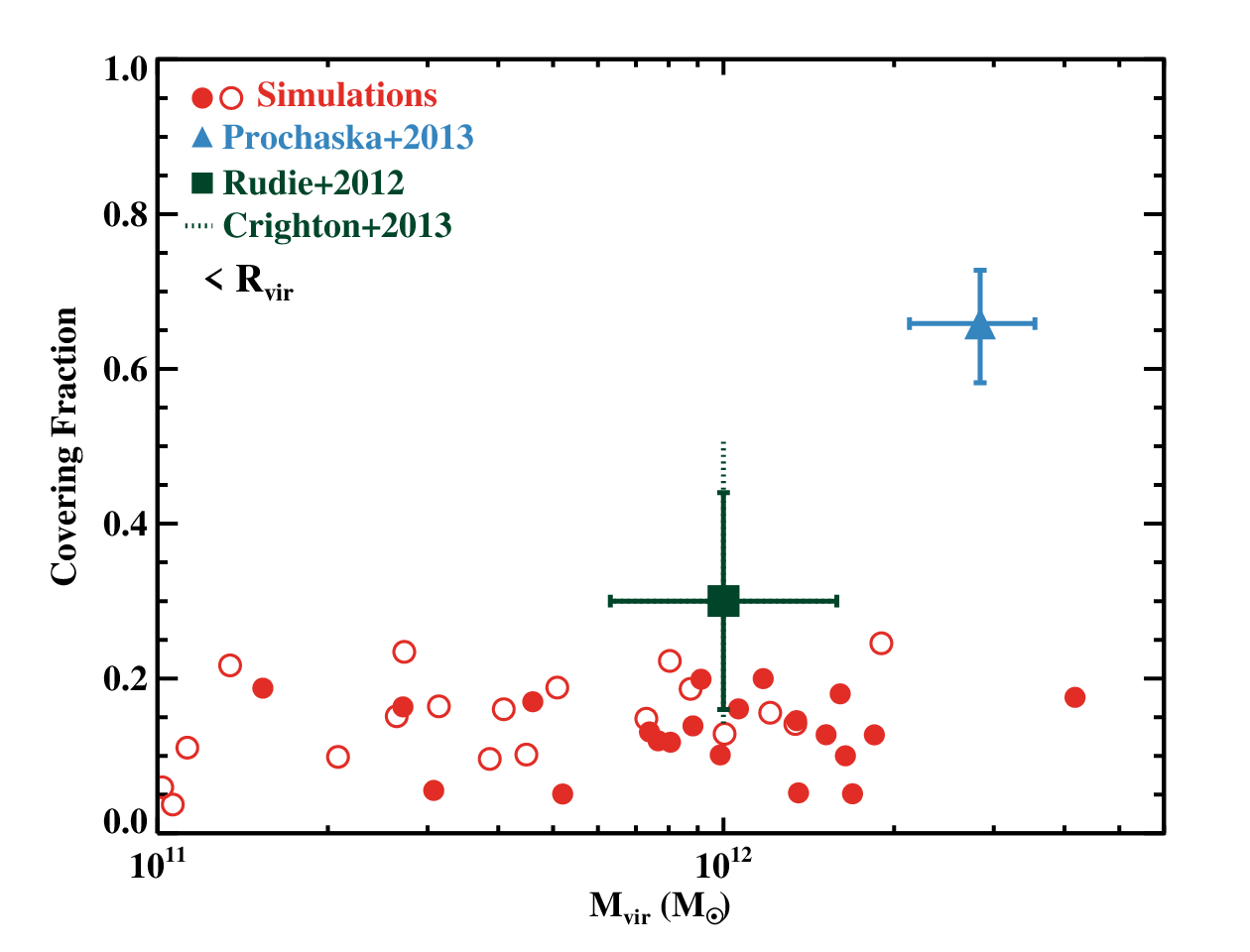
In Figure 4, we show again the simulated covering fractions within both at and , but we now superimpose measurements of the covering fractions of optically-thick gas for LBGs [97, N. Crighton et al., in prep.] and in quasar host galaxies [85].
Rudie et al. [97] have measured the covering fraction of optically-thick gas in a sample of 10 LBGs within 100 kpc from a bright background quasar. Typical halo masses for LBGs are inferred by comparing the observed clustering of galaxies to the clustering of dark matter halos in numerical simulations. In the following, we assume the mass interval of at from Adelberger et al. [1] [21, see also], where the uncertainty in the halo mass reflects the errors on the measured correlation function. However, different determinations may suffer from larger systematic uncertainties [7, see e.g.]. Assuming for galaxies at this mass, Rudie et al. [97] find within 68% confidence interval inside the virial radius. A similar analysis by N. Crighton et al. (in prep.) yields a comparable covering fraction, with slightly larger error bars.
A subset of our simulated galaxies or the Eris simulation by Shen et al. [101] approach the observed value. However, we emphasize that this comparison is subject to the uncertainties of the subgrid physics included in these simulations (see Section IV.3). As a population, the covering fraction in simulations () is a factor of 2 lower than what suggested by observations [97, cf.], but is nevertheless consistent given the large error bars. The mean covering fraction in simulations is in fact in formal agreement with observations, lying within the 68% confidence interval. This comparison therefore highlights how current samples of LBGs at in proximity to background quasars are too small to conclusively establish whether there is inconsistency between simulations and observations, limiting our ability to robustly test current theories for gas accretion onto galaxies.
The situation is instead different at larger masses, as shown in Figure 4. Using a sample of 74 quasar pairs, Prochaska et al. [85] have measured the covering fractions of optically-thick gas in the surroundings of quasar host galaxies at projected separations ranging from 30 to 300 kpc. Assuming a typical halo mass of for the quasar host halos deduced from the clustering measurements of [119], and a corresponding virial radius of , 27 optically-thick systems are found along the 41 sightlines that sample the halos within . The inferred covering fraction is therefore (68% confidence interval). As evident from Figure 4, this covering fraction significantly exceeds the values measured in these simulations.

IV.2. The radial dependence of
The Prochaska et al. [85] quasar pair sample is sufficiently large to enable measurements of the covering fraction as a function of projected separation from the foreground quasar. A comparison between observations and simulations for the 5 most massive halos above in our sample (MW12, SFG1, SFG7, SFG9, and VL11) is presented in Figure 5. The mean virial mass in this subset is (median ), comparable to the typical halo mass of quasar host galaxies. In this figure, the covering fractions and the corresponding 68% Wilson confidence intervals deduced from the observations are shown in bins of projected separation between the foreground quasar and the background quasar sightline. We have assumed the quasar resides at the center of its host dark matter halo. For a consistent comparison, we generated 1000 realizations of the same experiment conducted by Prochaska et al. [85], but using our simulations. For each trial, we randomly sample the five simulated halos along three orthogonal axis using 74 sightlines at the exact same set of impact parameters as the observed quasar pair sample.
The mean of the covering fractions computed for each bin are compared to the measurements in Figure 5, where we also show the standard deviation of the distribution of covering fraction in each bin measured from our ensemble of realizations. Because of the limited size of our simulation cube (4 on a side), the bin at the largest impact parameters is slightly undersampled in our mock observations (see bottom panel of Figure 5). The inconsistency between observations and simulations is readily apparent for separations . Given the limited number of sightlines within 50 kpc, the large difference between the observed and simulated covering fractions in the innermost bin is not statistically significant. However, in the interval between , all the simulated covering fractions are significantly below the observations, lying outside the 95% confidence interval measured for the quasar pair data. This striking discrepancy is also evident from the fact that there were 37 optically-thick systems found in the 74 observed sightlines, whereas we never found 37 or more such absorbers in our 1000 trials sampled at the same 74 impact parameters.
The picture that clearly emerges from this comparison is that the basic cosmological processes responsible for the assembly of massive galaxies, and particularly gas inflows, do not produce a sufficiently high covering fraction of optically-thick gas to explain the high value observed around quasar host galaxies. This is especially true given that our post processing radiative transfer does not include the effect of the additional ionizing photons from the quasar itself, which would even further reduce the covering fractions deduced from the simulations [50, 52, 85].
IV.3. Impact of feedback mechanisms on comparisons between simulations and observations
The foregoing analysis reveals that our understanding of the gas distribution in the massive galaxies that host quasars is incomplete. In this section, we briefly speculate on possible causes for the discrepancy highlighted by our study, focusing first on feedback mechanisms.
The simulations included in this study (as other simulations discussed in the recent literature) are imperfect models of our Universe, particularly because of the weak or ad-hoc implementation of feedback. As discussed in Section II, the average mass loading factors of the winds in these simulations is low, at 0.5. Therefore, these simulations overestimate the amount of stars formed by by a factor of , and consequently underpredict the gas fractions within the galaxy disks. This fact may impact the simulated properties of the CGM in several ways.
For instance, strong outflows would prevent gas to be locked into stars at high redshift, and additional material may then available for later accretion [82, cf.]. At the same time, stronger outflows may interact with the accreting material shaping its structure [34, 84, see a discussion in]. Further, a stronger implementation of stellar feedback [109, 101, 15, see e.g.], or an additional form of feedback from the central AGN, may be the astrophysical process that is needed to boost the covering fractions of optically-thick gas in these simulations. Besides alleviating or even resolving the tension between observations and simulations, feedback processes may also be required to reproduce the large equivalent widths of metal lines (e.g. for C II) that have been found within the virial radius of quasar host galaxies [85].
However, detailed absorption line modeling and analysis of the physical properties of a single quasar absorption system in Prochaska & Hennawi [88] indicated that the enriched gas detected in the quasar CGM was unlikely to represent material ejected from the AGN. Furthermore, as shown by van de Voort et al. [113] and Shen et al. [101], the majority of the cross section of optically-thick hydrogen lies in cold filaments, with only a small contribution originating in cold gas entrained within outflows. For these reasons, stronger feedback implementations that generate mostly hot winds may not significantly boost the cross section of optically-thick gas. Different implementations in which a larger fraction of cold material is entrained in the outflowing gas may be required to increase the cross section of optically-thick gas. Unfortunately, most of the relevant astrophysical and hydrodynamic processes that occur in winds are currently not fully resolved by cosmological hydrodynamic simulations [84, 62, 55, 24, see].
We also emphasize that resolution may play a significant role in shaping the structure of optically-thick gas in simulations, regardless to the adopted feedback models. At progressively lower resolution, high density peaks are smoothed out, and thus structures of size comparable to the grid cells are not properly capture in these simulations. Thus resolution may affect the resulting covering fraction directly, e.g. we could be missing small clumps of optically-thick gas, or indirectly, e.g. by altering the structure of the medium through which ionizing photons propagate during our radiative transfer post-processing.
IV.4. Additional causes for the discrepancies between simulations and observations
Besides incomplete physics in our simulations, other reasons can be invoked to account for the current inconsistency between simulations and observations at the high-mass end. Because of our limited simulation volume, the optically-thick gas modeled in these simulations resides within from the center of the halo. Conversely, the Prochaska et al. [85] analysis considered a velocity interval of , which was required because of significant uncertainties in the quasar redshifts [94]. This velocity interval corresponds to along the line-of-sight, and thus optically-thick systems detected at small projected distances (e.g. within ) from a foreground quasar could in fact lie at larger line-of-sight separations, and hence larger physical separations than we have considered.
Given the observed number of LLS per unit redshift at [80], the probability to intercept a random LLS from the cosmic background over such a small redshift path is however negligible compared to the large covering factors observed. However, if quasars reside at the center of larger scale structures, such as group of galaxies, which are each surrounded by optically-thick halo gas, then the observed covering factor may include a contribution from optically-thick absorbers at distances larger than the that we have considered. This effect needs to be investigated with simulations of larger cosmological volumes. However, we speculate that absorbers distance larger than can ease but not resolve the discrepancy between observations and simulations. Indeed, Prochaska et al. [85] measure a dropoff of the with impact parameter for (Figure 5), which suggests that optically-thick gas is mostly contained in proximity to the central galaxy and argues against a large contribution to the covering fraction from Mpc scales.
Finally, if quasars mark a particular phase in the life of a galaxy in which the AGN activity is triggered by mergers [98, 30, 56, e.g.], the observations of quasar pairs may provide only a biased view of the halo gas in massive galaxies. However, processes other than major mergers may be responsible for feeding AGNs, in particular at high redshifts [26, 19, 12, 20, 31, e.g.]. Furthermore, at the typical bolometric luminosity of the quasar pairs (), observations implies a star formation rate of [112, e.g.] which is comparable to the star formation rates observed in matched populations of non-active star forming galaxies [102, 99, 76, 47, 95, e.g.]. Thus, at present, there is no clear indication that quasar pairs reside in a population of halos that are systematically different than those described by our simulations.
V. A statistical view of the circumgalactic medium
As shown in Section IV, samples of LBG-quasar pairs are currently too limited in size for conclusive comparisons with simulations. In the second part of this paper, we therefore introduce the formalism for measuring the auto-correlation function of LLSs (Section V.2), which is based on an extension of the formalism used to measure the galaxy-LLS cross-correlation function (reviewed in Section V.1). The advantage of this experiment is to exploit larger samples of quasar pairs to statistically map the distribution of optically-thick hydrogen around galaxies at , avoiding the telescope-intensive task of finding many galaxy-quasar pairs.
V.1. The galaxy-LLS correlation function
In Figure 5, we have shown the radial dependence of the covering fraction in quasar host galaxies. This quantity, which is particularly useful to investigate the spatial extent of the CGM around galaxies of a given halo mass, can be recast in terms of the galaxy-LLS cross-correlation function [52, 86, see]. The cross-correlation function contains the same information as the covering fraction, but it has the advantage of directly comparing gas around galaxies to the cosmic background abundance of optically-thick hydrogen absorbers that are intercepted randomly as intervening LLSs. Thus, it directly quantifies the spatial scales for which a statistically significant excess of optically-thick absorption is detected around galaxies.
This cross-correlation function can also be compared to, e.g. the auto-correlation function of the galaxies themselves as well as the underlying dark-matter distribution, to help further constrain the distribution of CGM gas relative to the large-scale structure [100, 117, 23, e.g.]. Indeed, cross-correlation functions between galaxies and absorbers have already been studied in the literature. For instance, Bouché & Lowenthal [11] and Cooke et al. [22] measured the correlation between LBGs and damped Lyman- systems, while Hennawi & Prochaska [52], Font-Ribera et al. [37], and Prochaska et al. [86] measured the clustering of either LLSs or the Lyman- forest around quasars. Also, Tinker & Chen [110], Wild et al. [120], and Adelberger et al. [2] studied the correlation between galaxies or quasars and metal absorption lines.
With the exception of Hennawi & Prochaska [52] and Prochaska et al. [86], all previous work has measured clustering on scales larger than , and these larger scale clustering measurements constrain the dark matter halos hosting absorbers [110]. However, as we will argue below, the small-scale clustering (i.e. scales comparable to the virial radius) or “one-halo” term has the potential to provide a very sensitive test for simulations of the CGM around galaxies. In what follows, we briefly review the formalism to compute the galaxy-LLS correlation function, closely following the discussion in Hennawi & Prochaska [52]. We then show predictions of computed from numerical models which we will then compared to measurement for the LLS auto-correlation function.
V.1.1 Formalism
For a given a population of galaxies with redshifts that are probed by background quasars at projected separations , we describe the distribution of optically-thick gas around halos as an excess probability of finding a LLS in comparison to random expectation inside a velocity interval that is centered at the galaxy systemic redshift.
The probability of finding a LLS at random in the corresponding redshift interval is , where is the number of LLSs per unit redshift evaluated at . This probability, which is independent of the projected separation, expresses the covering fraction of absorbers from the cosmic background population of random intervening LLSs. At a distance from a foreground galaxy (or quasar host galaxy), the probability of intercepting optically-thick gas is enhanced by clustering around the galaxy according to
| (1) |
Here, is the projected galaxy-LLS cross-correlation function, which quantifies the excess probability above the cosmic mean of detecting LLSs near the galaxy in the corresponding redshift interval. As we will show below, this probability is directly related to the covering fraction of optically-thick gas around galaxies.
The projected correlation function can be related to the real-space galaxy-LLS correlation function with an average over the volume . Here,
| (2) |
in a flat cosmology, and is the cross section of the absorbing clouds. Under the assumption that ,
| (3) |
For an ensemble of galaxy/quasar pairs, the projected galaxy-LLS correlation function can be evaluated in bins11 1 For alternative method for computing the projected correlation function without binning data see, e.g., Hennawi & Prochaska [52]. of as
| (4) |
Here, is the number of LLSs detected around the galaxies in bins centered on and is the number of LLSs expected at random for a given . Given measurements of , one can determine the functional form for that best describes the observations using Equation (3).
V.1.2 Numerical models
Our goal is to show with simple numerical models how the LLS auto-correlation function can be used to gain insight into the properties of the CGM in comparison to the galaxy-LLS cross-correlation function, and not to produce detailed predictions for these two quantities. Therefore, we generate simple realizations of a universe in which LLSs are distributed around galaxies adopting the following prescriptions.
The spatial distribution of dark matter halos is given by the rockstar halo catalogue [6] extracted form the Bolshoi simulation [66], a dark matter only cosmological simulation in a box of 250 cMpc/h (comoving Mpc) on a side. We then model the spatial distribution of LLSs by populating dark matter halos at in the mass interval (consistent with the range explored in the previous sections) with a varying covering fraction of , and within 2. These values can be compared to the results of the hydrodynamic zoom-in simulations presented in the first part of this paper or to the observed values around LBGs [97].
In this way, we obtain realizations of a universe in which, by construction, a fraction of LLSs arise from halos in the specified mass interval, where is the volume density of dark matter halos in the selected mass range. To account for the remaining systems required to give the correct cosmic average line density of LLSs, i.e. , we simply add a random population of absorbers that are not clustered to dark matter halos and hence to galaxies. In all that follows, we take the incidence to be , which is consistent with the observed value for LLSs at from O’Meara et al. [80].
In other words, this model assumes a random, i.e. non-clustered, background of LLSs and of a second populations of LLSs that are clustered to galaxies in a selected mass range. Clearly, this is a rather simplistic approach as, for instance, simulations suggest that LLSs are typically clustered to galaxies of different masses [67, 4, 90, e.g.]. However, this approximation is meant to describe the limit in which a subset of LLSs arise from either low mass galaxies that have a small bias compared to the halos here considered, or to a case in which a fraction of LLS absorption arises along filaments in the intergalactic medium (IGM) and instead traces the Lyman- forest which has a very weak clustering compared to massive halos [74]. Albeit crude in its treatment of the baryon distribution around galaxies, this model accurately reproduces the spatial clustering on large scales that is imposed by structure formation.
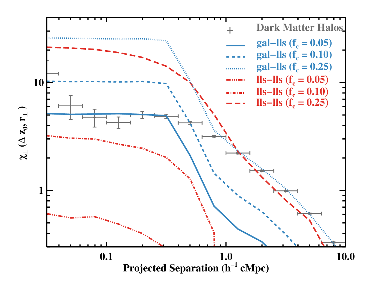
For the analysis, we sample these mock universes with random sightlines and we compute the projected galaxy-LLS cross-correlation function as described in Equation (4) within a velocity window of , corresponding to a redshift interval of or a depth of along the line of sight. This velocity window is suitable for comparisons with observations as it is large enough to encompass the majority of the denser gas () within 2 from the galaxy center, after accounting for peculiar velocities along the line of sight. Note that this velocity window is also larger than typical redshift errors for LBGs (). The resulting from the four different models with varying are shown in Figure 6 (blue lines) as a function of the projected separation between galaxies and LLSs. For comparison, we also show the projected two-point correlation function of dark matter halos (grey crosses), which we compute by comparing the number of galaxy pairs at projected distance within the Bolshoi simulation to the number of random pairs22 2 The two-point correlation function for dark matter halos flattens at scales of because of halo exclusion effects for which two halos cannot occupy the same volume..
Figure 6 provides a schematic view of the CGM properties that can be extracted from the galaxy-LLS correlation function. First, one can see that at projected separations that are typical for the one-halo term (), the projected correlation function is proportional to the covering fraction of optically-thick gas inside the dark matter halos. By construction, our models do not incorporate any radial dependence for within . However, our zoom-in simulations exhibit only a shallow radial profile for the covering fraction (see e.g. Figure 5), and a modest radial dependence for the projected correlation function up to becomes a general prediction. If we adopted a power law form for the correlation function , and fitted only data interior to that are dominated by this flat one-halo term, we would infer a large correlation length or, equivalently, a shallow exponent . A quantitative comparison between the observed and predicted galaxy-LLS cross-correlation function offers therefore an additional test for theories of gas accretion around galaxies.
The second feature that is visible in Figure 6 is that, around , the projected cross-correlation function exhibits a break at the transition between the one-halo term and the two-halo term. This feature offers a natural way to define the typical extent of the CGM in the galaxy population under examination. Finally, at larger projected separations (), the two-halo term of the cross-correlation function traces the (halo mass dependent) two-point correlation function of the dark matter halos that host LLSs. For models with large covering fractions such that , the galaxy-LLS and halo correlation functions overlap, while for models with lower , the amplitude of the galaxy-LLS correlation function is suppressed compared to the halo correlation function due to the increasingly higher contribution from the background, which in this particular modelization is randomly distributed, and hence dilutes the clustering signal. Note however that the shape of the cross-correlation function is preserved for the case of a large random background.
Finally, Figure 6 reveals that even models with modest covering fraction of optically-thick gas as predicted by our zoom-in simulations exhibit a high amplitude for the projected correlation function. This is a direct consequence of the limited number of LLSs that are expected at random within a velocity window of from a galaxy. Given the amplitude of the correlation function, for models with , samples of galaxies-quasar pairs are needed to detect the one-halo term of the galaxy-LLS correlation function at . To place interesting constraints on models, samples with at least 80 galaxy-LLS sightlines are needed. Twice as much pairs are instead required for this measurement for the case. The galaxy-LLS cross-correlation function has already been measured on small scales for the quasar host galaxies [52, 86]. However, building up the required statistics to make a measurement of comparable precision of the LBG-LLS cross-correlation is a more challenging task. While one can attempt to detect a signal with current data, samples that are 5 to 10 times larger than what currently available are needed to precisely characterize the distribution of optically-thick gas around galaxies.
V.2. The LLS auto-correlation function
To circumvent the observational challenges of building up large foreground galaxy-background quasar samples, we propose that one measures the auto-correlation function of LLSs, using the large existing samples of close quasar pairs, with pairs currently known at [48, 51, 53]. Further, one can exploit samples of lensed quasars to extend this measurement to even smaller scales of [59, e.g.]. The key advantage of this technique is that LLSs are easy to identify even in modest signal-to-noise spectra, and hence large samples of LLS pairs can be assembled at .
The idea of the LLS auto-correlation function builds on previous work that has shown the power of correlating absorption systems along multiple quasar sightlines to reveal the spatial distribution of hydrogen or metals in the IGM [74, 73, 105, 38, e.g.]. We now generalize the formalism presented for the galaxy-LLS correlation function to the case of two intervening LLSs (i.e. systems that are not physically associated to the background quasars) in the foreground of quasar pairs with projected separation . Next, we will show using numerical models that the LLS auto-correlation function contains the same information about the CGM of galaxies as is encoded in the galaxy-LLS cross-correlation function. Thus, if LLSs are associated to galaxies, searches for LLSs in quasar pairs provide a powerful statistical way to characterize the CGM in high redshift galaxies, without the need to identify individual galaxy-LLS associations.
V.2.1 Formalism
The formalism to compute the LLS auto-correlation function closely follows the approach used to compute the galaxy-LLS cross-correlation function. For a random quasar sightline, the probability to find a LLS is , where is the useful redshift path that can be searched for absorption lines. Once a LLS is found at redshift the probability of finding a second LLS within from the redshift of the first LLS along a second sightline at distance is
| (5) |
where and expresses the projected LLS auto-correlation function. As we will show in the following, if LLSs mostly arise from galaxy halos, is directly related to the covering fraction of optically-thick gas in the CGM in the galaxy population from which LLSs arise.
As previously done for the galaxy-LLS correlation function, we can relate to the LLS auto-correlation function in real space following Equation (3). Altogether, assuming , the probability to find a pair of LLSs in the foreground of a quasar pair becomes
| (6) |
For an ensemble of quasar pairs, one can measure the projected LLS auto-correlation function in bins of following Equation 4.
V.2.2 Numerical models
Provided that the population of LLSs can be identified with the CGM of galaxies [67, 39, 113, 40], a LLS detected at redshift along one sightline signals the presence of a galaxy, which lie at an unknown projected distance . Therefore, even without identifying the galaxies that are responsible for the absorption, one can use a second sightline at projected separation from the first quasar to probe the distribution of optically-thick gas in the galaxy halo. The LLS auto-correlation function is thus analogous to the galaxy-LLS correlation function, providing a statistical way of mapping the CGM of distant halos without explicitly identifying galaxy-LLS associations.
To illustrate this point with numerical models, we generate a new realization from the Bolshoi simulation assuming , such that the majority of LLSs arise from halos with masses . We then sample the simulated box with pairs of sightlines with separations and compute the projected LLS auto-correlation function as described in Equation (4), that is by comparing the pairs of LLSs with a given and within a velocity window of to the random expectation. The resulting LLS auto-correlation function is shown with a red dashed line in Figure 6. Note that in this figure the projected separation on the x-axis corresponds to the distance between quasar pairs for the LLS auto-correlation function, while it corresponds to the separation between a quasar sightline and a galaxy (assumed to be at the center of the dark matter halo in our models) for the galaxy-LLS correlation function.
As is evident from Figure 6, the projected LLS auto-correlation function closely resembles the projected galaxy-LLS correlation function for . The only difference is that for the galaxy-LLS pairs, the galaxy is always at the center of the dark matter halo, whereas for the LLS-LLS pairs, the halo centers are offset by a random amount relative to the two quasars probing the LLSs, and thus reflects the properties of the halo gas smoothed on scales that are comparable to the size of the CGM, or in our numerical models. Nevertheless, the LLS auto-correlation function encodes all the information we previously discussed for the galaxy-LLS correlation function. This includes a flat one-halo term with an amplitude that varies with the covering fraction in the host halos, a one-halo to two-halo term transition that can be used to define the characteristic size of the CGM in the galaxies where LLSs arise, and a two-halo term which traces the large-scale clustering of the underlying dark matter halos hosting LLSs. The fact that the large scale LLS correlation traces the clustering of dark matter halos is a trivial consequence of how we constructed our models by associating LLSs only to dark matter halos in a selected mass range. However, this exercise shows how measurements of the large-scale LLS auto-correlation function can be used to determine the typical halo masses which host LLSs, a key unknown quantity that currently hampers the interpretation of the observed LLS properties [40, e.g.].
In Figure 6, we also show the LLS auto-correlation function in a realization with (red dotted line) and (red dashed triple-dotted line). In the latter case, the majority of LLSs () are not clustered to galaxies, but they reside in a random background. As expected, one can see how the projected auto-correlation function approaches zero. A comparison between the three models with is useful to highlight the two extreme behaviors that the LLS auto-correlation function may reflect. For high covering fractions, or more generally when the product of the covering fraction and the size of the CGM is large (as suggested by current observations), the number of LLSs that are associated to galaxies exceeds the number of LLSs in a random (non clustered) background. In this case, and thus the LLS auto-correlation function yields information on the CGM properties. Conversely, if either is small or the radial profile of optically-thick gas in the CGM is very steep, then the number of LLSs associated to galaxies is much smaller than the number of LLSs in a random background and . In this case, a measurement of the LLS auto-correlation function can be used to conclude that LLSs are not associated to massive galaxies, but rather they originate from a more weakly clustered population, e.g. the Lyman- forest. It should also be noted that if the fraction of LLSs that are associated to galaxies evolves with redshift [40, cf.], then the auto-correlation function of LLSs will evolve accordingly.
From the above discussion, it follows the LLS auto-correlation function encodes information on the cross section of optically thick gas around galaxies, similarly to the measurement of the cross-correlation function of damped Lyman- systems with the Lyman- forest [38, see]. For instance, in constructing these simple models, we have assume a mass-independent covering fraction within 2, which implies a mass dependent cross section . In computing the LLS auto-correlation function, determines the weight with which each halo of a given mass contributes to the observed value of . For this reason, a precise measurement of the auto-correlation of optically-thick systems around quasar pairs provides a way to constrain the mass-dependent cross section , a quantity for which theoretical predictions exist from hydrodynamic simulations [9, e.g.].
We conclude by noting that, thanks to the large samples of quasar spectra that currently are or will be soon available from surveys like the Sloan Digital Sky Survey [83, SDSS; e.g.], a measurement of the LLS auto-correlation function can be obtained at large scales () at redshifts . The minimum angular separation is set by the fiber collision limit in the spectroscopic survey, which severely limits the number of close quasar pairs with available spectroscopy, while the redshift constraint is currently set by the throughput of the survey spectrograph. However, because of the SDSS color-selection bias that preferentially selects quasars with LLS absorption at [121, 40], additional investigation is needed to establish whether the redshift limit has to be restricted to .
To measure the LLS auto-correlation function on small scales, hundreds of spectroscopically confirmed quasar pairs with projected separations between have now been discovered via follow-up spectroscopy of the SDSS imaging [48, 51, 53]. This sample allows a precise measurement of the small-scale clustering at high confidence level ( for ). Although the majority of useful pairs are currently between requiring the use of space-based facilities to identify LLSs in the foreground of these quasar pairs, a precise measurement of the LLS auto-correlation function on all scales can potentially be achieved in the near future.
VI. Summary and conclusions
We have analyzed the hydrogen distribution in the surroundings of 21 galaxies at that have been simulated at high resolution with virial masses . After post-processing these simulations with a Monte Carlo radiative transfer code to identify regions that retain enough neutral hydrogen to remain optically thick to Lyman continuum radiation, we have directly compared the covering fraction of optically-thick gas in simulations and observations of LBGs and quasar host galaxies. We have also presented a formalism to compute the galaxy-LLS cross-correlation function and the LLS auto-correlation function, and we have provided simple estimates for these quantities using numerical simulations. Our main findings can be summarized as follows.
The covering fractions of optically-thick gas within the virial radius of the simulated galaxies range between , where the large scatter is driven by intrinsic variation in the gas distributions around individual halos. Within 2, we have found instead , implying that the area subtended by optically-thick gas within and between is approximately the same. While our simulations exhibit the expected increase in the average gas temperature and an increase in the mass fraction of hot gas above virial masses for which stable virial shocks form, we have found that the mass fraction of cold gas with is only weakly dependent on halo mass. Further, at , we have not found any strong dependence of the covering fraction on the halo mass, even beyond the critical mass for the formation of virial shocks.
Once compared to observations of 10 galaxy-quasar pairs at , these simulations are statistically consistent with the observed covering fraction of optically-thick gas inside the virial radius. However, current samples are too small to make a conclusive comparison, preventing stringent tests for current theories of cold gas accretion. Conversely, simulated halos at exhibit covering fractions at all radii that significantly underestimate the values observed in the surroundings of quasar host galaxies. This discrepancy reveals that our numerical models do not fully capture all of the physical processes necessary to describe the gas distribution around massive halos. At present, we do not know the explanation for this disagreement, but issues that should be investigrated in future work are i) modeling the effects of stronger (AGN) feedback and/or small-scales hydrodynamic instabilities than what is currently implemented in our simulations, ii) or a better understanding on how the properties of quasar host galaxies, in particular their star-formation rates or gas masses, compare to other populations of star-forming galaxies such as the LBGs.
Further, we have showed how mesurements of the galaxy-LLS correlation function can be used to measure the ccovering fraction of LLSs around galaxies. The flat radial depence of the covering fraction interior to the predicted by our simulations, implies that the projected galaxy-LLS correlation function will exhibit a shallow radial dependence on small-scales that probe the one-halo term. We have also showed that the transition between the one-halo term and two-halo term imprints a feature in the projected cross-correlation function that can be used to define the spatial extent of the CGM.
Finally, under the assumption that LLSs are statistically associated to galaxy halos of a given mass range, we have proposed a measurement of the LLS auto-correlation function using quasar pair sightlines, to map the spatial distribution of optically-thick gas around galaxies, without the need to identify individual galaxy-LLS associations. Our numerical models show that the LLS auto-correlation function encodes the same information contained in the galaxy-LLS correlation function (both covering fraction of optically-thick gas, the characteristic size for the CGM), but smoothed on scales comparable to the typical size of the CGM. Furthermore, we have highlighted that at large separations the two-halo term of the LLS auto-correlation function traces the two-point correlation function of the dark matter halos hosting LLSs, providing long-sought information about the typical mass of the halos that host LLSs.
While our analysis underscores a still incomplete view of the gas distribution around massive galaxies, in this paper we have outlined a possible path towards an improved knowledge of the properties of the halo gas in the distant Universe. In the long term, the increasing availability of samples of quasar-galaxy pairs will offer a direct way to map the radial distribution of optically-thick gas at high redshift. Measurements of the galaxy-LLS correlation can be compared to different sets of simulations, providing additional insights into the processes that regulate the structure of the CGM and ultimately the formation and evolution of galaxies. Given the current availability of large spectroscopic samples of quasars and hundreds of quasar pairs with small projected separations, it is also possible to compute the LLS auto-correlation function to obtain the first view of the spatial distribution of optically-thick gas in the high-redshift Universe.
As discussed, this measurement would provide an important test for the cold-stream paradigm, as well as a solid empirical assessment of whether LLSs arise primarily in the CGM of galaxies at . Provided that the connection between LLSs and halo gas can be robustly established, analysis of the physical properties of these absorbers would then offer a powerful way to map the metal distribution in proximity to galaxies in the distant Universe. Further, better knowledge on the clustering of LLSs would affect estimates for the extragalactic UV background, that depend strongly on the distribution of optically-thick gas. It is therefore clear that an improved understanding of how LLSs cluster around galaxies and around themselves would constitute an important step forward that will impact several areas of study.
References
- [1] Adelberger, K. L., Steidel, C. C., Pettini, M., et al. 2005, ApJ, 619, 697
- [2] Adelberger, K. L., Shapley, A. E., Steidel, C. C., et al. 2005, ApJ, 629, 636
- [3] Agertz, O., Moore, B., Stadel, J., et al. 2007, MNRAS, 380, 963
- [4] Altay, G., Theuns, T., Schaye, J., Crighton, N. H. M., & Dalla Vecchia, C. 2011, ApJ, 737, L37
- [5] Bauer, A., & Springel, V. 2012, MNRAS, 423, 2558
- [6] Behroozi, P. S., Wechsler, R. H., Wu, H.-Y., et al. 2013, ApJ, 763, 18
- [7] Bielby, R., Hill, M. D., Shanks, T., et al. 2013, MNRAS, 430, 425
- [8] Binney, J. 1977, ApJ, 215, 483
- [9] Bird, S., Vogelsberger, M., Sijacki, D., et al. 2013, MNRAS, 429, 3341
- [10] Birnboim, Y., & Dekel, A. 2003, MNRAS, 345, 349
- [11] Bouché, N., & Lowenthal, J. D. 2004, ApJ, 609, 513
- [12] Bournaud, F., Dekel, A., Teyssier, R., et al. 2011, ApJ, 741, L33
- [13] Cantalupo, S., Lilly, S. J., & Haehnelt, M. G. 2012, MNRAS, 425, 1992
- [14] Cantalupo, S., & Porciani, C. 2011, MNRAS, 411, 1678
- [15] Ceverino, D., Klypin, A., Klimek, E., et al. 2013, arXiv:1307.0943
- [16] Ceverino, D., & Klypin, A. 2009, ApJ, 695, 292
- [17] Ceverino, D., Dekel, A., Mandelker, N., et al. 2012, MNRAS, 420, 3490
- [18] Ceverino, D., Dekel, A., & Bournaud, F. 2010, MNRAS, 404, 2151
- [19] Ciotti, L., Ostriker, J. P., & Proga, D. 2010, ApJ, 717, 708
- [20] Cisternas, M., Jahnke, K., Bongiorno, A., et al. 2011, ApJ, 741, L11
- [21] Conroy, C., Shapley, A. E., Tinker, J. L., Santos, M. R., & Lemson, G. 2008, ApJ, 679, 1192
- [22] Cooke, J., Wolfe, A. M., Gawiser, E., & Prochaska, J. X. 2006, ApJ, 652, 994
- [23] Cooray, A., & Sheth, R. 2002, Phys. Rep., 372, 1
- [24] Creasey, P., Theuns, T., & Bower, R. G. 2013, MNRAS, 429, 1922
- [25] Crighton, N. H. M., Bielby, R., Shanks, T., et al. 2011, MNRAS, 414, 28
- [26] Davies, R. I., Maciejewski, W., Hicks, E. K. S., et al. 2009, ApJ, 702, 114
- [27] Dekel, A., Zolotov, A., Tweed, D., et al. 2013, arXiv:1303.3009
- [28] Dekel, A., et al. 2009, Nature, 457, 451
- [29] Dekel, A., & Birnboim, Y. 2006, MNRAS, 368, 2
- [30] Di Matteo, T., Springel, V., & Hernquist, L. 2005, Nature, 433, 604
- [31] Di Matteo, T., Khandai, N., DeGraf, C., et al. 2012, ApJ, 745, L29
- [32] Dijkstra, M., & Loeb, A. 2009, MNRAS, 400, 1109
- [33] Fardal, M. A., Katz, N., Gardner, J. P., Hernquist, L., Weinberg, D. H., & Davé, R. 2001, ApJ, 562, 605
- [34] Faucher-Giguère, C.-A., Kereš, D., & Ma, C.-P. 2011, MNRAS, 417, 2982
- [35] Faucher-Giguère, C.-A., & Kereš, D. 2011, MNRAS, 412, L118
- [36] Faucher-Giguère, C.-A., Kereš, D., Dijkstra, M., Hernquist, L., & Zaldarriaga, M. 2010, ApJ, 725, 633
- [37] Font-Ribera, A., Arnau, E., Miralda-Escudé, J., et al. 2013, JCAP, 5, 18
- [38] Font-Ribera, A., Miralda-Escudé, J., Arnau, E., et al. 2012, JCAP, 11, 59
- [39] Fumagalli, M., Prochaska, J. X., Kasen, D., et al. 2011, MNRAS, 418, 1796
- [40] Fumagalli, M., O’Meara, J. M., Prochaska, J. X., & Worseck, G. 2013, ApJ, 775, 78
- [41] Furlanetto, S. R., Schaye, J., Springel, V., & Hernquist, L. 2005, ApJ, 622, 7
- [42] Genzel, R., Burkert, A., Bouché, N., et al. 2008, ApJ, 687, 59
- [43] Goerdt, T., Dekel, A., Sternberg, A., Gnat, O., & Ceverino, D. 2012, MNRAS, 424, 2292
- [44] Goerdt, T., Dekel, A., Sternberg, A., Ceverino, D., Teyssier, R., & Primack, J. R. 2010, MNRAS, 407, 613
- [45] Haardt, F., & Madau, P. 2012, ApJ, 746, 125
- [46] Haiman, Z., Spaans, M., & Quataert, E. 2000, ApJ, 537, L5
- [47] Harrison, C. M., Alexander, D. M., Mullaney, J. R., et al. 2012, ApJ, 760, L15
- [48] Hennawi, J. F. 2004, Ph.D. Thesis
- [49] Hennawi, J. F., & Prochaska, J. X. 2013, ApJ, 766, 58
- [50] Hennawi, J. F., Prochaska, J. X., Burles, S., et al. 2006, ApJ, 651, 61
- [51] Hennawi, J. F., Strauss, M. A., Oguri, M., et al. 2006, AJ, 131, 1
- [52] Hennawi, J. F., & Prochaska, J. X. 2007, ApJ, 655, 735
- [53] Hennawi, J. F., Myers, A. D., Shen, Y., et al. 2010, ApJ, 719, 1672
- [54] Hopkins, P. F. 2013, MNRAS, 428, 2840
- [55] Hopkins, P. F., Quataert, E., & Murray, N. 2012, MNRAS, 421, 3522
- [56] Hopkins, P. F., Hernquist, L., Cox, T. J., et al. 2005, ApJ, 630, 705
- [57] Hummels, C. B., Bryan, G. L., Smith, B. D., & Turk, M. J. 2013, MNRAS, 430, 1548
- [58] Iliev, I. T., Ciardi, B., Alvarez, M. A., et al. 2006, MNRAS, 371, 1057
- [59] Inada, N., Oguri, M., Shin, M.-S., et al. 2012, AJ, 143, 119
- [60] Kasen, D., Thomas, R. C., & Nugent, P. 2006, ApJ, 651, 366
- [61] Jefferies, J. T. 1968, A Blaisdell Book in the Pure and Applied Sciences, Waltham, Mass.: Blaisdell, 1968
- [62] Joung, M. R., Bryan, G. L., & Putman, M. E. 2012, ApJ, 745, 148
- [63] Kennicutt, R. C., Jr. 1998, ApJ, 498, 541
- [64] Kereš, D., Katz, N., Weinberg, D. H., & Davé, R. 2005, MNRAS, 363, 2
- [65] Kereš, D., Katz, N., Fardal, M., Davé, R., & Weinberg, D. H. 2009, MNRAS, 395, 160
- [66] Klypin, A. A., Trujillo-Gomez, S., & Primack, J. 2011, ApJ, 740, 102
- [67] Kohler, K., & Gnedin, N. Y. 2007, ApJ, 655, 685
- [68] Komatsu, E., et al. 2009, ApJS, 180, 330
- [69] Kravtsov, A. V., Klypin, A. A., & Khokhlov, A. M. 1997, ApJS, 111, 73
- [70] Kravtsov, A. V. 2003, ApJ, 590, L1
- [71] Kroupa, P. 2001, MNRAS, 322, 231
- [72] Lucy, L. B. 2002, A&A, 384, 725
- [73] Martin, C. L., Scannapieco, E., Ellison, S. L., et al. 2010, ApJ, 721, 174
- [74] McDonald, P. 2003, ApJ, 585, 34
- [75] Miller, G. E., & Scalo, J. M. 1979, ApJS, 41, 513
- [76] Mullaney, J. R., Pannella, M., Daddi, E., et al. 2012, MNRAS, 419, 95
- [77] Nelson, D., Vogelsberger, M., Genel, S., et al. 2013, MNRAS, 429, 3353
- [78] Nestor, D. B., Shapley, A. E., Kornei, K. A., Steidel, C. C., & Siana, B. 2013, ApJ, 765, 47
- [79] Ocvirk, P., Pichon, C., & Teyssier, R. 2008, MNRAS, 390, 1326
- [80] O’Meara, J. M., Prochaska, J. X., Worseck, G., Chen, H.-W., & Madau, P. 2013, ApJ, 765, 137
- [81] Oppenheimer, B. D., & Schaye, J. 2013, arXiv:1302.5710
- [82] Oppenheimer, B. D., Davé, R., Kereš, D., et al. 2010, MNRAS, 406, 2325
- [83] Pâris, I., Petitjean, P., Aubourg, É., et al. 2012, A&A, 548, A66
- [84] Powell, L. C., Slyz, A., & Devriendt, J. 2011, MNRAS, 414, 3671
- [85] Prochaska, J. X., Hennawi, J. F., Simcoe, R. 2013, ApJ, 762, 19
- [86] Prochaska, J. X., Hennawi, J. F., Lee, K.-G., et al. 2013, arXiv:1308.6222
- [87] Prochaska, J. X., O’Meara, J. M., & Worseck, G. 2010, ApJ, 718, 392
- [88] Prochaska, J. X., & Hennawi, J. F. 2009, ApJ, 690, 1558
- [89] Rahmati, A., Pawlik, A. H., Raičevic, M., & Schaye, J. 2013, MNRAS, 430, 2427
- [90] Rahmati, A., Schaye, J., Pawlik, A. H., & Raičevic, M. 2013, MNRAS, 989
- [91] Rauch, M., Becker, G. D., Haehnelt, M. G., Gauthier, J.-R., & Sargent, W. L. W. 2013, MNRAS, 429, 429
- [92] Read, J. I., & Hayfield, T. 2012, MNRAS, 422, 3037
- [93] Rees, M. J., & Ostriker, J. P. 1977, MNRAS, 179, 541
- [94] Richards, G. T., Vanden Berk, D. E., Reichard, T. A., et al. 2002, AJ, 124, 1
- [95] Rosario, D. J., Mozena, M., Wuyts, S., et al. 2013, ApJ, 763, 59
- [96] Rosdahl, J., & Blaizot, J. 2012, MNRAS, 423, 344
- [97] Rudie, G. C., Steidel, C. C., Trainor, R. F., et al. 2012, ApJ, 750, 67
- [98] Sanders, D. B., Soifer, B. T., Elias, J. H., et al. 1988, ApJ, 325, 74
- [99] Santini, P., Rosario, D. J., Shao, L., et al. 2012, A&A, 540, A109
- [100] Seljak, U. 2000, MNRAS, 318, 203
- [101] Shen, S., Madau, P., Guedes, J., et al. 2013, ApJ, 765, 89
- [102] Shao, L., Lutz, D., Nordon, R., et al. 2010, A&A, 518, L26
- [103] Silk, J. 1977, ApJ, 211, 638
- [104] Sijacki, D., Vogelsberger, M., Kereš, D., Springel, V., & Hernquist, L. 2012, MNRAS, 424, 2999
- [105] Slosar, A., Font-Ribera, A., Pieri, M. M., et al. 2011, Journal of Cosmology and Astroparticle Physics, 9, 1
- [106] Steidel, C. C., Erb, D. K., Shapley, A. E., Pettini, M., Reddy, N., Bogosavljević, M., Rudie, G. C., & Rakic, O. 2010, ApJ, 717, 289
- [107] Stewart, K. R., Kaufmann, T., Bullock, J. S., et al. 2011b, ApJ, 738, 39
- [108] Stewart, K. R., Kaufmann, T., Bullock, J. S., et al. 2011a, ApJ, 735, L1
- [109] Stinson, G. S., Brook, C., Prochaska, J. X., et al. 2012, MNRAS, 425, 1270
- [110] Tinker, J. L., & Chen, H.-W. 2008, ApJ, 679, 1218
- [111] Trainor, R. F., & Steidel, C. C. 2012, ApJ, 752, 39
- [112] Trakhtenbrot, B., & Netzer, H. 2010, MNRAS, 406, L35
- [113] van de Voort, F., Schaye, J., Altay, G., & Theuns, T. 2012, MNRAS, 421, 2809
- [114] van de Voort, F., Schaye, J., Booth, C. M., Haas, M. R., & Dalla Vecchia, C. 2011, MNRAS, 414, 2458
- [115] Verner, D. A., Ferland, G. J., Korista, K. T., & Yakovlev, D. G. 1996, ApJ, 465, 487
- [116] Verner, D. A., & Ferland, G. J. 1996, ApJS, 103, 467
- [117] Weinberg, D. H., Davé, R., Katz, N., & Hernquist, L. 2004, ApJ, 601, 1
- [118] White, S. D. M., & Rees, M. J. 1978, MNRAS, 183, 341
- [119] White, M., Myers, A. D., Ross, N. P., et al. 2012, arXiv:1203.5306
- [120] Wild, V., Kauffmann, G., White, S., et al. 2008, MNRAS, 388, 227
- [121] Worseck, G., & Prochaska, J. X. 2011, ApJ, 728, 23
- [122] Wood, K., & Loeb, A. 2000, ApJ, 545, 86
- [123] Woosley, S. E., & Weaver, T. A. 1995, ApJS, 101, 181
Appendix A Method for Calculating Ionizing Radiation Transport
To calculate the transport of ionizing radiation, we used a 3D Monte Carlo (MC) code, derived from the SEDONA code framework [60] and using an approach similar to that described in [122]. The radiation field is represented by a large number () of discrete photon packets, which are propagated throughout absorption or scattering events until they escape the simulation domain. This approach permits an arbitrary number of individual sources and conserves energy by construction. In addition, we are able to properly model the diffuse ionizing radiation field arising from recombinations to the ground state – i.e., we do not make the “on-the-spot” approximation. The main disadvantage of MC methods is that a large number of photon packets must be used to overcome statistical noise, however the method scales well and can be run on massively parallel machines.
The calculation in this paper ignores time-dependent effects and makes the assumption of ionization equilibrium [14, 81, cf.]. Each photon packet carries a “luminosity” of , where and are the total ionizing luminosities from the UVB and from local sources, respectively. A fraction of the photon packets are selected to represent the UVB. These packets are initially distributed randomly over the surface of a sphere of radius , chosen to be larger than the simulation box. The effective luminosity of the UVB from this outer surface is given by
| (A1) |
where we choose a UVB mean intensity at and (according to the redshift of each snapshot) from Haardt & Madau [45]. For simplicity, the spectrum of the UVB is assumed to be flat over the energy range Rydberg ( Å) corresponding to the wavelength region from the HeII ionization threshold to the hydrogen threshold.
To produce a homogenous UVB radiation field within the simulation domain, the directionality of the packets is sampled from a angular distribution, where is the angle between the packet direction vector and the inward local radial vector. To test the validity of this approach, we ran a calculation using packets and assuming that the opacity throughout the domain was zero everywhere. A nearly uniform UVB of the desired mean intensity was achieved in the simulation box, with random errors of the order of .
The remaining of the packets are selected to represent the ionizing radiation from local sources, and are emitted isotropically from locations given by the star particles from the hydrodynamic simulation. The probability of a packet being emitted from a given star particle is proportional to the UV luminosity of that star particle [39, see]. As with the UVB, the spectrum of local sources is assumed to be flat between 1 and 4 Rydberg.
Packets are propagated through the AMR grid until they are absorbed or escape the domain. The mean free path to a photoionization interaction with neutral hydrogen is given by where is the photoionization cross-section. Whenever a photon ionizes a hydrogen atom, the atom is assumed to recombine either to the ground state or to an excited state followed by a cascade to the ground state. The former case corresponds to an “effective scattering” in which an ionizing photon is immediately re-emitted in a new direction. The probability of this occurring is where is the recombination coefficient to the ground state while is the coefficient for recombination to all levels including the ground state. We assume a constant value appropriate for gas at K, as this quantity is only weakly dependent on temperature. At each ionization interaction event, a random number is chosen to determine whether recombination to the ground state occurs; if so, the photon packet is redirected isotropically, assigned a new wavelength from the local emissivity function, and its propagation continues until a true absorption occurs.
To calculate the state of the gas, ionization equilibrium is assumed,
| (A2) |
where and are, respectively, the hydrogen photoionization and collisional ionization rates, and is the hydrogen radiative recombination rate (all per cm3). At these low densities collisional recombination can be ignored. The photoionization rate is given by
| (A3) |
where is the total hydrogen density, is the fraction of hydrogen in the neutral state, and is the mean intensity of the ionizing radiation field. The radiative recombination rate is
| (A4) |
where is the proton density, and the electron density. For these calculations, we assume helium is neutral and does not contribute to the free electron density. In that case, we take . Expressions for and are taken from Verner et al. [115] and Verner & Ferland [116], respectively, and the collisional ionization rate from Jefferies [61].
During the MC procedure, an estimate of the photoionization rate (Equation (A3)) is constructed in each cell by tallying all traversing packets [72, 122, e.g.,]
| (A5) |
where is the cell volume, and the sum runs over all steps of length that occur for packets passing through the cell.
An iterative approach is used to converge the model to ionization equilibrium. Initially, a guess is made as to the neutral fraction in all cells. We then follow the MC transport and construct the estimator Equation (A5). By solving Equation (A2), we obtain a new value for the neutral fraction in each cell. The MC transport routine is then rerun, and a new estimate of is derived. This procedure is iterated until the ionization state no longer changes significantly from one iteration to the next. To speed convergence, we adopt as an initial guess that hydrogen is completely ionized everywhere, as in this case photons packets can propagate information across the entire domain. We find that 12 iterations are sufficient for convergence.
To validate the photoionization code, we perform test 1 of Iliev et al. [58] which consists of a box of dimension kpc with uniform gas number density . ú A source of ionizing photons with a production rate is placed at the center of the box. Figure 7 shows the resulting equilibrium ionization structure, which is in agreement with the converged structure presented in figure 8 of Iliev et al. [58].
