Calculation of Multipolar Exchange Interactions in Spin-Orbital Coupled Systems

Magnetic systems with strong spin-orbit coupling have been a theoretically challenging problem for decades due to their complex magnetic behavior and the lack of efficient computational techniques to solve model Hamiltonians describing them. They not only have active orbital degrees of freedom, which make these systems rich in magnetic properties, but they also possess a large number of parameters in the form of corresponding inter-site exchange interactions [1, 2, 3, 4, 5, 6, 7, 8, 9, 10, 11, 12]. In 60s, Schrieffer et. al. proposed a framework regarding the exchange interactions mediated by RKKY mechanism in such systems [1, 2, 3]. Unlike traditional spin $\frac{1}{2}$ problem where a simple Heisenberg model describes the low-energy physics well [22], the orbital degrees of freedom introduce more complicated multipolar exchange couplings, accompanied by large inter–site anisotropy, which makes the problem computationally difficult [12]. In 80s, Cooper et. al. solved the Coqblin–Schrieffer Hamiltonian for Cerium compounds and, in 90s, proposed a scheme to compute the exchange constants via advanced electronic calculations [4, 5, 6, 7, 8, 9, 10, 11]. Although their works are in good agreement with experiments for selected simple materials, an efficient and systematic method to calculate the exchange interaction is still lacking.

In this work, we introduce a new method combined with electronic structure calculations based on density functional theory (DFT) in its local density approximation (LDA) or including the correction due to Hubbard U via so–called LDA+U method [19], to compute the exchange interactions of systems with strong spin-orbit coupling (SOC). It is based on the theorem that multipolar tensor harmonics form a complete orthonormal basis set with respect to the trace inner product. Applying this theorem to the density matrix of the correlated magnetic orbital, well–defined scalar, dipole, quadrupole, and higher multipoles can be extracted [12]. By flipping a pair of tensor harmonics with respect to the ground–state density matrix, we can find the exchange interaction by relating (or mapping) it to the total energy cost of the tensor flip (which is obtained by the LDA+U calculation).

To test our new method, we use Uranium Dioxide (UO₂) as a test candidate due to the presence of dipolar and quadrupolar order in its ground state. UO₂ has been one of the widely discussed actinide compounds due to its applications in nuclear energy industry. It is a Mott insulator with cubic structure and well–localized $5f^{2}$ electrons (Uranium configuration U⁴⁺ by naive charge counting). Below $T_{N}=30.8K$ it undergoes a first–order magnetic and structural phase transition where a noncollinear antiferromagnetic (AFM) phase with tranverse 3-$\mathbf{k}$ magnetic ordering accompanied by the cooperative Jahn–Teller distortion occurs [14]. The two–electron ground state forms a $\Gamma_{5}$ triplet holding pseudospin $S=1$ rotation symmetry making it a good choice to test our method, as it is a minimal challenge beyond $S=\frac{1}{2}$ Heisenberg model. Description of a $S=1$ exchange interaction requires the existence of dipolar and quadrupolar moments, and it is commonly believed that there are two major mechanisms to induce exchange coupling: 1) superexchange (SE), and 2) spin–lattice interaction (SL). The former contributes to both dipole and quadrupole and the latter contributes to quadrupole only because of the symmetry of the distortion. The dominance of SE or SL in affecting the quadrupole exchange remains a controversial issue [13, 14, 15, 16]. Since our method is based on a static electronic calculation, we do not explore dynamical effects in all their details. Therefore, separate calculations using the coupled frozen–phonon and frozen–magnon techniques were performed to extract the SL coupling constants. Although we have chosen $UO_{2}$ as our test sample whose static exchange interactions originate from superexchange mechanism, it should be emphasized that our method should be able to work for any other types of exchange processes.

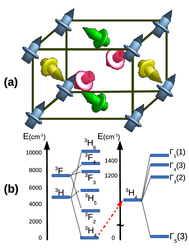
A non–hermitian unit spherical tensor operator is defined as: $Y_{K}^{Q}(J)=\sum_{MM^{\prime}}(-1)^{J-M}(2K+1)^{2}\times\left(\begin{smallmatrix}J&J&K\\ M^{{}^{\prime}}&-M&Q\end{smallmatrix}\right)|JM\rangle\langle JM^{{}^{\prime}}|$. We can further define hermitian cubic tensor harmonics $T_{K}^{Q}(J)=\frac{1}{\sqrt{2}}[(-1)^{Q}Y_{K}^{Q}(J)+Y_{K}^{-Q}(J)]$ and $T_{K}^{-Q}(J)=\frac{i}{\sqrt{2}}[Y_{K}^{Q}(J)-(-1)^{Q}Y_{K}^{-Q}(J)]$ [12]. Since we only focus on $J=1$, the label of $J$ will be omitted in the following. Based on the irreducible representations of $J=1$ we can classify the cubic tensor harmonics as: $T^{s}$ for rank $0$ (scalar); $T^{x}$, $T^{y}$, $T^{z}$ for rank $1$ (dipole); $T^{xy}$, $T^{yz}$, $T^{zx}$, $T^{x^{2}-y^{2}}$, $T^{3z^{2}-r^{2}}$ for rank $2$ (quadrupole) [20, 13, 15]. Since the $\Gamma_{5}$ triplet exhibit $S=1$ symmetry, it is convenient to denote them using the basis states: $|p\rangle$, $p=+1,0,-1$. The ground state density matrix of an U ion can be expanded by cubic tensor harmonics: $\rho_{i}=\sum_{m}\alpha_{i}^{m}T_{i}^{m}$, where $i$ is site index, $m$ is the projection index for cubic harmonics, and $\alpha_{i}^{m}=tr(\rho_{i}^{\dagger}T_{i}^{m})$ is the expansion coefficient. Since the triplet degeneracy of $\Gamma_{5}$ is further split below $T_{c}$, we can approximate the ground state as $|GS\rangle=|-1\rangle$, the lowest energy state of an isolated U-ion in the 3-$\mathbf{k}$ magnetic phase. 3-$\mathbf{k}$ ordering requires the four $U$ sublattice moments all point in inequivalent $(1,1,1)$ directions, which means the $|-1\rangle$ states are defined in different local coordinates for each $U$ sublattice [14]. Thus, we need to make a rotation on each site to ensure everything is in a common global coordinate. In the global system, the non–vanishing quadrupole components of the ground state 3-$\mathbf{k}$ quadrupole order are $xy$, $yz$ and $zx$. Thus the model Hamiltonian of nearest–neighbor exchange interaction between magnetic $U$ atoms is assumed to be:

where ($i,j$) are nearest–neighbor site indexes and ($C_{ij}^{mm}$, $K_{ij}^{nn}$) are the exchange constants from SE and SL respectively. Couplings between tensor operators with different symmetry indies are prohibited by cubic symmetry. Since the coupling in $h^{SL}$ is a dynamical effect, we will only focus on $h^{SE}$ part here and leave the $h^{SL}$ part to a later discussion. The energy of $h^{SE}$ under mean field approximation is $E_{0}=\langle h^{SE}\rangle\simeq 2\sum_{m,i,j}C_{ij}^{mm}\langle T_{i}^{m}\rangle\langle T_{j}^{m}\rangle$. Suppose we make a transformation of the tensor components of the density matrices on $U$ sublattices ($i$, $j$) in the same unit cell, say in the components of $T_{i}^{xy}$ and $T_{j}^{xy}$: $\alpha_{i(j)}^{xy}\rightarrow\alpha_{i(j)}^{{}^{\prime}xy}$. If so, $\langle T_{i(j)}^{xy}\rangle\rightarrow\langle T_{i(j)}^{xy}\rangle^{{}^{\prime}}=\langle T_{i(j)}^{xy}\rangle+\delta\langle T_{i(j)}^{xy}\rangle$ with $\delta\langle T_{i(j)}^{xy}\rangle=(\alpha_{i(j)}^{{}^{\prime}xy}-\alpha_{i(j)}^{xy})$. When we calculate the energy difference between the transformed and original configurations, ($E^{{}^{\prime}}-E^{0})=(\langle h^{SE}\rangle^{{}^{\prime}}-\langle h^{SE}\rangle$), one can easily obtain a relation which is also true in general for other exchange constants:

where $\delta^{2}E_{ij}^{mn}=(\delta E_{ij}^{mn}-\delta E_{i}^{m}-\delta E_{j}^{n})$ is the interaction energy of the transformed pair; $\delta E_{i}^{m}=(E_{i}^{m}-E_{0})$ is the energy cost from making a transformation on the $T_{i}^{m}$ component, and, similarly, $\delta E_{ij}^{mn}=(E_{ij}^{mn}-E_{0})$ is the energy cost from making transformations on both $T_{i}^{m}$ and $T_{j}^{n}$ components. The pre–factor $\frac{1}{8}=\frac{1}{4}\times\frac{1}{2}$ comes from the correction for number of bonds between $U$–sublattice ($i$, $j$), the mean field factor, as well as any geometric or trigonometric factor due to the non-collinear order.

The basic idea of our method is to make the above transformations on the density matrices of the correlated magnetic ions in the LDA+U calculation. We then perform just one iteration in the self–consistent loop (to avoid any change in the input density matrices) and compute the correlation energy $\delta^{2}E_{ij}^{mn}$ from the resulting band energies [22] as prescribed by the Andersen force theorem [27]. Obviously, a single exchange constant will need at least four values: no change ($E_{0}$), single–site change ($E_{i}$,$E_{j}$) and double–site changes ($E_{ij}$). The choice of the transformation has to preserve the symmetry of the crystal field, the charge density, and the magnitude of magnetic moment to prevent any unwanted energy cost. A reasonable choice is to “flip” the orientation of magnetic moment by adding a minus sign on the expansion coefficient of the corresponding tensor component. When this is done, $\delta\langle T_{i}^{m}\rangle$ is always $-2\langle T_{i}^{m}\rangle$, which is equivalent to making a $\pi$ rotation on ($x$, $y$, $z$) components of the dipole and a $\pi/2$ rotation on ($xy$, $yz$, $zx$) components of the quadrupole.

To generate density matrices that are compatible with the single–particle based LDA+U calculation, we introduce the reduced density matrix (RDM) as a useful single–particle approximation to the $\Gamma_{5}$ states. [21] We assume that the multipolar exchange Hamiltonian in SOC f-orbital space is built by replacing all tensor operators, density matrices, and mean values in $S=1$ space to their corresponding single–particle RDM: $\langle T_{i}^{m}\rangle\rightarrow\langle\mathscr{T}_{i}^{m}\rangle$, $\langle\rho_{i}\rangle\rightarrow\langle\mathscr{D}_{i}\rangle$. The single–particle exchange Hamiltonian shares the same exchange constants as the $S=1$ two–particle version. Two things to notice here are: 1) the RDM exhibits $J=\frac{5}{2}\oplus\frac{7}{2}$ symmetry instead of $S=1$ and this means the rotation from local coordinates to the global coordinates has to be made in $S=1$ space, else the pseudospin quasi–particle description will be violated; 2) the RDM replacement will rescale the length of an operator, i.e. $tr(\mathscr{T}^{\dagger}\mathscr{T})\neq tr(T^{\dagger}T)$. Therefore, $\langle\mathscr{T}_{i}^{m}\rangle=tr(\mathscr{D}^{\dagger}\mathscr{{T}^{m}_{i}})$ is different from $\langle T_{i}^{m}\rangle=tr(\rho^{\dagger}T_{i}^{m})$. So one has to be cautious when using eq.(2).

The coupling constants can be simplified by symmetry to the form: $C_{i,j}^{m,n}=C^{m,n}(\mathbf{R})=C_{0}^{d/q}[1-2(1-\chi_{c}^{d/q})\tau_{m}\tau_{n}]\delta_{m,n}$, where $d/q$ means dipole or quadrupole and $\tau=\mathbf{R}/R$ is the direction vector between $(i,j)$. These constants are shown in TABLE I, where the isotropic and anisotropic parts are described by $C_{0}^{d/q}$ and $\chi_{c}^{d/q}$ respectively [13]. With the comparison to other studies, the dipole part is similar, but the quadrupole part gives the opposite result from past calculations obtained by best fit with experiment [15, 16]. Not only the anisotropy effect is much smaller, but the sign is also different which means the quadrupoles tend to be ferromagnetic. It also means that the SL effects must be as important as SE and their combination makes the whole system antiferromagnetic.

To explain the behavior of the quadrupolar part, we need to include the effect of dynamic contribution from SL. The coupling between spins and optical phonons can be written as:

where $T^{n}(\mathbf{q})=\sum_{\mathbf{R}}T^{n}(\mathbf{R})e^{i\mathbf{q}\cdot\mathbf{R}}$, $u(\mathbf{q},j)=[a^{\dagger}(-\mathbf{q},j)+a(\mathbf{q},j)]$ and $a^{\dagger}(\mathbf{q},j)$ is the creation operator of a phonon with wavevector $\mathbf{q}$ in mode $j$. Using the virtual phonon description, the SL exchange constant of $h^{SL}$ can be approximated as:

where $\omega(\mathbf{q},j)$ is the phonon frequency and $\varepsilon_{0}$ is the onsite exchange energy which should be subtracted [13]. The variables $u(\mathbf{q},j)$ and $\omega(\mathbf{q},j)$ have been calculated in one of our earlier works [23] and can be fitted to the entire Brillouin Zone using a simple rigid–ion model [24, 25]. If we further assume the quadrupoles only couple to $t_{2g}^{a}$ and $t_{2g}^{b}$ quadrupolar distortions of the O–cage around each U-ion, the coupling constants are assumed to have the form: $V^{n}(\mathbf{q},j)=\gamma_{a}\psi_{a}^{n}(\mathbf{q},j)+\gamma_{b}\psi_{b}^{n}(\mathbf{q},j)$, where $\gamma_{a/b}$ are the parameters to be determined, $\psi_{a/b}^{n}(\mathbf{q},j)$ are the inner product (projection) between the phonon distortion $u(\mathbf{q},j)$ and $t_{2g}^{a/b}$ distortion, and $u(\mathbf{q},j)$ can be regarded as the distortion due to a phonon mode [26]. We estimate the parameters $\gamma_{a/b}$ by using a coupled frozen-phonon and frozen–magnon technique: 1) Make a $t_{2g}^{a/b}$ distortion of the O-cage around an U-ion; 2) Flip a particular tensor component of the single-ion RDM on a particular site; 3) Calculate the correlation energies: $\delta^{2}E_{a/b}^{mn}=[\delta E_{a/b}^{mn}-\delta E_{a/b}^{0n}-\delta E^{m0}]$, where the first superscript is the symmetry index of the quadrupole and the latter index is of $t_{2g}^{a/b}$. So $\delta^{2}E_{a/b}^{mn}$ is the extra energy of making “flip+frozen phonon distortion” simultaneously compared to the energies of individual “flip” plus individual “frozen phonon distortion”; 4) Then the parameters are roughly: $\gamma_{a}\sim\delta^{2}E_{a}^{mn}/\sqrt{2}\langle T^{m}\rangle\psi_{a}^{n}$ and $\gamma_{b}\sim\delta^{2}E_{b}^{mn}/\langle T^{m}\rangle\psi_{b}^{n}$ . There is an factor $\sqrt{2}$ in $\gamma_{a}$ because when we make the same displacement of each coordinate component, the length of the total displacement is $\sqrt{2}$ larger than $t_{2g}^{b}$. By assuming the unit of phonon vibration about $0.014\mathring{A}$ (as is the static Jahn-Teller distortion [14]) and making a $t_{2g}$ distortion $3\%$ of the lattice constant, we have: $\gamma_{a}=34meV$ and $\gamma_{b}=48meV$. We can access nearest neighbor constants by calculating $K^{n,n}(\mathbf{q},j)$ at $\mathbf{q}=[0,0,0]$ and $\mathbf{q}=\frac{2\pi}{a}[1,0,0]$, and by a subsequent fit to a cosine function with the onsite exchange energy assumed to be the average of the curve [13]. We then have: $K_{i,j}^{m,n}=K^{m,n}(\mathbf{R})=K_{0}^{q}[1-2(1-\chi_{k}^{q})\tau_{m}\tau_{n}]\delta_{m,n}$ with $K_{0}^{q}=2.6$ meV and $\chi_{k}^{q}=1.18$.

Combined with the superexchange contribution and using the Green’s function method with random phase approximation [13], we calculate the magnetic excitation spectrum that is shown in FIG. 2. We find that the values and the characteristics of our results are basically in agreement with experiment. The major difference is the disappearance of anti-crossing at a few $\mathbf{q}$-points and much larger ansiotropy (gap) at $X$-point. The disappearance of the anti-crossing is reasonable because it comes from the coupling between magnon and phonon branches. As for the overestimated anisotropy at $X$-point, it is believed to come from the oversimplified SL model in our calculation. We have plotted the spin/quadrupolar wave spectrum by enforcing the overall quadrupole coupling to have 3-$k$ symmetry as Ref.[16] with the parameter $K_{0}=0.5$ meV (which is almost the same value as our isotropic part) and it gives a much smaller gap which fits the experiments well (see FIG. 2). It demonstrates that a SL model which makes the whole quadrupole coupling to have 3-$k$ symmetry will be helpful in fitting the experiment but, in this case, the simple form of our model is also lost.

In conclusion, we have developed a new and efficient method for computing the exchange interactions in systems with strong spin-orbit coupling. With its application to $UO_{2}$ , the superexchange mechanism is found to have very interesting ferromagnetic quadrupolar coupling which has not been previously reported. We also performed estimates of the spin–lattice coupling via a similar technique and the overall behavior is accounted for by combining both effects. An accurate description of the spin–lattice interaction is still an issue and will be a subject for future work.

We are grateful to X. Wan and R. Dong for their helpful discussions. This work was supported by US DOE Nuclear Energy University Program under Contract No. 00088708.

References

- [1] J. R. Schrieffer and P. A. Wolff, Phys. Rev. 149 491 (1966).
- [2] J. R. Schrieffer, J. Appl. Phys. 38 1143 (1967).
- [3] B. Coqblin and J. R. Schrieffer, Phys. Rev. 195 847 (1969).
- [4] R. Siemann and B. R. Cooper, Phys. Rev. Lett. 44 1015 (1980).
- [5] D. Yang and B. R. Cooper, J. Appl. Phys. 52 2243 (1981).
- [6] P. Thayamballi, D. Yang and B. R Cooper, Phys. Rev. B 29 4049 (1984).
- [7] Q. G. Sheng and B. R. Cooper, Phys. Rev. B 50 965 (1994).
- [8] E. M Collins, N. Kioussis, S. P. Lim and B. R. Cooper, Phys. Rev B 62 11533 (2000).
- [9] J. M. Wills and B. R. Cooper, Phys. Rev. B 42 4682 (1990).
- [10] J. M. Wills., B. R. Cooper and P. Thayamballi, J. Appl. Phys. 57 3185 (1985).
- [11] G.-J. Hu and B. R. Cooper, Phys. Rev. B 48 12743 (1993).
- [12] R. Caciuffo et. al., Rev. Mod. Phys. 81 807 (2009).
- [13] P. Giannozzi and P Erdos, J. Mag. Mag Mater. 67 75 (1987).
- [14] V. S. Mironov, L. F. Chibotaru and A. Ceulemans, Adv. Quan. Chem 44 599 (2003).
- [15] S. Carretta, P. Santini, R. Caciuffo and G. Amoretti, Phys. Rev. Lett. 105 167201 (2010).
- [16] R. Caciuffo et. al., Phys. Rev. B 84 104409 (2011).
- [17] R. Caciuffo et. al., Phys. Rev. B 59 13892 (1999).
- [18] W. J. L Buyers and T. M. Holden, Handbook on Physics and Chemistry of the Actinides, Vol.2, edited by A. J. Freeman and G. H. Lander (Elsevier, Amsterdam, 1985), p239.
- [19] Jorge Kohanoff, Electronic Structure Calculations for Solids and Molecules, 1 edition, Chapter 5, Cambridge University Press 2006.
- [20] M. A. Blanco, M Florez and M. Bermejo, J. Mol. Struct. (Theochem), 419 19 (1997).
- [21] C. D. Cantrell and M. O. Scully, Physics Reports. 43 499 (1978).
- [22] X. Wan , Q. Yin and S. Y. Savrasov, Phys. Rev. Lett. 97 266403 (2006).
- [23] Quan Yin and S. Y. Savrasov, Phys. Rev. Lett. 100 225504 (2008).
- [24] E. W Kellermann, JSTOR 238-A 798(1940).
- [25] G. Dolling, R. A. Cowley, and A.D.B Woods, Can. J. Phys. 43 1397 (1965).
- [26] C.-Y. Huang and M. Inoue, J. Phys. Chem. Solids Pergamon Press 25 889 (1964).
- [27] A. R. Mackintosh and O. K. Andersen, Electrons at the Fermi Surface, edited by M. Springford (Cambridge University Press, England, 1990). p.149.