Dissecting the properties of optically-thick hydrogen at the peak of cosmic star formation history
Abstract
We present results of a blind survey of Lyman limit systems (LLSs) detected in absorption against 105 quasars at using the blue sensitive MagE spectrograph at the Magellan Clay telescope. By searching for Lyman limit absorption in the wavelength range Å, we measure the number of LLSs per unit redshift at . Using a stacking analysis, we further estimate the mean free path of ionizing photons in the Universe . Combined with our LLS survey, we conclude that systems with contribute only to the observed mean free path at these redshifts. Further, with the aid of photo-ionization modeling, we infer that a population of ionized and metal poor systems is likely required to reproduce the metal line strengths observed in a composite spectrum of 20 LLSs with at . Finally, with a simple toy model, we deduce that gas in the halos of galaxies can alone account for the totality of LLSs at , but a progressively higher contribution from the intergalactic medium is required beyond . We also show how the weakly evolving number of LLSs per unit redshift at can be modeled either by requiring that the spatial extent of the circumgalactic medium is redshift invariant in the last of cosmic evolution or by postulating that LLSs arise in halos that are rare fluctuations in the density field at each redshift.
Subject headings
quasars: absorption lines — cosmology: observations — intergalactic medium — galaxies: high-redshift — galaxies: halosI. Introduction
The redshift distribution of the denser hydrogen clouds in the Universe is a relevant quantity for several cosmological studies, such as characterizing the UV extragalactic background radiation [34, 17, 25, e.g.] or establishing the cosmic metal budget [46, 8, e.g.]. Empirically, these clouds can be easily identified as Lyman limit systems (LLSs) in spectra of background quasars [68]. By definition, these gas pockets have sufficient column density of neutral hydrogen () to become optically thick at the Lyman continuum ( Å) such that they imprint a characteristic spectral signature on the underlying continuum of background quasars.
Since the first discoveries of LLSs, a series of seminal surveys [68, 54] have attempted to quantify , the redshift evolution of the number per unit redshift of these absorbers. In the past two decades, several efforts have been undertaken to expand the sample size of known LLSs and to better constrain across an increasingly large redshift interval [32, 66, 64, 61, e.g.]. However, these searches have yielded contrasting results, leaving substantial uncertainties on the actual redshift evolution of optically-thick hydrogen clouds [44, see figure 16 of]. Possible reasons for this disagreement are inconsistent definitions for the minimum column density at which LLSs are defined or, for some studies, the fact that LLSs are compiled from the literature, resulting in heterogeneous quasar samples. To overcome some of these limitations, new surveys or archival studies [44, 50, 37] have focused in recent years on statistical samples of quasars in narrow redshift intervals. Further, these data have been analyzed with attention to possible selection biases and with the goal of selecting only LLSs above a well-defined column density limit. As a result, is now more accurately constrained between for systems with , the column density at which the optical depth at the Lyman limit exceeds . These studies have also provided us with a refined determination of another relevant cosmological quantity, the mean free path of ionizing photons , that is now well measured between [45, 37, 74].
Unfortunately, the difficulties of collecting large spectroscopic samples of quasars with coverage of the bluest wavelengths accessible from the ground (Å) have hampered a revised determination of and between . Occurring at one of the most active epochs of galaxy evolution, this gap represents a limitation in our understanding of the cosmic evolution of optically-thick hydrogen clouds, mainly because of the postulated connection between LLSs and the population of star-forming galaxies (see Section VII). To help complete our modern view of the cosmic evolution of LLSs, in this paper we present results from a spectroscopic survey of 105 quasars at , conducted with the blue sensitive MagE echellette spectrograph at the Magellan telescope. This survey was specifically designed to probe the properties of LLSs at , offering an independent determination of from previous surveys at similar redshifts [54, 32]. Further, the higher spectral resolution allows us to identify, in addition to the Lyman break, part of the Lyman series as well as the associated metal lines that can be used to gain insight into the physical properties of LLSs [41, e.g.].
The outline of this paper is the following. A description of the observations and data reduction is provided in Section II. In Section III and Section IV, we present the MagE quasar composite spectrum at together with the measurement of the mean free path of ionizing photons in the Universe. The search of LLSs and the new determination of at is presented in Section V, while Section VI focuses on the chemical and ionization properties of the composite spectrum of a statistical sample of LLSs. Finally, a simple toy model to describe the connection between LLSs and galaxies is offered in Section VII, while a summary concludes this paper in Section VIII. Throughout this work, we assume a CDM cosmology described by , , and [31].
II. Observations and Data Reduction
With the aim of constraining and between , we have observed 105 quasars at using the MagE echellette spectrograph () at the Magellan Clay telescope [35]. The high throughput of MagE down to Å ensures optimal coverage of the Lyman limit across the redshift range . The targeted quasars have been selected without any prior knowledge on the presence of absorbers along the line of sight. Only half of our sample (hereafter referred to as the color selected sample) has been drawn from the quasar spectroscopic catalogue of the Sloan Digital Sky Survey [57, SDSS;], while the remaining half of the targets (non-color selected) have been compiled from the literature to include only quasars that were first discovered either with radio or X-ray observations, or through slitless spectroscopy or optical variability. These two different samples have been assembled to further explore and avoid a potential bias against sightlines free of strong intervening absorbers that has been recently discovered in the optical color selection algorithm adopted by SDSS [73].
Observations have been conducted between the year 2009 and the year 2012, as detailed in Table 1, for the most part under clear skies. The simple optical design of MagE and our consistent choice of the slit have ensured a high level of homogeneity in the sample, although observations have been collected across a four year period. For each quasar, the slit was aligned with the paralactic angle to minimize the effects of atmospheric differential refraction. Throughout this survey, exposure times have been adjusted according to the quasar magnitudes and optimal scheduling of the observations. The final spectra have signal-to-noise ratios () ranging from per Å pixel as measured in a 100Å window centered at 5500Å. However, because of the different sensitivity and different dispersion across orders, the listed provide only a simple description of the data quality.

Data are reduced with the mase pipeline [7] which, after bias subtraction and flat-fielding, extracts and combines the spectra in each order, producing a wavelength-calibrated spectrum in one dimension. Absolute flux calibration is obtained with multiple spectro-photometric stars (Feige 110, GD108, and GD50) that have been observed in between science exposures. Due to imperfect photometric conditions and slit losses, the absolute flux calibration of the science exposures is uncertain. However, this error does not affect our analysis which relies only on the relative flux calibration as a function of wavelength. A comparison of the fluxed spectro-photometric stars against template spectra reveals that the relative flux calibration of MagE data is accurate to within few percent between Å. And in fact, when we compare colors derived from the MagE spectra for which SDSS photometry is available, we find excellent agreement for the , , colors (within mag).
Not surprisingly, a larger discrepancy ( mag) is found for the color, but we exclude the presence of appreciable systematic errors in two ways. First, we flux calibrate multiple spectro-photometric stars collected during each observing night using the same sensitivity function that is applied to the science exposures. By comparing these fluxed spectra to the corresponding templates, we find agreement to within mag for the colors. Second, we compare MagE spectra with independent measurements made for 11 quasars11 1 The quasars observed at Lick are: HE0940-1050, SDSSJ0304-0008, SDSSJ0915+0549, SDSSJ0942+0422, SDSSJ0947+1421, SDSSJ1019+0825, SDSSJ1025+0452, LBQS1209+1524, LBQS1223+1753, Q1406+123, and TXS1033+137. at the Shane/Lick 3 m telescope. During the nights February, 14-18 2013, we used the KAST spectrograph with the 600/7500 grating, the 600/4310 grism, the D55 dichroic, and the slit under mostly clear skies. Data have been reduced following standard procedures22 2 www.ucolick.org/xavier/LowRedux/ and flux calibrated using repeated observations of spectro-photometric standard stars. Comparisons of these independent measurements reveal an excellent agreement in the flux calibrated spectra down to Å. We therefore conclude that our relative photometric calibration is accurate to within at all wavelengths of interest to this study.
During our analysis, we apply a Galactic dust-extinction correction, assuming a Milky Way extinction curve normalized to the color excess from the dust map of Schlegel et al. [56]. We also visually inspect each spectrum to identify quasars that exhibit evident broad absorption lines. Seven systems are found, and these are excluded from the quasar composite spectrum (Section III) and the study of the mean free path (Section IV). Finally, we measure quasar redshifts () by fitting multiple Gaussian components to the Si IV, C IV, and [C III] broad emission lines. The resulting redshifts are listed in Table 1 and are shown in Figure 1. The quoted errors and associated velocities reflect only the statistical errors and do not account for possible systematic discrepancies between the broad emission lines in the rest-frame UV and the rest-frame optical narrow emission lines. A comparison between our redshift determinations and the values listed in the SDSS-DR9 quasar spectroscopic catalogue [38] reveals good agreement, with a small median offset of which is within the measurement errors.
III. Quasar composite spectrum
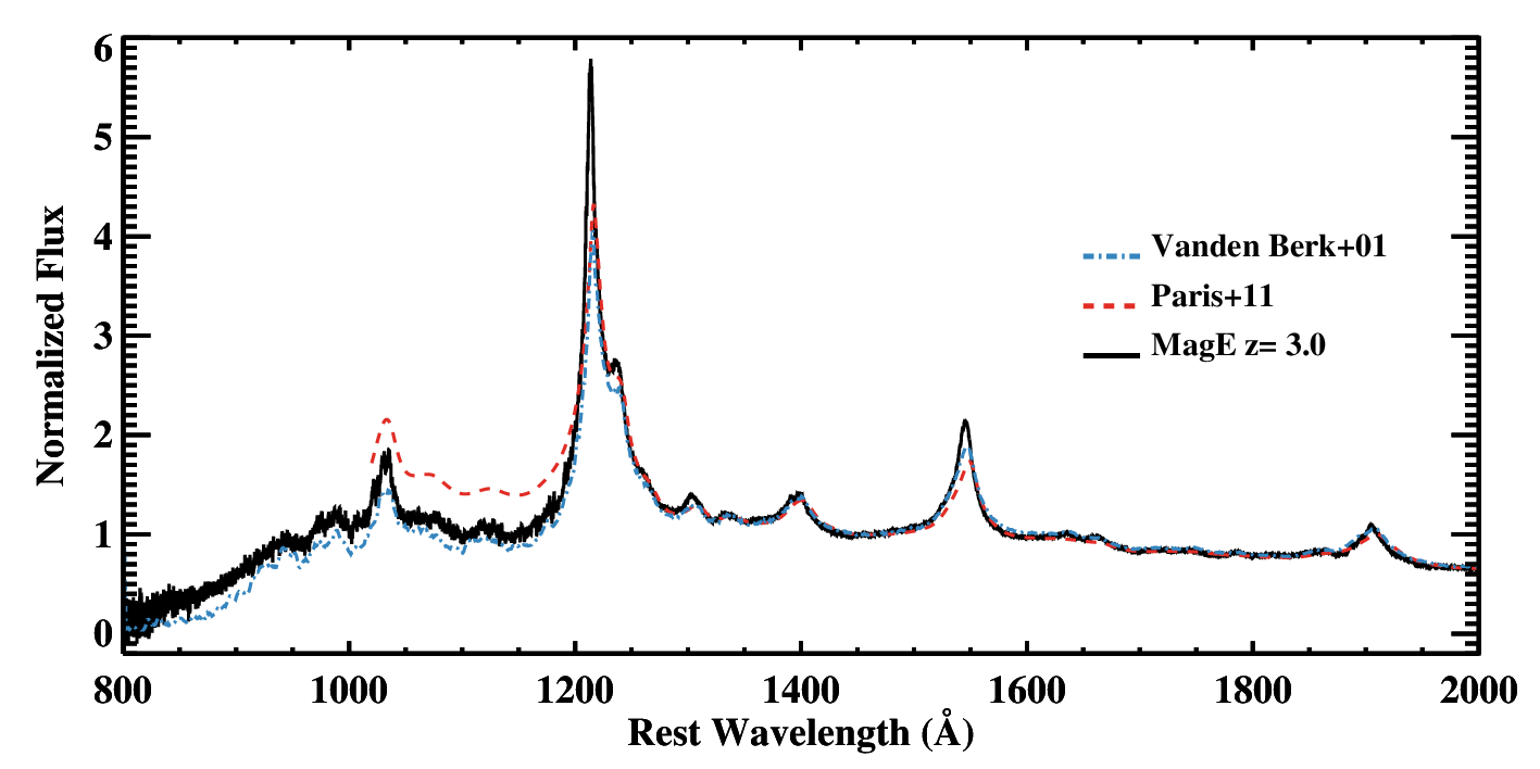
Leveraging the high and moderate resolution of these spectra, we construct a quasar template in a narrow redshift range () centered around . Despite our small sample size, the UV sensitivity of the MagE spectrograph allows us to extend available composite spectra at similar redshifts [39, e.g.] down to Å in the quasar rest frame, without resorting to the inclusion of higher redshift objects as, for instance, in the Vanden Berk et al. [69] template.
The final stack is produced by averaging the flux in the quasar spectra in their rest frame, after normalizing each spectrum by the continuum value as measured in a 10 Å window centered at 1400 Å. The resulting composite spectrum is shown in Figure 2, together with the template by Pâris et al. [39] and Vanden Berk et al. [69]. Excellent agreement is found in the continuum reward to Lyman, although each of the three templates exhibits different emission line properties. This discrepancy is expected due to variations in the quasar and host galaxy properties (e.g. metallicity, luminosity, redshift) in the three samples, especially given that the MagE composite is subject to a larger sample variance than the templates by Pâris et al. [39] and Vanden Berk et al. [69]. For Å, instead, there are noticeable differences related to how the absorption from the intergalactic medium (IGM) has been treated. Pâris et al. [39] correct their composite spectrum for the blanketing due to intervening Lyman forest clouds. Incidentally, we note that the ratio of the fluxes in the Pâris et al. [39] template and in the MagE spectrum between Å is fully consistent with the expected IGM absorption as recently measured by Becker et al. [4]. Conversely, the flux level in the composite spectrum by Vanden Berk et al. [69] is lower compared to our template. We ascribe this difference to the inclusion of quasars combined with the rapid redshift evolution of the IGM transmission that changes by between and [4].
IV. The mean free path of ionizing radiation
Because of the intervening IGM, the quasar composite spectrum at Å differs from a simple power-law extrapolation of the flux redward to the Lyman emission line (Figure 2). In particular, the nearly exponential flux decrement seen at Å contains information on the effective Lyman limit optical depth () which is related to the mean free path of ionizing photons (). By modeling the observed composite spectrum, it is therefore possible to extract information on the opacity that Lyman continuum photons experience, without the need of specifying the explicit form of the column density distribution function of the intervening absorbers.
In this section, we start by reviewing the adopted formalism that was first introduced by Prochaska et al. [45] and refined by O’Meara et al. [37], highlighting the elements that are most relevant to the present analysis. Next, we apply this methodology to the MagE composite spectrum and derive at .
IV.1. Formalism
We start by decomposing the observed quasar flux into three components,
| (1) |
where the power law accounts for a large-scale continuum, describes additional small-scale variations in the quasar spectral energy distribution, and models the wavelength-dependent effective optical depth arising from intervening absorbers. This last term includes the contribution of absorption both in the hydrogen Lyman series () and, at Å, in the Lyman continuum ()
| (2) |
In this equation, we further assume that the intrinsic quasar spectral energy distribution does not evolve as a function of wavelength over the narrow range of interest to our study ( Å). Throughout this analysis, we further neglect additional opacity due to the presence of metal lines, which produces only a very modest variation in the flux [4, ;], well within the uncertainties of our measurement. To model the power-law continuum, we fit individual spectra in regions free from emission lines, between Å, Å, and Å. The distribution of spectral indexes () agrees very well with the observed distribution in large samples of quasars [39, e.g.] with a median .
Next, to avoid the use of an explicit form for across the entire wavelength range, we model the continuum normalized spectrum () relative to the observed value at the Lyman limit Å
| (3) |
In this equation, we only need to provide the redshift evolution for , which in previous studies [37, e.g.] has been described by a power law of index
| (4) |
Here, is the redshift at which a photon of wavelength that is emitted at will be absorbed at the Lyman limit
| (5) |
In principle, one could fit for the free parameters in Equation (4), but, in practice, we find that data between Å do not constrain and independently. To account for this minor () but systematic effect, we evaluate numerically as
| (6) | |||
where is the line optical depth for the th transition in the Lyman series, and is the column density distribution function from O’Meara et al. [37] extrapolated to . The validity of this extrapolation is supported by results presented in Section V.
Once we have corrected the observed flux for the contribution of the Lyman series (), we only need to model the optical depth at the Lyman limit
| (7) |
which is related to the opacity seen at each redshift by ionizing photons that have been emitted at a frequency , integrated over the proper path-length from redshift to
| (8) |
In this equation, the integrand can be rewritten as the product of the redshift-dependent opacity and the photo-ionization cross section which, in redshift space, becomes
| (9) |
For the adopted cosmology,
| (10) |
where can be neglected between with an error of . As previously done in the literature [37], we can express the evolution of with the following functional form
| (11) |
but, again, we find that in practice data do not constrain . However, because is only weakly dependent on redshift [37, at ; ], we set for the reminder of this analysis.
In the end, the final model for the normalized flux corrected for absorption in the Lyman series becomes
| (12) |
with a free parameter. Finally, we define the mean free path as the distance between and at which .
IV.2. Results
We apply the formalism described in the previous subsection to the MagE composite spectra of both the color and non-color selected quasar samples. To find the best that describes the observed flux we adopt a minimum analysis in the wavelength range Å. The upper bound of this interval is chosen to avoid the quasar proximity region at Å, while the lower bound is set to avoid noisy data ( per pixel). Although we are selecting an optimal wavelength region, we have verified that the best fit value for is largely insensitive to our exact choice of the spectral range included in the analysis.


Errors on are derived via bootstrapping by modeling 1000 composite spectra from the color and non-color selected samples which we construct as described in Section III, but allowing for repetitions. Each composite spectrum is then normalized to the observed value at Å, after introducing a random variation up to in the normalization constant to account for additional uncertainties in the flux calibration. The two distributions of the best fit values for are shown in Figure 3.


There is a significant difference in the distributions of measured in color and non-color selected quasars. A Kolmogorov-Smirnov (KS) test for the color and non-color selected samples returns a KS statistic , and the associated probability that the two distributions in Figure 3 are drawn from the same parent population is . This systematic discrepancy is not only evident from the two distributions of , but it is also noticeable when inspecting the observed flux at Å in the composite spectra (Figure 4).
The different mean free path originates from the SDSS color selection algorithm that systematically misses blue quasars, a bias that has been previously discussed in Prochaska et al. [45] and Worseck & Prochaska [73]. Worseck & Prochaska [73] used mock quasar photometry to show that the SDSS color selection avoids quasars with between . They also concluded that, because the presence of a LLS along the line of sight “reddens” the quasar photometry shifting its color far from the stellar locus, SDSS preferentially selects quasars with intervening absorbers. Our study of the mean free path in samples of color and non-color selected quasars, together with the survey of LLSs in the next section, confirms the presence of this bias. For this reason, in the reminder of this paper we focus our statistical analysis on the non-color selected samples, providing results from the color selected sample for comparison only.
Figure 3 also reveals that both distributions of exhibit a tail towards high values of . We interpret this feature, visible in other studies [37, e.g.], as a consequence of sample variance in a set of quasars with a discrete number of intervening LLSs. As previously done in the literature, we express our best determination of the mean free path in the Universe using the median value of these distributions, together with the standard deviation computed after excluding significant outliers in the tail. The mean free path from both the color and non-color selected samples are and . The 5th, 25th, 75th, and 95th percentiles of the distribution of for the non-color selected sample are 68, 84, 126, and 184 respectively (in units of ).
Our new determination is higher but statistically consistent with the mean free path estimate of Faucher-Giguère et al. [19] at comparable redshift. These authors use an independent technique based on an analytic calculation for a given column density distribution function and find at . In Figure 5, our new mean free path estimates are also compared to the results of other studies that are based on a similar stacking analysis [45, 37, 74]. This figure shows that the mean free path of ionizing photons in the Universe smoothly evolves between . This redshift evolution is well described analytically by
| (13) |
with the frequency-dependent photoionization cross section and the 5-parameter column density distribution function by O’Meara et al. [37]. Here, has a redshift invariant shape, but the normalization evolves as a power law of index , with slightly favored by the data (see grey dashed line in Figure 5). According to this analytic form, that we normalize to match the observed at , photons can freely escape from the emitting sources by , the redshift at which the mean free path of ionizing photons equals the horizon .
Before concluding our discussion on the mean free path, we note that recent work by Rudie et al. [52] suggests a significantly shorter at compared to the estimate of O’Meara et al. [37]. This result would imply a shallower redshift evolution than what is presented in Figure 5. The analysis of Rudie et al. [52] relies on the measurement of the column density distribution function at , for which discrepant values exist in the literature. Due to the difficulties of measuring individual absorption line systems at column density above where saturation effects in the strongest lines of the Lyman series arise, we currently prefer the more direct measurements of the mean free path from the stacking analysis.
V. A survey of Lyman Limit systems
V.1. Catalogue of intervening LLSs
We compile a catalogue of intervening LLSs in two steps. First, we perform an automated search for flux discontinuities that can be attributed to absorption at the Lyman limit in the blue portion of the MagE spectra. This is done by comparing the observed flux in bins of 18Å to a model for the quasar continuum that is constructed by extrapolating the power law continuum measured at Å and including absorption from the Lyman- forest. Starting from the Lyman limit at the quasar redshift and moving blueward, the automatic procedure searches for flux discontinuities that can be modeled with an intervening LLS with in steps of redshift . Once a flux break is detected, the procedure compares models for the Lyman limit absorption at different column densities (in steps of ) to identify LLSs. Redshifts and column densities for these systems are stored.
To obtain a clean and complete census of LLSs at , we then inspect each quasar spectrum in search of a sharp flux decrement associated to the Lyman limit in the rest frame of LLSs (e.g. Figure 6.2), starting from the list of systems flagged by the automated search. Three of the authors (MF, JO, XP) have independently modeled the observed quasar flux by superimposing to an underlying continuum level both the Lyman series and the Lyman limits associated to intervening absorption systems. During this procedure, two different methods for establishing the quasar continuum have been adopted. The first method, previously used by O’Meara et al. [37], relies on the Telfer et al. [67] composite spectrum, which we adapt to the observed flux by allowing for a scale in normalization and a power law tilt. The second method, instead, assumes an extrapolation of the power law continuum measured at Å, to which we apply a correction for the Lyman- forest absorption as described in Section III. Both methods are found to yield consistent results. We emphasize that during this search, systems are selected purely based on their Lyman limit and Lyman series. Redshifts are determined by means of high order lines in the Lyman series to avoid a possible bias associated to the presence or lack of metal lines. Further, particular attention is given to the transmitted flux blueward of the Lyman limit which is needed to separate LLSs at from those at .


For the majority of cases (), at least two authors have agreed on the presence and redshift of a LLS. For the remaining cases in which discrepant models have been produced, three authors have jointly discussed the best model to describe the data. Not surprisingly, these discrepancies arise mostly at low and blueward of Å. We estimate that typical uncertainties of the hydrogen column density at range between dex, and depend on the spectrum . However, the quality of the data at Å quickly worsen, and a much larger uncertainty is associated to systems at . Because of our limited ability in identifying LLSs at these redshifts, in the following analysis we restrict our statistical survey to .
We further assess the completeness and purity of our catalogue of LLSs at using mock spectra. One of the authors (GW) generated four independent realizations of MagE spectra for each of the 105 quasars, assuming the same continuum and noise properties of the individual observed spectra and following the procedures detailed in Dall’Aglio et al. [13], Prochaska et al. [44], and Worseck & Prochaska [73]. These 420 mock spectra were subsequently analyzed independently by the other three authors (MF, JO, XP), following the same procedures adopted for the real data as described above. Results were then compared to the input catalogue of LLSs. From this comparison, we conclude that in of the cases (398/420 spectra), we are able to either correctly identify the presence of a LLS or to establish that no optically-thick system is present along the line of sight. Further, we successfully identify 189 of the 202 LLSs that are embedded in the mock spectra, corresponding to a completeness of . Thanks to the presence of the Lyman series, we are able to characterize the redshift of of the identified LLSs to within . Finally, 198 of the 207 systems that we flag as LLSs have in fact a column density , corresponding to a purity of . The remaining 9 systems are false positive that have column densities , corroborating our estimate for the error on the column density of dex.
V.2. Incidence of LLSs
Having a complete list of LLSs in our sample (Table 2), we can extract a statistical sample to quantify the number of LLSs per unit redshift by imposing additional selection criteria that define the total redshift path probed by our MagE survey (Figure 7). First, LLSs with a velocity from the quasar redshift are excluded because of their likely physical proximity to the quasar host galaxies. Further, when a LLS is detected at , the sharp flux decrement prevent us from searching additional systems at . Therefore, in each sightline, we consider the redshift range . If a LLS is detected, , and if , . Finally, because of the limited path of our survey beyond , we impose a limit . Individual values for and are summarized in Table 2, where we also highlight quasars that are in common with the previous surveys by Sargent et al. [54] and Lanzetta [32]. Considering the small overlap (10/105 sightlines), this survey is largely independent from previous efforts at comparable redshifts.
Given the total redshift path of the survey, we define the incidence of LLSs as the total number of systems detected within the useful redshift range divided by the integral of
| (14) |
In our statistical sample between , we find for the non-color selected sample and for the color selected sample. Here, the uncertainties are related to counting errors only. As previously found for the mean free path (Figure 3), there is a systematic difference between the color and non-color selected samples, albeit the two values of are marginally consistent due to the large uncertainties.
For the assumed cosmological model, we can further use the identity to recast the observed number of LLSs per unit redshift into a more physically motivated quantity that is proportional to the comoving number density of LLSs times their physical cross section [3, e.g.]. In this transformation,
| (15) |
and given that at , we find and for the non-color and color selected samples, respectively. In Figure 8, the results from our survey (blue square and red cross) are compared to previous determinations of in samples of LLSs that have been selected within narrow intervals of redshift [44, 50, 37]. Here, we also show the predicted at (grey X) that we compute from an extrapolation of the O’Meara et al. [37] assuming . The almost perfect agreement, consistent with what we previously found in the mean free path evolution, validate our previous assumption in constructing a model for the Lyman forest (see Section IV).
Finally, we estimate the contribution of LLSs to the observed . By definition,
| (16) |
with the comoving number density of LLSs and their physical cross section. At , the typical separation between LLSs therefore becomes [50, e.g.]
| (17) |
Compared to , it follows that systems with account for only of the observed mean free path. Similarly, integrating Equation 13 between and , we find that LLSs contribute to of the total Lyman limit optical depth for the assumed O’Meara et al. [37] . All together, our analysis reveals properties for the mean free path and for the number of LLSs that are consistent with previous determinations at other redshifts, implying a smooth evolution of the optically thick gas distribution across Gyr of cosmic history.
VI. Physical properties of Lyman limit systems
In this section, we exploit the quality of our MagE spectra to investigate the physical properties of LLSs. Here, we focus our analysis on a composite spectrum of LLSs to qualitatively explore typical values of metallicity and ionization parameters in a representative ensamble of systems that are selected purely based on their hydrogen column density between . A detailed analysis of the physical conditions in individual LLSs is deferred to future work.
In the previous sections, we showed how the number of LLSs found in color selected samples exceeds the number of intervening systems along non-color selected quasars. As discussed, this bias is due to the fact that absorption at the Lyman limit reddens the colors of these quasars, that are preferentially selected for spectroscopic follow-up because they separate from the stellar locus. Additional reddening may come from dust [71, 27], but studies of damped Lyman- systems (DLAs), at even higher column densities of , suggest only modest differences in the reddening of optical and radio selected quasars with intervening DLAs [26]. Thus, given two LLSs along a color selected quasar and a non-color selected quasar, there is no current indication that they will have largely different physical properties (e.g. their metal content), except perhaps an higher column density for the systems along color selected quasars. For this reason, in the remainder of this work, we combine the two populations of LLSs detected along color and non-color selected samples.
VI.1. The composite LLS spectrum
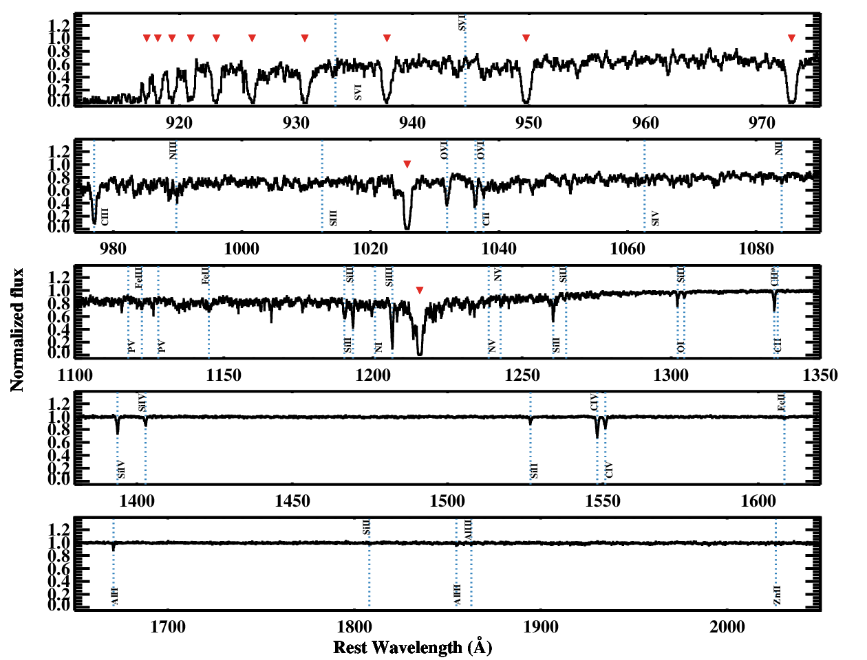
To generate a composite spectrum of LLSs, we first continuum normalize the quasar spectra by fitting a polynomial function to the data redward to the quasar Lyman emission lines, omitting regions where metal lines are detected in absorption. At wavelengths blueward to Lyman, instead, we generate a continuum model using a spline function that is constrained by the data in regions free from evident absorption arising in intervening systems. Between the quasar Lyman and Lyman emission lines, we further adopt a first guess for the continuum level using principle component analysis, following the procedure described in Pâris et al. [39]. Next, we median combine the normalized spectra in the rest-frame of the 38 LLSs that are part of our statistical sample at . In this case, a median is preferred over the arithmetic mean to attempt to preserve the definition of optical depth associated to each absorption line. As previously done for the quasar composite spectrum, the error array is derived via bootstrapping.
The LLS composite spectrum is shown in Figure 9, where we mark the position of metal transitions that are common in intervening systems. Besides the prominent hydrogen Lyman series, multiple transitions in different ionization states are detected, including O VI, Si IV and C IV, strong C III and Si III, singly ionized Si, C, Al, and O I. Similar absorption lines have been reported in a composite spectrum of LLSs at [44]. Although systems with are formally classified as LLSs, several studies have already investigated the typical metallicity and ionization state of DLAs with and of sub-DLAs or super-LLSs (SLLSs) with [16, 48, e.g.]. Conversely, with the exception of the pioneering study of Steidel [62], the metal properties and ionization states of LLSs with have been investigated in only a handful of systems [22, see appendix of] and a detailed study of a homogeneous and unbiased sample of LLSs is at present lacking.
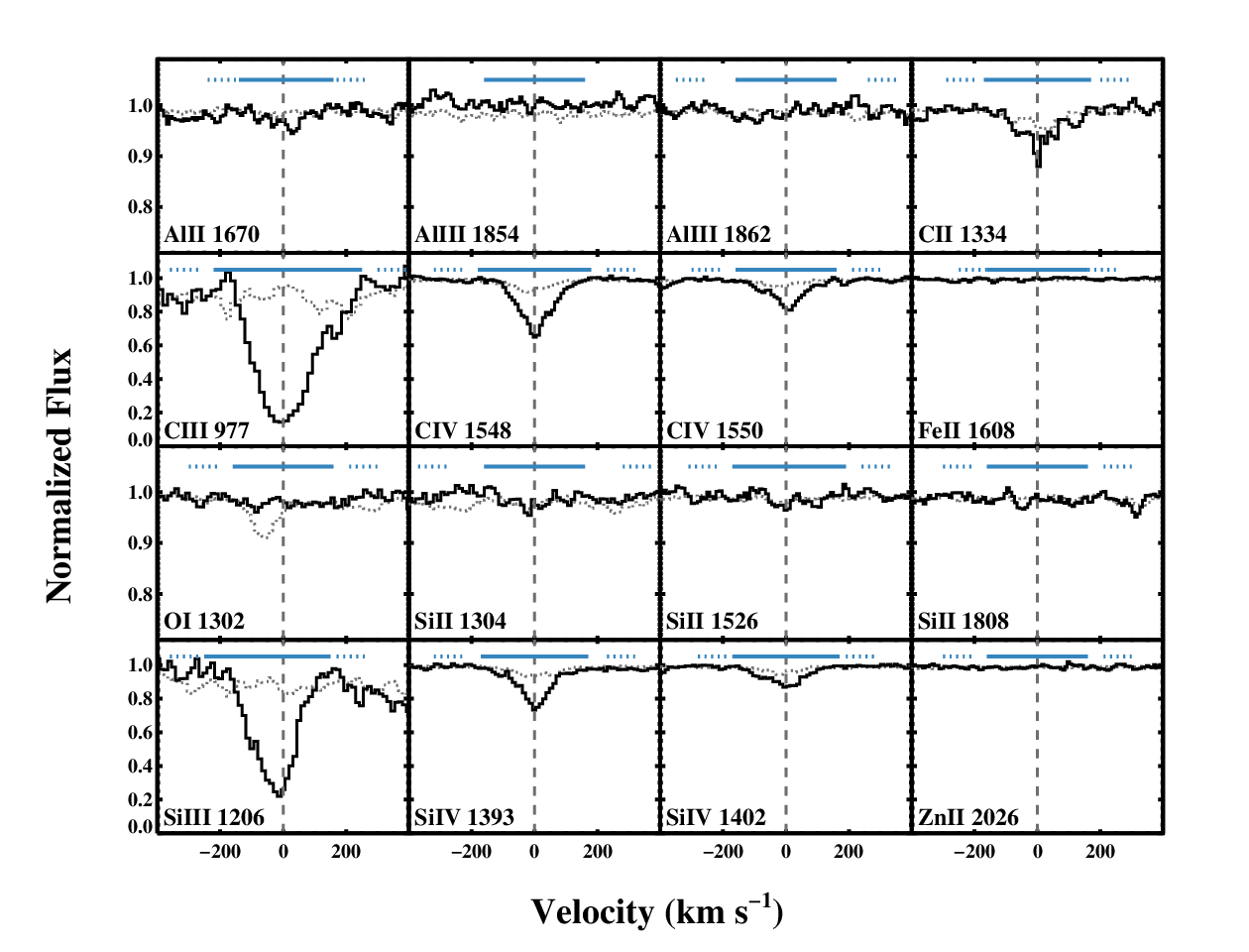
To explore the metal absorption properties of this sub-class of LLSs, we generate a second composite spectrum for the 20 LLSs in our statistical samples that exhibit an H I column density , as inferred from the absence of damping wings in the Lyman- line profile. In Figure 10, we show the line profiles of common metal transitions in this second composite spectrum at Å. Other transitions are detected at even shorter wavelength, but because of the limited sample size and the increasingly high contamination from the Lyman- forest blueward to Å, blends significantly affect our ability to reliably measure equivalent widths. However, given the predominance of doubly ionized transitions in LLSs [51, see Figure 9 or, e.g. ] and the fact that C III Å and Si III Å are clearly detected in the stack, we also include these transitions in our analysis. The most evident feature of Figure 10 is that, compared to the stack of all LLSs, the singly ionized species and O I are mostly undetected. A similar dichotomy between lower and higher ionization lines at different densities has been reported by Pieri et al. [40] in a composite spectrum of strong Lyman- forest absorbers, with .
To characterize the strength of the selected metal lines in the composite spectrum, we measure the line equivalent widths within a velocity window that is large enough to encompass the entire line profile. For the undetected lines, we fix instead the velocity window at , comparable to the width of the detected lines. A summary of these measurements is provided in Table 3, where we list limits for non detections.
Given the suggested connection between LLSs and the halo gas in the surroundings of galaxies (see Section VII), we compare the typical equivalent widths observed in LLSs and in the circumgalactic medium (CGM) of galaxies at similar redshifts. Using a composite of galaxy spectra at low resolution, Steidel et al. [63] have derived the typical equivalent widths of C II, Si IV, and C IV in the CGM of galaxies. The equivalent widths for LLSs are comparable to the values reported for the CGM only at the largest impact parameters, beyond kpc from the galaxy centers. At face value, this result implies that the majority of LLSs with do not arise from the innermost CGM of Lyman break galaxies (LBGs) with . However, this seems in contradiction to the empirical result that the halos of LBGs contain enough neutral gas to account for a significant fraction of the population of LLSs within 100 kpc from the galaxy centers [63]. This tension reveals a still incomplete understanding on the gas distribution around LBGs in connection to the population of LLSs, a gap that future studies need to address.

VI.2. Photo-ionization modeling
In this section, we use photo-ionization modeling to qualitatively investigate the typical metallicity and ionization conditions that are required to reproduce the equivalent widths seen in the composite spectrum of LLSs with at .
As evident from Figure 10, the majority of the metal transitions in this composite spectrum lie on the linear portion of the curve of growth, with the exception of C III and Si III that are most likely saturated at the spectral resolution of MagE. We can therefore directly map the observed equivalent widths into column densities, as listed in Table 3. Consistent values of column densities are also found via the apparent optical depth method [55]. Before proceeding, we emphasize that several effects confound the physical interpretation of column densities measured in composite spectra, including contamination from unrelated absorption lines or offsets in velocity between metal transitions and the systemic redshifts measured from hydrogen lines. Moreover, differential dust depletion and variation in the radiation field to which individual systems are exposed [12, see e.g.] complicate the interpretation of the measured column densities. Therefore, the listed column densities will be used only as proxy for the equivalent widths to gain qualitative insight on the physical properties of LLSs. A detailed analysis of individual systems will be presented in future work.
Results from the photo-ionization modeling are summarized in Figure 11, where we show the column densities of metal transitions as a function of and , normalized to the observed column densities or the corresponding limits listed in Table 3. Models are computed using the cloudy (v10.00) photo-ionization code [20], including both collisional ionization and photo-ionization at equilibrium and the Haardt & Madau [25] extragalactic UV background at . During our analysis, relative abundances of different elements are fixed to the solar values [2]. We also assume a typical hydrogen column density of , a value that is consistent with the median column density derived in random realizations of 20 LLSs that are drawn from the O’Meara et al. [37] at between . Further, the flux transmitted blueward to the Lyman limit is also consistent with a median .
Figure 11 reveals how the doubly and triply ionized C and Si transitions provide the most stringent constraints for the parameter, but they are mostly insensitive to the metallicity of the gas. Conversely, C II and Al II are the most constraining transitions for the metallicity, although degenerate with respect to . Combining all the independent constraints, we conclude that the equivalent widths observed in the composite spectrum of LLSs can be reproduced by gas that is significantly ionized (), and likely metal poor () [62, 47, cf.]. We should again emphasize that the use of the median composite spectrum to describe the entire population of LLSs is rather simplistic, as it does not capture information on the shape of the distribution. This is especially relevant given the recent claim by Lehner et al. [33] of a bimodal distribution of the metallicity in LLSs at , with one population peaking around and a second population centered at .
Our qualitative analysis suggests that LLSs are probably more enriched than the IGM at [60, e.g.], and possibly enriched to , the median metallicity observed in DLAs [48, e.g.]. Assuming a general picture of an increasingly higher metallicity in regions that are progressively closer to the site of star formation, where metals are produced, the enhanced metallicity of LLSs places this population of absorbers in proximity to or within galaxies halos that have been at least in part enriched by metals ejected from galaxies [58, e.g.].
VII. Lyman Limit systems and galaxy halos

In this last section, we expand the discussion of the connection between galaxies and LLSs, to which we alluded in the previous sections. Already from the first quasar surveys, it became evident how LLSs differ from the Lyman- forest [68, 54, 62] and that these absorbers are likely connected to galaxies. This idea has been subsequently reinforced by modern studies of the CGM [63, 10, 43, 53, 72, 11, 42, 65, e.g.] that show how cold, enriched, and partially ionized gas from which LLSs can originate fills galaxy halos both in the local and distant Universe. At the same time, several theoretical studies have addressed the connection between LLSs and galaxies in the high redshift Universe [28, 24, 30, 18, 21, 1, 70, 23, 49, e.g.]. Consistent findings are that LLSs arise from galaxy halos, in a mixture of infalling, static, and outflowing gas.
Having a complete view of the redshift distribution of LLSs across nearly Gyr of cosmic history (Figure 8), we explore with simple toy models how the evolution of relates to the evolution of the gas within galaxy halos. Similar investigations have been carried out in the literature by several authors. Recently, Ribaudo et al. [50] adopted an empirical approach to describe the evolution of LLSs in terms of the galaxy luminosity function and size-luminosity relation. These authors concluded that to account for the observed redshift dependence of , galaxies with have to contribute to the population of LLSs and that the physical cross section of the absorbing material rapidly evolves from to , remaining relatively constant afterwards. While instructive and empirical, this calculation does not provide a direct link between the halos in which galaxies resides and the incidence of LLSs. In this work, we revise this open question and propose possible scenarios for the co-evolution of LLSs and galaxy halos that is empirically traced by the redshift evolution of .
We construct a simple toy model of the Universe which we populate with dark matter halos with comoving number density . In our calculation, we assume a Sheth-Tormen halo mass function [59] computed as described in Dekel & Birnboim [14] and corrected to match the results of the Bolshoi simulation [29]. We then assign to each halo a characteristic virial radius , using redshift dependent scaling relations derived from the rockstar halo catalogues [5, 6] extracted from the Bolshoi simulation. Following the definition of in Equation (16), we compute the galaxy contribution to the observed as
| (18) |
with and the upper and lower mass limits and the covering factor of LLSs within twice the virial radius. Despite this formal definition, for a given cosmology, is only constraining , and it should be noted that we cannot discriminate between, e.g., a 10% covering factor within twice the virial radius and a 40% covering factor within one virial radius.
In this model, while and are fixed by the adopted cosmology, , , and are free parameters that may vary as a function of redshift and halo mass. The intrinsically one-dimensional nature of absorption line surveys is currently unable to disentangle the relative contribution of these parameters and, for this reason, we restrict to a minimal set of variables. First, we fix the upper limit to mimic the formation of a hot halo above a critical halo mass at which virial shocks become stable [14, e.g.]. This limit is higher than the typical value quoted for this critical halo mass (between ) to account for recent observational results which show a substantial amount of cold gas at or even beyond the mass scale at which hot halos are postulated to develop [42, 11]. However, because of the low number density of high mass halos, our result is largely insensitive to the assumed upper mass limit above . The second simplifying assumption is that, lacking strong priors for the functional form of , we assume a constant covering factor both in redshift and within the mass range specified by and . Thus, in our toy model, merely sets the absolute normalization of the predicted . Validation of this assumption awaits future theoretical and observational work.
The first model we construct, which we dub “minimal”, assumes that all the halos in the mass range contribute to the observed proportionally to their virial area (). As shown in Figure 12, a choice of at twice the virial radius ensures that this minimal model (red dotted line) matches the observed incidence of LLSs around . This covering factor lies in between theoretical predictions at comparable redshifts [21, 18, 58, 23] and what is inferred around LBGs [53] and quasar host galaxies [42].
The most evident problem with the minimal model is a complete inconsistency in the redshift evolution of . This failure cannot be resolved with simple scaling of and originates from an increase of almost a factor of in the virial area at fixed halo mass between , combined with an increase of a factor of in the number density of halos across a comparable redshift range. In principle, this tension could be resolved by assuming that LLSs do not co-evolve with the properties of halo gas. However, given the discussion presented in the previous sections, we believe that this explanation is unlikely, and attribute instead the mismatch between observations and the minimal model to having assumed that LLSs trace the CGM of a galaxy population with fixed halo mass at all redshifts. In the following, we present two possible ways to resolve the failure of the minimal model, which require either a rapid evolution in the typical mass interval from which LLSs arise, or that the size of the optically thick region around galaxies is decoupled from the size of the virial region.
In the second model, we attempt to overcome the shortcomings of the minimal model by introducing a redshift dependent lower mass limit. If we postulate that the majority of LLSs are associated to gas that is deposited in the halo by a feedback mechanism, we can naturally introduce a lower limit by assuming that halos with circular velocities below [15] are not able to retain a significant fraction of the ejected gas. For this reason, we define this second toy model as “wind” model. This additional constraint naturally leads to a mild evolution in the number density of halos that host LLSs between , accounting for the factor of excess encountered in the minimal model. More specifically, the lower mass limit evolves from at to at . Due to the increasing amplitude of the halo mass function as a function of time, the integrated number density of halos that contribute to LLSs slightly increases at first with redshift. By , instead, due to the progressively higher value of , the number density slightly declines with time.
However, the rapid increase in the virial area as a function of redshift would still cause this model to significantly overproduce LLSs at low redshifts, violating the observed . A better match to the observations is found if, instead, we fix the size of the CGM to the virial area at . Thanks to this ansatz, and by imposing a covering factor of , the wind model can account for the observed evolution between (blue dashed line in Figure 12). Having imposed a constant cross section for the CGM over the last Gyr of cosmic evolution, this model has only limited predictive power. Nevertheless, it is interesting to note that similar conclusions of an invariant size of the CGM have been reached independently by other studies of absorption line systems [9, 42, e.g.].
Given the multiple parameters that define in Equation 18, other models that reproduce the observed incidence of LLSs can be constructed with a different set of assumptions. For instance, a model in which rapidly increases with decreasing redshifts would naturally compensate the growth of the virial area by imposing that LLSs arise from progressively more massive and rarer halos at later times. Conveniently, cosmology offers a way to impose a rapid redshift evolution for . If we postulate that, as suggested by simulations [21, 70], a significant fraction of LLSs arise from dense streams of infalling gas that penetrate inside halos, we can construct a third “accretion” model where is set by a characteristic halo mass above which halos are significant fluctuations in the density field. Below this critical mass, halos reside within individual filaments of the cosmic web, where densities are comparable to the virial densities [14]. Therefore, below this mass threshold, we postulate that the typical gas densities are below what is required to form LLSs.
By imposing the condition , the accretion model (green dash dotted line in Figure 12) accounts for the observed redshift evolution of LLSs, without requiring any adjustment in the spatial extent of the CGM. In this model, however, the inclusion of low mass halos (down to ) forces us to adopt a lower covering factor than what was assumed in previous models ( within virial radius). While the actual value of is likely higher at most redshifts, this model provides a qualitative illustration on how the rapid redshift evolution of relegates LLSs to the CGM of progressively rarer halos, thus compensating for the large increase in the virial area at fixed halo mass with cosmic time.
Finally, Figure 12 further illustrates that none of the proposed toy models is able to reproduce the steep rise in beyond . Clearly, a sudden increase in the extent of the CGM for would reproduce the observed trend [50]. However, it is unclear why should represent a special epoch in the evolution of the CGM. Instead, we argue that the different redshift evolution that is observed for is associated to an increasingly higher contribution of the IGM to the population of LLSs. This is because at progressively higher redshifts the overdensities at which LLSs form approach and exceed the halo virial density and, furthermore, the extragalactic UV background decreases.
A simple calculation can be used to illustrate this argument. For clouds illuminated by UV background radiation, hydrogen densities around are required for the gas to retain of neutral hydrogen [21, e.g. Appendix B of]. This threshold is comparable to the virial densities of halos at , while by redshift , typical virial densities equal , the value at which the neutral fraction approaches for a constant UV background. A similar picture is also supported by detailed radiative transfer calculations in numerical simulations that are able to reproduce the abundance of LLSs between [36].
VIII. Summary and Conclusions
In this paper, we have presented results of a survey of 105 quasars at conducted with the blue sensitive MagE spectrograph at the Magellan Clay telescope. The high signal-to-noise and moderate resolution data have been analyzed to investigate the properties of optically-thick hydrogen at , a redshift interval that has been not studied in a systematic way by previous surveys. Our principal findings can be summarized as it follows.
- –
By modeling the composite spectrum of quasars that are selected independently of their optical colors, we have estimated the mean free path of ionizing photons to be in the Universe. This value, together with previous determinations at different redshifts from the literature, favors a redshift evolution of in the amplitude of the column density distribution function in the form , and implies that the Universe becomes transparent to ionizing radiation around redshift . During this analysis, we have also confirmed the presence of a previously discovered selection bias in SDSS that systematically misses blue quasars in proximity to the stellar locus.
- –
We have conducted a survey of LLSs in the wavelength range Å and we have characterized the number of LLSs per unit redshift at . For the adopted cosmological model, this quantity translates into . Our new determination is fully consistent with previous measurements at lower and higher redshifts, implying a smooth evolution of between and . Combined with our measurement of the mean free path at the same redshift, we have concluded that LLSs with contribute to of total mean free path at .
- –
With the aid of photo-ionization modeling, we have inferred that a population of ionized () and likely metal poor () LLSs is required to reproduced the metal line equivalent widths observed in a composite spectrum of 20 LLSs with at .
- –
We have proposed three simple toy models to describe the redshift evolution of LLSs in connection to galaxies. Our main finding is that a model in which LLSs arise in halos of fixed mass at all redshifts drastically fails to reproduce the observed number of LLSs per unit redshift. Successful models require either a rapid redshift evolution of the minimum mass at which LLSs form or a redshift invariant spatial extent of the CGM in the last Gyr of cosmic evolution. In all cases, however, the rapid evolution observed in at is not accounted for, and we speculate that an increasingly higher contribution from gas within the IGM is required.
In conclusion, our MagE survey of quasars has provided the missing pieces in a consistent picture of the cosmological evolution of optically thick gas between . The redshift evolution of the mean free path of ionizing radiation and the incidence of LLSs are now well characterized with homogeneous techniques across Gyr of cosmic history, albeit with some controversy at . Our survey has also provided a homogeneous sample of hydrogen-selected LLSs that can be exploited to characterize the physical properties these absorbers and their connections to galaxies at . The analysis presented in this paper has offered only a first glimpse of the typical metallicity of LLSs, together with viable ways to model the observed evolution of . Clearly, our work does not provide the final answer to some of the riddles we encountered along the way, including the lower equivalent widths of metal lines in a composite of LLSs compared to what measured in a composite spectrum of galaxies. The task of formulating a coherent picture for the co-evolution of galaxies and LLSs is therefore a challenge that future studies will have to undertake.
References
- [1] Altay, G., Theuns, T., Schaye, J., Crighton, N. H. M., & Dalla Vecchia, C. 2011, ApJ, 737, L37
- [2] Asplund, M., Grevesse, N., Sauval, A. J., & Scott, P. 2009, ARA&A, 47, 481
- [3] Bahcall, J. N., & Peebles, P. J. E. 1969, ApJ, 156, L7
- [4] Becker, G. D., Hewett, P. C., Worseck, G., & Prochaska, J. X. 2013, MNRAS, 430, 2067
- [5] Behroozi, P. S., Wechsler, R. H., & Wu, H.-Y. 2013, ApJ, 762, 109
- [6] Behroozi, P. S., Wechsler, R. H., Wu, H.-Y., et al. 2013, ApJ, 763, 18
- [7] Bochanski, J. J., Hennawi, J. F., Simcoe, R. A., et al. 2009, PASP, 121, 1409
- [8] Bouché, N., Lehnert, M. D., Aguirre, A., Péroux, C., & Bergeron, J. 2007, MNRAS, 378, 525
- [9] Chen, H.-W. 2012, MNRAS, 427, 1238
- [10] Chen, H.-W., Wild, V., Tinker, J. L., et al. 2010, ApJ, 724, L176
- [11] Churchill, C. W., Nielsen, N. M., Kacprzak, G. G., & Trujillo-Gomez, S. 2013, ApJ, 763, L42
- [12] Cooke, R., Pettini, M., Jorgenson, R. A., et al. 2013, MNRAS, 431, 1625
- [13] Dall’Aglio, A., Wisotzki, L., & Worseck, G. 2008, A&A, 491, 465
- [14] Dekel, A., & Birnboim, Y. 2006, MNRAS, 368, 2
- [15] Dekel, A., & Silk, J. 1986, ApJ, 303, 39
- [16] Dessauges-Zavadsky, M., Péroux, C., Kim, T.-S., D’Odorico, S., & McMahon, R. G. 2003, MNRAS, 345, 447
- [17] Faucher-Giguère, C.-A., Lidz, A., Zaldarriaga, M., & Hernquist, L. 2009, ApJ, 703, 1416
- [18] Faucher-Giguère, C.-A., & Kereš, D. 2011, MNRAS, 412, L118
- [19] Faucher-Giguère, C.-A., Lidz, A., Hernquist, L., & Zaldarriaga, M. 2008, ApJ, 688, 85
- [20] Ferland, G. J., Korista, K. T., Verner, D. A., et al. 1998, PASP, 110, 761
- [21] Fumagalli, M., Prochaska, J. X., Kasen, D., et al. 2011a, MNRAS, 418, 1796
- [22] Fumagalli, M., O’Meara, J. M., & Prochaska, J. X. 2011b, Science, 334, 1245
- [23] Fumagalli, M., Hennawi, J. F., Prochaska, J. X., et al. 2013, arXiv:1308.1669
- [24] Gardner, J. P., Katz, N., Hernquist, L., & Weinberg, D. H. 2001, ApJ, 559, 131
- [25] Haardt, F., & Madau, P. 2012, ApJ, 746, 125
- [26] Jorgenson, R. A., Wolfe, A. M., Prochaska, J. X., et al. 2006, ApJ, 646, 730
- [27] Kaplan, K. F., Prochaska, J. X., Herbert-Fort, S., Ellison, S. L., & Dessauges-Zavadsky, M. 2010, PASP, 122, 619
- [28] Katz, N., Weinberg, D. H., Hernquist, L., & Miralda-Escude, J. 1996, ApJ, 457, L57
- [29] Klypin, A. A., Trujillo-Gomez, S., & Primack, J. 2011, ApJ, 740, 102
- [30] Kohler, K., & Gnedin, N. Y. 2007, ApJ, 655, 685
- [31] Komatsu, E., Smith, K. M., Dunkley, J., et al. 2011, ApJS, 192, 18
- [32] Lanzetta, K. M. 1991, ApJ, 375, 1
- [33] Lehner, N., Howk, J. C., Tripp, T. M., et al. 2013, ApJ, 770, 138
- [34] Madau, P., Haardt, F., & Rees, M. J. 1999, ApJ, 514, 648
- [35] Marshall, J. L., Burles, S., Thompson, I. B., et al. 2008, Proc. SPIE, 7014
- [36] McQuinn, M., Oh, S. P., & Faucher-Giguère, C.-A. 2011, ApJ, 743, 82
- [37] O’Meara, J. M., Prochaska, J. X., Worseck, G., Chen, H.-W., & Madau, P. 2013, ApJ, 765, 137
- [38] Pâris, I., Petitjean, P., Aubourg, É., et al. 2012, A&A, 548, A66
- [39] Pâris, I., Petitjean, P., Rollinde, E., et al. 2011, A&A, 530, A50
- [40] Pieri, M. M., Frank, S., Weinberg, D. H., Mathur, S., & York, D. G. 2010, ApJ, 724, L69
- [41] Prochaska, J. X. 1999, ApJ, 511, L71
- [42] Prochaska, J. X., Hennawi, J. F., & Simcoe, R. A. 2013, ApJ, 762, L19
- [43] Prochaska, J. X., Weiner, B., Chen, H.-W., Mulchaey, J., & Cooksey, K. 2011, ApJ, 740, 91
- [44] Prochaska, J. X., O’Meara, J. M., & Worseck, G. 2010, ApJ, 718, 392
- [45] Prochaska, J. X., Worseck, G., & O’Meara, J. M. 2009, ApJ, 705, L113
- [46] Prochaska, J. X., O’Meara, J. M., Herbert-Fort, S., et al. 2006, ApJ, 648, L97
- [47] Prochaska, J. X., & Burles, S. M. 1999, AJ, 117, 1957
- [48] Rafelski, M., Wolfe, A. M., Prochaska, J. X., Neeleman, M., & Mendez, A. J. 2012, ApJ, 755, 89
- [49] Rahmati, A., Pawlik, A. H., Raičevic, M., & Schaye, J. 2013, MNRAS, 430, 2427
- [50] Ribaudo, J., Lehner, N., & Howk, J. C. 2011, ApJ, 736, 42
- [51] Ribaudo, J., Lehner, N., Howk, J. C., et al. 2011, ApJ, 743, 207
- [52] Rudie, G. C., Steidel, C. C., Shapley, A. E., & Pettini, M. 2013, ApJ, 769, 146
- [53] Rudie, G. C., Steidel, C. C., Trainor, R. F., et al. 2012, ApJ, 750, 67
- [54] Sargent, W. L. W., Steidel, C. C., & Boksenberg, A. 1989, ApJS, 69, 703
- [55] Savage, B. D., & Sembach, K. R. 1991, ApJ, 379, 245
- [56] Schlegel, D. J., Finkbeiner, D. P., & Davis, M. 1998, ApJ, 500, 525
- [57] Schneider, D. P., Richards, G. T., Hall, P. B., et al. 2010, AJ, 139, 2360
- [58] Shen, S., Madau, P., Guedes, J., et al. 2013, ApJ, 765, 89
- [59] Sheth, R. K., & Tormen, G. 1999, MNRAS, 308, 119
- [60] Simcoe, R. A. 2011, ApJ, 738, 159
- [61] Songaila, A., & Cowie, L. L. 2010, ApJ, 721, 1448
- [62] Steidel, C. C. 1990, ApJS, 74, 37
- [63] Steidel, C. C., Erb, D. K., Shapley, A. E., et al. 2010, ApJ, 717, 289
- [64] Stengler-Larrea, E. A., Boksenberg, A., Steidel, C. C., et al. 1995, ApJ, 444, 64
- [65] Stocke, J. T., Keeney, B. A., Danforth, C. W., et al. 2013, ApJ, 763, 148
- [66] Storrie-Lombardi, L. J., McMahon, R. G., Irwin, M. J., & Hazard, C. 1994, ApJ, 427, L13
- [67] Telfer, R. C., Zheng, W., Kriss, G. A., & Davidsen, A. F. 2002, ApJ, 565, 773
- [68] Tytler, D. 1982, Nature, 298, 427
- [69] Vanden Berk, D. E., Richards, G. T., Bauer, A., et al. 2001, AJ, 122, 549
- [70] van de Voort, F., Schaye, J., Altay, G., & Theuns, T. 2012, MNRAS, 421, 2809
- [71] Vladilo, G., Centurión, M., Levshakov, S. A., et al. 2006, A&A, 454, 151
- [72] Werk, J. K., Prochaska, J. X., Thom, C., et al. 2013, ApJS, 204, 17
- [73] Worseck, G., & Prochaska, J. X. 2011, ApJ, 728, 23
- [74] Worseck et al. 2013, in preparation
| Name | R.A. | Dec. | aaStatistical error on the quasar redshift from broad emission lines. | bbCorresponding error on the quasar redshift in velocity. | NotesccC: color selected; NC: non color selected; B: broad absorption line quasar (visually classified) | Date | Exposure | Slit | S/N at 5500Å | |
|---|---|---|---|---|---|---|---|---|---|---|
| (J2000) | (J2000) | () | (yymmdd) | (sec) | (”) | |||||
| FBQSJ0002+0021 | 00:02:21.11 | +00:21:49.3 | 3.072 | 0.007 | 521 | NC | 120713 | 3000 | 0.7 | 9.7 |
| Q0038-4041 | 00:40:49.50 | -40:25:14.0 | 2.977 | 0.009 | 714 | NC | 120715 | 2700 | 0.7 | 26.0 |
| LBQS0041-2638 | 00:43:42.80 | -26:22:11.0 | 3.058 | 0.007 | 521 | NC | 091223 | 2000 | 0.7 | 16.0 |
| LBQS0047-3050 | 00:50:20.10 | -30:34:21.0 | 2.967 | 0.007 | 521 | NC | 091223 | 1000 | 0.7 | 13.3 |
| UM669 | 01:05:16.80 | -18:46:42.0 | 3.041 | 0.007 | 521 | NC | 091223 | 1000 | 0.7 | 20.1 |
| Q0130-403 | 01:33:01.90 | -40:06:28.0 | 3.031 | 0.007 | 521 | NC | 091222 | 1200 | 0.7 | 30.3 |
| UM148 | 01:56:36.00 | +04:45:28.0 | 3.001 | 0.007 | 521 | NC | 091223 | 1000 | 0.7 | 14.1 |
| CTS0418 | 02:17:41.80 | -37:01:00.0 | 2.916 | 0.007 | 521 | NC | 091222 | 900 | 0.7 | 26.2 |
| H0216+0803 | 02:18:57.30 | +08:17:28.0 | 3.001 | 0.010 | 714 | NC | 100814 | 1200 | 0.7 | 20.4 |
| CTS0220 | 02:41:22.70 | -36:33:19.0 | 3.109 | 0.007 | 521 | NC | 091223 | 900 | 0.7 | 16.2 |
| Q0244-302 | 02:46:34.20 | -30:04:55.0 | 3.088 | 0.007 | 521 | NC | 091222 | 1000 | 0.7 | 11.2 |
| CTS0424 | 03:16:43.80 | -56:51:45.0 | 3.036 | 0.007 | 521 | NC | 091222/23 | 2200 | 0.7 | 32.4 |
| CTS0238 | 03:30:10.30 | -46:26:15.0 | 3.112 | 0.007 | 521 | NC | 091222 | 1100 | 0.7 | 15.1 |
| Q0351-3740 | 03:53:08.50 | -37:40:54.0 | 2.952 | 0.007 | 521 | NC | 091222 | 1200 | 0.7 | 22.3 |
| Q0351-390 | 03:53:19.20 | -38:55:56.0 | 3.007 | 0.010 | 714 | NC | 091223 | 600 | 0.7 | 23.9 |
| CTS0246 | 04:04:01.90 | -33:35:00.0 | 3.042 | 0.007 | 521 | NC | 091223 | 800 | 0.7 | 20.4 |
| CTQ0247 | 04:07:18.00 | -44:10:14.0 | 3.021 | 0.010 | 714 | NC | 091223 | 1000 | 0.7 | 25.6 |
| CTS0648 | 04:39:06.90 | -50:47:40.0 | 2.947 | 0.007 | 521 | NC | 091222 | 1200 | 0.7 | 21.5 |
| CTS0260 | 04:45:52.00 | -31:58:43.0 | 2.722 | 0.006 | 521 | NC | 091222 | 900 | 0.7 | 22.0 |
| H0449-1325 | 04:51:42.60 | -13:20:33.0 | 3.107 | 0.007 | 521 | NC | 091222 | 1100 | 0.7 | 23.6 |
| CTS0269 | 05:17:42.20 | -37:54:46.0 | 3.045 | 0.007 | 521 | NC | 091222 | 800 | 0.7 | 21.7 |
| Q0642-506 | 06:43:27.00 | -50:41:13.0 | 3.107 | 0.007 | 521 | NC | 091222 | 900 | 0.7 | 19.9 |
| GB6J0833+1123 | 08:33:14.36 | +11:23:36.3 | 2.986 | 0.007 | 521 | NC | 091222/23,110329 | 3600 | 0.7 | 33.2 |
| SDSSJ0904+1309 | 09:04:23.37 | +13:09:20.7 | 2.975 | 0.007 | 521 | NC | 091222/23 | 1800 | 0.7 | 38.1 |
| HE0940-1050 | 09:42:53.40 | -11:04:25.0 | 3.076 | 0.007 | 521 | NC | 091222 | 800 | 0.7 | 36.5 |
| CTS0281 | 09:52:33.30 | -23:53:48.0 | 2.904 | 0.008 | 631 | NC | 091222,110329 | 2400 | 0.7 | 28.8 |
| PKS1010-427 | 10:12:37.80 | -42:58:37.8 | 2.962 | 0.007 | 521 | NC | 091223 | 1000 | 0.7 | 16.6 |
| TXS1033+137 | 10:36:26.88 | +13:26:51.7 | 3.098 | 0.007 | 521 | NC | 110328 | 1200 | 0.7 | 19.9 |
| CTS0296 | 10:58:09.20 | -26:05:39.0 | 2.887 | 0.007 | 521 | NC | 091222 | 900 | 0.7 | 29.8 |
| HS1200+1539 | 12:03:31.29 | +15:22:54.7 | 2.985 | 0.007 | 521 | NC | 110328,120711 | 2100 | 0.7 | 41.9 |
| LBQS1209+1524 | 12:12:32.04 | +15:07:25.6 | 3.067 | 0.007 | 521 | NC | 110329 | 2400 | 0.7 | 21.1 |
| Q1210-1049 | 12:12:52.10 | -11:06:10.0 | 2.938 | 0.007 | 521 | NC | 120712 | 2700 | 0.7 | 17.0 |
| LBQS1223+1753 | 12:26:07.19 | +17:36:49.8 | 2.953 | 0.009 | 654 | NC | 110329 | 1200 | 0.7 | 23.4 |
| SDSSJ1241+1230 | 12:41:58.18 | +12:30:59.3 | 2.979 | 0.009 | 714 | NC | 120711 | 3600 | 0.7 | 12.3 |
| CTS0320 | 13:17:44.10 | -31:47:14.0 | 2.965 | 0.007 | 521 | NC | 110328 | 2200 | 0.7 | 19.7 |
| LBQS1345-0120 | 13:48:16.65 | -01:35:09.9 | 2.957 | 0.007 | 521 | NC | 120713 | 2700 | 0.7 | 26.0 |
| CTS0331 | 14:01:38.00 | -13:46:10.0 | 3.022 | 0.011 | 792 | NC | 120715 | 2700 | 0.7 | 20.4 |
| Q1406+123 | 14:08:38.92 | +12:07:09.6 | 2.944 | 0.007 | 521 | NC | 120714 | 3000 | 0.7 | 33.2 |
| Q1455+123 | 14:58:07.50 | +12:09:37.8 | 3.057 | 0.007 | 521 | NC | 120712 | 3000 | 0.7 | 18.6 |
| Q1508+087 | 15:10:47.37 | +08:35:35.2 | 2.999 | 0.011 | 792 | NC | 120713 | 3300 | 0.7 | 13.1 |
| Q1510+105 | 15:13:04.41 | +10:23:30.8 | 3.064 | 0.007 | 521 | NC | 120715 | 3600 | 0.7 | 23.0 |
| SDSSJ1559+1631 | 15:59:36.89 | +16:31:01.5 | 3.072 | 0.009 | 631 | NC | 120715 | 3600 | 0.7 | 18.0 |
| SDSSJ1604+1645 | 16:04:41.47 | +16:45:38.3 | 2.888 | 0.010 | 792 | NC-B | 100813 | 2900 | 0.7 | 56.7 |
| Q1623+155 | 16:25:47.21 | +15:27:21.1 | 3.060 | 0.009 | 631 | NC | 120712 | 2700 | 0.7 | 14.3 |
| PMNJ1837-5848 | 18:37:53.80 | -58:48:09.0 | 3.041 | 0.007 | 521 | NC | 120712/15 | 5700 | 0.7 | 6.2 |
| Q2117-4600 | 21:21:11.50 | -45:47:58.0 | 2.957 | 0.007 | 521 | NC | 120715 | 3600 | 0.7 | 8.9 |
| Q2119-4307A | 21:22:28.70 | -42:54:38.0 | 2.952 | 0.007 | 521 | NC-B | 120713 | 3600 | 0.7 | 16.4 |
| Q2135-1335 | 21:27:45.40 | -13:22:13.0 | 2.928 | 0.007 | 521 | NC | 100813/14 | 2700 | 0.7 | 21.5 |
| FBQS2129+0037 | 21:29:16.60 | +00:37:56.6 | 2.961 | 0.007 | 521 | NC | 100814 | 1100 | 0.7 | 26.3 |
| CTS0358 | 21:41:44.40 | -38:40:41.0 | 3.102 | 0.009 | 631 | NC | 120715 | 3300 | 0.7 | 22.0 |
| PSGS2144+0542 | 21:47:22.26 | +05:56:19.5 | 2.909 | 0.007 | 521 | NC | 120715 | 3600 | 0.7 | 12.2 |
| SDSSJ2201+1256 | 22:01:16.75 | +12:56:36.4 | 2.927 | 0.009 | 714 | NC | 120713 | 3000 | 0.7 | 17.5 |
| FBQSJ2207+0101 | 22:07:08.32 | +01:01:25.2 | 2.904 | 0.007 | 521 | NC | 120715 | 3000 | 0.7 | 26.2 |
| PC2211+0119 | 22:14:27.80 | +01:34:57.0 | 3.109 | 0.007 | 521 | NC | 120713 | 3000 | 0.7 | 20.6 |
| LBQS2231-0015 | 22:34:08.99 | +00:00:01.6 | 3.025 | 0.010 | 714 | NC | 100813 | 1200 | 0.7 | 31.3 |
| HE2243-6031 | 22:47:09.10 | -60:15:45.0 | 3.005 | 0.011 | 792 | NC | 100813,120712 | 1500 | 0.7 | 56.1 |
| UM659 | 23:14:07.20 | -03:25:28.0 | 3.056 | 0.009 | 631 | NC | 120712 | 2700 | 0.7 | 14.6 |
| PKS2314-340 | 23:16:43.39 | -33:49:12.5 | 2.963 | 0.007 | 521 | NC-B | 100813 | 1200 | 0.7 | 24.2 |
| FBQS2330-0120 | 23:30:54.40 | -01:20:53.0 | 2.910 | 0.007 | 521 | NC | 100814 | 1500 | 0.7 | 14.0 |
| FBQSJ2339+0030 | 23:39:30.00 | +00:30:17.3 | 3.053 | 0.007 | 521 | NC | 120712 | 2700 | 0.7 | 20.1 |
| UM184 | 23:50:57.87 | -00:52:09.9 | 3.021 | 0.010 | 714 | NC | 120712 | 3000 | 0.7 | 23.8 |
| SDSSJ0010-0037 | 00:10:22.17 | -00:37:01.3 | 3.153 | 0.007 | 521 | C | 100814 | 1200 | 0.7 | 12.3 |
| SDSSJ0043-0015 | 00:43:23.43 | -00:15:52.6 | 2.829 | 0.008 | 631 | C | 100814 | 1200 | 0.7 | 18.6 |
| SDSSJ0125-1027 | 01:25:30.85 | -10:27:39.8 | 3.356 | 0.008 | 521 | C | 100813/14 | 2400 | 0.7 | 27.8 |
| SDSSJ0139-0824 | 01:39:01.40 | -08:24:43.9 | 3.016 | 0.010 | 714 | C | 091223,100813/14 | 3600 | 0.7 | 21.0 |
| SDSSJ0145-0945 | 01:45:16.59 | -09:45:17.3 | 2.732 | 0.006 | 521 | C | 100813 | 900 | 0.7 | 37.0 |
| SDSSJ0145-0945B | 01:45:16.76 | -09:45:17.9 | 2.731 | 0.006 | 521 | C | 100813 | 1500 | 0.7 | 14.9 |
| SDSSJ0148-0907 | 01:48:50.64 | -09:07:12.8 | 3.322 | 0.008 | 521 | C | 100814 | 1200 | 0.7 | 22.4 |
| SDSSJ0209-0005 | 02:09:50.70 | -00:05:06.4 | 2.858 | 0.007 | 521 | C | 100814 | 900 | 0.7 | 37.2 |
| SDSSJ0251-0737 | 02:51:51.20 | -07:37:07.7 | 3.084 | 0.007 | 521 | C | 091223 | 1000 | 0.7 | 12.9 |
| SDSSJ0303-0023 | 03:03:41.04 | -00:23:21.8 | 3.229 | 0.007 | 521 | C | 091223 | 900 | 0.7 | 24.4 |
| SDSSJ0304-0008 | 03:04:49.86 | -00:08:13.4 | 3.297 | 0.009 | 631 | C | 091223,100814 | 2000 | 0.7 | 34.0 |
| SDSSJ0338-0005 | 03:38:54.77 | -00:05:20.9 | 3.053 | 0.010 | 714 | C | 091223 | 1000 | 0.7 | 15.7 |
| SDSSJ0859+0205 | 08:59:59.15 | +02:05:19.7 | 2.979 | 0.009 | 654 | C | 091222/23 | 2400 | 0.7 | 27.9 |
| SDSSJ0908+0658 | 09:08:32.28 | +06:58:53.8 | 3.062 | 0.007 | 521 | C | 110329 | 1200 | 0.7 | 14.5 |
| SDSSJ0915+0549 | 09:15:46.68 | +05:49:42.7 | 2.976 | 0.007 | 521 | C | 110329 | 1200 | 0.7 | 23.7 |
| SDSSJ0931-0000 | 09:31:53.12 | -00:00:51.0 | 3.209 | 0.007 | 521 | C | 091223 | 1100 | 0.7 | 16.7 |
| SDSSJ0937+0417 | 09:37:15.38 | +04:17:37.6 | 3.127 | 0.007 | 521 | C | 091223 | 1100 | 0.7 | 16.6 |
| SDSSJ0942+0422 | 09:42:02.04 | +04:22:44.6 | 3.283 | 0.009 | 631 | C | 091222/23 | 1500 | 0.7 | 40.1 |
| SDSSJ0947+1421 | 09:47:34.20 | +14:21:17.0 | 3.041 | 0.007 | 521 | C | 110328 | 900 | 0.7 | 28.3 |
| SDSSJ1004+0018 | 10:04:28.43 | +00:18:25.6 | 3.050 | 0.009 | 631 | C | 091222/23 | 2100 | 0.7 | 24.9 |
| SDSSJ1015+1118 | 10:15:39.35 | +11:18:15.9 | 2.913 | 0.007 | 521 | C | 110329 | 1200 | 0.7 | 18.7 |
| SDSSJ1019+0825 | 10:19:54.53 | +08:25:15.0 | 2.989 | 0.007 | 521 | C | 110328 | 1200 | 0.7 | 23.7 |
| SDSSJ1025+0452 | 10:25:09.64 | +04:52:46.7 | 3.243 | 0.007 | 521 | C | 091223 | 900 | 0.7 | 20.2 |
| SDSSJ1205-0048 | 12:05:32.23 | -00:48:48.2 | 2.986 | 0.007 | 521 | C | 110328 | 1200 | 0.7 | 17.8 |
| SDSSJ1405+0507 | 14:05:21.67 | +05:07:44.4 | 2.994 | 0.007 | 521 | C-B | 110329 | 1200 | 0.7 | 18.0 |
| SDSSJ1432+1139 | 14:32:12.86 | +11:39:53.1 | 3.006 | 0.010 | 714 | C-B | 110329 | 1000 | 0.7 | 13.8 |
| SDSSJ1459+0024 | 14:59:07.18 | +00:24:01.2 | 3.024 | 0.007 | 521 | C | 110329 | 1500 | 0.7 | 16.6 |
| SDSSJ1513+0855 | 15:13:52.52 | +08:55:55.7 | 2.891 | 0.007 | 521 | C | 100812/13 | 2100 | 0.7 | 29.3 |
| SDSSJ1521-0048 | 15:21:19.68 | -00:48:18.6 | 2.949 | 0.007 | 521 | C | 100812 | 630 | 0.7 | 10.4 |
| SDSSJ1550+0537 | 15:50:36.80 | +05:37:49.9 | 3.153 | 0.009 | 631 | C | 100814 | 1100 | 0.7 | 21.3 |
| SDSSJ1551+0908 | 15:51:03.39 | +09:08:49.2 | 2.755 | 0.007 | 521 | C | 100814 | 1100 | 0.7 | 24.6 |
| SDSSJ1608+0715 | 16:08:43.90 | +07:15:08.6 | 2.888 | 0.008 | 631 | C | 100814 | 900 | 0.7 | 37.9 |
| SDSSJ1615+0608 | 16:15:45.95 | +06:08:52.4 | 3.062 | 0.007 | 521 | C-B | 110328 | 1200 | 0.7 | 18.6 |
| SDSSJ1620+0941 | 16:20:50.27 | +09:41:35.2 | 3.061 | 0.007 | 521 | C | 100814 | 1200 | 0.7 | 14.1 |
| SDSSJ2038-0025 | 20:38:14.55 | -00:25:38.9 | 2.707 | 0.006 | 521 | C | 100813/14 | 2700 | 0.7 | 23.2 |
| SDSSJ2049-0554 | 20:49:46.35 | -05:54:53.4 | 3.195 | 0.007 | 521 | C | 100813 | 1200 | 0.7 | 17.8 |
| SDSSJ2055-0511 | 20:55:16.84 | -05:11:11.0 | 3.004 | 0.010 | 714 | C-B | 100813/14 | 2400 | 0.7 | 27.6 |
| SDSSJ2100-0641 | 21:00:25.03 | -06:41:46.0 | 3.130 | 0.007 | 521 | C | 100814 | 1200 | 0.7 | 17.8 |
| SDSSJ2222-0946 | 22:22:56.11 | -09:46:36.2 | 2.914 | 0.007 | 521 | C | 100813 | 1200 | 0.7 | 22.8 |
| SDSSJ2225-0041 | 22:25:59.52 | -00:41:57.5 | 2.774 | 0.007 | 521 | C | 100814 | 1100 | 0.7 | 22.2 |
| SDSSJ2238-0921 | 22:38:19.76 | -09:21:06.0 | 3.278 | 0.007 | 521 | C | 100813 | 1200 | 0.7 | 20.9 |
| SDSSJ2319-1040 | 23:19:34.77 | -10:40:36.9 | 3.180 | 0.007 | 521 | C | 100813 | 1200 | 0.7 | 17.5 |
| SDSSJ2334-0908 | 23:34:46.40 | -09:08:12.3 | 3.351 | 0.008 | 521 | C | 100813 | 1200 | 0.7 | 24.0 |
| SDSSJ2348-1041 | 23:48:56.48 | -10:41:31.2 | 3.153 | 0.007 | 521 | C | 100813 | 1200 | 0.7 | 20.9 |
| Name | NotesaaC: color selected; NC: non color selected; B: broad absorption line quasar (visually classified); (1): included in the survey by Sargent et al. [54]; (2): included in the survey by Lanzetta [32]. | ||||
|---|---|---|---|---|---|
| FBQSJ0002+0021 | NC | 3.072 | 3.0315 | 2.5000 | 0.0000 |
| Q0038-4041 | NC | 2.977 | 2.9374 | 2.8161 | 2.8161 |
| LBQS0041-2638 | NC | 3.058 | 3.0176 | 2.5000 | 0.0000 |
| LBQS0047-3050 | NC | 2.967 | 2.9275 | 2.5000 | 0.0000 |
| UM669 | NC-(1) | 3.041 | 3.0008 | 2.9271 | 2.9271 |
| Q0130-403 | NC | 3.031 | 2.9909 | 2.5620 | 2.5620 |
| UM148 | NC-(1) | 3.001 | 2.9612 | 2.5000 | 0.0000 |
| CTS0418 | NC | 2.916 | 2.8770 | 2.5828 | 2.5828 |
| H0216+0803 | NC-(1) | 3.001 | 2.9612 | 2.5000 | 0.0000 |
| CTS0220 | NC | 3.109 | 3.0681 | 2.7391 | 2.7391 |
| Q0244-302 | NC | 3.088 | 3.0473 | 3.0473 | 3.0909 |
| CTS0424 | NC | 3.036 | 2.9958 | 2.5738 | 2.5738 |
| CTS0238 | NC | 3.112 | 3.0711 | 2.5000 | 0.0000 |
| Q0351-3740 | NC | 2.952 | 2.9127 | 2.5000 | 0.0000 |
| Q0351-390 | NC-(2) | 3.007 | 2.9671 | 2.5040 | 2.5040 |
| CTS0246 | NC | 3.042 | 3.0018 | 2.5000 | 0.0000 |
| CTQ0247 | NC | 3.021 | 2.9810 | 2.6219 | 2.6219 |
| CTS0648 | NC | 2.947 | 2.9077 | 2.7957 | 2.7957 |
| CTS0260 | NC | 2.722 | 2.6849 | 2.5000 | 0.0000 |
| H0449-1325 | NC | 3.107 | 3.0661 | 2.9978 | 2.9978 |
| CTS0269 | NC | 3.045 | 3.0047 | 2.5000 | 0.0000 |
| Q0642-506 | NC | 3.107 | 3.0661 | 2.6591 | 2.6591 |
| GB6J0833+1123 | NC-(1) | 2.986 | 2.9463 | 2.5000 | 0.0000 |
| SDSSJ0904+1309 | NC | 2.975 | 2.9354 | 2.7690 | 2.7690 |
| HE0940-1050 | NC | 3.076 | 3.0354 | 2.9169 | 2.9169 |
| CTS0281 | NC | 2.904 | 2.8651 | 2.4968 | 2.4968 |
| PKS1010-427 | NC | 2.962 | 2.9226 | 2.5000 | 0.0000 |
| TXS1033+137 | NC | 3.098 | 3.0572 | 2.5977 | 2.5977 |
| CTS0296 | NC | 2.887 | 2.8483 | 2.5432 | 2.5432 |
| HS1200+1539 | NC | 2.985 | 2.9453 | 2.7077 | 2.7077 |
| LBQS1209+1524 | NC | 3.067 | 3.0265 | 2.5000 | 0.0000 |
| Q1210-1049 | NC | 2.938 | 2.8988 | 2.5000 | 0.0000 |
| LBQS1223+1753 | NC | 2.953 | 2.9136 | 2.9136 | 2.9584 |
| SDSSJ1241+1230 | NC | 2.979 | 2.9394 | 2.9394 | 2.9870 |
| CTS0320 | NC | 2.965 | 2.9255 | 2.5000 | 0.0000 |
| LBQS1345-0120 | NC | 2.957 | 2.9176 | 2.8827 | 2.8827 |
| CTS0331 | NC | 3.022 | 2.9820 | 2.5000 | 0.0000 |
| Q1406+123 | NC | 2.944 | 2.9047 | 2.5000 | 0.0000 |
| Q1455+123 | NC | 3.057 | 3.0166 | 2.6479 | 2.6479 |
| Q1508+087 | NC | 2.999 | 2.9592 | 2.7222 | 2.7222 |
| Q1510+105 | NC | 3.064 | 3.0235 | 2.8391 | 2.8391 |
| SDSSJ1559+1631 | NC | 3.072 | 3.0315 | 3.0315 | 3.0611 |
| SDSSJ1604+1645 | NC-B | 2.888 | 2.8493 | 2.5000 | 0.0000 |
| Q1623+155 | NC | 3.060 | 3.0196 | 2.5000 | 0.0000 |
| PMNJ1837-5848 | NC | 3.041 | 3.0008 | 2.7290 | 2.7290 |
| Q2117-4600 | NC | 2.957 | 2.9176 | 2.5000 | 0.0000 |
| Q2119-4307A | NC-B | 2.952 | 2.9127 | 2.5362 | 2.5362 |
| Q2135-1335 | NC | 2.928 | 2.8889 | 2.5000 | 0.0000 |
| FBQS2129+0037 | NC | 2.961 | 2.9216 | 2.9173 | 2.9173 |
| CTS0358 | NC | 3.102 | 3.0612 | 2.8932 | 2.8932 |
| PSGS2144+0542 | NC | 2.909 | 2.8701 | 2.5000 | 0.0000 |
| SDSSJ2201+1256 | NC | 2.927 | 2.8879 | 2.5000 | 0.0000 |
| FBQSJ2207+0101 | NC | 2.904 | 2.8651 | 2.8651 | 2.8684 |
| PC2211+0119 | NC | 3.109 | 3.0681 | 2.5000 | 0.0000 |
| LBQS2231-0015 | NC | 3.025 | 2.9849 | 2.6525 | 2.6525 |
| HE2243-6031 | NC | 3.005 | 2.9651 | 2.5000 | 0.0000 |
| UM659 | NC-(1) | 3.056 | 3.0156 | 2.5000 | 0.0000 |
| PKS2314-340 | NC-B | 2.963 | 2.9235 | 2.5000 | 0.0000 |
| FBQS2330-0120 | NC | 2.910 | 2.8711 | 2.5000 | 0.0000 |
| FBQSJ2339+0030 | NC | 3.053 | 3.0126 | 2.5000 | 0.0000 |
| UM184 | NC-(1) | 3.021 | 2.9810 | 2.9295 | 2.9295 |
| SDSSJ0010-0037 | C | 3.153 | 3.1117 | 3.1117 | 3.1166 |
| SDSSJ0043-0015 | C | 2.829 | 2.7909 | 2.5000 | 0.0000 |
| SDSSJ0125-1027 | C | 3.356 | 3.3126 | 2.5625 | 2.5625 |
| SDSSJ0139-0824 | C | 3.016 | 2.9760 | 2.6776 | 2.6776 |
| SDSSJ0145-0945 | C | 2.732 | 2.6948 | 2.5000 | 0.0000 |
| SDSSJ0145-0945B | C | 2.731 | 2.6939 | 2.5000 | 0.0000 |
| SDSSJ0148-0907 | C | 3.322 | 3.2790 | 2.9949 | 2.9949 |
| SDSSJ0209-0005 | C-(1) | 2.858 | 2.8196 | 2.5230 | 2.5230 |
| SDSSJ0251-0737 | C | 3.084 | 3.0433 | 2.5000 | 0.0000 |
| SDSSJ0303-0023 | C-(1) | 3.229 | 3.1869 | 2.9405 | 2.9405 |
| SDSSJ0304-0008 | C-(1) | 3.297 | 3.2542 | 2.5354 | 2.5354 |
| SDSSJ0338-0005 | C | 3.053 | 3.0126 | 2.7460 | 2.7460 |
| SDSSJ0859+0205 | C | 2.979 | 2.9394 | 2.8455 | 2.8455 |
| SDSSJ0908+0658 | C | 3.062 | 3.0216 | 2.5000 | 0.0000 |
| SDSSJ0915+0549 | C | 2.976 | 2.9364 | 2.6632 | 2.6632 |
| SDSSJ0931-0000 | C | 3.209 | 3.1671 | 2.9265 | 2.9265 |
| SDSSJ0937+0417 | C | 3.127 | 3.0859 | 2.5000 | 0.0000 |
| SDSSJ0942+0422 | C | 3.283 | 3.2404 | 2.4706 | 2.4706 |
| SDSSJ0947+1421 | C | 3.041 | 3.0008 | 2.5000 | 0.0000 |
| SDSSJ1004+0018 | C | 3.050 | 3.0097 | 2.7460 | 2.7460 |
| SDSSJ1015+1118 | C | 2.913 | 2.8740 | 2.8700 | 2.8700 |
| SDSSJ1019+0825 | C | 2.989 | 2.9493 | 2.9493 | 2.9647 |
| SDSSJ1025+0452 | C | 3.243 | 3.2008 | 3.1296 | 3.1296 |
| SDSSJ1205-0048 | C | 2.986 | 2.9463 | 2.5000 | 0.0000 |
| SDSSJ1405+0507 | C-B | 2.994 | 2.9542 | 2.5000 | 0.0000 |
| SDSSJ1432+1139 | C-B | 3.006 | 2.9661 | 2.5000 | 0.0000 |
| SDSSJ1459+0024 | C | 3.024 | 2.9839 | 2.7675 | 2.7675 |
| SDSSJ1513+0855 | C | 2.891 | 2.8523 | 2.5000 | 0.0000 |
| SDSSJ1521-0048 | C | 2.949 | 2.9097 | 2.5000 | 0.0000 |
| SDSSJ1550+0537 | C | 3.153 | 3.1117 | 2.9798 | 2.9798 |
| SDSSJ1551+0908 | C | 2.755 | 2.7176 | 2.6997 | 2.6997 |
| SDSSJ1608+0715 | C | 2.888 | 2.8493 | 2.5000 | 0.0000 |
| SDSSJ1615+0608 | C-B | 3.062 | 3.0216 | 2.9882 | 2.9882 |
| SDSSJ1620+0941 | C | 3.061 | 3.0206 | 2.8236 | 2.8236 |
| SDSSJ2038-0025 | C | 2.707 | 2.6701 | 2.4896 | 2.4896 |
| SDSSJ2049-0554 | C | 3.195 | 3.1532 | 2.5000 | 0.0000 |
| SDSSJ2055-0511 | C-B | 3.004 | 2.9641 | 2.5000 | 0.0000 |
| SDSSJ2100-0641 | C | 3.130 | 3.0889 | 3.0889 | 3.0913 |
| SDSSJ2222-0946 | C | 2.914 | 2.8750 | 2.5000 | 0.0000 |
| SDSSJ2225-0041 | C | 2.774 | 2.7364 | 2.5575 | 2.5575 |
| SDSSJ2238-0921 | C | 3.278 | 3.2354 | 3.1280 | 3.1280 |
| SDSSJ2319-1040 | C | 3.180 | 3.1384 | 2.6749 | 2.6749 |
| SDSSJ2334-0908 | C | 3.351 | 3.3077 | 3.2260 | 3.2260 |
| SDSSJ2348-1041 | C | 3.153 | 3.1117 | 2.9975 | 2.9975 |
| Ion | aaFor undetected transitions, we list the upper limits. | sign | a,ca,cfootnotemark: | aaFor undetected transitions, we list the upper limits. | Adopted Value | ||||
|---|---|---|---|---|---|---|---|---|---|
| (Å) | (Å) | (Å) | (cm | (cm | (cm | ||||
| AlII | 1670.7874 | 1.8800 | 0.039 | 0.010 | 11.93 | 11.94 | 0.12 | ||
| AlIII | 1854.7164 | 0.5390 | 0.096 | - | 12.77 | 12.78 | - | ||
| AlIII | 1862.7895 | 0.2680 | 0.076 | - | 12.97 | 12.97 | - | ||
| CII | 1334.5323 | 0.1278 | 0.063 | 0.009 | 13.49 | 13.51 | 0.06 | ||
| CIIIbbAt MagE spectral resolution, this transition is likely to be saturated. | 977.0200 | 0.7620 | 0.655 | 0.067 | 14.01 | 14.24 | 0.09 | ||
| CIV | 1548.1950 | 0.1908 | 0.218 | 0.010 | 13.73 | 13.79 | 0.02 | ||
| CIV | 1550.7700 | 0.0952 | 0.127 | 0.009 | 13.80 | 13.82 | 0.03 | ||
| FeII | 1608.4511 | 0.0580 | 0.047 | - | 13.55 | 13.56 | - | ||
| OI | 1302.1685 | 0.0489 | 0.121 | - | 14.22 | 14.24 | - | ||
| SiII | 1304.3702 | 0.0940 | 0.116 | - | 13.91 | 13.93 | - | ||
| SiII | 1526.7066 | 0.1270 | 0.050 | - | 13.28 | 13.29 | - | ||
| SiII | 1808.0130 | 0.0022 | 0.084 | - | 15.12 | 15.13 | - | ||
| SiIIIbbAt MagE spectral resolution, this transition is likely to be saturated. | 1206.5000 | 1.6600 | 0.524 | 0.085 | 13.39 | 13.57 | 0.10 | ||
| SiIV | 1393.7550 | 0.5280 | 0.156 | 0.008 | 13.24 | 13.27 | 0.02 | ||
| SiIV | 1402.7700 | 0.2620 | 0.095 | 0.010 | 13.32 | 13.34 | 0.05 | ||
| ZnII | 2026.1360 | 0.4890 | 0.077 | - | 12.63 | 12.64 | - |