$H^{\infty}$-Optimal Fractional Delay Filters

Throughout this paper, we use the following notation. We denote by $L^{2}[0,\infty)$ and $L^{2}[0,T)$ the Lebesgue spaces consisting of all square integrable real functions on $\mathbb{R}_{+}:=[0,\infty)$ and $[0,T)$, respectively. $L^{2}[0,\infty)$ may be abbreviated as $L^{2}$. By $\ell^{2}$ we denote the set of all real-valued square summable sequences on $\mathbb{Z}_{+}:=\{0,1,2,\ldots\}$. For a normed space $X$, we denote by $\ell^{2}(\mathbb{Z}_{+},X)$ the set of all sequences on $\mathbb{Z}_{+}$ taking values in $X$ with squared norms being summable. For normed linear spaces $X$ and $Y$, we denote by ${\mathbb{B}}(X,Y)$ the set of all bounded linear operators of $X$ into $Y$. $\mathbb{R}^{\nu}$ and $\mathbb{R}^{m\times n}$ denote respectively the set of real vectors of size $\nu$ and real matrices of size $m\times n$. Finite-dimensional vectors and matrices are denoted by bold letters, such as ${\boldsymbol{x}}$ or ${\boldsymbol{A}}$, and infinite-dimensional operators by calligraphic letters, such as ${\mathcal{B}}$. The transpose of a matrix ${\boldsymbol{A}}$ is denoted by ${\boldsymbol{A}}^{\top}$. Symbols $s$ and $z$ are used for the variables of Laplace and $Z$ transforms, respectively. For a linear system $F$, its transfer function is denoted by $\hat{F}(z)$ (if $F$ is discrete-time) or $\hat{F}(s)$ (if $F$ is continuous-time), and its impulse response by the lower-case letter, $f[n]$ or $f(t)$. The imaginary unit $\sqrt{-1}$ is denoted by $\mathrm{j}$.

Consider a continuous-time signal $v$ shown in Fig. 1 (top-left figure).

Assume $v(t)=0$ for $t<0$ (i.e., it is a causal signal). Delaying this signal by $D>0$ gives the delayed continuous-time signal $v(t-D)$ shown in Fig. 1 (top-right in Fig. 1). Then by sampling $v(t-D)$ with sampling period $T$, we obtain the discrete-time signal $\{v(nT-D)\}_{n\in\mathbb{Z}}$ as shown in Fig. 1 (bottom-right in Fig. 1).

Next, let us consider the sampled signal $\{v(nT)\}_{n\in\mathbb{Z}}$ of the original analog signal $v$ as shown in Fig. 1 (bottom-left in Fig. 1). The objective of fractional delay filters is to reconstruct or estimate the delayed sampled signal $\{v(nT-D)\}_{n\in\mathbb{Z}}$ directly from the sampled data $\{v(nT)\}_{n\in\mathbb{Z}}$ when $D$ is not an integer multiple of $T$. We now define the ideal fractional delay filter.

Assume for the moment that the original analog signal $v$ is fully band-limited below the Nyquist frequency $\Omega_{\mathrm{N}}=\pi/T$, that is,

where $\hat{v}$ is the Fourier transform of $v$. Then the impulse response of the ideal fractional delay filter is obtained by [10]:

The frequency response of this ideal filter is given in the frequency domain as

Since the impulse response (2) does not vanish at $n=-1,-2,\ldots$ and is not absolutely summable, the ideal filter is noncausal and unstable, and hence the ideal filter is not physically realizable. Conventional designs thus aim at approximating the impulse response (2) or the frequency response (3) by a causal and stable filter. We here review in particular the $H^{2}$ optimization, also known as weighted least squares [10].

Define the weighted approximation error by

where $W_{\mathrm{d}}$ is a weighting function and $K$ is a filter to be designed, which is assumed to be FIR (finite impulse response). The $H^{2}$ design aims at finding the FIR coefficients of the transfer function $\hat{K}(z)$ of $K$ that minimize the $H^{2}$ norm of the weighted error system $E_{2}$:

As pointed out in the Introduction, this $H^{2}$ design has some drawbacks. One is that the designed filter $K$ may yield a large peak in the error frequency response $\hat{E}_{2}({\mathrm{e}}^{\mathrm{j}\omega T})$ due to the averaging nature of the $H^{2}$ norm (5). If an input signal has a frequency component at around such a peak of $\hat{E}_{2}({\mathrm{e}}^{\mathrm{j}\omega T})$, the error will become very large. The second is that the perfect band-limiting assumption (1) implies that the $H^{2}$ suboptimal filter is given as an approximant of the ideal low-pass filter [41], which induces large errors in the time domain [27]. Moreover, real analog signals always contain frequency components beyond the Nyquist frequency, and hence (1) never holds exactly for real signals.

To simultaneously solve the two problems pointed out above, we introduce sampled-data $H^{\infty}$ optimization [27]. This method has advantages as mentioned in Section I. To adapt sampled-data $H^{\infty}$ optimization for the design of fractional delay filters, we reformulate the design problem, instead of mimicking the “ideal” filter given in (2) or (3).

Let us consider the error system shown in Fig. 2.

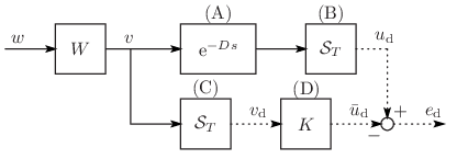
$W$ is a stable continuous-time system with strictly proper transfer function $\hat{W}(s)$ that defines the frequency-domain characteristic of the original analog signal $v$. More precisely, we assume that the analog signal $v$ is in the following subspace of $L^{2}$:

Note that the signal subspace $WL^{2}$ is much wider than that of band-limited $L^{2}$ signals [42].

The upper path of the diagram in Fig. 2 is the ideal process of the fractional delay filter (the process (A) $\rightarrow$ (B) in Fig. 1); that is, the continuous-time signal $v$ is delayed by the continuous-time delay denoted by ${\mathrm{e}}^{-Ds}$ (we use the notation ${\mathrm{e}}^{-Ds}$, the transfer function of the $D$-delay system, as the system itself), and then sampled by the ideal sampler denoted by ${\mathcal{S}}_{T}$ with period $T>0$ to become an $\ell^{2}$ signal³³ 3 If $\hat{W}(s)$ is stable and strictly proper, the discrete-time signal $u_{\mathrm{d}}={\mathcal{S}}_{T}{\mathrm{e}}^{-Ds}v$ belongs to $\ell^{2}$. Otherwise, ${\mathcal{S}}_{T}$ is not a bounded operator on $L^{2}$; see [29, Section 9.3]. $u_{\mathrm{d}}:={\mathcal{S}}_{T}{\mathrm{e}}^{-Ds}v$, or

On the other hand, the lower path represents the real process ((C) $\rightarrow$ (D) in Fig. 1); that is, the continuous-time signal $v$ is directly sampled with the same period $T$ to produce a discrete-time signal $v_{\mathrm{d}}\in\ell^{2}$ defined by

This signal is then filtered by a digital filter $K$ to be designed, and we obtain an estimation signal $\bar{u}_{\mathrm{d}}=K{\mathcal{S}}_{T}v\in\ell^{2}$.

Put $e_{\mathrm{d}}:=u_{\mathrm{d}}-\bar{u}_{\mathrm{d}}$ (the difference between the ideal output $u_{\mathrm{d}}$ and the estimation $\bar{u}_{\mathrm{d}}$), and let ${E}$ denote the error system from $w\in L^{2}$ to $e_{\mathrm{d}}\in\ell^{2}$ (see Fig. 2). Symbolically, ${E}$ is represented by (cf. (4))

Then our problem is to find a digital filter $K$ that minimizes the $H^{\infty}$ norm of the error system ${E}$.

Note that $W$, or its transfer function $\hat{W}(s)$, can be interpreted as a frequency-domain weighting function for the optimization. This is comparable to $\hat{W}_{\mathrm{d}}(z)$ in the discrete-time $H^{2}$ design minimizing (5). The point to use continuous-time $\hat{W}(s)$ is that one can model the frequency characteristic of signals beyond the Nyquist frequency. Also, the advantage of using the sampled-data setup here is that we can minimize the norm of the overall transfer operator from continuous-time $w$ to the error $e_{\rm d}$. In the next section, we will show a procedure to solve Problem 1 based on sampled-data control theory.

Let $\{{\boldsymbol{A}},{\boldsymbol{B}},{\boldsymbol{C}}\}$ be a minimal realization [43] of $\hat{W}(s)$:

where ${\boldsymbol{x}}(t)\in\mathbb{R}^{\nu}$ is the state variable ($\nu$ is a positive integer). We assume ${\boldsymbol{A}}\in\mathbb{R}^{\nu\times\nu}$, ${\boldsymbol{B}}\in\mathbb{R}^{\nu\times 1}$, ${\boldsymbol{C}}\in\mathbb{R}^{1\times\nu}$, and ${\boldsymbol{x}}(0)={\boldsymbol{0}}$. Let $D=mT+d$ where $m\in\mathbb{Z}_{+}$ and $d$ is a real number such that $0\leq d<T$. First, we introduce the lifting operator $\mathcal{L}$ [37, 29] that transforms a continuous-time signal in $L^{2}[0,\infty)$ to an $\ell^{2}$ sequence of functions in $L^{2}[0,T)$. Apply $\mathcal{L}$ to the continuous-time signals $w$ and $v$, and put $\widetilde{w}:=\mathcal{L}w$, $\widetilde{v}:=\mathcal{L}v$. By this, the error system in Fig. 2, is transformed into a time-invariant discrete-time system $\mathcal{E}$ shown in Fig. 3. Since the operator $\mathcal{L}$ gives an isometry between $L^{2}[0,\infty)$ and ${\tilde{\ell}}^{2}:=\ell^{2}(\mathbb{Z}_{+},L^{2}[0,T))$, we have

The following proposition is fundamental to the sampled-data optimization in (8).

The lifted system $\mathcal{E}$ given in (9), or its transfer function $\hat{\mathcal{E}}$ in (11), involves an infinite-dimensional operator ${\mathcal{B}}:L^{2}[0,T)\rightarrow\mathbb{R}^{\nu+1}$. Introducing the dual operator [44] ${\mathcal{B}}^{\ast}:\mathbb{R}^{\nu+1}\rightarrow L^{2}[0,T)$ of ${\mathcal{B}}$, and composing this with ${\mathcal{B}}$, we can obtain a norm-equivalent finite dimensional system of the infinite-dimensional system $\mathcal{E}$.

The dual operator ${\mathcal{B}}^{\ast}$ of ${\mathcal{B}}$ is given by [44]

where ${\boldsymbol{1}}_{[0,T-d)}$ is the characteristic function of the interval $[0,T-d)$, that is,

Then we have the following lemma:

Assume that the weighting function $\hat{W}(s)$ is a first-order low-pass filter with cutoff frequency $\omega_{\mathrm{c}}>0$:

Under this assumption, a closed-form solution for the optimal filter is obtained [31, 32]:

Since the optimal filter $\hat{K}(z)$ in (16) is a function of the fractional delay $d$ and the integer delay $m$, the filter can be used as a variable fractional delay filter [10].

References

- [1] T. A. Ramstad, “Digital methods for conversion between arbitrary sampling frequencies,” IEEE Trans. Acoust., Speech, Signal Processing, vol. 32, no. 3, pp. 577–591, 1984.
- [2] J. O. Smith and P. Gossett, “A flexible sampling-rate conversion method,” in IEEE ICASSP’84, 1984, pp. 19.4.1–19.4.4.
- [3] S. Park, G. Hillman, and R. Robles, “A novel structure for real-time digital sample-rate converters with finite precision error analysis,” in IEEE ICASSP’91, 1991, pp. 3613–3616.
- [4] H. Johansson and P. Löwenborg, “Reconstruction of nonuniformly sampled bandlimited signals by means of digital fractional delay filters,” IEEE Trans. Signal Processing, vol. 50, no. 11, pp. 2757 – 2767, Nov. 2002.
- [5] R. Prendergast, B. Levy, and P. Hurst, “Reconstruction of band-limited periodic nonuniformly sampled signals through multirate filter banks,” IEEE Trans. Circuits Syst. I, vol. 51, no. 8, pp. 1612–1622, Aug. 2004.
- [6] R. Yu, “Characterization and sampled-data design of dual-tree filter banks for Hilbert transform pairs of wavelet bases,” IEEE Trans. Signal Processing, vol. 55, no. 6, pp. 2458 –2471, Jun. 2007.
- [7] B. Dumitrescu, “SDP approximation of a fractional delay and the design of dual-tree complex wavelet transform,” IEEE Trans. Signal Processing, vol. 56, no. 9, pp. 4255 –4262, Sep. 2008.
- [8] V. V. H.-M. Lehtonen and T. I. Laakso, “Musical signal analysis using fractional-delay inverse comb filters,” in Proc. of the 10th Int. Conf. on Digital Audio Effects, Sep. 2007, pp. 261–268.
- [9] V. Välimäki, J. Pakarinen, C. Erkut, and M. Karjalainen, “Discrete-time modelling of musical instruments,” Rep. Prog. Phys, vol. 69, no. 1, pp. 1–78, 2006.
- [10] T. I. Laakso, V. Välimäki, M. Karjalainen, and U. K. Laine, “Splitting the unit delay,” IEEE Signal Processing Mag., vol. 13, pp. 30–60, 1996.
- [11] V. Välimäki and T. I. Laakso, “Principles of fractional delay filters,” in IEEE ICASSP’00, 2000, pp. 3870–3873.
- [12] V. Välimäki and T. I. Laakso, “Fractional delay filters — design and applications,” in Nonuniform Sampling. New York: Kluwer Academic/Plenum Publishers, 2001, pp. 835–885.
- [13] C. E. Shannon, “Communication in the presence of noise,” Proc. IRE, vol. 37, no. 1, pp. 10–21, 1949.
- [14] M. Unser, “Sampling — 50 years after Shannon,” Proc. IEEE, vol. 88, no. 4, 2000.
- [15] G. D. Cain, A. Yardim, and P. Henry, “Offset windowing for FIR fractional-sample delay,” in IEEE ICASSP’95, 1995, pp. 1276–1279.
- [16] J. Selva, “An efficient structure for the design of variable fractional delay filters based on the windowing method,” IEEE Trans. Signal Processing, vol. 56, no. 8, pp. 3770 –3775, Aug. 2008.
- [17] E. Hermanowicz, “Explicit formulas for weighting coefficients of maximally flat tunable FIR delayers,” Electronics Letters, vol. 28, pp. 1936–1937, 1992.
- [18] S.-C. Pei and P.-H. Wang, “Closed-form design of maximally flat FIR Hilbert transformers, differentiators, and fractional delayers by power series expansion,” IEEE Trans. Circuits Syst. I, vol. 48, pp. 389–398, 2001.
- [19] S. Samadi, O. Ahmad, and M. N. S. Swamy, “Results on maximally flat fractional-delay systems,” IEEE Trans. Circuits Syst. I, vol. 51, no. 11, pp. 2271–2286, 2004.
- [20] H. Hachabiboglu, B. Gunel, and A. Kondoz, “Analysis of root displacement interpolation method for tunable allpass fractional-delay filters,” IEEE Trans. Signal Processing, vol. 55, no. 10, pp. 4896 –4906, Oct. 2007.
- [21] J.-J. Shyu and S.-C. Pei, “A generalized approach to the design of variable fractional-delay FIR digital filters,” Signal Processing, vol. 88, no. 6, pp. 1428–1435, Jun. 2008.
- [22] Z. Jing, “A new method for digital all-pass filter design,” IEEE Trans. Acoust., Speech, Signal Processing, vol. 35, pp. 1557–1564, 1987.
- [23] S.-C. Pei and P.-H. Wang, “Closed-form design of all-pass fractional delay filters,” IEEE Signal Processing Lett., vol. 11, pp. 788–791, 2004.
- [24] W. Putnam and J. Smith, “Design of fractional delay filters using convex optimization,” in Applications of Signal Processing to Audio and Acoustics, 1997 IEEE ASSP Workshop on, Oct 1997.
- [25] A. Tarczynski, G. D. Cain, E. Hermanowicz, and M. Rojewski, “WLS design of variable frequency response FIR filters,” in Proc. IEEE Int. Symp. Circuits Syst., 1997, pp. 2244–2247.
- [26] T.-B. Deng and Y. Nakagawa, “SVD-based design and new structures for variable fractional-delay digital filters,” IEEE Trans. Signal Processing, vol. 52, pp. 2513–2527, 1991.
- [27] Y. Yamamoto, M. Nagahara, and P. P. Khargonekar, “Signal reconstruction via sampled-data control theory — Beyond the Shannon paradigm,” IEEE Trans. Signal Processing, vol. 60, no. 2, pp. 613–625, 2012.
- [28] P. P. Khargonekar and Y. Yamamoto, “Delayed signal reconstruction using sampled-data control,” in Proc. 35th IEEE CDC, 1996, pp. 1259–1263.
- [29] T. Chen and B. A. Francis, Optimal Sampled-data Control Systems. Springer, 1995.
- [30] J. C. Doyle, K. Glover, P. P. Khargonekar, and B. A. Francis, “State-space solutions to standard and control problems,” IEEE Trans. Automat. Contr., vol. 34, pp. 831–847, 1989.
- [31] M. Nagahara and Y. Yamamoto, “Optimal design of fractional delay filters,” in Proc. of 35th Conf. on Decision and Control, 2003, pp. 6539–6544.
- [32] M. Nagahara and Y. Yamamoto, “Optimal design of fractional delay FIR filters without band-limiting assumption,” in IEEE ICASSP’05, 2005, pp. 221–224.
- [33] Y. Yamamoto, “New approach to sampled-data systems: a function space method,” in Proc. 29th Conf. on Decision and Control, 1990, pp. 1881–1887.
- [34] B. Bamieh, J. B. Pearson, B. A. Francis, and A. Tannenbaum, “A lifting technique for linear periodic systems with applications to sampled-data control systems,” Syst. Control Lett., vol. 17, pp. 79–88, 1991.
- [35] H. T. Toivonen, “Sampled-data control of continuous-time systems with an optimality criterion,” Automatica, vol. 28, pp. 45–54, 1992.
- [36] B. Bamieh and J. B. Pearson, “A general framework for linear periodic systems with applications to sampled-data control,” IEEE Trans. Automat. Contr., vol. 37, pp. 418–435, 1992.
- [37] Y. Yamamoto, “A function space approach to sampled-data control systems and tracking problems,” IEEE Trans. Automat. Contr., vol. 39, pp. 703–712, 1994.
- [38] P. P. Vaidyanathan, Multirate Systems and Filter Banks. Prentice Hall, 1993.
- [39] G. Balas, R. Chiang, A. Packard, and M. Safonov, Robust Control Toolbox, Version 3. The Math Works, 2005.
- [40] C. W. Farrow, “A continuously variable digital delay element,” in Proc. IEEE Int. Symp. Circuits Syst., vol. 3, 1988, pp. 2641–2645.
- [41] N. J. Fliege, Multirate Digital Signal Processing. New York: John Wiley, 1994.
- [42] M. Nagahara, M. Ogura, and Y. Yamamoto, “ design of periodically nonuniform interpolation and decimation for non-band-limited signals,” SICE Journal of Control, Measurement, and System Integration, vol. 4, no. 5, pp. 341–348, 2011.
- [43] W. J. Rugh, Linear Systems Theory. Prentice Hall, 1996.
- [44] Y. Yamamoto, “On the state space and frequency domain characterization of -norm of sampled-data systems,” Syst. Control Lett., vol. 21, pp. 163–172, 1993.
- [45] C. F. V. Loan, “Computing integrals involving the matrix exponential,” IEEE Trans. Automat. Contr., vol. 23, pp. 395–404, 1994.
- [46] http://www-ics.acs.i.kyoto-u.ac.jp/mat/fdf/.
- [47] M. Nagahara, “Min-max design of FIR digital filters by semidefinite programming,” in Applications of Digital Signal Processing. InTech, Nov. 2011.
- [48] L. Jackson, “A correction to impulse invariance,” IEEE Signal Processing Lett., vol. 7, no. 10, pp. 273–275, Oct. 2000.
- [49] D. Donoho, A. Maleki, and M. Shaharam, “Wavelab 850,” 2006.