TCP-Aware Backpressure Routing and Scheduling Thanks: This work was supported by NSF grant CNS-0915988, ONR grant N00014-12-1-0064, ARO Muri grant number W911NF-08-1-0238.

The backpressure routing and scheduling paradigm has emerged from the pioneering work [1], [2], which showed that, in wireless networks where nodes route and schedule packets based on queue backlog differences, one can stabilize the queues for any feasible traffic. This seminal idea has generated a lot of research interest. Moreover, it has been shown that backpressure can be combined with flow control to provide utility-optimal operation [3].

The strengths of these techniques have recently increased the interest in practical implementation of the backpressure framework over wireless networks as summarized in Section VI. One important practical problem that remains open, and is the focus of this paper, is the performance of backpressure with Transmission Control Protocol (TCP) flows.

TCP is the dominant transport protocol in the Internet today and is likely to remain so for the foreseeable future. Therefore, it is crucial to exploit throughput improvement potential of backpressure routing and scheduling for TCP flows. However, TCP flows are not compatible with backpressure. Their joint behavior is so detrimental that some flows may never get a chance to transmit. To better illustrate this point, we first discuss the operation of backpressure in the following example.

The fundamental goal of TCP, which applies to all TCP variants, is to achieve as much bandwidth as possible while maintaining some level of long-term rate fairness across competing flows. By their very design, all TCP algorithms (both the widely employed loss-based versions and the delay-based ones) have their own “clock”, which relies on end-to-end acknowledgement (ACK) packets. Based on the received ACKs, TCP determines whether and how many packets should be injected into the network by updating its window size.

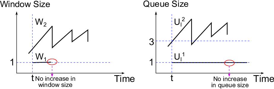
Example 1 - continued: Let us consider Fig. 1(b) to illustrate the interaction of backpressure and TCP. In Fig. 1(b), packet arrivals are controlled by TCP. Let us consider that loss-based TCP flavor, e.g., TCP-Reno or TCP-SACK, is employed. Assume that at time $t$, the TCP congestion window size of the first flow, i.e., $W_{1}(t)$, is small, e.g., $W_{1}(t)=1$ segment, (note that 1-segment window size may be seen at the beginning of a connection or after a re-transmit timeout), while the TCP congestion window size of the second flow is $W_{2}(t)>1$ (e.g., it may be the case that flow 2 has been transmitting for some time until $t$, and it has already increased its window size). As depicted in the figure, the example queue occupancies at time $t$ are $U_{I}^{1}(t)=1$ and $U_{I}^{2}(t)=3$. Since, $U_{I}^{2}(t)>U_{I}^{1}(t)$, a packet(s) from the second flow is transmitted. $R_{2}$ receives the transmitted packet, and passes it to TCP. TCP generates an ACK, and transmits it back to node $I$. TCP source of flow $2$ at node $I$ increases window size after receiving an ACK. Therefore, more packets are passed to $U_{I}^{2}(t)$. On the other hand, since $U_{I}^{1}(t)<U_{I}^{2}(t)$, no packets are transmitted from flow $1$. Thus, TCP does not receive any ACKs for the $1$st flow, does not increase its window size, and no (or sporadic) new packets are passed to $U_{I}^{1}(t)$. Eventually, the size of $U_{I}^{1}(t)$ almost never increases, so no packets are transmitted from flow $1$. Possible sample paths showing the evolution of $W_{1}$ and $W_{2}$ as well as $U_{I}^{1}$ and $U_{I}^{2}$ over time are shown in Fig. 2. As can be seen, the joint behavior of TCP and backpressure is so detrimental that flow $1$ does not get any chance to transmit. We confirm this observation via simulations in Section V. $\blacksquare$

The incompatibility of backpressure is not limited to the loss-based versions of TCP. The delay-based TCP flavors, e.g., TCP Vegas is also incompatible with backpressure, as TCP-Vegas has its own clock, which relies on end-to-end ACK packets to calculate round-trip-times (RTTs). If some packets are trapped in buffers due to backpressure as in the above example, sporadic or no ACK packets are received. This increases RTTs, and reduces end-to-end rate of TCP Vegas as there is inverse relationship between RTT and rate. Furthermore, backpressure leads to timeouts which reduce the end-to-end rate in both loss-based and delay-based TCP versions, including new TCP versions; TCP-Compound [4] and TCP-Cubic [5].

In this paper, we propose “TCP-aware backpressure” that helps TCP and backpressure operate in harmony. In particular, TCP-aware backpressure takes into account the behavior of TCP flows, and gives transmission opportunity to flows with short queues. This makes all TCP flows transmit their packets, so the TCP clock, which relies on packet transmissions and end-to-end ACKs, continues to operate. Furthermore, the throughput of TCP flows improves by exploiting the performance of the backpressure routing and scheduling. We note that backpressure introduces additional challenges when combined with TCP such as out of order delivery, high jitter RTTs, and packet losses due to corruption over wireless links. However, these challenges are not specific to backpressure, and exist when a multiple path routing scheme over wireless networks is combined with TCP. We address these challenges by employing network coding (in Section IV). Yet, the main focus of this paper is the incompatibility of TCP and backpressure and developing a TCP-aware backpressure framework. The following are the key contributions of this work:

• •

  We identify the mismatch between TCP and the backpressure framework; i.e., their joint behavior is so detrimental that some flows may never get a chance to transmit. In order to address the mismatch between TCP and backpressure, we develop “TCP-aware backpressure routing and scheduling”.

• •

  We show that (i) TCP-aware backpressure routing and scheduling stabilizes queues for any feasible traffic as the classical backpressure [1], [2], (ii) TCP-aware backpressure routing and scheduling provides the same utility-optimal operation guarantee when combined with a flow control algorithm as the classical backpressure [3].

• •

  We provide implementation details and explain how to tune TCP-aware backpressure in practice so that it complies with TCP. Moreover, we combine network coding and TCP-aware backpressure to address the additional challenges such as out of order delivery, packet loss, and jitter. Thanks to employing network coding, which makes TCP flows sequence agnostic (with respect to packet IDs), TCP-aware backpressure fully complies with TCP.

• •

  We evaluate our schemes in a multi-hop setting, using ns-2 [6]. The simulation results (i) confirm the mismatch of TCP and backpressure, (ii) show that TCP-aware backpressure is compatible with TCP, and significantly improves throughput as compared to existing adaptive routing schemes, (iii) demonstrate that TCP-aware backpressure provides fairness across competing TCP flows.

The structure of the rest of the paper is as follows. Section II gives an overview of the system model. Section III presents TCP-aware backpressure design and analysis. Section IV presents the implementation details of TCP-aware backpressure as well as its interaction with TCP. Section V presents simulation results. Section VI presents related work. Section VII concludes the paper.

We consider a general network model presented in Fig. 3, where flows may originate from a source in the Internet and traverse multiple hops to reach their destination in a wireless network. An end-to-end TCP connection is set up for each flow. Our goal in this paper is to develop TCP-aware backpressure routing and scheduling algorithms that operate in the wireless network. In this direction, we first develop our algorithms using the Lyapunov optimization framework (which is presented in Section III) by taking into account the incompatibility of TCP and classical backpressure. In this section, we provide an overview of the system model and assumptions that we use to develop the TCP-aware backpressure. Note that the interaction and implementation of TCP-aware backpressure routing and scheduling with actual TCP flows are presented in Section IV.

Wireless Network Setup: The wireless network consists of $N$ nodes and $L$ links, where $\mathcal{N}$ is the set of nodes and $\mathcal{L}$ is the set of links in the network. In this setup, each wireless node is able to perform routing and scheduling. Let $\mathcal{S}$ be the set of unicast flows between source-destination pairs in the network.We consider in our formulation and analysis that time is slotted, and $t$ refers to the beginning of slot $t$.

Channel Model: At slot $t$, $\boldsymbol{C}(t)$ $=\{C_{1}(t),$ $...,$ $C_{l}(t),$ $...,C_{L}(t)\}$ is the channel state vector, where $l$ represents the edges such that $l=(i,j)$, $(i,j)\in\mathcal{L}$ and $i\neq j$. For the sake of analysis, we assume that $C_{l}(t)$ is the state of link $l$ at time $t$ and takes values from the set $\{ON,OFF\}$ according to a probability distribution which is i.i.d. over time slots. If $C_{l}(t)=ON$, packets can be transmitted with rate $R_{l}$. Otherwise; (i.e., if $C_{l}(t)=OFF$), no packets are transmitted. Note that our analysis can be extended to more general channel state models [7]. We also consider a Rayleigh fading model in our simulations.

Let $\Gamma_{\boldsymbol{C}(t)}$ denote the set of the link transmission rates feasible at time slot $t$ and for channel state $\boldsymbol{C}(t)$ and interference among wireless links. In particular, at every time slot $t$, the link transmission vector $\boldsymbol{f}(t)=\{f_{1}(t),...,f_{l}(t),...f_{L}(t)\}$ should be constrained such that $\boldsymbol{f}(t)$ $\in\Gamma_{\boldsymbol{C}(t)}$. Hence, $f_{l}(t)$ takes a value from the set $\{R_{l},0\}$ depending on the channel state and interference among multiple wireless nodes. Also note that $\boldsymbol{f}(t)$ is determined by the scheduling algorithm.

Stability Region: Let $(\lambda_{s})$ be the vector of arrival rates $\forall s\in\mathcal{S}$. The network stability region $\Lambda$ is defined as the closure of all arrival rate vectors that can be stably transmitted in the network, considering all possible routing and scheduling policies [1], [2], [3]. $\Lambda$ is fixed and depends only on channel statistics and interference.

Flow Rates and Queue Evolution: Each flow $s\in\mathcal{S}$ is generated at its source node according to an arrival process $A_{s}(t)$, $\forall s\in\mathcal{S}$ at time slot $t$. The arrivals are i.i.d. over the slots and $\lambda_{s}=E[A_{s}(t)]$, $\forall s\in\mathcal{S}$. We assume that $E[A_{s}(t)]$ and $E[A_{s}(t)^{2}]$ are finite. Note that we make i.i.d. arrivals assumption for the purpose of designing and analyzing our algorithms in the Lyapunov optimization framework. This assumption is relaxed in the practical setup when we combine our algorithms with TCP flows in Section IV.

Each node $i$ constructs a per-flow queue $\mathcal{U}_{i}^{s}$ for each flow $s\in\mathcal{S}$. The size of the per-flow queue $\mathcal{U}_{i}^{s}$ at time $t$ is $U_{i}^{s}(t)$. Let $o(s)$ be the source node of flow $s$. The packets generated according to the arrival process $A_{s}(t)$ are inserted in the per-flow queue at node $o(s)$, i.e., in $\mathcal{U}_{o(s)}^{s}$. These queues only store packets from flow $s\in\mathcal{S}$. Each node $i$ such that $i\in\mathcal{N}$ and $i\neq o(s)$, may receive packets from its neighboring nodes and insert them in $\mathcal{U}_{i}^{s}$. The transmission rate of flow $s$ from node $i$ to node $j$ is $f_{i,j}^{s}(t)$. Since the link transmission rate over link $(i,j)$ is $f_{i,j}(t)$ at time $t$, multiple flows could share the available rate, i.e., $\sum_{s\in\mathcal{S}}f_{i,j}^{s}(t)\leq f_{i,j}(t)$. Accordingly, at every time slot $t$, the size of per-flow queues, i.e., $U_{i}^{s}(t)$ evolves according to the following dynamics.

		$\displaystyle U_{i}^{s}(t+1)\leq\max[U_{i}^{s}(t)-\sum_{j\in\mathcal{N}}f_{i,j}^{s}(t),0]+\sum_{j\in\mathcal{N}}f_{j,i}^{s}(t)$
		$\displaystyle+A_{s}(t)1_{[i=o(s)]},$		(1)

where $1_{[i=o(s)]}$ is an indicator function, which is $1$ if $i=o(s)$, and $0$, otherwise. Note that Eq. (1) is inequality, because the number of packets in the queue $U_{j}^{s}(t)$ may be less than $f_{j,i}^{s}(t)$.

In this section, we design and analyze the TCP-aware backpressure scheme. In particular, we provide a stochastic control strategy including routing and scheduling to address the incompatibility between TCP and classical backpressure.

TCP-Aware Backpressure:

• •

  Routing & Intra-Node Scheduling. The routing & intra-node scheduling part of TCP-aware backpressure determines a flow $s$ from which packets should be transmitted at slot $t$ from node $i$, as well as the next hop node $j$ to which packets from flow $s$ should be forwarded. The algorithm works as follows.

  Node $i$ observes per-flow queue backlogs in all neighboring nodes at time $t$, and determines queue backlog difference according to:

  $\displaystyle D_{i,j}^{s}(t)=\max\{K,U_{i}^{s}(t)\}-U_{j}^{s}(t),$

  (2)

  where $K$ is a non-negative finite constant. Let $l=(i,j)$ s.t. $j\in\mathcal{N}$ and $j\neq i$. The maximum queue backlog difference among all flows over link $l\in\mathcal{L}$ is;

  $\displaystyle D_{l}^{*}(t)=\max_{[s\in\mathcal{S}|l\in\mathcal{L}_{s}]}\{D_{l}^{s}(t)\}.$

  (3)

  The flow that maximizes the queue backlog differences over link $l$ is $s_{l}^{*}(t)$ and expressed as;

  $\displaystyle s_{l}^{*}(t)=\argmax_{[s\in\mathcal{S}|l\in\mathcal{L}_{s}]}\{D_{l}^{s}(t)\}.$

  (4)

  At time slot $t$, one or more packets are selected from the queue $\mathcal{U}_{i}^{s_{l}^{*}(t)}$ if $D_{l}^{*}(t)$ $>$ $0$ and $\mathcal{U}_{i}^{s_{l}^{*}(t)}$ has enough packets for transmission. The transmission of the selected packets depends on the channel conditions and interference constraints, and determined by inter-node scheduling.

  Note that TCP-aware backpressure uses queue backlog difference $\max\{K,U_{i}^{s}(t)\}-U_{j}^{s}(t)$ in Eq. (2) instead of $U_{i}^{s}(t)-U_{j}^{s}(t)$ in the classical backpressure. The advantage of using Eq. (2) in TCP-aware backpressure is that node $i$ may select packets from flow $s$ even if queue size $U_{i}^{s}(t)$ is small.¹¹ 1 Note that place-holder backlogs, such as using $U_{i}^{s}(t)+K$ instead of $U_{i}^{s}(t)$ has been considered in the literature [7]. Although place-holder algorithms are beneficial to improve end-to-end delay, they do not solve the problem we consider in this paper as they do not give transmission opportunity to small queues. This advantage is clarified through an illustrative example later in this section.

• •

  Inter-Node Scheduling. The inter-node scheduling (as also called resource allocation [3]) part of TCP-aware backpressure determines link transmission rates considering the link state information and interference constraints.

  Each node $i$ observes the channel state $\boldsymbol{C}(t)$ at time $t$, and determines a transmission vector $\boldsymbol{f}(t)=\{f_{1}(t),...,$ $f_{l}(t),...f_{L}(t)\}$ by maximizing $\sum_{l\in\mathcal{L}}D_{l}^{*}(t)f_{l}(t)$. Note that $\boldsymbol{f}(t)$ should be constrained such that $\boldsymbol{f}(t)\in\Gamma_{\boldsymbol{C}(t)}$, i.e., interference among multiple nodes should be taken into account. The resulting transmission rate $f_{l}(t)$ is used to transmit packets of flow $s_{l}^{*}(t)$ over link $l$.

Proof: The proof is provided in Appendix A. $\blacksquare$

Note that we propose TCP-aware backpressure; its routing, intra-node scheduling, and inter-node scheduling parts to work with TCP and TCP’s end-to-end flow control mechanism. In the next section, we provide implementation details. However, TCP-aware backpressure can also be combined with flow control schemes other than TCP’s, which is important for two reasons: (i) it may be possible or preferable to use personalized flow control mechanisms instead of TCP’s in some systems, (ii) there may be both TCP and non-TCP flows in some systems, where a TCP-friendly flow control mechanism combined with non-TCP flows is crucial to accommodate both TCP and non-TCP flows. We consider the following flow control algorithm, developed in [3], to complement TCP-aware backpressure for non-TCP flows.

The flow control algorithm at node $i$ determines the number of packets from flow $s$ that should be passed to the per-flow queues; $\mathcal{U}_{i}^{s}$ at every time slot $t$ according to;

	$\displaystyle\max_{\boldsymbol{x}}$	$\displaystyle\sum_{[s\in\mathcal{S}|i=o(s)]}[Mg_{s}(x_{s}(t))-U_{i}^{s}(t)x_{s}(t)]$
	s.t.	$\displaystyle\sum_{[s\in\mathcal{S}|i=o(s)]}x_{s}(t)\leq R_{i}^{max}$		(5)

where $R_{i}^{max}$ is a constant larger than the maximum outgoing rate from node $i$, $M$ is a positive constant, $x_{s}(t)$ is the rate of packets that will be inserted to the per-flow queue $\mathcal{U}_{i}^{s}$, and $g_{s}(.)$ is the utility function of flow $s$.

Proof: The proof of Theorem 2 directly follows when Appendix A and drif+penalty approach [3] are combined. $\blacksquare$

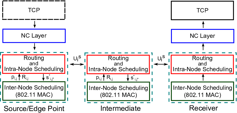
We present practical implementation details of TCP-aware backpressure as well as its interaction with different layers in the protocol stack (summarized in Fig. 4).

We simulate our scheme, TCP-aware backpressure (TCP-aware BP) as well as classical backpressure (classical BP), in ns-2 [6]. The simulation results; (i) confirm the mismatch of TCP and classical BP, (ii) show that TCP-aware BP is compatible with TCP, and significantly improves throughput as compared to existing routing schemes such as Ad-hoc On-Demand Distance Vector (AODV) [19], (iii) demonstrate that TCP-aware BP provides fairness across competing TCP flows. Next, we present the simulator setup and results in detail.

Backpressure, a routing and scheduling framework over communication networks [1], [2] has generated a lot of research interest [7], mainly in wireless ad-hoc networks. It has also been shown that backpressure can be combined with flow control to provide utility-optimal operation guarantee [3], [21].

The strengths of backpressure have recently increased the interest on practical implementation of backpressure over wireless networks. Backpressure has been implemented over sensor networks [22] and wireless multi-hop networks [23]. The multi-receiver diversity has been explored in wireless networks using backpressure in [24]. The 802.11 compliant version of enhanced backpressure is evaluated in [25]. Backpressure routing and rate control for intermittently connected networks was developed in [26].

Backpressure routing and (max-weight) scheduling with TCP over wireless has been considered in the literature. At the link layer, [27], [28], propose, analyze, and evaluate link layer backpressure-based implementations with queue prioritization and congestion window size adjustment. The interaction of TCP with backpressure in [27] and [28] is handled by updating the TCP congestion window evolution mechanism. In particular, if the queue size (at the TCP source) increases, the window size is reduced, otherwise, the window size is increased. Multi-path TCP scheme is implemented over wireless mesh networks [29] for routing and scheduling packets using a backpressure based heuristic, which avoids incompatibility with TCP. Max-weight scheduling is updated in [30] to make decisions based only on MAC level queue size information. Although [30] considers window based flow control mechanism similar to TCP, it does not consider existing TCP flavors. The main differences in our work are: (i) we consider the incompatibility of TCP with backpressure, and develop TCP-aware backpressure framework to address the incompatibilities, (ii) TCP-aware backpressure provides the same stability and utility-optimal operation guarantees as classical backpressure, (iii) we do not make any changes at the TCP source, (iv) we employ network coding to gracefully combine TCP and TCP-aware backpressure.

Maximum weight matching (MWM) is a switch scheduling algorithm and has similar properties as the max-weight scheduling algorithm and backpressure. Similar to the backpressure, there is incompatibility between TCP and MWM [31], [32]. Yet, we consider backpressure routing and scheduling over wireless networks rather than switch scheduling, and we take a holistic approach to address this problem; i.e., we propose TCP-aware backpressure to make TCP and backpressure compatible.

We proposed TCP-aware backpressure routing and scheduling to address the incompatibility of TCP and backpressure while exploiting the performance of backpressure routing and scheduling over wireless networks. TCP-aware backpressure is developed by taking into account the behavior of TCP flows, and gracefully combines TCP and backpressure without making any changes to the TCP protocol. Simulations in ns-2 demonstrate that TCP-aware backpressure improves throughput of TCP flows significantly and provides fairness across competing TCP flows.

The proof of Theorem 1 directly follows from $(\gamma,\xi)$ (or $C$-) approximation in [33], [7]. We provide the proof in this section for completeness. Let ${\mathop{f}\limits^{\vbox to-0.5pt{\kern-2.0pt\hbox{\scriptsize*}\vss}}}_{i,j}^{s}(t)$ be the optimal decision when $D_{i,j}^{s}(t)=U_{i}^{s}(t)-U_{j}^{s}(t)$ in Eq. (2) (note that this is the classical backpressure), while $f_{i,j}^{s}(t)$ be the decision when $D_{i,j}^{s}(t)=\max\{K,U_{i}^{s}(t)\}-U_{j}^{s}(t)$. If the following inequality holds, the policy that makes decision based on $D_{i,j}^{s}(t)=\max\{K,U_{i}^{s}(t)\}-U_{j}^{s}(t)$ stabilizes the queues.

		$\displaystyle\sum_{(i,j)\in\mathcal{L}}\sum_{s\in\mathcal{S}}f_{i,j}^{s}(t)(U_{i}^{s}(t)-U_{j}^{s}(t))\geq\sum_{(i,j)\in\mathcal{L}}\sum_{s\in\mathcal{S}}{\mathop{f}\limits^{\vbox to-0.5pt{\kern-2.0pt\hbox{\scriptsize*}\vss}}}_{i,j}^{s}(t)(U_{i}^{s}(t)$
		$\displaystyle-U_{j}^{s}(t))-Z,$		(6)

where $Z$ is a finite constant. Let us first show that Eq. (6) holds. Consider the inequality; $\sum_{(i,j)\in\mathcal{L}}\sum_{s\in\mathcal{S}}(U_{i}^{s}(t)-U_{j}^{s}(t)){\mathop{f}\limits^{\vbox to-0.5pt{\kern-2.0pt\hbox{\scriptsize*}\vss}}}_{i,j}^{s}(t)\leq\sum_{(i,j)\in\mathcal{L}}\sum_{s\in\mathcal{S}}\max\{K,U_{i}^{s}(t)\}{\mathop{f}\limits^{\vbox to-0.5pt{\kern-2.0pt\hbox{\scriptsize*}\vss}}}_{i,j}^{s}(t)$. This inequality holds, because $\max\{K,U_{i}^{s}(t)\}$ $\geq$ $U_{i}^{s}(t)$. Also, considering that $f_{i,j}^{s}(t)$ is the optimal decision when the backlog difference is $\max\{K,U_{i}^{s}(t)\}-U_{j}^{s}(t)$, the term $(\max\{K,$ $U_{i}^{s}(t)\}$ $-U_{j}^{s}(t))f_{i,j}^{s}(t)$ should be greater than $(\max\{K,U_{i}^{s}(t)\}$ $-U_{j}^{s}(t))$ ${\mathop{f}\limits^{\vbox to-0.5pt{\kern-2.0pt\hbox{\scriptsize*}\vss}}}_{i,j}^{s}(t)$. Therefore, the inequality is expressed as; $\sum_{(i,j)\in\mathcal{L}}\sum_{s\in\mathcal{S}}(U_{i}^{s}(t)-U_{j}^{s}(t)){\mathop{f}\limits^{\vbox to-0.5pt{\kern-2.0pt\hbox{\scriptsize*}\vss}}}_{i,j}^{s}(t)\leq\sum_{(i,j)\in\mathcal{L}}\sum_{s\in\mathcal{S}}\max$ $\{K,U_{i}^{s}(t)\}f_{i,j}^{s}(t)$. By adding and removing terms, and noting that $\max\{K,U_{i}^{s}(t)\}-U_{i}^{s}(t)\leq K$ and $f_{i,j}^{s}(t)\leq F_{\max}$ such that $F_{\max}\geq R_{i,j}$, the following holds;

		$\displaystyle\sum_{(i,j)\in\mathcal{L}}\sum_{s\in\mathcal{S}}(U_{i}^{s}(t)-U_{j}^{s}(t))f_{i,j}^{s}(t)\geq\sum_{(i,j)\in\mathcal{L}}\sum_{s\in\mathcal{S}}(U_{i}^{s}(t)$
		$\displaystyle-U_{j}^{s}(t)){\mathop{f}\limits^{\vbox to-0.5pt{\kern-2.0pt\hbox{\scriptsize*}\vss}}}_{i,j}^{s}(t)-|\mathcal{L}||\mathcal{S}|KF_{\max}$		(7)

Eq. (7) verifies that Eq. (6) holds considering that $Z=$ $|\mathcal{L}|$ $|\mathcal{S}|$ $K$ $F_{\max}$. Note that Eq. (7) is equivalent to;

		$\displaystyle\sum_{i\in\mathcal{N}}\sum_{s\in\mathcal{S}}U_{i}^{s}(t)(\sum_{j\in\mathcal{N}}f_{i,j}^{s}(t)-\sum_{j\in\mathcal{N}}f_{j,i}^{s}(t))\geq\sum_{i\in\mathcal{N}}\sum_{s\in\mathcal{S}}U_{i}^{s}(t)$
		$\displaystyle(\sum_{j\in\mathcal{N}}{\mathop{f}\limits^{\vbox to-0.5pt{\kern-2.0pt\hbox{\scriptsize*}\vss}}}_{i,j}^{s}(t)-\sum_{j\in\mathcal{N}}{\mathop{f}\limits^{\vbox to-0.5pt{\kern-2.0pt\hbox{\scriptsize*}\vss}}}_{j,i}^{s}(t))-|\mathcal{L}||\mathcal{S}|KF_{\max}$		(8)

Now, let us define the Lyapunov function as; $L(\boldsymbol{U}(t))=\sum_{i\in\mathcal{N}}\sum_{s\in\mathcal{S}}U_{i}^{s}(t)^{2}$, where $\boldsymbol{U}(t)=\{U_{i}^{s}(t)\}_{i\in\mathcal{N},s\in\mathcal{S}}$ and $U_{i}^{s}(t)$ evolves according to Eq. (1). Let the Lyapunov drift be $\Delta(\boldsymbol{U}(t))=E[L(\boldsymbol{U}(t+1))-L(\boldsymbol{U}(t))|\boldsymbol{U}(t)]$, which is equal to $\Delta(\boldsymbol{U}(t))\leq E[\sum_{i\in\mathcal{N}}\sum_{s\in\mathcal{S}}(U_{i}^{s}(t+1))^{2}-\sum_{i\in\mathcal{N}}\sum_{s\in\mathcal{S}}$ $(U_{i}^{s}(t))^{2}|\boldsymbol{U}(t)]$. Using the fact that $(\max(Q-b,0)+A)^{2}\leq Q^{2}+A^{2}+b^{2}+2Q(A-b)$, we have; $\Delta(\boldsymbol{U}(t))\leq E[\sum_{i\in\mathcal{N}}\sum_{s\in\mathcal{S}}$ $(\sum_{j\in\mathcal{N}}f_{i,j}^{s}(t))^{2}+\sum_{i\in\mathcal{N}}\sum_{s\in\mathcal{S}}(\sum_{j\in\mathcal{N}}f_{i,j}^{s}(t)+A_{s}(t)1_{[i=o(s)]})^{2}$ $+\sum_{i\in\mathcal{N}}\sum_{s\in\mathcal{S}}2U_{i}^{s}(t)(\sum_{j\in\mathcal{N}}f_{j,i}^{s}(t)-\sum_{j\in\mathcal{N}}f_{i,j}^{s}(t))+\sum_{i\in\mathcal{N}}$ $\sum_{s\in\mathcal{S}}2U_{i}^{s}(t)A_{s}(t)1_{[i=o(s)]}|\boldsymbol{U}(t)]$. Noting that there always exist a finite constant $B$ such that $B\geq E[\sum_{i\in\mathcal{N}}\sum_{s\in\mathcal{S}}(\sum_{j\in\mathcal{N}}$ $f_{i,j}^{s}(t))^{2}+\sum_{i\in\mathcal{N}}\sum_{s\in\mathcal{S}}(\sum_{j\in\mathcal{N}}$ $f_{i,j}^{s}(t)+A_{s}(t)1_{[i=o(s)]})^{2}|\boldsymbol{U}(t)]$, we have;

	$\displaystyle\Delta(\boldsymbol{U}(t))$	$\displaystyle\leq B-2E[\sum_{i\in\mathcal{N}}\sum_{j\in\mathcal{N}}\sum_{s\in\mathcal{S}}U_{i}^{s}(t)(f_{i,j}^{s}(t)-f_{j,i}^{s}(t))$
		$\displaystyle+2\sum_{i\in\mathcal{N}}\sum_{s\in\mathcal{S}}U_{i}^{s}(t)A_{s}(t)1_{[i=o(s)]}|\boldsymbol{U}(t)]$		(9)

When we insert Eq. (8) in Eq. (9), we have

		$\displaystyle\Delta(\boldsymbol{U}(t))\leq B+2\sum_{i\in\mathcal{N}}\sum_{s\in\mathcal{S}}U_{i}^{s}(t)\lambda_{i}^{s}-2E[\sum_{i\in\mathcal{N}}\sum_{s\in\mathcal{S}}U_{i}^{s}(t)$
		$\displaystyle(\sum_{j\in\mathcal{N}}{\mathop{f}\limits^{\vbox to-0.5pt{\kern-2.0pt\hbox{\scriptsize*}\vss}}}_{i,j}^{s}(t)-\sum_{j\in\mathcal{N}}{\mathop{f}\limits^{\vbox to-0.5pt{\kern-2.0pt\hbox{\scriptsize*}\vss}}}_{j,i}^{s}(t))|\boldsymbol{U}(t)]+2|\mathcal{L}||\mathcal{S}|KF_{\max}$		(10)

If the vector of arrival rates are interior to the stability region, there always exist $\epsilon>0$ such that $E[\sum_{i\in\mathcal{N}}\sum_{s\in\mathcal{S}}$ $(\sum_{j\in\mathcal{N}}{\mathop{f}\limits^{\vbox to-0.5pt{\kern-2.0pt\hbox{\scriptsize*}\vss}}}_{j,i}^{s}(t)-\sum_{j\in\mathcal{N}}{\mathop{f}\limits^{\vbox to-0.5pt{\kern-2.0pt\hbox{\scriptsize*}\vss}}}_{i,j}^{s}(t))|\boldsymbol{U}(t)]\leq-(\lambda_{s}1_{[i=o(s)]}+\epsilon)$. Substituting this into Eq. (10);

$\displaystyle\Delta(\boldsymbol{U}(t))$

$\displaystyle\leq B+2|\mathcal{L}||\mathcal{S}|KF_{\max}-2\sum_{i\in\mathcal{N}}\sum_{s\in\mathcal{S}}U_{i}^{s}(t)\epsilon$

(11)

The time average of Eq. (11) yields;

$\displaystyle\limsup_{t\rightarrow\infty}\frac{1}{t}\sum_{\tau=0}^{t-1}\Delta(\boldsymbol{U}(\tau))\leq\frac{B+2|\mathcal{L}||\mathcal{S}|KF_{\max}}{2\epsilon}$

(12)

which shows that the time average of $U_{i}^{s}(t)$ is bounded. Thus, TCP-aware backpressure stabilizes the network and the total average backlog is bounded.

References

- [1] L. Tassiulas, A. Ephremides, “Stability properties of constrained queueing systems and scheduling policies for maximum throughput in multihop radio networks,” in IEEE Trans. on Auto. Control, vol. 37(12), Dec. 1992.
- [2] L. Tassiulas, A. Ephremides, “Dynamic server allocation to parallel queues with randomly varying connectivity,” in IEEE ToIT, vol. 39(2), March 1993.
- [3] M. J. Neely, E. Modiano, C. Li, “Fairness and optimal stochastic control for heterogeneous networks,” in IEEE/ACM ToN, vol. 16(2), April 2008.
- [4] K. Tan,J. Song, Q. Zhang, M. Sridharan, “A compound TCP approach for high-speed and long distance networks,” in Proc. of IEEE INFOCOM, Barcelona, Spain, April 2006.
- [5] S. Ha, I. Rhee, L. Xu, “CUBIC: a new TCP-friendly high-speed TCP variant,” in SIGOPS Oper. Syst. Rev., vol. 42(5), July 2008.
- [6] The Network Simulator - ns-2, Version 2.35, available at www.isi.edu/nsnam/ns/.
- [7] M. J. Neely, “Stochastic network optimization with application to communication and queueing systems,” Morgan & Claypool, 2010.
- [8] H. Seferoglu, E. Modiano, “TCP-aware backpressure routing and scheduling,” Tech. Report, available at newport.eecs.uci.edu/~hseferog/, http://www.mit.edu/~hseferog/.
- [9] M. Chiang, S. T. Low, A. R. Calderbank, J. C. Doyle, “Layering as optimization decomposition: a mathematical theory of network architectures,” in Proceedings of the IEEE, vol. 95(1), Jan. 2007.
- [10] X. Lin, N. B. Schroff, R. Srikant, “A tutorial on cross-layer optimization in wireless networks,” in IEEE JSAC, vol. 24(8), Aug. 2006.
- [11] H. Seferoglu, E. Modiano, “Diff-Max: separation of routing and scheduling in backpressure-based wireless Networks,” in Proc. of IEEE INFOFOCM, Turin, Italy, April, 2013.
- [12] L. X. Bui, R. Srikant, A. Stolyar, “A novel architecture for reduction of delay and queueing structure complexity in the back-pressure algorithm,” in IEEE/ACM Transactions on Networking, vol. 19(6), Dec. 2011.
- [13] J. K. Sundararajan, D. Shah, M. Medard, M. Mitzenmacher, J. Barros, “Network coding meets TCP,” in Proc. of IEEE INFOCOM, Rio de Janeiro, Brazil, April 2009.
- [14] S. Gheorghiu, A. L. Toledo, P. Rodriguez, “Multi-path TCP with network coding for wireless mesh networks,” in Proc. of IEEE ICC, Cape Town, South Africa, May 2010.
- [15] H. Seferoglu, A. Markopoulou, K. K. Ramakrishnan, “I2NC: intra- and inter-session network coding for unicast flows in wireless networks,” in Proc. of IEEE INFOCOM, Shanghai, China, April 2011.
- [16] P. A. Chou, Y. Wu,“Network coding for the Internet and wireless networks,” in IEEE Signal Proc. Magazine, vol. 24(5), Sept. 2007.
- [17] J. Padhye, V. Firoiu, D. Towsley, J. Kurose, “Modeling TCP throughput: a simple model and its empirical validation,” in Proc. of ACM SIGCOMM, Vancouver, Canada, Sep. 1998.
- [18] S. Low, “A duality model of TCP and queue management algorithms,” in IEEE/ACM Transactions on Networking, vol. 11(4), Aug. 2003.
- [19] C. Perkins, E. Belding-Royer, S. Das, “Ad hoc on-demand distance vector (AODV) routing,” RFC 3561, IETF, July 2003.
- [20] R. K. Jain, “The art of computer systems performance analysis: techniques for experimental design, measurement, simulation, and modeling,” John Wiley & Sons, April 1991.
- [21] A. L. Stolyar, “Greedy primal dual algorithm for dynamic resource allocation in complex networks,” in Queuing Systems, vol. 54, 2006.
- [22] S. Moeller, A. Sridharan, B. Krishnamachari, O. Gnawali, “Routing without routes: the backpressure collection protocol,” in Proc. of ACM IPSN, Stockholm, Sweden, April 2010.
- [23] R. Laufer, T. Salonidis, H. Lundgren, P. L. Guyadec, “XPRESS: a cross-layer backpressure architecture for wireless multi-hop networks,” in Proc. of ACM MobiCom, Las Vegas, NV, Sep. 2011.
- [24] A. A. Bhorkar, T. Javidi, A. C. Snoereny, “Achieving congestion diversity in wireless ad-hoc networks,” in Proc. of IEEE INFOCOM, Shanghai, China, April 2011.
- [25] K. Choumas, T. Korakis, I. Koutsopoulos, L. Tassiulas, “Implementation and end-to-end throughput evaluation of an IEEE 802.11 compliant version of the enhanced-backpressure algorithm,” in Proc. of TridentCom, Thessaloniki, Greece, June 2012.
- [26] J. Ryu, V. Bhargava, N. Paine, S. Shakkottai, “Backpressure routing and rate control for ICNs,” in Proc. of ACM MobiCom, Chicago, IL, Sep. 2010.
- [27] A. Warrier, S. Janakiraman, S. Ha, I. Rhee, “DiffQ: practical differential backlog congestion control for wireless networks,” in Proc. of IEEE INFOCOM, Rio de Janerio, Brazil, April 2009.
- [28] U. Akyol, M. Andrews, P. Gupta, J. Hobby, I. Saniee, A. Stolyar, “Joint scheduling and congestion control in mobile ad-hoc networks,” in Proc. of IEEE INFOCOM, Phoenix, AZ, April 2008.
- [29] B. Radunovic, C. Gkantsidis, D. Gunawardena, P. Key, “Horizon: balancing TCP over multiple paths in wireless mesh network,” in Proc. of ACM MobiCom, San Francisco, CA, Sep. 2008.
- [30] J. Ghaderi, T. Ji, R. Srikant, “Connection-level scheduling in wireless networks using only MAC-layer information,” in Proc. of IEEE INFOCOM, Orlando, FL, March 2012.
- [31] A. Shpiner, I. Keslassy, “Modeling the interactions of congestion control and switch scheduling,” in Computer Networks, vol. 55(6), April 2011.
- [32] P. Giaccone, E. Leonardi, F. Neri, “On the interaction between TCP-like sources and throughput-efficient scheduling policies,” in Elsevier, 2013.
- [33] Y. Yi, A. Proutière, and M. Chiang, “Complexity in wireless scheduling: impact and tradeoffs,” in Proc. of ACM MobiHoc, Hong Kong, China, May 2008.
Appendix A: Proof of Theorem 1
The proof of Theorem 1 directly follows from (or -) approximation in [33], [7]. We provide the proof in this section for completeness. Let be the optimal decision when in Eq. (2) (note that this is the classical backpressure), while be the decision when . If the following inequality holds, the policy that makes decision based on stabilizes the queues.