11.5pt
Abstract
The dijet double-differential cross section is measured as a function of the dijet invariant mass, using data taken during 2010 and during 2011 with the ATLAS experiment at the LHC, with a center-of-mass energy, . The measurements are sensitive to invariant masses between and 4.27 TeV with center-of-mass jet rapidities up to 3.5. A novel technique to correct jets for pile-up (additional proton-proton collisions) in the 2011 data is developed and subsequently used in the measurement. The data are found to be consistent over 12 orders of magnitude with fixed-order NLO pQCD predictions provided by NLOJET++. The results constitute a stringent test of pQCD, in an energy regime previously unexplored.
The dijet analysis is a confidence building step for the extraction of the signal of hard double parton scattering in four-jet events, and subsequent extraction of the effective overlap area between the interacting protons, expressed in terms of the variable, . The measurement of double parton scattering is performed using the 2010 ATLAS data. The rate of double parton scattering events is estimated using a neural network. A clear signal is observed, under the assumption that the double parton scattering signal can be represented by a random combination of exclusive dijet production. The fraction of double parton scattering candidate events is determined to be in the analyzed phase-space of four-jet topologies. Combined with the measurement of the dijet and four-jet cross sections in the appropriate phase-space regions, the effective cross section is found to be . This result is consistent within the quoted uncertainties with previous measurements of at center-of-mass energies between 63 GeV and 7 TeV, using several final states.
Acknowledgements
It is with immense gratitude that I acknowledge my supervisors, Prof. Halina Abramowicz and Prof. Aharon Levy, not only for teaching me physics, but for making me feel like part of the family. This thesis is a tribute to their steadfast encouragement, guidance and support, making the course of my studies a pleasure which is difficult to leave behind. I could not have hoped for a better pair of physicists, or for a more caring pair of people, to be a student of.
I consider it an honor to have worked on the double parton scattering analysis with my colleague and friend, Orel Gueta. Defeats and victories, late night insights and countless discussions, have all culminated in a measurement to be proud of. Great thanks is also owed to Dr. Arthur Moraes, for inspiring us with his ideas about multiple interactions, and for keeping faith when all seemed lost. In addition, the shared experience of Dr. Frank Krauss and of Dr. Eleanor Dobson has been instrumental in the success of the analysis, and is much appreciated. On the theoretical side of things, the fruitful discussions with Prof. Yuri Dokshitzer, Prof. Mark Strikman, Prof. Leonid Frankfurt and Prof. Evgeny Levin were of great help in formulating the strategy of the analysis.
I would like to show special appreciation to Dr. Sven Menke and Dr. Teresa Barillari for the stimulating discussions on all things calorimeter (and then some), and to Prof. Allen Caldwell in addition. They have made my visits to the Max-Planck-Institut für Physik in Munich an experience to remember, intellectually and otherwise.
Several people have contributed greatly to my understanding of the workings of the ATLAS experiment, be it in terms of performance or of physics. The debates with Dr. Ariel Schwartzman and Dr. Peter Loch have been of great help in my development of a pile-up correction using the jet area/median method. To start me off on the invariant mass measurement, the guidance of Dr. Christopher Meyer via many hours of discussions and a multitude of emails, has been invaluable. I would like to thank Dr. Pavol Strizenec for starting me off on ATLAS software. I would also like to Acknowledge Dr. Eric Feng and Dr. Serguei Yanush, for developing the software framework for calculation of the non-perturbative corrections to the invariant mass theoretical predictions.
I am grateful to my colleagues and the members of the group at Tel Aviv University, Prof. Gideon Alexander, Prof. Erez Etzion, Prof. Abner Soffer, Dr. Gideon Bella, Dr. Sergey Kananov, Dr. Zhenya Gurvich, Dr. Ronen Ingbir, Amir Stern, Rina Schwartz and Itamar Levy, for allowing me to bounce ideas off of, for the stimulating discussions, and for the pleasure of their company.
Finally, completing this thesis would not have been possible without the love and support of my family. As with everything else which is good in my life, it all starts and ends with them. Thank you for being you.
Preface
The goal of this thesis is the study of double-parton scattering (DPS) in four-jet events with the ATLAS experiment. In order to extract DPS in this channel, a good understanding of the reconstruction and calibration of jets is needed. A comprehensive framework exists in ATLAS for this purpose, featuring two main calibration schemes, referred to as the electromagnetic (EM) and the local-hadron (LCW) calibrations. These rely on extensive test-beam and simulation campaigns, which are the result of the efforts of a large number of individual researchers and analysis subgroups.
Test-beam data taken during 2004 served to test the detector performance and to validate the description of the data by simulations. Due to changing software models, these data became incompatible with current ATLAS reconstruction tools. In order to maintain future access, the information had to be made persistent, i.e., compatible with all future software. The first project which had been undertaken by the author of this thesis in ATLAS, was persistification of the test-beam data. This was followed by continued support and maintenance of the ATLAS calorimeter reconstruction software, as part of the operational contribution of the author to the experiment.
One of the major challenges in the calibration of jets in ATLAS, is the existence of pile-up, additional proton-proton () collisions, which coincide with the hard scattering of interest. The effects of pile-up on final states which involve jets are complicated. Pile-up tends to both bias the energy of jets which originate from the hard interaction, and to introduce additional jets which originate from the extraneous collisions. The current pile-up subtraction method in ATLAS involves a simulation-based scheme; it affects an average correction for jet energies, based on the instantaneous luminosity and on the number of reconstructed vertices in an event. An alternate, event-by-event-based correction, has been developed by the author for the LCW calibration scheme. In the new correction, referred to as the jet area/median method, the area of a given jet and the “local” energy-density, are used in order to subtract pile-up energy from the jet. The method takes advantage both of the average response of the calorimeter to pile-up energy, and of the observed energy in the vicinity of the jet of interest. The median method is completely data-driven. Consequently, compared to the nominal pile-up correction, the uncertainties on the energy correction associated with the simulation of pile-up were reduced.
The new pile-up correction was developed by the author, initially by using the ATLAS detector simulation. It was subsequently validated by the author with the 2011 ATLAS dataset, in which the rate of pile-up is high. The validation included in-situ measurements of several observables, one of which was the invariant mass of dijets, the system of the two jets with the highest transverse momentum in an event. The author also performed measurements of the dijet double-differential cross section for different center-of-mass jet rapidities, as a function of the invariant mass of dijets. The invariant mass spectra had previously been measured in ATLAS using the 2010 data. The new measurements, performed for the first time on the 2011 data, were found to be compatible with the previous observations, showing that the pile-up corrections were under control. In addition, the measurement using the larger dataset recorded during 2011, served to extend the experimental reach to higher values of the invariant mass.
Using the improved jet calibration, events with four-jets in the final state were investigated as part of the DPS analysis. It was shown by the author that the deterioration of the energy resolution due to pile-up distorted greatly the observables of the measurement. The scope of the measurement had, therefore, to be limited. As this is a first measurement of double parton scattering in this channel in ATLAS, it was decided to choose a conservative approach and to limit the systematic uncertainties as much as possible. The analysis, therefore, used only single-vertex events from the 2010 dataset, for which pile-up corrections are small.
Several strategies of the DPS analysis were explored by the author. For instance, the author attempted to measure the fraction of DPS events, by exploiting the sum of the pair-wise transverse momentum balance between different jet-pair combinations in a four-jet event, as previously done by the CDF collaboration. The problem with this type of approach was the absence of an appropriate simulation sample, in which DPS events within the required phase-space were generated. In order to avoid dependence on simulated DPS events, and in addition, to increase the robustness of the analysis, the author decided to utilize a neural network. Two input samples were prepared by the author for the neural network. The first consisted of simulated events in which multiple-interactions were switched off. The second, which stood for the DPS signal, was comprised of overlaid simulated dijet events. Utilizing the neural network, the fraction of double parton scattering events was extracted from the data, and the effective cross section for DPS was subsequently measured. The result was found to be compatible with previous measurements which had used several final states, at center-of-mass energies between 63 GeV and 7 TeV.
Table of Contents
Chapter 1 Introduction
The Standard Model (SM) [1] is one of the major intellectual achievements of the twentieth century. In the late 1960s and early 1970s, decades of path breaking experiments culminated in the emergence of a comprehensive theory of particle physics. This theory identifies the fundamental constituents of matter and combines the theory of electromagnetic, weak and strong interactions.
Numerous measurements at energy scales from a few eV to several TeV are reproduced by the SM, and many of its predictions, e.g., the existence of the and bosons, have been found to be realised in nature. By now, only the source of electroweak symmetry breaking, which in the SM is attributed to the Higgs mechanism, has not been verified experimentally. A particle with properties consistent with those of the Higgs boson has recently been discovered at the LHC by the ATLAS [2] and CMS [3] experiments; the final piece of the puzzle is therefore within reach.
The Standard Model falls short of being a complete theory of fundamental interactions because it does not incorporate the full theory of gravitation, as described by general relativity; nor does it predict the accelerating expansion of the universe, as possibly described by dark energy. The theory does not contain any viable dark matter particle that possesses all of the required properties deduced from observational cosmology. It also does not correctly account for neutrino oscillations or for the non-zero neutrino masses. Although the SM is believed to be theoretically self-consistent, it has several apparently unnatural properties, giving rise to puzzles like the strong CP problem and the hierarchy problem [4]. The SM is therefore viewed as an effective field theory that is valid at the lower energy scales where measurements have been performed, but which arises from a more fundamental theory at higher scales. It is therefore expected that a more fundamental theory exists beyond the TeV energy scale that explains the missing features.
Verification of the Higgs mechanism and the search for new physics beyond the SM are two of the primary enterprises in particle physics today. Any experimental search for the Higgs boson or for new interactions or particles, requires a detailed understanding of the strong interactions, described by Quantum Chromodynamics (QCD). It is common to discuss high-energy phenomena involving QCD in terms of partons (quarks and gluons), yet partons are never visible in their own right. Almost immediately after being produced, a quark or gluon fragments and hadronizes, leading to a collimated spray of energetic hadrons, which may be characterized by a jet [5]. Since partons interact strongly, jet production is the dominant hard scattering process in the SM. Figure 1 shows the production cross section for various processes as a function of the center-of-mass energy of an accelerator.

One may compare the production cross section for energetic jets with transverse energy above , with those of other processes ( and ) involving leptons. At the center-of-mass energy of the LHC, the former is much larger than the latter.
Because of the large cross sections, jet production provides an ideal avenue to probe QCD and parton distribution functions [6, 7, 8, 9], which describe the distribution of the momenta of quarks and gluons within a proton. Processes involving jets also serve as large backgrounds in many searches for new physics. Many models predict the production of new heavy and coloured particles at the LHC. These particles are expected to decay into quarks and gluons, which are detected as particle jets. Such models may therefore be tested by measuring the rate of jet production and comparing it to the expectations from QCD [10]. Other models, such as quark compositeness (the hypothesis that quarks are composed of more fundamental particles), may be realised through contact interactions between quarks. Such new phenomena may be discovered by measuring the kinematic distributions of jets [11].
In the most common final state involving jets at the LHC, two jets with high transverse momentum, , emerge from the interaction, as illustrated in figure 2a. These dijet events are particularly useful for measuring quantities associated with the initial interaction, such as the polar scattering angle in the two-parton center-of-mass frame, and the dijet invariant mass. Precise tests of perturbative QCD (pQCD) at high energies, may therefore be carried out by comparing the theoretical predictions to the experimental distributions. In addition, new physics may manifest itself with e.g., the production of a new massive particle, which subsequently decays into a high-mass dijet system [12]. Final states composed of low- or forward jets are also interesting. These topologies are sensitive to QCD effects which can not be calculated using perturbation theory; as such, their measurement may help to improve the phenomenological models which are currently in use in this regime.


Event display of an event with four reconstructed jets, taken in April 2010. The four jets all have GeV, where the highest- jet has transverse momentum of 108 GeV. Depicted points-of-view are along the beam axis (left), parallel to the beam axis (top right), and the angular distribution of transverse energy in and (bottom right).
One of the important sources of background for physics searches at the LHC are multiple-parton interactions (MPI). In a generic hadron-hadron collision, several partons in one hadron scatter on counterparts from the other hadron. Most of these interactions are soft, and so generally do not result in high- jets. However, the kinematic reach of the LHC, which extends to high energies and low fractions of proton momenta, enhances the probability of hard MPI relative to past experiments [13]. Hard MPI constitute a source of background for e.g., Higgs production [14, 15], and can possibly influence observed rates of other final states, involving the decay of heavy objects. The existing phenomenology of MPI is based on several simplifying assumptions. Recent interest has produced some advancements [16, 17, 18, 19, 20, 21, 22], however, a systematic treatment within QCD remains to be developed.
The simplest case of MPI is that of double parton scattering (DPS). Measurements of DPS at energies between 63 GeV and 1.96 TeV in the four-jet and + three-jets channels have previously been performed [23, 24, 25, 26, 27]. In addition, a measurement using 7 TeV ATLAS data with + two-jet production in the final state has recently been released [28]. These have proven helpful in constraining the phenomenological models which describe DPS, and in the development of double parton distribution functions, as e.g., discussed in [17]. An additional channel in which DPS may be measured at the LHC is four-jet production. An ATLAS event display of a four-jet event is presented in figure 2b for illustration. A four-jet final state may arise due to a single parton-parton collision, accompanied by additional radiation. Alternatively, it can also originate from two separate parton-parton collisions, each producing a pair of jets. The latter case has distinguishing kinematic characteristics, and so the rate of DPS may be estimated on average. The DPS-rate is related to a so-called effective cross section. The latter holds information about the transverse momentum distributions of partons in the proton, and about the correlations between partons. A measurement of DPS in four-jet events has been performed using a sub-sample of the 2010 ATLAS dataset, and is presented in this thesis.
Outline of the thesis This thesis presents a measurement of hard double parton scattering in four-jet events. The analysis involves measurement of the dijet and four-jet cross sections, and the extraction of the rate of double parton scattering from the four-jet sample.
In order to measure the individual cross sections, a measurement of the inclusive dijet invariant mass distribution is first performed. Part of the experimental challenge of measurements involving jets in ATLAS, is the calibration of the energy of jets, as these suffer from detector background due to multiple simultaneous collisions, referred to as pile-up. A novel method to reduce the pile-up background using jet areas is developed and subsequently utilized to correct the energy of jets. The re-calibrated jets serve as input for the dijet mass distribution analysis of the 2011 ATLAS dataset, for which the pile-up background is severe. The invariant mass measurement serves as a confidence building process for understanding the reconstruction of jets, handling of the trigger and the luminosity. The measurement is also performed on the 2010 dataset, and found to be compatible with the previously published results of ATLAS, and with the present measurement, using the 2011 data.
The 2010 dijet data-sample is also an essential element in the analysis of double parton scattering. In spite of the good understanding of how to handle the 2011 data, the measurement of double parton scattering is limited to the 2010 data, and even to a sub-sample of these data, which include single-vertex events. This choice is dictated by the inherent difficulty in extracting the double parton scattering signal, and by the shortcomings of the available simulation.
Following the short introduction given here, a theoretical overview of the Standard Model and of QCD is presented in chapter 2. The ATLAS experiment is described in chapter 3, followed by a summary of the physics event generators and detector simulation which are used in the analysis in chapter 4. In chapter 5 the concept of a jet is rigorously defined, followed by a discussion of calorimeter jets in the context of the ATLAS detector; this includes a description of the energy calibration of jets and of the systematic uncertainties associated with the calibration. chapters 6 details the data sample which is used in the analysis, with an emphasis on the trigger selection procedure and on calculation of the luminosity. In chapter 7 the jet areas method to subtract pile-up background is introduced, and the performance of the pile-up correction is estimated in simulation. Several in-situ measurements are also used for validation of the performance in data. The new jet energy calibration which is thus developed is used to perform a measurement of the differential dijet invariant mass cross section in chapters 8. In chapters 9, the rate of double parton scattering events is extracted from the data using a neural network, and the effective cross section, , is measured. A summary of the results is finally given in chapter 10.
Chapter 2 Theoretical background
1 The Standard Model of particle physics
The Standard Model (SM) [29] is the most successful theory describing the properties and interactions (electromagnetic, weak and strong) of the elementary particles. The SM is a gauge quantum field theory based in the symmetry group , where the electroweak sector is based in the group, and the strong sector is based in the group.

Interactions in the SM occur via the exchange of integer spin bosons. The mediators of the electromagnetic and strong interactions, the photon and eight gluons respectively, are massless. The weak force acts via the exchange of three massive bosons, the and the .
The other elementary particles in the SM are half-integer spin fermions, six quarks and six leptons. While both groups interact via the electroweak force, only quarks feel the strong interaction. Electrons (), muons () and taus () are massive leptons and have electrical charge . Their associated neutrinos, respectively , and , do not have electrical charge. Quarks can be classified depending on their electrical charge; quarks , and have and quarks , and have . For each particle in the SM, there is an anti-particle with opposite quantum numbers. The fundamental particles of the Standard Model, sorted according to family, generation and mass, are listed in figure 3.
The SM formalism is written for massless particles. The Higgs mechanism of spontaneous symmetry breaking is proposed for generating non-zero boson and fermion masses. The symmetry breaking requires the introduction of a new field that leads to the existence of a new massive boson, the Higgs boson. A particle with properties consistent with those of the Higgs boson has recently been discovered at the LHC by the ATLAS [2] and CMS [3] experiments.
2 Quantum Chromodynamics
Quantum chromodynamics (QCD) [30] is the theory of strong interactions. Its fundamental constituents are quarks and gluons, which are confined in the nucleon but act as free at sufficiently small scales (and high energies). The latter behaviour is called asymptotic freedom. The direct consequence of confinement is that free quarks and gluons are never observed experimentally, and their final state is a collimated shower of hadrons.
The development of QCD was posterior to that of quantum electrodynamics (QED); while the latter was highly successful in the mid-Sixties, no information about the components of the nucleus was available. Strong interactions were commonly described using general principles and the exchange of mesons [31], although the basis for theories that could eventually accommodate QCD had also been developed [32]. A framework called the Eightfold Way [33] had been developed to organize subatomic baryons and mesons into octets. Its connection to an underlying point-like structure of hadrons came after the so-called heroic age of deep inelastic scattering (DIS) measurements, interpreted using the parton model [34]. These experiments and subsequent interpretations showed that the probes scattered against point-like, spin constituents of the nucleons that are the quarks. The presence of spin gluons was also inferred using kinematic considerations in terms of the total momentum shared by the quarks. The QCD equivalent of the electromagnetic charge is the colour charge; (anti-)quarks can take three (anti-)colours (red, green and blue, and their counterparts); the eight interacting gluons exist in a superposition of colour and anti-colour states. QCD was established as a theoretical framework for strong interactions only following the discovery of asymptotic freedom as a consequence of the renormalisability of the theory [35]. A short overview of these concepts follows.
The lagrangian of QCD, confinement and asymptotic freedom QCD is the renormalizable gauge field theory that describes the strong interaction between colored particles in the SM, based in the symmetric group. The lagrangian of QCD is
| (1) |
where quarks and anti-quark fields are respectively denoted by and , quark mass is denoted by , are the Dirac matrices, and stands for a covariant derivative. The sum runs over the six different flavors of quarks. The gauge invariant gluonic field strength tensor,
| (2) |
is derived from the gluon fields, , where is a coupling constant, are the structure constants of , and the indices , and run over the eight color degrees of freedom of the gluon field. The third term originates from the non-abelian character of the group. It is responsible for the gluon self-interaction, giving rise to triple and quadruple gluon vertexes. This leads to a strong coupling, , that is large at low energies and small at high energies (discussed further in the next section). Two consequences follow:
- -
confinement - the color field potential increases linearly with distance. Quarks and gluons can never be observed as free particles, and are always inside hadrons, either as mesons (quark-antiquark) or as baryons (three quarks, each with a different color). If two quarks separate far enough, the field energy increases and new quarks are created, forming colorless hadrons;
- -
asymptotic freedom - at small distances the strength of the strong coupling is low, such that quark and gluons behave as if they were free. This allows the perturbative approach to be used in the regime where .
Confinement and asymptotic freedom have relevant experimental consequences; quarks and gluons require interactions with high energy probes to be ejected from the nucleon, and they cannot be observed directly. What one detects instead of quarks and gluons are jets, which are collimated showers of particles. These particles are the product of a series of steps [36],
- -
two hadrons collide with a large momentum transfer;
- -
two incoming partons from the hadrons collide and produce the hard process; at leading order this is a process, for which the cross section is calculable in pQCD. It is assumed that the probabilities of finding partons in the proton, given by the parton density functions (PDFs), are know;
- -
additional semi-hard or hard interactions may occur between the remaining partons. These arise naturally in that the integrated cross section for hard scattering diverges for low transverse momentum; the cross section becomes bigger than the total cross section, unless multi-parton interactions (MPI) are invoked. The remaining partons are referred to as outgoing partons;
- -
the incoming and outgoing partons may radiate, due to their having electromagnetic and color charges, as described using pQCD;
- -
when partons are sufficiently “far” from each other, hadronisation takes place. That is, confinement comes into play and additional color charges (quark/anti-quark pairs) are created such that all free partons combine into hadrons. Many of these hadrons are unstable and decay further at various timescales; they or their decay products may be observed in a detector.
The products of the collision that are not directly identified with the hard scattering (hadron remnants, products of soft multiple parton interactions and radiation) are conventionally defined as the underlying event (UE).
Each of the steps described here is subject to modeling, and is accompanied by uncertainties that are hard to quantify. Various Monte Carlo (MC) generators [37, 38, 39, 40, 41] adopt different approaches, in particular for the treatment of MPI and the UE. A detailed discussion is given in sections 3.
Renormalisation Gluons in QCD are massless, the theory therefore results in divergences of theoretical cross section calculations. A renormalisation procedure is necessary in order to allow the theory to give meaningful (non infinite) results that can be compared to experimental measurements. This is achieved by effectively subtracting these infinities through counter-terms embedded in so-called bare parameters that are not measurable. The renormalisation procedure introduces a correction to the renormalised parameter, depending on the renormalisation scale, , (interpreted as the scale at which the subtraction is made), and on the physical scale at which the measurement is made; the latter is taken as the squared momentum transfer, , in the following. Imposing the independence of the final result in all orders of perturbation theory from the renormalisation scale, allows one to derive an explicit form for the renormalised parameter. As an example of a renormalised parameter, the strong coupling constant in the one loop approximation (first order in perturbation theory) is
| (3) |
where
| (4) |
sets the scale of the coupling. The parameter is a constant, computed by Gross Wilczek and Politzer [42, 43, 44]; it is the first term in the beta function of the strong coupling constant,
| (5) |
which encodes the dependence of on the energy scale.
The coupling constant, initially scale-invariant, becomes a function of the scale of the process, commonly referred to as a running coupling constant. The current theoretical and experimental results for the running [45] are shown in figure 4.

Contrary to QED, where the coupling constant increases with the scale of the process, gluon self-interactions result in negative values of . The coupling constant therefore is sizeable at low values of , leading to confined partons, and decreases as increases, leading to asymptotic freedom [46].
The parton model, parton distribution functions and evolution Asymptotic freedom allows QCD to be described using point-like constituents at sufficiently large energies. The first evidence of this behaviour was given by the SLAC experiments [47] and interpreted by Feynman using the parton model [34]. Later on, it was realised that the momentum scale introduced by renormalisation needed to be accommodated, and the improved parton model was developed [48]. Starting from these ideas, the perturbative evolution of quarks and gluons can be predicted independently of the soft, non-perturbative physics, allowing for theoretical calculation of QCD processes.
The differential cross section for lepton-hadron () inelastic scattering can be parameterised, starting from that of elastic scattering of fundamental particles,
| (6) |
where and are the structure functions, which reflect the structure of the nucleon. They are parametrized in terms of the momentum transfer, , and of , which represents (at leading order) the fraction of hadron momentum carried by the massless struck quark. Similarly, and are functions which depend on the kinematics of the scattering, where the parameter measures the ratio of the energy transferred to the hadronic system, to the total leptonic energy available in the target rest frame.
The structure function can be written as
| (7) |
where and are respectively the squared charge and momentum distribution of the quark, and the sum goes over all quarks in the hadron (in total quarks). The functions can be interpreted (at leading order of perturbation theory) as the probability densities of finding a quark with flavour , carrying a fraction of the hadron momentum. The momentum distribution for a given quark or gluon is also called the parton distribution function (PDF). The two structure functions are not independent, due to the fact that quarks have spin . This is expressed by the Callan-Gross relation [49],
| (8) |
Probability conservation requires that
| (9) |
also called the momentum sum rule. However, calculation of the integral comes up to about . This calls for the presence of gluons. Conventionally, partons composing a hadron are divided between gluons, valence quarks and sea quarks. Valence quarks are responsible for the quantum numbers of the hadron, while sea quarks are quark/anti-quark pairs that are generated due to quantum fluctuations.
The independence of the structure function from momentum transfer, , at fixed values of , is known as Bjorken scaling. Interactions among the partons lead to deviation from the naive parton model in terms of scaling violations. The latter have been observed experimentally, as seen in figure 5, where measurements at a given value of are shown to depend on .

Intuitively, an increase in can be seen as an increase in the resolving power of the probe; if the internal structure of the hadron can be probed at smaller distances, then the number of partons “seen” increases, as gluons can produce quark/anti-quark pairs and quarks or anti-quarks can radiate gluons. The DGLAP (Dokshitzer, Gribov, Lipatov, Altarelli and Parisi) formalism [51, 52, 53] models these interactions through splitting functions, and uses them to evolve perturbatively the renormalised parton densities that contain the dependence. The implication of PDF evolution is that measuring parton distributions for one scale, , allows their prediction for any other scale, , as long as both and are large enough for both and to be small.
The DGLAP formalism gives information on the evolution of the PDFs, though not on their shape. The latter is derived using a combination of experimental data on the structure functions at a given scale, , and an initial analytical form. Seven functions should be determined, one for the gluon and the others for each one of the light quarks and anti-quarks. Typically, specific functional forms are postulated for the PDFs with a set of free parameters. The functional form assumed for several PDF sets (such as CTEQ [8]), motivated by counting rules [54] and Regge theory [55], is
| (10) |
where and are fit parameters and is a function that asymptotically () tends to a constant.
QCD Factorisation One of the reasons for the success of QCD as a predictive theory, is that the short-distance component of the scattering process described by pQCD can be separated from the non-perturbative long-distance component; this result is known as the factorisation theorem [48]. Factorisation implies that perturbation theory can be used to calculate the hard scattering cross section, while universal functions such as the PDFs11 1 It has been shown experimentally that due to factorisation, PDFs are universal [56]; that is, they can be derived from different physics processes and then used to provide full theoretical predictions independently from the calculation of the hard scattering cross section. can be included a posteriori to obtain the full theoretical prediction. This takes the form,
| (11) |
where the full and hard scattering cross sections are denoted by and respectively. Two partons, and , respectively originating from hadrons and with momenta and , are the constituents of the hard process. The integral is performed over the respective parton momenta fractions and , weighted by and , which denote the parton momentum densities for the two interacting partons. The sum is over parton flavours in the hadrons.
Factorisation is a byproduct of a procedure that absorbs singularities into physical quantities in the same fashion as renormalisation. A new scale, , called the factorisation scale, is therefore introduced in addition to the renormalisation scale and the momentum transfer, . Both and are generally chosen to be of the order of . When truncating calculations at a given order, the uncertainties due to the choice of scale need to be calculated in order to account for higher order terms. The primary sources of uncertainty on QCD calculations are discussed next.
Uncertainties on QCD calculations There are three main sources of uncertainties in the calculation of pQCD observables, summarized in the following:
- -
higher order terms and scale dependence - the lack of knowledge of higher order terms, neglected in the calculation, is estimated by varying the renormalization scale, , usually by a factor of two with respect to the default choice. The factorization scale, , is independently varied in order to evaluate the sensitivity to the choice of scale, where the PDF evolution is separated from the partonic cross section. The envelope of the variation that these changes introduce in an observable is taken as a systematic uncertainty;
- -
knowledge of the parameters of the theory - uncertainties on parameters of QCD, such as the coupling constant, , and the masses of heavy quarks, are propagated into a measured observable;
- -
PDF uncertainties - PDF uncertainties on an observable are evaluated differently for different PDF sets. They account for several factors; uncertainties on the data used to evaluate the PDFs; tension between input data sets; parametrisation uncertainties; and various theoretical uncertainties.
For the LHC, a major source of uncertainty is linked to the fact that interactions at center-of-mass energies , probe very low momenta of the partons in the proton, as illustrated in figure 6.

This low- region is dominated by the gluon density [57], which is less well constrained by measurements than the quark densities.
Example are shown in figure 7, where the PDFs being compared differ in the data samples from which they were derived, and in the assumed value of .


- Cross sections for Higgs and production at for different PDF sets, as indicated in the figures. The cross sections are shown as a function of the strong coupling constant (at the scale of the ), , which is used in the derivation of the PDFs. The error bars represent the uncertainties on the respective PDFs excluding (inner) or including (outer) the uncertainty on . The dashed lines interpolate the cross section predictions calculated with each PDF set for different values of .
(Figures are taken from [58].)
In figure 7a - 7b the fractional uncertainties of the luminosities of quarks and gluons may be compared for several PDF sets. The uncertainty on the gluon luminosities is larger than on those of the quarks, especially for low and high values of . An alternative way to illustrate this point is presented in figure 7c - 7d, where the effect of the uncertainties on observable cross section predictions may be deduced; the cross section for Higgs production is compared to that of production, the latter originating from interactions. The relative spread of cross section perdictions depending on the gluonic PDFs is roughly twice that of the quarks’.
HERA measurements at low-, and in particular forward jet production [59, 60], indicate that the DGLAP dynamic used in deriving the PDFs may not be sufficient to describe the interactions in this region [61]. This may indicative the need to include higher order pQCD corrections, or use of the formalisim of Balitsky, Fadin, Kuraev and Lipatov (BFKL) [62, 63, 64].
3 Full description of a hard collision
A full description of the final state of a collision incorporates two elements. The first is the hard scattering, involving a large transfer of transverse momentum and calculable in pQCD. The second part pertains to non perturbative effects, taking into account low- interactions and hadronization. The two aspects of the computation are discussed in the following sections.
3.1 The hard scattering
The hard scattering is computed at a fixed order (in the strong coupling constant) in perturbation theory. The dominant contributions to jet cross sections arise from Feynman diagrams that contribute to jet production at leading order (LO), known as diagrams. Some examples of LO diagrams are shown for quark/quark -channel scattering, quark/anti-quark -channel annihilation, and gluon/gluon -channel scattering in figure 8a - 8c. A calculation at next-to-leading order (NLO) may include either a process with one virtual loop, as shown in figure 8d, or a interaction, as in figure 8e, where one of the incoming or outgoing partons radiates a third parton.


The results of a full NLO calculation of the differential dijet mass cross section, using the NLOJET++ package [65], are compared to ATLAS data in chapters 8.
3.2 Non-perturbative effects
As mentioned above, complete pQCD calculations are performed up to a fixed order in . However, the enhanced soft-gluon radiation and collinear configurations at higher orders can not be neglected. These are taken into account in the parton shower (PS) approximation, that sums the leading contributions of such topologies to all orders. MC generator programs include the PS approximation, as well as models to reproduce non-perturbative effects, such as hadronization and the underlying event.
Since non-perturbative physics models are by necessity deeply phenomenological, they usually account for the majority of parameters incorporated into event generators. For instance, typical hadronization models require parameters to describe e.g., the kinematic distribution of transverse momentum in hadron fragmentation, baryon-to-meson ratios, strangeness and suppression of and mesons, and the assignment of orbital angular momentum to final state particles. Event generators are therefore tuned to data in specific regions of phase-space. At times it is not possible to match all features of the data, e.g., simultaneous description of both the transverse momentum and the multiplicity distributions of charged particles in hadron-hadron collisions [66]. Different tunes are usually compared in order to asses the theoretical uncertainty associated with non-perturbative processes.
The different elements of event generators, apart from the hard scattering itself, are discussed next.
Parton showers The PS approximation describes successive parton emission from the partons taking part in the hard interaction. In principle, the showers represent higher-order corrections to the hard subprocess. However, it is not feasible to calculate these corrections exactly. Instead, an approximation scheme is used, in which the dominant contributions are included in each order. These dominant contributions are associated with collinear parton splitting or soft gluon emission, illustrated in figure 9.


The evolution of the shower is usually governed by the DGLAP equations, though at low-, as mentioned above, BFKL dynamics may be required. Numerical implementation of the parton shower is achieved using the Sudakov form factors [67]; these represent the probability that a parton does not branch between some initial scale and another, lower scale. In each step, as a branching occurs from scale , subsequent branchings are derived from the scales and of the products of the initial state. Branchings can be angle- or transverse momentum-ordered. For the former, the opening angles between each successive branchings become smaller; for the latter, emissions are produced in decreasing order of intrinsic . Successive branching stops at a cutoff scale of the order of , after producing a high-multiplicity partonic state.
Since quarks and gluons can not exist isolated, MC programs contain models for the hadronization of the partons into colorless hadrons, discussed in the following.
Hadronization The hypothesis of local parton-hadron duality states that the momentum and quantum numbers of hadrons follow those of their constituent partons [68]. This makes up the general guideline of all hadronization models. There exist two main models of hadron production in the popular physics generators, the string model and the cluster model.
The string model [69] for hadronization, depicted schematically in figure 10a, is based on an observation from lattice simulations of QCD; at large distances, the potential energy of colour sources, such as heavy quark/anti-quark () pairs, increases linearly with their separation. This indicates a distance-independent force of attraction, thought to be due to the self-attraction of the gluonic field.
In the model, the field between each pair is represented by a string with uniform energy per unit length. As the and the move apart from each other, the energy of the color field increases and the string connecting the two is tightened. Eventually the string breaks, and its two ends form a new quark/anti-quark pair. If the invariant mass of either of these string pieces is large enough, further breaks may occur in addition. The string break-up process is assumed to proceed until only on-mass-shell hadrons remain. In the simplest approach of baryon production, a diquark () is treated just like an ordinary anti-quark; a string can break either into a quark/anti-quark or into a diquark/anti-diquark pair, leading to three-quark states.
The cluster model [70] for hadronization is based on the so-called preconfinement property of QCD, discovered by Amati and Veneziano [71]. They showed that at evolution scales, , much smaller than the scale of the hard subprocess, the partons in a shower are clustered in colourless groups. These groups have an invariant mass distribution that is independent of the nature and scale of the hard subprocess, depending only on and on . It is then natural to identify these clusters at the hadronization scale, , as proto-hadrons that later decay into the observed final-state hadrons.
In practical terms, at a scale around , gluons from the PS are split into light quark/anti-quark or diquark/anti-diquark pairs, as illustrated in figure 10b. Color-singlet clusters are formed from the different pair combinations; mesonic ( and ), barionic () and anti-barionic (). The clusters thus formed are fragmented into two hadrons. If a cluster is too light to decay into two hadrons, it is taken to represent the lightest single hadron of its flavor; its mass is therefore shifted to the appropriate value by an exchange of momenta with a neighboring cluster. If the cluster is too heavy, it decays into two clusters, which are further fragmented into hadrons.
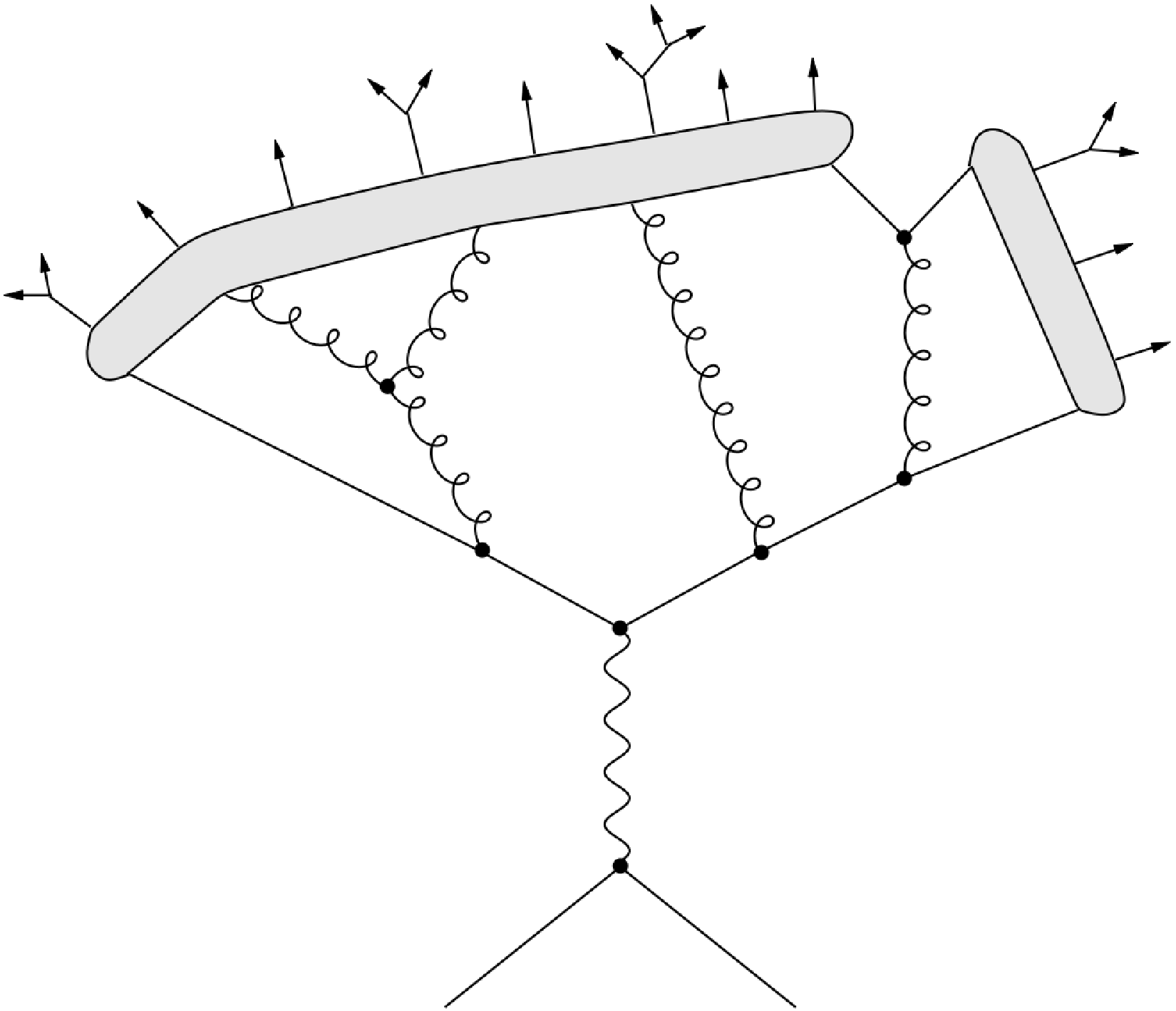

The underlying event In events that contain a hard subprocess, there is extra hadron production that cannot be ascribed to showering from the coloured partons participating in the subprocess, known as the underlying event (UE). Furthermore, this extra activity is greater than that in so-called minimum-bias events (collisions that do not yield an identifiable hard subprocess). The UE is believed to arise from collisions between those partons in the incoming hadrons that do not directly participate in the hard subprocess.
The most common hard subprocess at the LHC is elastic gluon-gluon scattering, . The leading-order differential cross section for this subprocess diverges at zero momentum transfer, due to the exchange of a massless virtual gluon. This divergence is presumably regularized below some momentum transfer, , by higher-order and non-perturbative effects. Nevertheless, for reasonable values of , the integrated cross section for gluon-gluon scattering is very large, larger even than the total proton-proton () scattering cross section. This result indicates that the average number of gluon-gluon collision per collisions is greater than one. Including the cross sections for elastic scattering of quarks, anti-quarks and gluons in all possible combinations (all of which diverge in leading order), multiple parton interactions (MPI) are found to be highly probable
This is the basis on which modern event generators model both minimum-bias collisions and the UE. To account for the extra hadron production when a hard subprocess is present, an event generator must model the impact parameter structure of hadron-hadron collisions. The partons in each incoming hadron are distributed over a transverse area of the order of . The impact parameter of a collision is the transverse distance between the centroids of these areas before the collision. When the impact parameter is large, the areas overlap little and the collision is peripheral; this configuration is associated with a low probability of a hard parton-parton interaction and few MPI. On the other hand, at small impact parameter values, the collision is central and has a large overlap of areas; several multiple interactions and a higher probability of a hard interaction are therefore expected.
To summarize, the presence of a hard subprocess is correlated with more MPI and a higher level of UE activity. Most of the multiple-interactions are soft, though hard MPI is also possible. As mentioned in chapter 1, hard MPI are an important background for e.g., new physics signals involving milti-jet final states. As such, hard MPI are given special attention beyond the general discussion in the context of the UE. The most simple (and often most prominent) case, that of double parton scattering, is reviewed in the next section.
4 Double parton scattering
The formalism to deal with (semi-)hard double parton scattering in hadronic interactions at center-of-mass energy [21, 22] may be summarized by
| (12) | |||||
where is the differential double parton scattering cross section for the inclusive production of a combined system at a given ; the terms denote the differential partonic cross sections for the production of a system in the collision of partons and ; the terms represent double parton distribution functions (DPDFs); and the parameter is a symmetry factor such that if and otherwise. The integration over the momentum fractions and is constrained by energy conservation, such that . Summation over all possible parton combinations is performed. A sketch of double parton scattering is shown in figure 11 for illustration.

The DPDFs, , may be loosely interpreted as the inclusive probability distribution to find a parton with longitudinal momentum fraction at scale in the proton, with the two partons separated by a transverse distance . The scale is given by the characteristic scale of subprocess . It is assumed that the DPDFs may be decomposed into longitudinal and transverse components,
| (13) |
The longitudinal component, , has a rigorous interpretation in leading order pQCD, as the inclusive probability of finding a parton with momentum fraction at scale , as well as and a parton with momentum fraction at scale in a proton. Accurate prediction of double parton scattering cross sections and of event signatures requires good modelling of and of the transverse component, . In particular, one must correctly take account of the effects of correlations in both longitudinal momenta and transverse positions in these functions.
Correlations between the partons in transverse space are highly significant; at the very least, they must tie the two partons together within the same hadron. However, their precise calculation is not possible using perturbation theory. Existing models typically use Gaussian or exponential forms (or their combination) to describe [36, 72]. The transverse component is usually expressed simply as
| (14) |
The quantity is defined at the parton-level, and has the units of a cross section. In the formalism outlined here, it is independent of the process and of the phase-space under consideration. Naively, it may be related to the geometrical size of the proton. That is, given that one hard scattering occurs, the probability of the other hard scattering is proportional to the flux of accompanying partons; these are confined to the colliding protons, and therefore their flux should be inversely proportional to the area (cross section) of a proton. This leads to an estimate of mb, where is the proton radius. Alternatively, may be connected to the inelastic cross section, which would lead to mb at [73, 74]. For hard interactions, assuming uncorrelated scatterings, can be estimated from the gluon form factor of the proton [75] and comes out to be mb.
A number of measurements of have been performed in or collisions at different center-of-mass energies, as specified in table 1.
| Experiment | [GeV] | Final state | [mb] | |
|---|---|---|---|---|
| [23] | AFS (), 1986 | 63 | 4 jets | 5 |
| [24] | UA2 (), 1991 | 630 | 4 jets | 8.3 (95% C.L) |
| [25] | CDF (), 1993 | 1800 | 4 jets | 12.1 |
| [26] | CDF (), 1997 | 1800 | + 3-jets | 14.5 |
| [27] | DØ (), 2010 | 1960 | + 3-jets | 16.4 0.3 2.3 |
| [28] | ATLAS (), 2012 | 7000 | + 2-jets | 15 |
The energy dependence of the measured values of yielded an increase from about 5 mb at the lowest energy () to about 15 mb at LHC energies (). Attempts to explain the differences between these values have used the Constituent Quark Model [76, 77], such as in [78], or have introduced non-trivial correlations between the two scattering systems, as in [16, 17, 18, 19, 20]. A complete explanation, however, is still elusive. A recent argument, suggested in [79, 80, 81] may resolve the discrepancy; it goes as follows. In DPS, two partons from one proton collide with two partons from the other proton. The two partons from a given proton can originate from the non-perturbative hadron wave function or, alternatively, emerge from perturbative splitting of a single parton from the hadron. The former represents a double- interaction, and the latter a interaction. The process could explain the difference between the experimental value of of mb, and the expected value of mb.
In the absence of a rigorous formalism, measurements of typically assume a simple factorization ansatz for the DPDFs,
| (15) |
The differential double parton scattering cross section defined in equation 12 therefore reduces to
| (16) |
The assumption of factorization is problematic. For one, this naive representation does not obey the relevant momentum and number sum rules. In addition, while previous experiments suggest that approximate factorisation holds at moderately low [26], this can not be true for all values of . Namely, if and each satisfy DGLAP evolution, then the naive product, , can not be a solution of the double-DGLAP equations (dDGLAP), suggested e.g., in [17]. In order to use the factorization ansatz, the unknown correlations are absorbed into , which then possibly becomes dependant on the process (and respective phase-space) under consideration.
A measurement of the rate of double parton scattering in four jet events in ATLAS is presented in this thesis, using the simplified form of the effective cross section given in equation 15. Only the double- topology is considered in the analysis, as discussed in chapters 9.
Chapter 3 The ATLAS experiment at the LHC
5 The Large Hadron Collider
The Large Hadron Collider (LHC) is the world’s largest and highest-energy particle accelerator. LHC is a proton-proton () collider, located at the Franco-Swiss border near Geneva, Switzerland. It lies in a tunnel 27 km in circumference at an average depth of 100 meters. The tunnel houses 1232 superconducting bending dipole magnets, cooled using liquid helium to an operating temperature of 1.9 K, producing a magnetic field of about 8 T. The use of dipole magnets allows to keep protons traveling clockwise and counter-clockwise on orbit at the same time. In total, 392 quadrupole magnets are used to keep the beams focused and to collide them at the four interaction points (IPs) of the LHC experiments. The design center-of-mass energy of the LHC is .
Protons are produced by ionizing hydrogen atoms in an electric field. They are injected into RF cavities and accelerated to 750 keV. The beam is then transmitted to the LINAC 2, a linear accelerator, which increases the energy to 50 MeV. The protons are accelerated to 1.4 GeV by the Proton Synchrotron Booster and then further to 26 GeV by the Proton Synchrotron. Next, the Super Proton Synchrotron accelerates the protons to 450 GeV, the minimum energy required to maintain a stable beam in the LHC. Finally, the LHC accelerates them to the operating energy.
During the first two years of operation (2010-2011), the LHC operated at a center-of-mass energy of TeV, with 3.5 TeV per proton. This center-of-mass energy has been chosen to ensure a safe operating margin for the magnets in the accelerator. So far, up to the end of the 2011 run, the LHC delivered 5.61 total integrated luminosity with a peak luminosity of [82]. The bunch separation was 50 ns for most of the running period. The full 2010 and most of the 2011 datasets are used in this analysis.
6 The ATLAS detector
ATLAS (A Toroidal Lhc ApparatuS) [83, 84] is a general-purpose detector surrounding IP 1 of the LHC. ATLAS consists of three main sub-systems, the inner detector (ID), the calorimeters and the muon spectrometer (MS). figure 12a shows a schematic view of the ATLAS detector and its sub-systems.
6.0.1 Detector sub-systems
The ID is used to measure the tracks of charged particles. It covers the pseudo-rapidity range, 22 2 The coordinate system used by ATLAS is a right-handed Cartesian coordinate system. The positive -direction is defined as the direction of the anti-clockwise beam. Pseudo-rapidity is defined as , where is the angle with respect to the -axis. The azimuthal angle in the transverse plane is defined to be zero along the -axis, which points toward the center of the LHC ring., and has full coverage in azimuth. It is made of three main components, arranged in concentric layers, all of which are immersed in a 2 T field provided by the inner solenoid magnet. Three layers of silicon pixel detectors provide a two-dimensional hit position very close to the interaction point. Silicon microstrip detectors are then used in the next four layers, providing excellent position resolution for charged tracks. A transition-radiation detector is the final component of the tracker, with poorer position resolution with respect to the silicon, but providing many measurement points and a large lever-arm for track reconstruction in addition to particle identification capabilities.
The ATLAS calorimeter, shown schematically in figure 12b, is the principal tool used in the analysis.


The calorimeter is composed of several sub-detectors. The liquid argon (LAr) electromagnetic (EM) calorimeter is divided into one barrel () and two end-cap components (). It uses an accordion geometry to ensure fast and uniform response and fine segmentation for optimum reconstruction and identification of electrons and photons. The hadronic scintillator tile calorimeter consists of a barrel covering the region, , and two extended barrels in the range . The LAr hadronic end-cap calorimeter () is located behind the end-cap electromagnetic calorimeter. The forward calorimeter covers the range and also uses LAr as the active material.
The MS forms the outer part of the ATLAS detector and is designed to detect muons exiting the barrel and end-cap calorimeters and to measure their momentum in the pseudo-rapidity range . It is also designed to trigger on muons in the region . The MS operates inside an air-core toroid magnet system with a peak field in the coil windings of 4 T. The precision momentum measurement is performed by the Monitored Drift Tube chambers covering the pseudo-rapidity range (except in the innermost end-cap layer where their coverage is limited to ). In the forward region (), Cathode-Strip Chambers are used in the innermost tracking layer. The capability to trigger on muon tracks is achieved by a system of fast trigger chambers capable of delivering track information within a few tens of nanoseconds after the passage of the particle. In the barrel region (), Resistive Plate Chambers were selected for this purpose, while in the end-cap () Thin Gap Chambers were chosen.
6.0.2 The Trigger System
The ATLAS detector has a three-level trigger system consisting of Level 1 (L1), Level 2 (L2) and Event Filter (EF). The L1 trigger rate at design luminosity is approximately 75 kHz. The L2 and EF triggers reduce the event rate to approximately 200 Hz. Another trigger system used in ATLAS relies on the minimum-bias trigger scintillators (MBTS). The MBTS trigger requires one hit above threshold from either one of the sides of the detector. The different triggers used in the analysis are described in further detail in chapters 6, sections 16.
6.0.3 Luminosity Measurement
Accurate measurement of the delivered luminosity is a key component of the ATLAS physics program. For cross section measurements of SM processes, the uncertainty on the delivered luminosity is often one of the dominant systematic uncertainties.
The instantaneous luminosity of proton-proton collisions can be calculated as
| (17) |
where is the rate of interactions and is the inelastic cross section. Any detector sensitive to inelastic interactions can be used as a source for relative luminosity measurement. However, these detectors must be calibrated using an absolute measurement of the luminosity.
The recorded luminosity can be written as
| (18) |
where is the visible number of interactions per bunch crossing in the detector, is the number of bunch pairs colliding in ATLAS, is the LHC revolution frequency and is the visible cross section, to be determined via calibration for each detector.
The calibration is done using dedicated beam separation scans, also known as van der Meer scans [85], where the two beams are stepped through each other in the horizontal and vertical planes to measure their overlap function. The delivered luminosity is measured using beam parameters,
| (19) |
where and are respectively the bunch populations (protons per bunch) in beam 1 and in beam 2 (together forming the bunch charge product), and and respectively characterize the horizontal and vertical profiles of the colliding beams.
By comparing the delivered luminosity to the peak interaction rate, , observed by a given detector during the van der Meer scan, it is possible to determine the visible cross section,
| (20) |
Two detectors are used to make bunch-by-bunch luminosity measurements in 2010 and in 2011, LUCID and BCM. LUCID is a Cerenkov detector specifically designed for measuring the luminosity in ATLAS. It is made up of sixteen mechanically polished aluminum tubes filled with gas surrounding the beampipe on each side of the IP at a distance of 17 m, covering the pseudo-rapidity range, . The beam conditions monitor (BCM) consists of four small diamond sensors on each side of the ATLAS IP arranged around the beam-pipe in a cross pattern. The BCM is a fast device, primarily designed to monitor background levels. It is also capable of issuing a beam-abort request in cases of possible damage to ATLAS detectors, due to beam losses.
The relative uncertainty on the luminosity scale for collisions during 2010 [86] and 2011 [85] was found to be, respectively 3.4 and 3.9%33 3 The uncertainty on the luminosity in 2011 quoted here is larger than the value given in [85]. The increased value is a consequence of recent studies by the Luminosity group in ATLAS, which show significant non-linear correlations between the van der Meer scans in the horizontal and vertical directions [87]. These correlations were not previously known and are not yet fully understood..
Chapter 4 Monte Carlo simulation
Any analysis involving a complex detector such as ATLAS, requires a detailed detector Monte Carlo (MC) simulation. The MC is used in order to compare distributions of observables, as simulated by physics generators, with the data. In addition, it is used to study the performance of the detector by estimating reconstruction efficiencies, geometrical coverage, the performance of triggers etc.
A description of the MC generators and of the ATLAS detector simulation used in the analysis is presented in the following.
7 Event generators
The four-momenta of particles produced in collisions at the LHC are simulated using various event generators. An overview of MC event generators for LHC physics can be found in [88]. The different MC samples used for comparison with data taken during 2010 and during 2011 are denoted respectively as MC10 and MC11. The following event generators, using different theoretical models, are utilized in the analysis.
Pythia Pythia [89] simulates non-diffractive collisions using a matrix element at leading order in the strong coupling to model the hard subprocess. It uses -ordered parton showers to model additional radiation in the leading-logarithmic approximation [90]. Multiple parton interactions [36, 91], as well as fragmentation and hadronization, based on the Lund string model [69], are also simulated.
Several Pythia 6 tunes utilizing different parton distribution function (PDF) sets are used. The nominal version used in this analysis employs the modified leading-order PDF set, MRST LO* [7]. The parameters used for tuning the underlying event include charged particle spectra measured by ATLAS in minimum bias collisions [92]. The samples used to compare with the 2010 and with the 2011 data respectively use the AMBT1 [93] and AMBT2B [94] tunes.
Several additional combinations of Pythia versions, PDF sets and underlying event tunes are used in chapters 8 in order to evaluate non-perturbative corrections to the dijet mass cross section. These include the following; Pythia 6.425 with the MRST LO* PDF set and the AUET2B [94] tune; Pythia 6.425 with the CTEQ6L1 [8] PDF set and the AMBT2B and AUET2B tunes; Pythia 8 (v150) [95] with the MRST LO** PDF set and 4C [96] tune.
Herwig, Herwig++ Herwig uses a leading order matrix element supplemented with angular-ordered parton showers in the leading-logarithm approximation [97, 98, 99]. The so called cluster model [70] is used for the hadronization. Multiple parton interactions are modelled using Jimmy [100]. The model parameters of Herwig+Jimmy have been tuned to ATLAS data (AUET1 tune) [101]. The MRST LO* PDF set is used.
Herwig++ [102] (v2.5.1) is based on Herwig, but redesigned in the C++ programming language. The generator contains a few modelling improvements. It also uses angular-ordered parton showers, but with an updated evolution variable and a better phase-space treatment. Hadronization is performed using the cluster model, as in Herwig. The underlying event and soft inclusive interactions are described using a hard and soft multiple partonic interactions model [72]. The MRST LO* and the CTEQ6L1 PDF sets are used with the UE7000-3 [94] underlying event tune, in order to evaluate non-perturbative corrections to the dijet mass cross section in chapters 8.
Alpgen Alpgen is a tree level matrix-element generator for hard multi-parton processes () in hadronic collisions [103]. It is interfaced to Herwig to produce parton showers in the leading-logarithmic approximation. Parton showers are matched to the matrix element with the MLM matching scheme [104]. For the hadronization, Herwig is interfaced to Jimmy in order to model soft multiple parton interactions. The PDF set used is CTEQ6L1. Alpgen is used in chapters 8 in order to evaluate the systematic uncertainty associated with the unfolding procedure of the dijet mass cross section measurement.
Sherpa Sherpa is a general-purpose tool for the simulation of particle collisions at high-energy colliders, using a tree-level matrix-element generator for the calculation of hard scattering processes [105]. The emission of additional QCD partons off the initial and final states is described through a parton-shower model. To consistently combine multi-parton matrix elements with the QCD parton cascades, the approach of Catani, Krauss, Kuhn and Webber [106] is employed. A simple model of multiple interactions is used to account for underlying events in hadron–hadron collisions. The fragmentation of partons into primary hadrons is described using a phenomenological cluster-hadronization model [107]. A comprehensive library for simulating tau-lepton and hadron decays is provided. Where available form-factor models and matrix elements are used, allowing for the inclusion of spin correlations; effects of virtual and real QED corrections are included using the approach of Yennie, Frautschi and Suura [108]. The CTEQ6L1 PDF sets together with the default underlying event tune are used. The CKKW matching scale is set at 15 GeV, where the latter refers to the energy scale in which matching of matrix elements to parton showers begins. The implication of this choice is that partons with transverse momentum above 15 GeV in the final state, necessarily originate from matrix elements, and not from the parton shower.
Sherpa is employed in the analysis as part of the double parton scattering measurement in chapters 9. events are generated without multiple interactions, by setting the internal flag, MI_HANDLER=None. The generated events serve as input to a neural network.
8 Simulation of the ATLAS detector
Event samples produced using the different event generators described above are passed through the full ATLAS detector simulation and are reconstructed as the data. The Geant software toolkit [109] within the ATLAS simulation framework [110] propagates the generated particles through the ATLAS detector and simulates their interactions with the detector material. The energy deposited by particles in the active detector material is converted into detector signals with the same format as the ATLAS detector read-out. The simulated detector signals are in turn reconstructed with the same reconstruction software as used for the data.
In Geant the model for the interaction of hadrons with the detector material can be specified for various particle types and for various energy ranges. For the simulation of hadronic interactions in the detector, the Geant set of processes called QGSP_BERT [111] is chosen. In this set of processes, the Quark Gluon String model [112, 113, 114, 115, 116] is used for the fragmentation of the nucleus, and the Bertini cascade model [117, 118, 119, 120] for the description of the interactions of hadrons in the nuclear medium.
The Geant simulation, and in particular the hadronic interaction model for pions and protons, has been validated with test-beam measurements for the barrel [121, 122, 123, 124, 125] and endcap [126, 127, 128] calorimeters. Agreement within a few percent is found between simulation and data for pion momenta between 2 and 350 GeV. Further tests have been carried out in-situ comparing the single hadron response, measured using isolated tracks and identified single particles [129, 130]. Good agreement between simulation and data is found for particle momenta from a few hundred MeV to 6 GeV.
Studies of the material of the inner detector in front of the calorimeters have been performed using secondary hadronic interactions [131]. Additional information is obtained from studying photon conversions [132] and the energy flow in minimum bias events [133]. The ATLAS detector geometry used in the 2010 and in the 2011 simulation campaigns reflects the best current knowledge of the detector at the time the simulations were made. Subsequently, compared to MC10, a more detailed description of the geometry of the LAr calorimeter was used for MC11. The improvement in understanding of the geometry introduced an increased calorimeter response to pions below 10 GeV of about 2%.
The MC11 simulation is made up of different MC-periods. Each MC-period represents different data-taking conditions, such as malfunctioning hardware or changes in the amount of in-time pile-up, additional collisions, coinciding with the hard interaction. Events in the different MC-periods are given relative weights according to the integrated luminosity of the respective data-taking periods they represent.
A note regarding the simulation in chapter 7; before the start of data-taking in 2011, a transitional MC simulation was created, denoted as MC10b. MC10b was generated as part of the MC10 campaign. It used the 2010 simulation settings as described above, with the exception of highly increased pile-up conditions matching the expected characteristics of the 2011 data. The study described in chapter 7 was originally performed using an MC10b Pythia sample. When MC11 became available, most of the results were reproduced; those which were not, are presented here using the previous version of the simulation. Unless otherwise indicated, MC11 is used in conjecture with the 2011 data.
9 Bunch train structure and overlapping events
The LHC bunch train structure of the 2010 and the 2011 data is modelled in MC. In MC10 the simulated collisions are organised in double trains with 225 ns separation. Each train contains eight filled proton bunches with a bunch separation of 150 ns. In MC11 the simulation features four trains with 36 bunches per train and 50 ns spacing between the bunches.
The MC samples are generated with additional minimum bias interactions, using Pythia 6 with the AMBT1 underlying event tune and the MRST LO* PDF set for MC10, and Pythia 6 with the AUET2B tune and the CTEQ6L1 PDF set for MC11. These minimum bias events are used to form pile-up events, which are overlaid onto the hard scattering events. The number of overlaid events follows a Poisson distribution around the average number of additional collisions per bunch crossing, as measured in the experiment. The average number of additional interactions depends on the instantaneous luminosity (see equation 34 in section 17.1); it is thus greater in MC11 compared to MC10, following the trend in the data.
The small separation between bunches in the 2011 data (and respectively in MC11) requires inclusion of the effect of out-of-time pile-up44 4 A feature of the 2011 data is that the signal in the calorimeter is sensitive to collisions from several consecutive bunch crossings; out-of-time pile-up refers to this fact. See section 17 for a detailed discussion. in the simulation. The properties of this effect depend on the distance of the hard scatter events from the beginning of the bunch train. The first ten (approximately) bunch crossings are characterized by increasing out-of-time pile-up contributions from the previous collisions. For the remaining 26 bunch crossings in a train, the out-of-time pile-up is stable within the bunch-to-bunch fluctuations in proton intensity at the LHC.
Chapter 5 Jet reconstruction and calibration
10 Jet reconstruction algorithms
Jets originate from the fragmentation of partons. Due to color flow at the parton-level, there is no one-to-one correspondence between the hadrons inside a jet and the partons which initiated the jet. Because the measurements are performed at the hadron-level and the theoretical expectations at the parton-level, a precise definition of jets is required. The algorithm that relates a jet of hadrons to partons must satisfy,
- -
infrared safety - the presence or absence of additional soft particles between two particles belonging to the same jet should not affect the recombination of these two particles into a jet. Generally, any soft particles not coming from the fragmentation of a hard scattered parton should not affect the number of produced jets;
- -
collinear safety - a jet should be reconstructed independently whether the transverse momentum is carried by one particle, or if that particle is split into two collinear particles;
- -
order independence - the algorithm should be applicable at parton- hadron- or detector-level, and lead to the same origin of the jet.
An illustration of infrared and collinear sensitivity in jet-finding is given in figure 13.


There are many jet algorithms which have been proposed over the years. These include fixed sized cone algorithms as well as sequential recombination algorithms (cluster algorithms), which are based on event shape analysis [134]. The term cone algorithm is applied to a wide range of jet algorithms which broadly aim at maximizing inside a geometric circle in the , coordinates space. The radius of the circle, , is a key parameter of the algorithm. On the other hand, clustering algorithms are based upon pair-wise clustering of the input constituents. In general, an algorithm defines a distance measure between constituents, as well as some condition upon which clustering into a jet should be terminated.
The anti- [135], [136] and Cambridge/Aachen [137, 138] clustering algorithms are used in this analysis. The clustering algorithms begin by computing for each jet constituent, the quantity and for each pair of constituents the quantity , defined as
| (21) | |||||
| (22) |
where
The variables and are constants of the algorithm, and , and are respectively the transverse momentum, the rapidity and the azimuth of the constituent. The parameter, represents the distance between a pair of jet constituents, while is the distance between a given constituent and the beam.
The algorithm proceeds by comparing for each constituent the different values. In the case that the smallest entry is a , constituents and are combined and the list is remade. If the smallest entry is , this constituent is considered a complete jet and is removed from the list.
The variable sets the resolution at which jets are resolved from each other as compared to the beam. For large values of , the are smaller, and thus more merging takes place before jets are complete. The variable can also take different values; for the algorithm , for the Cambridge/Aachen algorithm , and for the anti- algorithm .
The nominal jet collection used for physics in the analysis uses the anti- algorithm with size parameter, , reconstructed with the FastJet package [139]. Jets built with the algorithm are also used, but only as part of the jet energy calibration procedure, as discussed in chapter 7. The Cambridge/Aachen algorithm is used in order to evaluate the systematic uncertainty of said calibration.
11 Inputs to jet reconstruction
11.1 Calorimeter jets
The input to calorimeter jets are topological calorimeter clusters (topo-clusters) [126, 140]. Topo-clusters are groups of calorimeter cells that are designed to follow shower development in the calorimeter. A topo-cluster is defined as having an energy equal to the energy sum of all the included calorimeter cells, zero mass and a reconstructed direction calculated from the weighted averages of the pseudo-rapidities and azimuthal angles of its constituent cells. The weight used in the averaging is the absolute cell energy. The positions of the cells are relative to the nominal ATLAS coordinate system.
Clustering algorithm The topo-cluster algorithm is designed to suppress calorimeter noise. The algorithm starts from a seed cell, whose signal-to-noise () ratio is above a threshold, . Cells neighbouring the seed (or the cluster being formed) that have a signal-to-noise ratio, , are included iteratively. Finally, all calorimeter cells neighbouring the formed topo-cluster are added.
The noise is estimated as the absolute value of the energy deposited in the cell, divided by the RMS of the energy distribution of the cell, measured in events triggered at random bunch crossings. For data taken during 2010, cell-noise was dominated by electronic noise. Due to the shortened bunch crossing interval and increased instantaneous luminosity during 2011 data-taking, the noise increased. An additional component was added, originating from energy deposited in a given cell from previous collisions, but inside the window of sensitivity of the calorimeters. This added energy is referred to as pile-up (see chapter 7 for a detailed discussion). Subsequently, different nominal noise thresholds, , are used to reconstruct topo-clusters in 2010 and in 2011,
| (23) |
Here is the electronic noise, and is the noise from pile-up. On an event-by-event basis, the magnitude of the latter term may vary, as the pile-up is sensitive to the instantaneous luminosity, characterized by the average number of interactions per bunch crossing, , (see section 17.1). A constant baseline is chosen for cluster reconstruction throughout 2011. This baseline corresponds to the noise which results from eight additional pile-up interactions, , and reflects the conditions under which the average effects of pile-up in the 2011 data are minimal.
The change in time of the total nominal noise and its dependence on calorimeter pseudo-rapidity is observed by comparing figures 14a and 14b.


The former shows the energy-equivalent cell-noise in different calorimeter regions in 2010, representing the baseline electronic noise; the latter shows the respective cell-noise in 2011, for which pile-up contributes as well. In most calorimeter regions, the pile-up induced noise is smaller or of the same magnitude as the electronic noise. The exception is the forward calorimeters, where .
The topo-cluster algorithm also includes a splitting step in order to optimise the separation of showers from different close-by particles: All cells in a topo-cluster are searched for local maxima in terms of energy content with a threshold of 500 MeV. This means that the selected calorimeter cell has to be more energetic than any of its neighbours. The local maxima are then used as seeds for a new iteration of topological clustering, which splits the original cluster into more topo-clusters.
Energy scale of clusters Topo-clusters are initially constructed from energy at the electromagnetic (EM) scale. The EM scale correctly reconstructs the energy deposited by particles in an electromagnetic shower in the calorimeter. This energy scale is established using test-beam measurements for electrons in the barrel [142, 143, 144, 145, 121] and the endcap calorimeters [127, 126]. The absolute calorimeter response to energy deposited via electromagnetic processes was validated in the hadronic calorimeters using muons, both from test-beams [121, 146] and produced in-situ by cosmic rays [147]. The energy scale of the electromagnetic calorimeters is corrected using the invariant mass of bosons produced in-situ in proton-proton collisions ( events) [148].
An additional calibration step may also be used, where so called Local Calibration Weights (LCW) are applied to topo-clusters, bringing the clusters to the LCW calibration scale [149]. Starting at the EM scale, topo-clusters are classified as either EM-like or hadron-like, using cluster shape moments. Clusters classified as EM-like are kept at the original energy scale. On the other hand, hadron-like topo-clusters are subject to recalibration. In the first step this entails a cell weighting procedure, which aims to compensate for the lower response of the calorimeter to hadronic deposits. Next, out-of-cluster corrections are applied. These try to account for lost energy deposited in calorimeter cells outside of reconstructed clusters. Finally, dead material corrections are applied, accounting for energy deposits outside of active calorimeter volumes, e.g., in the cryostat, the magnetic coil and calorimeter inter-modular cracks.
Calorimeter jets are built using either EM or LCW scale topo-clusters. In either case, further corrections need to be applied to calibrate jets to the particle-level. This final step is referred to as the jet energy scale (JES) calibration.
11.2 Other types of jets
Track jets Jets can also be built using inner detector tracks as inputs to the jet finding algorithm. Track-based jets, called track jets, are reconstructed using the anti- algorithm with size parameter, . Track jets are required to be composed of at least two tracks; tracks are required to have transverse momentum above 500 MeV, at least one pixel detector hit, at least six hits in the silicon-strip detector, and impact parameters in the transverse plane and in the -direction, both smaller than 1.5 mm. In order to be fully contained in the tracking region, track jets are required to have . Track jets are also required to have transverse momentum larger than 4 GeV.
Truth jets Monte Carlo simulated particle jets are referred to as truth jets. They are defined as those built from stable interacting particles with a lifetime longer than 10 ps in the Monte Carlo event record (excluding muons and neutrinos) that have not been passed through the simulation of the ATLAS detector. Truth jets are built using the anti- algorithm with size parameter , and are required to have transverse momentum larger than 10 GeV.
12 Jet energy calibration
The jet energy calibration relates the jet energy measured with the ATLAS calorimeter to the true energy of the corresponding jet of stable particles entering the detector. The jet calibration corrects for the following detector effects that affect the jet energy measurement;
- -
calorimeter non-compensation - partial measurement of the energy deposited by hadrons;
- -
dead material - energy losses in inactive regions of the detector;
- -
leakage - energy of particles reaching outside the calorimeters;
- -
out of calorimeter jet cone - energy deposits of particles which are not included in the reconstructed jet, but were part of the corresponding truth jet and entered the detector;
- -
noise thresholds and particle reconstruction efficiency - signal losses in calorimeter clustering and jet reconstruction.
Jets reconstructed in the calorimeter system are formed from calorimeter energy depositions reconstructed at either the EM or the LCW scale, as described above. The correction for the lower response to hadrons is solely based on the topology of the energy depositions observed in the calorimeter. The measured jet energy is corrected on average, using:
| (24) |
Here is the calorimeter energy measured at the EM or LCW scales, denoted collectively by S. The variable is the hadron-level calibrated jet energy, and is a calibration function. The latter depends on the measured jet energy, and is evaluated in small jet-pseudo-rapidity, , regions. The baseline Pythia MC samples described in chapter 4 are used to derive ; the procedure is explained in the following.
The variable denotes the EM- or LCW-level energy after the contribution of pile-up (additional multiple proton-proton interactions) has been subtracted. The pile-up energy is expressed through the function , called the jet offset correction. The offset correction in 2010 and in 2011 depends on the number of collisions which occur within the same bunch crossing as the collision of interest. This is referred to as in-time pile-up and is estimated by the number of primary vertices, , in a given event. In addition, exhibits a strong rapidity dependence, due to the varying calorimeter response in , and to the rapidity distribution of the pile-up interactions. The offset correction is parametrized separately for EM and for LCW jets, based in each case on jet constituents which are calibrated in the respective energy scale.
The offset correction performs well for data taken in 2010 [150]. For the case of the 2011 data, the nature of pile-up becomes more complicated, as interactions in bunch crossings proceeding and following the event of interest affect the signal in the calorimeter; this effect is called out-of-time pile-up. The offset correction is modified in 2011 in order to account for this effect, but the performance is nonetheless degraded with regard to 2010. A detailed discussion of out-of-time pile-up and the exact functional form of are given in section 17. An alternative to the offset correction using a data-driven method, referred to as the jet area/median method, is introduced in chapter 7. The offset correction is used for the calibration of jets in the 2010 data in this analysis; the jet median approach is used as the nominal pile-up correction for the 2011 data.
The two calibrations schemes, which respectively use jets constructed from either EM- or LCW-calibrated topo-clusters, are referred to as EM+JES and LCW+JES. For data taken during 2010, only the simpler EM+JES calibration is available for this analysis. For the 2011 data, the nominal jet collection is calibrated using LCW+JES. The calibration schemes include several steps, described in the following:
- -
jet origin correction;
- -
jet energy correction;
- -
jet pseudo-rapidity correction;
- -
residual in-situ calibration (2011 data only).
Jet origin correction Calorimeter jets are reconstructed using the geometrical center of the ATLAS detector as reference to calculate the direction of jets and their constituents. The jet four-momentum is corrected for each event such that the direction of each topo-cluster points back to the primary (highest-) reconstructed vertex. The kinematic observables of each topo-cluster are recalculated using the vector from the primary vertex to the topo-cluster centroid as its direction. The raw jet four-momentum is thereafter redefined as the vector sum of the topo-cluster four-momenta. This correction improves the angular resolution and results in a small improvement () in the jet response. The jet energy is unaffected.
Jet energy correction The principle step of the EM+JES and of the LCW+JES jet calibrations restores the reconstructed jet energy to the energy of the corresponding MC truth jet. Since pile-up effects have already been accounted for, the MC samples used to derive the calibration do not include multiple interactions.
The calibration is derived using isolated calorimeter jets that have a matching isolated truth jet within . Distance is defined in , space as
| (25) |
where () and () are respectively the azimuthal angles (pseudo-rapidities) of truth and reconstructed jets. An isolated jet is defined as one having no other jet with within , where is the size parameter of the jet algorithm.
The final jet energy scale calibration is parametrised as a function of detector-level pseudo-rapidity, ,55 5 Here, pseudo-rapidity refers to that of the original reconstructed jet before the origin correction. and of jet energy at the detector-level energy scales, . In the following, as above, S stands for either the EM or the LCW energy scales. The detector-level jet energy-response,
| (26) |
is measured for each pair of calorimeter and truth jets in bins of truth jet energy, , and of . For each -bin, the averaged jet-response, , is defined as the peak position of a Gaussian fit to the distribution. In addition, in the same -bin, the average jet energy-response, , is derived from the mean of the distribution of .
For a given -bin, , the jet energy-response calibration function, , is obtained using a fit of the values for each -bin . The fitting function is parameterised as
| (27) |
where are free parameters, and is chosen between and , depending on the goodness of the fit.
The final jet energy scale correction that relates the measured calorimeter jet energy to the true energy, is then defined as in the following:
| (28) |
where is the jet-response calibration function for the relevant -bin .
As an example, the average jet energy scale correction for EM jets in 2010, , is shown as a function of calibrated jet for three -intervals in figure 15a. The response of 2010 EM+JES jets, , is shown for various energy and -bins in figure 15b.


Average simulated jet-response at the EM scale in bins of detector pseudo-rapidity, . Different jet energies, , are represented (using EM+JES jets) as indicated in the figure. The parallel lines mark the regions over which the JES correction is evaluated. The inverse of the response shown in each bin is equal to the average jet energy scale correction.
(Figures are taken from [150].)
As the transverse momentum of jets increases, the response and subsequent JES correction factor decrease. The corrections is also highly rapidity-dependant, due in part to the changing structure of calorimeter elements; in transition regions of the calorimeter (around ) the response is significantly higher, due to energy loss in dead material or through leakage. Larger correction factors are therefore required in these regions. Corresponding figures for 2011 LCW+JES jets may be found in [151].
Jet pseudo-rapidity correction After the jet origin and energy corrections, the origin-corrected pseudo-rapidity of jets is further corrected for a bias due to poorly instrumented regions of the calorimeter. In these regions topo-clusters are reconstructed with a lower energy with respect to better instrumented regions (see figure 15b). This causes the jet direction to be biased towards the better instrumented calorimeter regions.
The -correction is derived as the average difference between the pseudo-rapidity of reconstructed jets and their truth jet counterparts. It is parametrized according to the energy and detector-level pseudo-rapidity of reconstructed jets, . The correction is very small for most regions of the calorimeter, and up to five times larger in the transition regions.
Residual in-situ calibration (2011 data only) Following the pseudo-rapidity correction, the transverse momentum of jets in the 2011 data is compared to that in MC using in-situ techniques. The latter exploit the balance between the transverse momentum of a jet, , and that of a reference object, [151]. The ratio,
| (29) |
called the residual in-situ JES correction, is used on jets measured in data. It is derived using the following methods:
- -
the of jets within is equalized to the of jets within , exploiting the balance between central and forward jets in events with only two high jets;
- -
an in-situ JES correction for jets within is derived using the of a photon or a boson (decaying to or ) as reference;
- -
events where a system of low- jets recoils against a high- jet are used to calibrate jets in the TeV regime. The low- and high- jets are required to respectively be within and .
13 Jet quality selection
Jets at high transverse momenta produced in collisions must be distinguished from background jets not originating from hard scattering events. The main sources of background are listed in the following:
- -
large calorimeter noise;
- -
beam-gas events, where one proton of the beam collided with the residual gas within the beam pipe;
- -
beam-halo events, e.g., caused by interactions in the tertiary collimators in the beam-line far away from the ATLAS detector;
- -
cosmic ray muons overlapping in-time with collision events.
These backgrounds are divided into two categories, calorimeter noise and non-collision interactions.
Calorimeter noise - two types of calorimeter noise are addressed, sporadic noise bursts and coherent noise. Sporadic noise bursts in the hadronic endcap calorimeter (HEC) commonly result in a single noisy calorimeter cell, which contributes almost all of the energy of a jet. Such jets are therefore rejected if they have high HEC energy fractions, denoted by . The signal shape quality, , may also be used for rejection, the latter being a measure of the pulse shape of a calorimeter cell compared to nominal conditions. Due to the capacitive coupling between channels, neighbouring calorimeter cells around the noise burst have an apparent negative energy, denoted by . A hight value of is therefore used to distinguish jets which originate in noise bursts. On rare occasions, coherent noise in the electromagnetic calorimeter develops. Fake jets arising from this background are characterised by a large EM energy fraction, , which is the ratio of the energy deposited in the EM calorimeter to the total energy. Similar to the case of noise bursts in the HEC, a large fraction of calorimeter cells exhibit poor signal shape quality, , in such cases.
Non-collision backgrounds - cosmic rays or non-collision interactions are likely to induce events where jet candidates are not in-time with the beam collision. A cut on the jet-time, , may therefore be applied to reject such jets. Jet-time is reconstructed from the energy deposition in the calorimeter by weighting the reconstructed time of calorimeter cells forming the jet with the square of the cell energy. The calorimeter time is defined with respect to the event time (recorded by the trigger). A cut on is applied to make sure that jets have some energy deposited in the calorimeter layer closest to the interaction region, as expected for a jet originating from the nominal interaction point. Since real jets are expected to have tracks, the cut may be applied together with a cut on the jet charged fraction, , defined as the ratio of the scalar sum of the of the tracks associated to the jet, divided by the jet . The jet charged fraction cut is, naturally, only applicable for jets within the acceptance of the tracker. A cut on the maximum energy fraction in any single calorimeter layer, , is applied to further reject non-collision background.
Two sets of quality criteria are defined, denoted as Loose and Medium selection. These incorporate requirements on the rejection variables defined above, and are specified in detail in appendix 11.A, appendix 11.A. For the 2010 data, the tighter, Medium selection, is required. Since these criteria are not fully efficient, an efficiency correction is applied to jets. The selection efficiency for jets in two pseudo-rapidity regions is shown in figure 16 for illustration.


In general, for transverse momenta larger than , the efficiency is above 99% across all rapidities. For lower jet , efficiencies range between 96-98% within , and are above 99% otherwise. Further details are available in [150]. For the 2011 data, due to improved understanding of the calorimeter, a reduced version of the 2010 Loose selection is used. The efficiency is above 99.8% for jets with GeV across all rapidities.
14 Systematic uncertainties on the kinematic properties of jets
14.1 Jet energy scale uncertainties
The systematic uncertainty associated with the jet energy scale (JES) is the primary source of uncertainty in the analysis. It has been determined for the 2010 and 2011 datasets in [152] and in [151], using integrated luminosities of and , respectively. In total seven sources of uncertainty on the jet energy scale are considered in 2010 and thirteen in 2011.
The sources of uncertainty on the 2010 measurement are the following:
- -
single hadron response - uncertainty associated with the response of a single particle entering the calorimeter. Discrepancies may arise due to the limited knowledge of the exact detector geometry; due to the presence of additional dead material; and due to the modelling of the exact way particles interact in the detector;
- -
cluster thresholds - uncertainty associated with the thresholds for reconstructing topo-clusters. The clustering algorithm is based on the signal-to-noise ratio of calorimeter cells. Discrepancies between the simulated noise and the real noise, or changes in time of the noise in data, can lead to differences in the cluster shapes and to the presence of fake topo-clusters;
- -
Perugia 2010 and Alpgen+Herwig+Jimmy - uncertainty associated with the modelling of fragmentation and the underlying event, or with other choices in the event modelling of the MC generator. The response predicted by the nominal Pythia generator are compared to the Pythia Perugia 2010 tune and to Alpgen, coupled to Herwig and Jimmy;
- -
intercalibration - uncertainty associated with the rapidity-intercalibration method, in which dijet events are used in-situ to measure the response in two regions in the calorimeter. The measurement is done in different rapidity intervals simultaneously, by minimizing a response matrix. The uncertainty is estimated by comparing the response with that measured in-situ in events in which one of the jets is constrained to be central;
- -
relative non-closure - uncertainty associated with the non-closure of the energy of jets in MC following the JES calibration;
- -
in-time pile-up - uncertainty associated with the simulation and subtraction of in-time pile-up.
For the LCW+JES calibration scheme, which is used in this analysis for the 2011 dataset, the baseline JES uncertainty is estimated using a combination of in-situ techniques. In total, the different sources of uncertainty coming from the in-situ techniques in 2011 data amount to 60 components. These are combined, assuming they are fully correlated in and , into six effective nuisance parameters (ENP). The combination procedure involves diagonalizing the covariance matrix of the JES correction factors and selecting the five eigenvectors that have the largest corresponding eigenvalues. An additional sixth effective parameter represents all residual sources of uncertainty.
The sources of uncertainty on the 2011 measurement are the following:
- -
ENP 1-6 - uncertainty associated with the six effective nuisance parameters, which combine the 60 components of the in-situ methods used to estimate the JES uncertainty in 2011;
- -
intercalibration, single hadron response and relative non-closure - same as for 2010;
- -
close-by jets - uncertainty associated with event topologies in which two jets are reconstructed in close proximity;
- -
in-time PU, out-of-time PU and PU pt - uncertainty associated with the simulation and subtraction of in- and out-of-time pile-up.
The final fractional JES uncertainties for the 2010 and the 2011 data are compared in figure 17 as a function of the of jets in the central region.


The uncertainty on the 2011 data is much improved compared to 2010. This is due both to the increase in 2011 in the statistics which are used to derive uncertainty, and to the use of sophisticated in-situ techniques. For EM+JES jet in 2010 the total uncertainty is roughly 2% for jets with GeV, increasing up to roughly twice that for lower or higher transverse momenta. For LCW+JES jets in 2011, the uncertainty is roughly 1% in the respective mid- range, increasing up to 2% between 20 and 40 GeV and up to 4% between 0.5 and 2 TeV.
14.2 Jet energy and angular resolution
In addition to the jet energy scale, which is the primary source of uncertainty for most measurements involving jets, the jet energy and angular resolution must also be taken into account. These are addressed in the following.
Jet energy resolution The baseline parameterization of the jet energy resolution in MC is derived using the nominal Pythia MC simulation for jets with transverse momentum, GeV [153]. In-situ measurements are also made for jets with rapidities, and GeV. In this kinematic range, the comparison of the resolution measured with the in-situ techniques between the data and the MC shows agreement better than 10%. The uncertainty on the jet energy resolution for each rapidity region is assigned from the weighted average of the systematic errors on the relative difference between the data and the MC, and is flat as a function of . Outside the kinematic range of in-situ measurements, the MC parameterization is kept but the uncertainty is conservatively increased.
In order to illustrate the behaviour of the transverse momentum resolution in MC, the relative transverse momentum offset between the of a truth jet, , and that of the corresponding matched reconstructed jet, , is defined as
| (30) |
Matching is performed by selecting a reconstructed jet within distance of the truth jet, where is the size parameter of the jet. In order to keep the sample pure, isolation of the matched truth jets from their counterparts within is also imposed.
The average relative transverse momentum offset represents the fractional bias in of jets. The relative resolution is parametrized by the width of the distribution of , denoted by . The dependence of the average and of on truth jet is shown in figure 18 for jets in different pseudo-rapidity regions in MC10 and in MC11.


At GeV in 2010 and at GeV in 2011, changes sign. These transverse momentum values mark the corresponding thresholds in either year for which the energy calibration of jets becomes valid. The relative bias in transverse momentum is lower in absolute value than 1% (6%) for jets with GeV within () in 2010. In 2011, the bias is lower than 2% for central jets within . For higher values of transverse momentum the relative bias decreases, becoming negligible for non-central jets in 2010 above 200 GeV and for central jets in 2011 above 100 GeV. The relative resolution, , is also rapidity- and momentum-dependent. For the various -regions the relative resolution decreases from 21% in 2010 (and 27% in 2011) for jets with , down to 4-6% for jets with GeV. Both and are generally higher for low- jets in MC11 compared to MC10, due to the increase in pile-up in 2011.
Jet angular resolution In addition to the resolution, the rapidity and azimuthal resolutions are used in section 26 to estimated a component of the systematic uncertainty associated with the dijet mass measurement. A parametrization of the angular resolutions for different jet transverse momenta and rapidities is derived from the following.
The pseudo-rapidity offset and the azimuthal offset of jets are respectively defined in MC as
| (31) |
by matching truth and reconstructed jets, as discussed with regard to equation 30. Here, as before, () and () are respectively the pseudo-rapidities (azimuthal angles) of truth and reconstructed jets. The parameters and represents the angular bias of jets. The width of the distributions of and represent the angular resolution of jets, denoted respectively as and .
The dependence of the average angular offset parameters and of the angular resolution parameters on truth jet is shown in figures 19 - 20 for jets in different pseudo-rapidity regions in MC10 and in MC11.


The pseudo-rapidity offset is smaller than in all regions for jets with low in 2010, becoming insignificant for transverse momentum values above . For jets in 2011 a small bias of roughly is observed for all regions. The resolution is roughly 0.04 for jets with in MC10 and for jets with in MC11. For jets with higher transverse momenta, the resolution decreases, reaching values smaller than above . The slightly degraded performance for jets in 2011 compared to 2010 is due the increase in pile-up.
The azimuthal offset and resolution follow similar trends as do the pseudo-rapidity offset and resolution parameters. The magnitude of the offset is smaller than for low jets, becoming insignificant (consistent with zero within errors) above . The azimuthal resolution also improves with growing jet , decreasing from 0.07 for jets with () to roughly 0.02 above for jets in MC10 (MC11).
Chapter 6 Data selection
15 Dataset
The measurements presented in this thesis are performed on data of collisions at , collected by the ATLAS experiment during 2010 and during 2011. The former include all data taken during 2010 with two exceptions, for the low- and the forward regions. For the low- region (events where the highest- jet has GeV), only data runs taken up to the beginning of June are considered. For these data the instantaneous luminosity of the accelerator was low enough that pile-up contributions were negligible, and the majority of the bandwidth was allocated to the minimum bias trigger. The forward jet trigger (covering rapidities ) was not active in the first data-taking period.
The 2011 dataset includes data taken during April, and between July and October, corresponding respectively to 2011 periods D and I–M. Before period D, the LHC was not operating at the nominal data-taking conditions used in this analysis; the solenoid and/or toroid fields were off, the bunch train frequency was varied and the center-of-mass energy was changed. Data taken during these periods are therefore not included in this analysis. In data periods E–H, corresponding to 20% of the luminosity recorded in 2011, six LAr Front End Boards (FEBs) were lost. LAr FEBs contain the electronics for amplifying, shaping, sampling, pipelining, and digitizing the liquid argon calorimeter signals. As a result, a region, in pseudo-rapidity and in azimuth were affected. Jets which fell in this area of the calorimeter suffered a 30% loss in energy and a increase in energy resolution at high . Data periods E–H are therefore excluded from the analysis.
All data events considered in the following require good detector status for the L1 central trigger processor, solenoid magnet, inner detectors (Pixel, SCT, and TRT), calorimeters (barrel, endcap, and forward), luminosity, as well as tracking, jet, and missing energy reconstruction performance. In addition, good data quality is required for the high-level trigger during the periods when this device is used for rejection. Events have at least one reconstructed vertex; vertices are reconstructed with constraints on their associated ID tracks, and are consistent with the beam-spot.
In total of data taken during 2010, and of data taken during 2011, are used in the analysis.
16 Trigger and luminosity
16.1 Description of the trigger
Four different triggers are used in this analysis, a random trigger, the central jet trigger (), the forward jet trigger (), and the minimum bias trigger (MBTS).
The central and forward jet triggers are composed of three consecutive levels; Level 1 (L1), Level 2 (L2) and Event Filter (EF). The central and forward jet triggers independently select data using several jet transverse energy thresholds that each require the presence of a jet with sufficient transverse energy at the electromagnetic (EM) scale, . For each L1 threshold, there is a corresponding L2 threshold that is generally placed 15 GeV above the L1 value. The following convention is used for jet trigger names; names begin with the trigger-level and end with a number. The number stands for the trigger threshold, such that e.g., L1_J5 is a Level 1 trigger with a threshold, GeV. Jet trigger names also contain a “regional” identifier, the letter J for central triggers, and the combination FJ for forward triggers.
The MBTS trigger (denoted by L1_MBTS at Level 1 and by EF_MBTS for the Event Filter) requires at least one hit in the minimum bias scintillators located in front of the endcap cryostats, covering , and is the primary trigger used to select minimum-bias events in ATLAS. It has been demonstrated to have negligible inefficiency for the events of interest for this analysis [154] and is generally used to select events with low- jets. It is used in this study only for data taken during 2010. Events with low- jets in 2011 data are selected using a random trigger.
The complete list of triggers used in the analysis in the different data-taking periods is given in table 7 - 9 in appendix 11.B.
16.2 Trigger efficiency
The per-jet efficiency is determined from the probability that a single jet passes a given trigger threshold, regardless of what the other jets in the event do. In order to determine the efficiency, the off-line reconstructed jets are matched to central or forward trigger objects by the shortest distance,
using the pseudo-rapidity and azimuth of the trigger object, and , and of the selected jet, and .
There is an ambiguity whether to associate a jet in the transition region to a central or to a forward trigger object. The rapidity resolution between off-line jets and L1 trigger objects, which seed the higher trigger chain, can therefore lead to central trigger objects that are reconstructed as forward jets, and vice versa. The problem is aggravated by the fact that the forward L1 jet trigger has no information in the FCal. In order to resolve the ambiguity, two candidate trigger objects are assigned to an off-line jet, one from the central and one from the forward trigger systems. This is done using all available information, that is, central trigger objects are matched by the smallest with respect to the selected jet, and forward trigger objects by the smallest . In the next step, the candidate which is closest to the off-line jet between the two is chosen. A detailed description of the matching procedure may be found in [155].
The efficiencies for various central jet triggers are shown in figure 21 for the 2010 and for the 2011 data.


Additional rapidity bins are presented in appendix 11.B, appendix 11.B - 74. These include three regions: The first is the crack region between the calorimeter barrel and endcap, ; there, the per-jet L1 and L2 trigger efficiencies never become fully efficient due to calorimeter inhomogeneities. The second is the transition region between the central and the forward trigger systems, ; in this region, trigger selection is performed by matching jets to either the central or the forward triggers, as described above. The third is the forward region, , where the forward jet trigger is used; due to a dead FCal trigger tower that spans a width of in the rapidity region , the forward jet triggers are not fully efficient in this region.
As the instantaneous luminosity increased throughout data-taking, it was necessary to prescale triggers with lower thresholds. For each bin of jet- considered in this analysis, a dedicated trigger threshold is chosen such that the efficiency is as close as possible to 100% and the prescale is as small as possible. table 2 presents the various triggers used in the analysis as a function of jet transverse momenta and rapidity, for data taken throughout 2010. The per-jet trigger efficiencies are shown in appendix 11.B, table 6.
| [ GeV ] | Trigger name | |||||
|---|---|---|---|---|---|---|
| Period A | Periods A-D | Periods E-F | Periods G-I | |||
| Run 152777 | (Run 152777) | (excl. E1-E4) | ||||
| 20 | 42.5 | L1_MBTS | L1_MBTS | L1_MBTS | EF_MBTS | |
| 42.5 | 70 | L1_MBTS | L1_J5 | L1_J5 | L2_J15 | |
| 70 | 97.5 | L1_MBTS | L1_J15 | L1_J15 | L2_J30 | |
| 97.5 | 152.5 | L1_MBTS | L1_J30 | L1_J30 | L2_J45 | |
| 152.5 | 197.5 | L1_MBTS | L1_J55 | L1_J55 | L2_J70 | |
| 197.5 | 217.5 | L1_MBTS | L1_J55 | L1_J55 | L2_J90 | |
| 217.5 | L1_MBTS | L1_J55 | L1_J55 | L1_j95 | ||
| 20 | 42.5 | L1_MBTS | L1_MBTS | L1_MBTS | EF_MBTS | |
| 42.5 | 62.5 | L1_MBTS | L1_MBTS | L1_FJ10 | EF_MBTS | |
| 62.5 | 72.5 | L1_MBTS | L1_MBTS | L1_FJ10 | L2_FJ25 | |
| 72.5 | 95 | L1_MBTS | L1_MBTS | L1_FJ30 | L2_FJ25 | |
| 95 | 160 | L1_MBTS | L1_MBTS | L1_FJ30 | L2_FJ45 | |
| 160 | L1_MBTS | L1_MBTS | L1_FJ30 | L2_FJ70 | ||
| 20 | 42.5 | L1_MBTS | L1_MBTS | L1_FJ10 | EF_MBTS | |
| 42.5 | 50 | L1_MBTS | L1_MBTS | L1_FJ10 | L2_FJ25 | |
| 50 | 67.5 | L1_MBTS | L1_MBTS | L1_FJ30 | L2_FJ25 | |
| 67.5 | 100 | L1_MBTS | L1_MBTS | L1_FJ30 | L2_FJ45 | |
| 100 | L1_MBTS | L1_MBTS | L1_FJ30 | L2_FJ70 | ||
| [ GeV ] | Trigger name | ||
|---|---|---|---|
| Periods D,I-M | |||
| 20 | 47 | EF_rd0 | |
| 47 | 52 | EF_J10 | |
| 52 | 60 | EF_J15 | |
| 60 | 82 | EF_J20 | |
| 82 | 97 | EF_J30 | |
| 97 | 122 | EF_J40 | |
| 122 | 160 | EF_J55 | |
| 160 | 207 | EF_J75 | |
| 207 | 275 | EF_J100 | |
| 275 | 365 | EF_J135 | |
| 365 | 472 | EF_J180 | |
| 472 | EF_J240 | ||
The triggers used for the 2011 data are listed in table 3. The EF triggers used in 2011 have efficiency within the rapidity region of interest ().
16.3 Luminosity calculation using a two-trigger selection scheme
A two-trigger strategy is used in the analysis, following the prescription employed in [156]. An event may be accepted if at least one of the two leading (highest-) jets passes a dedicated trigger, determined by the transverse momentum and pseudo-rapidity of the jet. The event is then assigned to one of two luminosity classes, or . The former, a single-trigger luminosity class, is for events where the two jets are assigned to the same trigger. The latter, a double-trigger luminosity class, is for events in which each jet is assigned to a different trigger.
In order to account for different prescale combinations of the two jets, the Inclusive method for fully efficient combinations [157] is used. This method entails calculation of the integrated luminosity of each trigger over the entire event sample, and combination of the per-trigger luminosities on an event-by-event basis. Let denote the integrated luminosity in a luminosity-block (LB), and let denote the prescale of a given jet trigger within this LB. The effective luminosity of a single trigger for the entire dataset can then be written as
| (32) |
where the summation is over all luminosity-blocks. The effective luminosity for a pair of triggers takes into account the probability that two triggers with prescales, and , fired simultaneously in a given event; it is defined by
| (33) |
table 7 - 9 in appendix 11.B show the integrated single- and double-trigger luminosities for the different trigger-bins used in the analysis.
The combined trigger efficiency of the two leading jets is computed in a similar manner as in equation 33, using the corresponding per-jet trigger efficiencies (given in table 6 for the 2010 data and taken as unity for the 2011 data) and the single-jet reconstruction efficiency (see section 13). Together these yield the probability for an event to have fired a given trigger (or trigger combination), and for a jet (or pair of jets) to have been reconstructed and matched to the trigger(s). The inverse of the combined trigger and reconstruction efficiency factor is multiplied by the luminosity of the selected luminosity class; this produces the final luminosity weight for each event.
Chapter 7 The jet area/median method for pile-up subtraction
As discussed in sections 12, an important component of the energy calibration of jets is the subtraction of pile-up, that is the extra energy which originates from additional interactions that occurred in the same bunch-crossing. The current strategy in ATLAS for dealing with pile-up involves the subtraction of an average correction derived from MC simulation, called the offset correction. The offset correction is parametrized in variables which reflect the magnitude of the different components of the pile-up in a given event. As the parametrization is derived from MC, it suffers from uncertainties due to miss-modelling of the pile-up and requires adjustments based on in-situ measurements.
In the following, an alternative data-driven method is introduced, called the jet area/median method. The median method combines parametrization of the average contributions of pile-up in data, as well as an event-by-event estimation of the local pile-up energy around the jets of interest. The median correction is used to calibrate the energy of jets in data taken during 2011, and the performance is compared to the default offset correction.
As mentioned in section 8, a few of the results shown in the following use the transitional simulation, MC10b. Unless otherwise indicated, MC11 is used.
17 Pile-up in ATLAS
17.1 In- and out-of-time pile-up
Pile-up in ATLAS is usually separated into in-time pile-up and out-of-time pile-up. The former refers to the number of collisions which occur within the same bunch crossing as the collision of interest, and the latter to interactions in previous or subsequent bunch crossings. The exact nature of out-of-time pile-up depends on the bunch-structure of the LHC, and on the specifics of the reconstruction of calorimeter signals.
For the data used in this study, the spacing between adjacent bunches was 50 ns. This number should be compared with the typical signal shaping time of the liquid Argon calorimeters, which is roughly 400 ns [158], as illustrated in figure 22.

The figure shows the shaped signal in a typical calorimeter element (cell). The shaping integrates the electronic signal registered in the cell in two phases. In the first phase, which takes , the signal is integrated with a positive amplitude. In the second phase, which takes , the signal is integrated with a negative amplitude; the latter is smaller in magnitude compared to the positive amplitude in the first phase. The shaping is such that the total integral of the positive- and the negative-amplitude phases is zero, such that for the case of random noise, the integrated signal is minimal.
A consequence of the long integration time (compared to the short bunch crossing rate) is that the energy deposits from several bunch crossings are typically overlaid with any event of interest. The situation is further complicated by the mixture of positive and negative amplitudes of the shaping. The resulting pile-up signal can therefore be composed of both positive- and negative-energy components within a given 50 ns readout window. The shaping is designed such that out-of-time pile-up should have an overall negative effect that cancels the positive effect from in-time pile-up on average. However, this only works if the bunch intensity and subsequent occupancy of cells is constant over the integration time of the calorimeter. By design of the shaping amplifier, the most efficient suppression is achieved for 25 ns bunch spacing in the LHC beams. The 2011 beam conditions, with 50 ns bunch spacing, do not allow for full pile-up suppression by signal shaping. In addition, a given cell would not necessarily have contributions from pile-up from every bunch crossing, and so while there is approximate cancellation of positive and negative pile-up on average, there are large fluctuations on an even-by-event basis. Special attention must also be given to the position of the bunch crossing within the bunch train. For example, at the beginning of a bunch train there is insufficient out-of-time pile-up to cancel the in-time pile-up; the calorimeter response in such events is therefore systematically higher.
During reconstruction, calorimeter cells are combined into topo-clusters (see section 11). Due to the presence of the negative-energy signals, two effects come into play; the positive energy of positive topo-clusters is reduced, and purely negative-energy topo-clusters are formed. In the current jet reconstruction scheme of ATLAS, there is no calibration for negative-energy jet constituents, therefore these are discarded and not used in the reconstructing of jets. The energy of a jet which includes positive- and negative-energy cells is subsequently not a simple linear combination of cell energies. Rather, it is the sum of energies of those positive-energy clusters, which had enough positive-energy cells to pass the reconstruction threshold.
For the 2010 data, the relatively large spacing between adjacent bunches and the low instantaneous luminosity mean that the magnitude of the out-of-time pile-up is negligible. Consequently, out-of-time pile-up is only discussed here in the context of the 2011 data and MC.
On average, one can parametrize the amount of energy originating from pile-up by the number of interactions, which is measured by counting the number of reconstructed vertices in a given event, .
Vertices are reconstructed from ID tracks, with a requirement of at least five or three tracks per vertex for data taken respectively during 2010 or 2011. Tracks are selected in 2010 and in 2011 using the following criteria:
| 2010: | ||
|---|---|---|
| 2011: | ||
Here is the transverse momentum of a track and and are respectively the number of hits from the pixel and SCT detectors that are associated with the track. The parameters and are the transverse and longitudinal impact parameters measured with respect to the vertex to which the tracks are extrapolated. The ratio represents the quality of the fit of the track parameters divided by the number of degrees of freedom of the fit. Vertices are also required to be consistent with the beam-spot.
The constraints on vertex reconstruction used here for the 2011 data are tighter than what is usually used in analyses in ATLAS, in that the common 2011 selection criteria do not impose the track selection requirements described above. Vertices selected with these looser constraints will be referred to as in the following. The relation between the average of and is shown in figure 23a for reference. The relation between the two definitions is linear, suggesting that on average the two factors provide equivalent characterization of the amount of in-time pile-up in an event. The MC describes the data well.
The number of in-time interactions, , contributes purely-positive pile-up energy to a given event. Depending on the position of a given collision within the bunch train, out-of-time pile-up has on average different negative and positive energy components. In order to estimate the amount of out-of-time pile-up, one would in principle need to measure during collisions before and after the event of interest, within a time window of ns. Due to the trigger strategy of ATLAS, these events may have been discarded. Subsequently, the only handle on out-of-time pile-up is the average number of collisions in a given time-frame, which depends on the instantaneous luminosity. The number of collisions is described by a Poissonian distribution with some mean value, . The mean is computed over a rather large window in time, , which safely encompasses the time interval during which the ATLAS calorimeter signal is sensitive to the activity in the collision history ( ns for the liquid argon calorimeters). The average number of interactions can be reconstructed from the average luminosity over this time window, , the total inelastic cross section, mb [159], the number of colliding bunches in LHC, , and the LHC revolution frequency, , [86]
| (34) |
The correlation between and the average is shown in figure 23b for data taken during 2011 and for the nominal MC11 Pythia simulation.


The average, , as a function of the average number of interactions, .
As indicated in the figures, data taken during 2011 are compared to MC11 in the top panels, and the ratio of data to MC is shown in the bottom panels.
There is strong correlation between the two factors, as expected. Good agreement is observed between the data and the MC.
In order to properly describe pile-up in data, MC samples are weighted such that the distributions of the number of reconstructed vertices in MC10 and MC11 match the respective distributions in the 2010 and in the 2011 data. The reweighted MC distributions are compared to the ones in the data in figure 24. Full agreement is achieved.


Comparison of the distributions between 2010 and 2011 also helps to emphasize the increase in pile-up in 2011 compared to the previous year. In 2010, the percentage of single- double- and triple-vertex events out of the full event-sample are 81.8%, 11.2% and 4.6%. In 2011, the corresponding values are 20.7%, 20.5% and 18.1%. Thus, more than 79% of events in 2011 are multi-vertex events, and require dedicated calibration. The standard method to remove pile-up from jets in ATLAS is called the jet offset correction, and is the subject of the following section.
17.2 The jet offset pile-up correction
As mentioned in sections 12, pile-up changes the energy of jets. An example is shown in figure 25.

The figure shows the transverse energy of calorimeter jets which are matched with track jets. Track jets are insensitive to pile-up effects, and therefore represent the unbiased energy scale of the respective calorimeter jets. This scale is represented by the transverse momentum of the track jets, . Within a given bin of , one would expect to measure a stable (within energy resolution) value of calorimeter jet . However, as pile-up increases ( grows), so does the energy of calorimeter jets in each bin.
Pile-up must therefore be subtracted as part of the calibration procedure of jets. The current strategy in ATLAS analyses involves linear parametrization of the energy content of jets due to pile-up, called the offset of a jet. Different methods are used to estimate to offset in 2010 and in 2011, due to the variant nature of pile-up discussed above. The parametrizations are rapidity dependent due to the differences in calorimeter granularity and occupancy after topo-cluster reconstruction; the differences in the signal shaping in the calorimeter; and the differences in the energy flow of the pile-up across the detector.
The offset correction in 2010 The pile-up correction devised for 2010 is derived from MC. The correction is a function of in-time pile-up, estimated by the number of reconstructed vertices, . It is based on calorimeter towers, which are static, , grid elements built directly from calorimeter cells. Calorimeter towers are calibrated at the EM scale. As such they are appropriate for use in correcting the energy of EM+JES calibrated jets.
The calorimeter tower offset, , is determined by measuring the average transverse energy of towers, , in events with different values of . This average is then compared to the one for events with ,
| (35) |
The tower offset is an estimation of the local average pile-up density. The EM jet offset, , may therefore be approximated as this density, multiplied by the effective tower area of a jet, ,
| (36) |
The effective tower area stands for the number of towers contained within the jet. In order to derive for a given jet, calorimeter cells belonging to the constituent topo-clusters are used.
The offset correction in 2011 With the increased instantaneous luminosity and the shorter bunch spacing, the LCW offset correction in 2011, , depends on out-of-time pile-up as well as on in-time pile-up. These two components are respectively parametrized as proportional to the number of reconstructed vertices, , and to the average number of interactions, . The offset in derived from MC simulation,
| (37) | |||||
The offset is defined for a jet with transverse momentum at the LCW scale, , which is associated with a truth jet with transverse momentum (at the LCW scale), . The reference values for and , and , are set such that .
Using the offset to correct the energy scale of jets The offset is determined in MC by matching calorimeter jets to truth jets. In this way, the average tower transverse energy (for 2010) and the coefficients and (for 2011), are derived.
It is assumed that the pile-up contamination affects the momentum and the energy of jets in a similar manner66 6 This is not necessarily true for the effect of pile-up on the mass of jets. For the mass, sophisticated methods may be needed, such as jet grooming techniques aiming at removing jet constituents associated with pile-up [160]. Such procedures are, however, beyond the scope of this analysis. . Jets in the data and in the MC are corrected for pile-up by estimating the percentage of the jet transverse energy or transverse momentum originating from pile-up,
| (38) |
The four-momentum of a jet is modified for pile-up by the transformation,
| (39) |
where () and () are the S-scale energy (transverse momentum) of a jet, respectively before and after pile-up subtraction, and and are respectively its pseudo-rapidity and azimuthal angle. Here, as defined previously, S stands for the EM scale or the LCW scale for jets in 2010 or 2011 respectively. Following the pile-up subtraction, the JES correction, , is applied, taking the jet from the EM or LCW scale to the hadronic energy-scale (see equations 24). The fully calibrated jet has transverse momentum,
| (40) |
18 A pile-up correction using the jet area/median method
A novel approach to estimate the pile-up energy content of jets, the jet area/median method, has been proposed by Cacciari, Salam and Soyez [161, 162]. Therein, under the assumption that pile-up is distributed uniformly in a given event, the pile-up transverse momentum density, , may be calculated, and then subtracted from the jets which originate from the hard scatter. In order to do this, one must first define the jet area, . One possible definition of the area, used in the following, is the so-called active area. The area is calculated by adding to the event a dense coverage of infinitely soft (zero momentum) ghost particles and counting how many are clustered inside a given jet. It can be understood as a measure of the susceptibility of a jet to contamination from an underlying distribution of particles with uniform, diffuse structure. A possible way to calculate the -density in a given event, is by taking the median of the distribution of the -density of all jets in the event,
| (41) |
The logic behind the use of the median is that it is much less susceptible to contamination from outliers (i.e. hard perturbative jets) than the mean. A pile-up correction to the transverse momentum of a jet could then take the form
| (42) |
where and are the LCW scale transverse momenta of a jet with area , respectively before and after pile-up subtraction.
It is important to note that according to this definition, encompasses contributions from the underlying event (UE) as well as from pile-up. An alternative approach, which only subtracts pile-up energy, is to parametrize the dependence of on the amount of pile-up by determining an average response as a function of the number of interactions. The drawback of this approach as opposed to using directly, is that one has to determine beforehand the average -density, a quantity which depends on specific trigger and selection cuts. A combination of the average and the event-by-event approaches is used in this analysis.
Two important choices which have to be considered are those of the jet algorithm and the jet radius, , which are used to calculate . Both the [163, 136] and the Cambridge/Aachen [137, 138] algorithms are suitable options, because they produce jets whose area distribution is representative of the jet particle content. In contrast, algorithms that give mostly conical jets (like anti- [135] and, to a lesser extent, SISCone [164] ) tend not to be suitable, because they fill in the holes between the cones with jets with very small areas, which can have unrepresentative -density values. The question of what value to use is one of the freedoms of the method. The effect on the performance of changing the baseline parameters of the median calculation are studied in section 19.1.
In the following, unless otherwise stated, the median is calculated using jets with . The constituents which compose these jets are topo-clusters, which are calibrated at the LCW energy scale.
18.1 Parametrization of the average pile-up energy
In order to take into account the rapidity-dependence of the calorimeter-response and of the rate of scattering due to multiple collisions, the -density of jets is calculated in bins of . equation 41 is therefore modified, such that the median, , is calculated using jets within a limited -window of size ,
| (43) |
The median is calculated on an event-by-event basis from distributions of the -density of jets, calibrated at the LCW scale. figure 26a shows distributions in data77 7 Here and in the following, events in data are selected after having passed one of the jet triggers. The random trigger will be addressed in section 19. and in MC of the density, . The corresponding distributions of are presented in figure 26b.


The agreement between the data and the MC is very good. The observed trend is for the -density to increase with . The median of the distribution of the density also grows in magnitude as pile-up increases. The distribution of the median has long tails at high values of . Despite this fact, it will be shown in the following that the average value of is a good estimator for the contribution of pile-up in an event.
The average median for events with and different ranges is shown in figure 27 for data and for MC.


The dips in the value of around correspond to transition regions between elements of the calorimeter, where the jet response is in general lower (see also sections 12, figure 15b). For , is very small, which has to do with the increase in out-of-time pile-up in forward rapidities. The high rate of pile-up in this region results in a uniform flux of particles which flood the calorimeter. The integrated positive- and negative-energy signals cancel each other out. The subsequent occupancy of positive-energy clusters in the forward calorimeter is thus very low.
As increases in the data, so does the average median. While the MC describes this general feature of the data, the magnitude of in a given bin in the MC is slightly different. In addition, compared to the data, the dependence on in MC is different in the transition region between the barrel and the endcap (). These differences stem from two sources. The first is miss-modelling of the distribution of dead material around the crack areas. The second is the difference in the energy flow of the pile-up; the MC does not describe well the low- region of the pile-up particle spectrum.
The dependence of the average median on for a limited range of values, and its dependence on for a fixed is shown in figures 28. The median is calculated using jets within limited regions in in a given event. Additional rapidity bins are shown in appendix 11.C, appendix 11.C - 76.


- Dependence of on for events with .
Several pseudo-rapidity, , bins are shown for data and for MC, as indicated in the figures. The lines represent polynomial fits to the points.
A strong dependence on and on is observed. The magnitude of generally increases with . The dependence is moderate below , above which a sharp rise is observed in most regions. The dependence on is linear in the range of values considered. A strong dependence on rapidity is also observed, as expected. The rapidity regions in which the dependence of on and on is weak, correspond to the transition regions between the different elements of the calorimeter, as discussed above.
The dependence on and on is parametrized using second-degree polynomials. These parametrizations are used in the following in order to estimate the pile-up -density as a function of , and in a given event.
18.2 Pile-up subtraction with the median
As discussed above, it is possible to estimate the amount of pile-up in an event using the -density. The four-momentum of a jet can then be corrected by rescaling it according to the density in its region. Given a measured density, , around a jet with area , the percentage of the momentum of the jet originating from pile-up can be estimated as the ratio
| (44) |
where is the transverse momentum of the jet before any pile-up correction. The four momentum is then rescaled as in equation 39 with the substitution . Since the JES correction is derived for jets which have been recalibrated using the offset correction, a different correction using the median can cause a bias. An additional scaling function, may therefore be required after the calibration step from LCW- to hadronic-scale,
| (45) |
The appropriate value of the median can be calculated in several ways. One has the option of either using the parametrization of derived in section 18.1, or of calculating the -density from event-level observables. For the latter, there is freedom in choosing the area over which the median is calculated. One may choose e.g., to include in the median only jets from the vicinity of the jet which is to be calibrated. Another option would be to estimate the pile-up contamination in the event, in a region of the calorimeter where the pile-up is stable over time. Several such schemes have been explored. The notation is used to define the different correction procedures,
- -
- no correction;
- -
- default offset correction - the current correction method used in ATLAS. (See section 17.2);
- -
- central rapidity correction - the median is calculated on an even-by-event basis, as an average within the central rapidity region, . The average is calculated using the value of in 18 pseudo-rapidity bins of 0.2 units width;
- -
- local correction - the median is calculated on an even-by-event basis, as an average within a range of pseudo-rapidity units around the jet for which the correction is made. The average is calculated using the value of in six pseudo-rapidity bins of 0.2 units width;
- -
- average correction - the average pile-up -density is parametrized as a function of , and . The correction is applied with regard to a reference value, ;
- -
- local/average combination - a combination of the local () and of the average () median calculations. The relative weights between the two elements depend on rapidity (at central rapidity, higher significance is given to the local median correction).
For all of the above (-), jets undergo pile-up subtraction using the respective calculation of , followed by the original JES calibration (equation 40). A special configuration, incorporating the correction introduced in equation 45, is
- -
- local/average combination with JES factor - the combination of the local and of the average median calculations, , is modified by introducing a dependant JES scaling function, , in additional to the baseline JES calibration.
As will be shown in the following, the best performance is achieved using . This is therefore defined as the nominal correction.
It should be emphasized that unlike the offset correction (equation 37), the average correction defined in and used in and uses a reference value for , but does not use one for . Instead, the dependence on is binned in .
Due to the discrepancy between data and MC (observed e.g., in figure 27), the MC is not used for calculation of the average pile-up correction for data. Instead, the median (equation 39) is taken directly from the data. The MC is used in order to derive , used in . An associated uncertainty for the correction is introduced, as discussed below.
18.3 Performance of the median correction in MC
Using truth jets, it is possible to test the performance of different pile-up subtraction methods in MC. This may be done using the relative transverse momentum offset, , which is the relative difference between the transverse momentum of truth and reconstructed calorimeter jets, respectively denoted by and . It has previously been defined in equation 30 as,
Truth and calorimeter jets are matched within of the truth jet, where is the size parameter of the jets. In addition, truth jets are isolated from their counterparts within . No such isolation condition is required of reconstructed jets.
A distribution of the relative offset is shown in figure 29 for jets within , calibrated using .

A tail towards high values of is observed in the first bin, indicating that the low- jets tend to be over-calibrated. As increases, the intrinsic energy resolution improves. In addition, the fractional magnitude of the pile-up decreases as the of the jet increases. As a result, the distribution of becomes narrower.
The relative offset is used to asses the quality of the different pile-up subtraction methods. Figure 30 shows the dependence of the average on and on for jets within and different ranges. Two correction schemes are compared, (no pile-up subtraction) and (nominal correction).


Jets which are not corrected for pile-up (Figure 30a and 30c) show a strong and dependence. The dependence is especially strong for low- jets, as the pile-up constitutes a significant percentage of the reconstructed jet . Following the nominal pile-up subtraction procedure (Figure 30b and 30d), most of the dependence is removed. The residual dependence on is stronger compared to the respective dependence on . Jets with GeV exhibit a bias of MeV compared to higher values.
In order to quantify the residual dependence following the pile-up correction, is parametrized as
| (46) |
The slope parameters, and , represent respectively the per- and per- dependence of the offset. In the case of complete pile-up subtraction, both would be zero. It is also helpful to inspect the ratio of slope parameters between that of a given correction, , (with 1-6) and the case where no pile-up correction is applied, . Accordingly, the slope ratio parameters are defined as
| (47) |
where in the case of a perfect correction, . The slope ratio parameters represent the residual fractional dependence, of the mean relative offset on and on .
A linear fit is performed on the mean of for the different correction methods, -. The values of the slope parameters from the fits are presented in figure 31 as a function of jet for jets88 8 The first three bins in Figure 30a exhibit a strong dependence on , not captured by the linear fit. The respective slopes are therefore slightly underestimated. This feature is unique to , and so does not affect the interpretation of the result. within . Additional rapidity bins are shown in appendix 11.C, figure 77. The fit results for and for are presented in figure 32 as a function of jet for jets within .


All correction methods tend to decrease the dependence on and on . The average correction () tends to underestimate the amount of . Among the event-by-event corrections, the central rapidity correction () underestimates the pile-up contamination, while the local correction () overestimates it. The corrections and , which combine the average and the local methods, achieve the best closure. The residual dependence of the latter two on fluctuates around zero. The respective residual dependence on is of the order of . For reference, in absolute scale the bias in is of the order of for jets with GeV.
As mentioned previously, the average correction does not use a reference value for , therefore there is no improvement between and in figure 31b. Several alternative correction methods were tested. These included a reference value in instead of, or in addition to, the reference value in . The combined residual dependence on and on was found to be greater for such configurations. The dependence is thus not addressed directly within the scope of the average correction. However, taking into account the combined local and average calculation of , the remaining dependence on is negligible.
The dependencies of the mean of the distributions of and of on are presented in figures 33. The former (figures 33a - 33b) are used to illustrate in absolute units the bias in for the different pile-up subtraction schemes. The latter (figures 33c - 33d) illustrate the significance of the bias with regard to the -scale of jets. Corrections - are applied for jets in two regions.


For the case of , a linear fit is performed within . The results are extrapolated to higher values and used to derive the JES scalling function, , (see equation 45) which is used for . From figure 34, one may compare the performance of the default offset correction, , with that of the nominal median-based correction, , in different bins.


The closure using is comparable to that which is achieved using above 100 GeV. At low-, the reach of jet reconstruction using is extended down to 30 GeV and the overall performance is improved.
Another important figure of merit is the jet -resolution. The resolution is estimated by the standard deviation of the distribution of the offset, . The standard deviation for jets which are calibrated with - within a limited range is compared in figure 35a. Different bins are shown in figure 35b, where jets are calibrated by .


The resolution using is comparable to that which is achieved using the default offset correction () across .
19 Systematic checks of the median correction
19.1 Stability in MC for different parameters of the jet algorithm
A basic assumption of the jet area/median method to correct for pile-up the jets of the hard interaction, is that the -density of accompanying jets provides a good handle on the pile-up in that event. Implicit in this assumption, is that is independent of the type of jets used to calculate it. Another requirement of the method, is that the correction is independent of the type of hard jets. The validity of these two properties is investigated in the following.
Figure 36aand 36b respectively show the dependence of the slope parameter, , (see equations 46) and of the slope ratio parameter, , (see equations 47) on truth jet transverse momentum99 9 The following study was performed using MC10b. The values of the fit results presented, are therefore slightly different than those shown in previous sections. However, the conclusions regarding jet parameters and the subsequent performance are a feature of the correction method and hold true.. The median used for the pile-up correction is calculated from jets with size parameters, . Here, the average correction method, , is used to subtract pile-up from anti- jets with . A stable result, independent of , is achieved in the range, .
Figure 37aillustrates the change in performance, according to the choice of algorithm used for reconstructing the jets from which is calculated. The best results are achieved for the algorithm, with slightly worse performance of the Cambridge/Aachen algorithm. A drop of roughly 10% on average is exhibited by anti- jets in comparison, as expected. In Figure 37b the nominal definition of (calculated from jets with ) is used. Here the local () and the average () pile-up correction methods are applied to correct anti- jets with two different size parameters. The difference in performance for the different jet sizes is small.


Jets of type anti- with size parameter, , and pseudo-rapidity, , are corrected for pile-up with . The correction is calculated from jets which are reconstructed using different algorithms, as indicated.
Jets of type anti- with size parameters, and , and pseudo-rapidity, , are corrected for pile-up with and , calculated using jets (the nominal configuration of the correction), as indicated in the figure.
19.2 Stability in data
Stability of the average median in the data is validated by comparing sub-samples of events. The following possible sources of bias are investigated:
- -
dependence on the data-taking period - the median may depend on changing conditions in the calorimeter over time (due to e.g., radiation damage and faulty electronics);
- -
dependence on the trigger - the median may depend on the scale of the hard interaction in an event, which is correlated with the trigger selection;
- -
dependence on the position of the bunch-crossing in the bunch train - out-of-time pile-up depends on the history of collisions within any window; accordingly, so may the median.
Dependence on the data-taking period In figure 38 the dependence of the average median, , on is compared between data taken in different periods, and with the average over all periods (inclusive sample). The response is very stable; no dependence on the date-taking period is observed.


Dependence on the trigger figure 39 shows the dependence of on using data taken with different triggers1010 10 Using the two-trigger selection scheme, these refer to the triggers which are associated with the highest- jet in the event.. The random trigger, EF_rd0, and the first five (ordered by trigger threshold) jet triggers, EF_J10 - EF_J40, are compared in figure 39a; the random trigger and an inclusive sample, consisting of all eleven jet triggers, EF_J10 - EF_J240, (see table 3), are compared in figure 39b.


Data taken using the different jet triggers present a consistent response within errors; data taken with the random trigger is characterized by smaller values of in comparison.
The difference can be explained by the fact that events taken with the random trigger generally have lower jet multiplicity in comparison with those taken using jet triggers. This is due to the increase in underlying event activity with for the low- events, which are accessible by EF_rd0. Beyond a certain threshold in the scale of the hard interaction (roughly 30 GeV), the energy density of the underlying event does not significantly increase [165]. The median is therefore constant on average for events picked up by the jet triggers. The averaging of in a given region in also takes into account events where no jets are reconstructed within that region (). Consequently, for the random trigger, more events with a low or a null value of the median are included in the calculation of .
In order to account for the different response between trigger streams, the average median is parametrized in data which are taken exclusively with jet triggers. A correction factor (generally between 0.6 and 1) is applied, when using this parametrization for correcting jets in random-triggered data.
Dependence on the position of the bunch-crossing in the bunch train As discussed in section 17.1, the positive- and negative-energy components of out-of-time pile-up depend on the number of overlapping bunch-crossings, which are integrated in the span of calorimeter signal shaping. As a result, events at the beginning of a bunch train have different out-of-time pile-up composition compared with later events. Roughly 400 ns after the beginning of a bunch train, the typical shaping time of calorimeter elements, this dependence is expected to lessen.
In order to asses this effect, the average median is studied in events with different values of , which is defined as the amount of time separating an event from the beginning of its respective bunch train. Several examples are shown in figure 40.


The values of measured in events at the beginning of the bunch train ( ns) are on average higher than those which follow in time, as the negative component of the out-of-time pile-up is absent. For ns the differences between classes are mostly within statistical errors. In order to account for this dependence, the average is parametrized separately for events with , and ns.
19.3 Associated systematic uncertainty of the jet energy scale
The effects of the different components of the JES uncertainties (see section 14.1) on the transverse momentum of jets, are estimated by introducing positive or negative variations to the energy scale of jets in the data. The variations are randomly distributed according to a Gaussian function, with the respective source of uncertainty as its width. After the energy of jets is shifted, they are re-sorted according to , and the leading jet is redefined as the jet with the highest (shifted) in the event. The spectrum of the leading jet is remeasured. The relative changes per-bin of the distribution are taken as a measure of the uncertainty. The different sources of uncertainty are individually varied, and are considered uncorrelated. The total uncertainty is thus the quadratic sum of the uncertainties derived from the different sources.
All of the components of the JES uncertainty are used in this analysis, with the exception of the in- and out-of-time pile-up components, which were derived for the default offset correction. The residual and dependencies of the median correction, expressed respectively through and in equations 46, are used to estimate the pile-up uncertainty on the final energy scale of jets. A variation on the fully calibrated transverse momentum of jets is also performed, using the relative non-closure in MC. The latter is estimated by the average transverse momentum offset, . Any difference of from zero indicates a bias in the final energy scale correction, , introduced in equation 45. The relative non-closure ranges between and for jets with . The three sources of uncertainty (variations in , and jet ) together make up the total systematic JES uncertainty associated with pile-up.
A breakdown of the different relative pile-up uncertainties is shown in figure 41a for jets with rapidity, , calibrated under . The corresponding comparison of the complete set of systematic uncertainties originating from all in-situ sources as well as that of pile-up, is presented in figure 41b.


Breakdown of the systematic sources of uncertainty associated with pile-up; in-time pile-up (variations in ), out-of-time pile-up (variations in ) and PU (variations in jet due to non-closure in MC), as well as the total uncertainty from these three sources (total PU uncert.).
Breakdown of all sources of uncertainty associated with the energy scale of jets, including those listed in section 14.1, those associated with pile-up, and the total JES systematic uncertainty (total uncert.).


The relative pile-up uncertainty for jets calibrated with the nominal correction method, , is compared with the respective uncertainty for jets calibrated with the default offset correction, , in figure 42.
To summarize, the total relative JES uncertainty on the spectrum of the leading jet in an event is roughly 7% at GeV. As increases the uncertainty decreases down to 2%; the low uncertainty is kept up to 600 GeV, beyond which it rises up to in the range considered. In absolute terms the uncertainty on pile-up following the median correction is roughly 1% at low transverse momenta, dropping to 0.1% for GeV. The corresponding relative contribution of the pile-up uncertainties to the total JES uncertainty is roughly 15% at low and 0.5% otherwise. The uncertainties associated with the median correction are much smaller in magnitude compared to those of the offset correction. This has to do with the fact that the median pile-up correction is completely data-driven; the offset correction on the other hand is based on MC, and has a relatively large uncertainty due to mis-modeling of the effects of pile-up on simulated jets [141].
20 In-situ measurements
In order to test the performance of the median correction in data, several in-situ measurements are presented in the following.
20.1 Dijet balance
A common method to measure in-situ the resolution of jets is the dijet balance method. The method is based on momentum conservation in the transverse plane. It works properly in the ideal case, in which there are two particle-level jets in an event, which are reconstructed as exactly two calorimeter-jets. Due to radiation from the hard interaction and to pile-up, one is unlikely to observe an event with exactly two jets, balanced in . A cut is therefore made on a possible third jet; events with exactly two jets above threshold, regardless of the number of reconstructed jets below threshold, are then defined as dijet events. The two selected jets are referred to as the leading jets in the event. In order to further enhance the signal, a restriction is also placed on the difference in azimuth between the two selected jets, , such that the pair of jets is back-to-back,
| (48) |
The asymmetry between the transverse momenta of the two leading jets in a given event is defined as
| (49) |
where and are the transverse momenta of the two jets. figure 43a shows distributions of for jet pairs with different average transverse momenta, , where the nominal pile-up correction method, , is used. As the average of jet pairs increases, the asymmetry distributions become more narrow, due to the improvement in resolution.
The fitted Gaussian width of the asymmetry distribution, , is used to quantify the resolution. Assuming transverse momentum balance and requiring the jets to be in the same region, the relation between and the relative jet resolution is
| (50) |
where the balance in transverse momentum implies that .
The fit results for the width of the asymmetry distribution as a function of the average momenta of the jet pairs are presented in figure 43b. Different pile-up subtraction methods are compared, including dijet events where a third possible jet has transverse momentum, . In each case, is computed with jets which are corrected for pile-up with the same method as used for .


Dependence on of the width of the distribution, , using jets with pseudo-rapidity, , corrected for pile-up with , or , as indicated in the figure.
In both figures, a third possible jet in the event has transverse momentum, GeV.
Above 60 GeV in , is independent on the correction method. Below, is smaller in magnitude for jets which are not corrected for pile-up, compared to those which are. This can be explained by the following. The pile-up subtraction decreases the energy of jets, but does not change their resolution. Accordingly, following the correction, the balance in of the dijet system (the nominator in Equation 50) is unchanged, while the average (the denominator in Equation 50) decreases. The value of therefore increases following the pile-up correction. For larger values of , this effect becomes smaller, as the relative magnitude of the pile-up energy compared to the jet energy decreases.
In figure 44a the dependence of on is compared for different pile-up correction schemes in data and in MC. Good agreement is observed above 60 GeV. Below, however, some differences are observed. These may be attributed to the miss-match of the distributions of jets in MC compared to those in data, as observed in figure 44b. At low , the data to MC ratio of the spectrum of the leading jet is different than that of the sub-leading jets by up to 50%. The MC should reflect the physics of jet production, the performance of the detector and the pile-up conditions in the data. Correct description of the distributions of the three leading jets in MC is essential, in order to reproduce both the balance in between the two leading jets, and the dependence on , observed in data. The differences in the distributions, may therefore serve to explain the variance in at low values of .


Distributions of the transverse momentum, , of the three jets with the highest- in an event, in data and in MC, as indicated in the figure, where the distributions in MC are rescaled such that they agree in normalization with the data at . The bottom panel shows the ratio of data to MC.
20.2 Jet and dijet invariant mass spectra
In order to validate the performance of the pile-up correction, differential spectra of the transverse momentum of the leading jet, and of the invariant mass of the two leading jets, are measured for events with different numbers of reconstructed vertices.
The transverse momentum of the leading jet in an event is measured in bins of the absolute value of the rapidity of the jet, , extending up to 2.8. The mass of the two leading jets, , also includes jets with rapidity . The transverse momenta of the leading and of the sub-leading (second highest-) jets in an event are respectively constrained to be, and . Expressing the rapidities of the leading and sub-leading jets as and respectively, the rapidity of one of the outgoing partons associated with one of the jets in the two-parton center-of-mass frame is .
Luminosity in this study is calculated, as described in section 16.3, using a two-trigger selection procedure. Accordingly, luminosity classes are defined by the and rapidity of the two leading jets in an event. The vertex distribution and trigger prescales are correlated, as prescale factors were modified with the increase in luminosity during data taking. Accordingly, the baseline luminosity classes are modified to account for event samples with any given value of 1111 11 This is done by extracting the probability for an event to have a given number of reconstructed vertices for each trigger bin; a trigger bin refers to the classification of an event according to the triggers associated with the two leading jets. .
The spectrum of the leading jet within and the dijet mass spectrum for are shown in figures 46 for events with fixed values of . In order to quantify the performance of the pile-up correction, the standard deviation with regard to single-vertex events, , is calculated. This is done by using the distributions with as reference, and calculating bin-by-bin the differences with regard to respective multi-vertex () events,
| (51) |
Here represents the maximal number of reconstructed vertices, and stands for the bin content of a given distribution, which has reconstructed vertices.
Results for are given in figures 46 for the first and bins of the respective and mass spectra. Additional rapidity and bins are shown in appendix 11.C, figure 78 - 79.


Differential spectra of the invariant mass distribution, , of the two highest- jets in an event, for center-of-mass jet rapidity, .
In both figures jets are calibrated using the nominal pile-up subtraction method, , and events have a fixed number of reconstructed vertices, , as indicated.


As expected, both the offset correction () and the median pile-up correction () decrease the dependence on , expressed through smaller values of . As and increase, the relative effect of pile-up decreases and so the dependence lessens. Some residual statistical fluctuations remain, generally of the order of 2% for and . The median correction () generally performs better than the default offset correction () at low and mass. At respective higher values the performance is comparable between the two methods. Similar behaviour is observed for higher rapidities, though the magnitude of the fluctuations at high transverse momenta and masses are larger due to insufficient statistics.
21 Summary of the performance of the median pile-up correction
The jet area/median method is used to devise a data-driven pile-up subtraction scheme. The method combines parametrization of the average pile-up contribution to jets, as well as event-by-event estimates of the local pile-up -density around a given jet. The correction is used to subtract pile-up from jets with GeV and in data taken during 2011.
Several performance tests are conducted using simulated events. The residual dependence of the of jets following the correction is shown to be insignificant. The corresponding dependence is of the order of for low- jets. The dependence is likewise insignificant within this kinematic range, achieving -closer better than 0.1% on average at 30 GeV. This extends the reach of the standard pile-up correction in ATLAS, the offset correction, for which the relative bias in becomes negligible (roughly 0.2%) at 60 GeV. The resolution is unchanged with regard to that achieved using the offset correction. The median method is shown to be robust under changes of jet algorithm and size parameter.
In data, the median correction is parametrized separately under different restrictions. These account for different scales of jets which undergo the calibration, as well as for different restrictions on the history of previous collisions. The pile-up uncertainty on the jet energy scale following the median correction is estimated in data, and found to be smaller than the corresponding uncertainty for the offset correction.
In-situ measurements are performed of the balance of dijets, where good agreement is observed between data and MC. Measurements are also made of the spectra of jets in different rapidity regions and of the differential dijet mass spectra in different bins. Following the median correction, the dependence on is shown to be alleviated with regard to events which are not corrected for pile-up; the achieved performance is on a par with or better than that of the offset correction.
The median method is used for pile-up subtraction in the dijet differential cross section measurement, which is the subject of the next chapter.
Chapter 8 Dijet mass distribution
22 Cross section definition
The dijet cross section is defined using anti- jets with size parameter, . The measurement is corrected for all experimental effects, and thus is defined for the particle-level final state of a collision [134]. The cross section is measured as a function of the invariant mass of the leading (highest ) and sub-leading (second highest-) jets; the mass is defined as , where and ( and ) are the energies (momenta) of the leading and sub-leading jets respectively. The rapidities of the two leading jets are similarly defined as and . The cross section is binned in the variable, . For massless partons, is determined by the polar scattering angle, , in the center-of-mass moving along the beamline,
| (52) |
It stands for the rapidity of one of the outgoing partons in the two-parton center-of-mass frame.
The following phase-space regions are used to define the cross section measurement for data taken during 2010 and during 2011:
| (53) |
where and are the transverse momenta of the leading and sub-leading jets respectively. Requiring the leading jet to have higher than that of the sub-leading jet improves the stability of the NLO calculation [166]. Due to the increase in pile-up in 2011 compared to 2010, both the rapidity coverage and the coverage are more restricted in 2011.
In leading order (LO) approximation, the fractions of the proton momenta carried by the interacting partons, , can be reconstructed from the two outgoing jets. The momentum fraction of the two interacting partons, denoted by or , can be estimated as
| (54) |
where the center-of-mass energy of the collision is , and and respectively stand for the transverse energy and pseudo-rapidity of jet . The momentum transfer of the interaction, , is usually taken as the mass of the dijet system.
The kinematic plane for the 2010 and 2011 datasets is presented in figure 47. The results are equivalent for the momentum fractions of the two partons, and so only is shown. The data included in the figure are not corrected for detector effects, other than the JES calibration of jets.


The measurements cover masses from 70 GeV up to several TeV, and probe proton momentum fractions from up to about 1. The 2010 dataset reaches lower values of due to the extended range in rapidity and .
23 Theoretical Predictions
The measured jet cross section is compared to fixed-order NLO pQCD predictions, which are corrected for non-perturbative effects. Theory calculations are performed in the same kinematic range as the measurement in data.
23.1 NLO calculation
The NLOJET++ (version 4.1.2) package [65] is used with the CT10 NLO parton distribution functions [167]. The same value, which corresponds to the transverse momentum of the leading jet, , is used for the normalisation and factorisation scales, respectively denoted by and . The forward dijet cross section in NLOJET++ is numerically stable if instead of a scale fixed entirely by , a scale that depends on the rapidity separation between the two jets is used1212 12 If a scale fixed with jet is used, NLOJET++ predicts an unstable or even negative cross section for large () rapidity separations between the two jets.. The values chosen for each bin in follow the formula,
| (55) |
which is illustrated in figure 48. This choice is motivated by the formula,
| (56) |
that is suggested in [168].

23.2 Non-perturbative corrections
The fixed-order NLO calculations predict parton-level cross sections, which must be corrected for non-perturbative effects in order to be compared with data. This is done by using leading-logarithmic parton shower generators. Several combinations of generators, PDF sets, and underlying event tunes are used (see section 7). The corrections are derived with
- -
referred to as the nominal simulation setup in the following. Additional configurations are,
- -
- -
- -
The hadron-level cross section is computed in simulation samples where hadronization and the underlying event are switched on, , or off, . The bin-wise ratio of cross sections,
| (57) |
is computed for each such configuration as a function of and . The non-perturbative correction factors are taken as the values of a functional fit to the ratio of cross sections in the nominal setup. The correction factors take the parton-level cross section, , to the hadron-level cross section, ,
| (58) |
Figure 49shows the correction factors, , for a single bin for the 2010 and the 2011 phase-space definitions of the cross section.


The lines represent fits to the different MC samples. Additional bins using the 2011 phase-space definition are shown in appendix 11.D, appendix 11.D. Similar values of (not shown) were found for the 2010 measurement. The correction factors have a significant influence (up to 80%) at low dijet mass.
The uncertainty on the non-perturbative correction is taken as the spread of the fit results for the various MCs, compared to the nominal setup. Additional sources of uncertainty on the theoretical prediction are discussed in the following.
23.3 Uncertainties on the NLO prediction
In addition to the uncertainty associated with the hadronization and UE corrections, the main uncertainties on the NLO prediction come from several sources; the uncertainties on the PDFs; the choice of factorisation and renormalization scales; and the uncertainty on the value of the strong coupling constant, . To allow for fast and flexible evaluation of PDF and scale uncertainties, the APPLGR [169] software was interfaced with NLOJET++ in order to calculate the perturbative coefficients once and store them in a look-up table. The PDF uncertainties are defined at 68% CL and evaluated following the prescriptions given for each PDF set. These account for the experimental uncertainties, tension between input data sets, parametrisation uncertainties, and various theoretical uncertainties related to PDF determination.
To estimate the uncertainty on the NLO prediction due to neglected higher-order terms, each observable was recalculated while varying the renormalization scale by a factor of two with respect to the default choice. Similarly, to estimate the sensitivity to the choice of scale where the PDF evolution is separated from the matrix element, the factorisation scale was separately varied by a factor of two. Cases where the two scales are simultaneously varied by a factor 2 in opposite directions were not considered due to the presence of logarithmic factors in the theory calculation that become large in these configurations. The envelope of the variation of the observables was taken as a systematic uncertainty.
The effect of the uncertainty on the value of the strong coupling constant, , is evaluated following the recommendation of the CTEQ group [170], in particular by using different PDF sets that were derived using the positive and negative variations of the coupling from its best estimate. Electroweak corrections were not included in the theory predictions [171].
The total relative uncertainty on the NLO prediction and the breakdown to its components is shown in figures 50 for a single bin, using the 2010 and the 2011 phase-space definitions of the cross section. Additional bins of the measurement are shown in appendix 11.D, figure 81 - 84.


The uncertainty on the hadronization and UE corrections dominates at low values of , while at high masses the uncertainty associated with the PDFs is most prominent. For intermediate mass values (roughly between 0.5 and 1 TeV) the total uncertainty is smaller than 10% in all bins.
24 Bias and resolution in the invariant mass
The offset in , , and in , , of the dijet system are defined as
| (59) |
where () and () are the (invariant mass) of the dijet system, determined at the hadron-level and at the detector-level, respectively. The two parameters respectively represent the bias in the rapidity and the fractional bias in the mass of the dijet system. The width of the distributions of and represent the corresponding resolution of the two parameters, denoted as and . The parameters are determined in MC by selecting the two leading jets at the hadron and at the detector levels in a given event, without requiring exact matching between the jets.
The average , the average and the corresponding resolution parameters are calculated in MC10 and in MC11 for dijet systems with different values. Figures 51 - 52 show the dependence of the parameters on .


The offset is generally smaller in magnitude than 2%, decreasing as increases. For mass values above , is mostly consistent with zero. Similar behaviour is exhibited in MC10 and in MC11. The resolution, , decreases with from about 3% at low masses to below 1.5% above 600 GeV.


For dijet systems with , the mass offset, , is typically smaller than 30% in 2010 and 10% in 2011. The exception is the low mass region (up to 100 GeV) in 2011, for which a bias of up to 40% is observed. For the last two bins in in 2010, a slightly larger offset of up to 50% in absolute value is observed, decreasing with increasing . The degraded performance at high in 2010 and at low mass in 2011 is due to pile-up; the latter is dominant for jets in the forward region (which populate the high bins in 2010), as well as for low energy jets (which comprise low dijet masses in 2011).
The relative dijet mass resolution, , decreases as increases. This trend extends up to roughly 500 GeV for low values of or to for high values of . At high mass values the resolution is typically constant, consistent with the expected behaviour of the energy resolution of jets, also seen in chapter 5, figure 18. In general, decreases from 10% to 4% in 2010 and from 13% to 3% in 2011. Comparable resolution is observed for low and low mass as for dijets with higher and higher mass. The reason for this is that for a given average of the two jets, higher values of are associated with higher dijet masses.
In order to extract the invariant mass distribution at the particle-level, all the detector effects, such as efficiency and resolution, have to be corrected for. Aside from the JES correction, all other corrections are performed using an iterative unfolding procedure, discussed in the following.
25 Unfolding
Unfolding of the dijet mass differential distributions is performed using the Iterative Bayes algorithm provided by the RooUnfold software package [172]. The unfolding algorithm uses the method described by [173], and previously used in [174]. This procedure takes as input two elements, a measured distribution and a response matrix obtained from MC. For the case of the dijet mass measurement, the former is the detector-level two-dimensional distribution of the differential dijet mass cross section, binned in and in . The second element, the response matrix, provides a mapping between the kinematic variations of the reconstructed objects, and those obtained directly from the event generator.
Adjusting the kinematic distributions of jets in the MC Due to the finite binning of the unfolding procedure and the very steep kinematic distributions that need to be unfolded, the response matrix depends on the shape of the input distribution in the MC. It is therefore advantageous to start the unfolding procedure with input distributions which are as close as possible to the corresponding distributions in the data.
For the case of MC10, the spectrum of the two leading jets without any correction is presented in figure 53a. The distributions in MC are rescaled such that they agree in normalization with the data at . At low , the MC underestimates the data by a factor of 2.3. As increases, the difference between MC and data increases up to 50% at . The main origin of the weights in MC10 has been identified as the result of mismatch between the trigger in the data and in the MC.
To reach a better agreement, the distribution in the MC is reweighted. Transverse momentum reweighting is performed in bins of rapidity. The weights are estimated from the ratio of the data distribution to the MC distribution at detector-level, which is then parametrized by a smooth function. This function is applied as a weight in the MC at the particle-level, based on truth jet . The distributions of the two leading jets in reweighted events are shown in figure 53b.


The difference between MC and data is reduced compared to that before reweighting; this approximate procedure therefore seems adequate. The residual differences, at the level of , are taken care of by the unfolding. Following the reweighting, the multiplicity distribution of the reconstructed vertices, , in the MC is matched to that in the data (the reweighted vertex distribution is shown in chapter 7, figure 24a.) The vertex reweighting does not bias the spectrum, as there is no correlation between and jet in MC10.
Due to improvements in the simulation, no reweighting based on truth jets is required for MC11. To achieve adequate agreement between the 2011 data and MC11, it is enough to constrain the spectrum of jets in MC, by matching the trigger conditions with those in the data. Trigger assignment is made according to the of the two leading jets in an event (see section 16.3). Accordingly, events in MC11 are given weights such that the number of weighted events in each trigger bin1313 13 The expression trigger bin refers here to the classification of an event according to the triggers associated with the two leading jets. Associations are made according to jet and , as specified in chapters 6, table 2 - 3. matches the corresponding number in data. As mentioned in section 8, MC11 is divided into several “periods”, which correspond to different pile-up conditions and trigger prescales. In order to avoid biasing the vertex distribution, trigger matching is performed separately for events with any given value of . Distributions of the number of reconstructed vertices in events assigned to several different trigger bins are shown in figure 54a. The spectra of the two leading jets from the same events are shown in figure 54b.


Transverse momentum, , spectra of the two highest- jets in an event, denoted as and jet in the figure, in the 2011 data and in MC11, where the distributions in MC are rescaled such that they agree in normalization with the data at .
The bottom panels in both figures show the ratio of data to MC.
The distributions in MC are rescaled such that they agree in normalization with the data at . The spectrum in MC11 differs from data by up to 20% for GeV, by up to 10% within GeV and by up to 20% within TeV.
As already mentioned, the steeply falling distribution of jet has a significant effect on migrations between mass bins in the unfolding response matrix. To a lesser degree, discrepancies in the relatively flat rapidity distribution of jets may also affect the unfolding. A comparison between the pseudo-rapidity of the two leading jets in MC10 and in MC11 with the corresponding data is shown in figure 55. The simulation samples are -reweighted (MC10) or trigger-corrected (MC11), as discussed above.


The differences between data and MC are smaller than 25% within and within roughly 50% for . In principle, it is possible to further improve the agreement in the distributions of the MC with data. However, this comes at the cost of degrading the agreement in the distributions, as the momentum and rapidity distributions of jets are correlated. No further correction for the rapidity of jets is therefore made.
The number of unfolding iterations In order to unfold the data, the response matrix has to be inverted. In this case, the inversion of the matrix is notoriously difficult, as it is an ill-posed problem. The usual approach is to apply an iterative procedure with a smoothing function [173]. The latter prevents oscillations in the solution, which are generated by inherent correlations in the data. Such an approach is implemented as part of the unfolding algorithm in this analysis. The number of iterations used in the procedure, denoted by , can not be determined beforehand, and must be optimized for a given measurement.
The value of used in the analysis is determined from simulation. Half of the available MC statistics are used to reconstruct a response matrix; the other half, a statistically independent sample, is “unfolded” using this matrix, as would the data. One can then compare the “unfolded” MC distribution of the differential cross section with the respective truth-level distribution from the same events. The optimal value of is one which minimizes the differences between these two distributions.
Figure 56ashows the first step in the optimization procedure of .


- Distributions of the unfolding offset of the invariant mass distribution, , for the case where no unfolding is performed and for unfolded distributions using several values of , in MC10 and in MC11, as indicated.
Dependence of the width of the unfolding offset, , on , in MC10 and in MC11, where indicates the case for which no unfolding is performed.
The dijet mass is constructed from truth jets in a single bin in MC11, drawn as a function of (the histogram is the figure.) The same variable is then constructed from calorimeter jets and drawn before (red squares) and after (blue triangles) unfolding. The agreement of the calorimeter-jet distribution with the truth-jet distribution is improved after unfolding.
The unfolding offset is defined as
| (60) |
where () stands for the number of entries in a bin of the double-differential dijet mass distribution, constructed from calorimeter (truth) jets. The unfolding offset, derived from MC10 and from MC11, is presented in Figure 56b and 56c. Several distributions are shown, corresponding to without unfolding, and to with unfolding and using several values of . In MC11, the mean value of is non-zero before unfolding, suggesting that the unfolding correction is significant. Otherwise, it is difficult to tell by eye which value of gives the best result, either for MC10 or for MC11. The width of the distributions of the unfolding offset, denoted by , is therefore used in order to quantify the performance.
The dependence of on the number of unfolding iterations is shown in Figure 56d. In MC10, the value of decreases between (no unfolding) and . As is increased above unity, the width of the unfolding offset grows. For MC11, of is larger compared to the case of no unfolding. However, as mentioned with regard to Figure 56c, the mean of is smaller after unfolding, indicating an improved performance nonetheless. As is increased above unity, the magnitude of reaches a minimum at . The values of the width of the offset in MC11 are generally smaller compared to the corresponding values in MC10.
The minimal values of represent the best agreement between the unfolded and corresponding truth-level distributions. The optimal values for MC10 and for MC11 are therefore chosen as and respectively.
26 Systematic uncertainties
Several sources of systematic uncertainty are considered for the measurement, discussed in the following sections. The uncertainty in each case is studied by changing the properties of jets, calculating the dijet mass cross section, and comparing the result to the nominal measurement. The difference in the distributions is taken as an estimate of the uncertainty. The variations in the properties of jets are performed either in the data or in the MC. For the latter, the effect of the variations on the measurement is expressed through the changes induced in the unfolding response matrix, or in the way that it is used to unfold the data.
26.1 Systematic uncertainty on the jet energy scale
The JES is the dominant source of uncertainty in the measurement in most regions. The following components, in total seven for the 2010 measurement and thirteen for 2011, are considered in the analysis:
- -
2010 - single hadron response; cluster thresholds; Perugia 2010 and Alpgen+Herwig+Jimmy; intercalibration; relative non-closure; in-time pile-up;
- -
2011 - ENP 1-6; intercalibration; single hadron response; relative non-closure; close-by jet; in-time PU, out-of-time PU and PU .
The different components of the uncertainty are discussed in detail in section 14, with the exception of the pile-up uncertainty for 2011, which is discussed in section 19.3.
The effects of the different components of the JES uncertainties on the dijet mass measurement are estimated by introducing positive or negative variations to the energy scale of jets in data. After the energy of jets is varied, they are re-sorted according to , and the two leading jets are chosen as the dijet pair. The dijet mass is reconstructed using the modified jets, and the differential cross section, , is unfolded. The mass spectra are finally compared to the nominal sample, which consists of an unfolded measurement of the differential cross section, performed without any JES shifts. The ratio between the shifted and the nominal distributions is taken as the relative JES uncertainty on the measurement. The total uncertainty is the quadratic sum of the uncertainties derived from the different sources.
The effect on the measurement due to the different sources of JES uncertainty, derived from positive or negative shifts of the energy scale of jets, may be inferred from figure 57 for dijet systems with .


The total JES uncertainty for in 2010 is roughly 10% at low mass values, decreasing to between 5-6% for . In 2011 the total uncertainty for is smaller in the mid mass range () compared to 2010; this is due to improvement in the understanding of the detector and in the techniques used to estimate the uncertainty. At low masses the uncertainty in 2011 is comparable to 2010, at around 5%; this is due to the increase in pile-up in 2011, the effect of which is relatively strong at low-. For , the uncertainty increases up to 7%, and is kept fixed at this value for lack of statistics.
26.2 Other sources of uncertainty
In addition to the JES, the following sources of uncertainty on the measurement are studied:
- -
jet energy and angular resolutions - the properties of jets in the MC are varied according to the uncertainty on the jet energy and angular resolutions (see section 14.2), leading to a change in the unfolding response matrix;
- -
physics model used for the unfolding - the unfolding response matrix is computed using Alpgen, coupled to Herwig and Jimmy (AHJ) (see section 7), where the and distributions in the MC are reweighted to match those in the data, following the procedure discussed in chapter 7, figure 24a;
- -
shape of the dijet mass spectrum in the unfolding - the unfolding response matrix is constructed using a MC in which the shape of the dijet invariant mass distribution is distorted;
- -
the number of unfolding iterations - the unfolding procedure is performed using different values of .
The uncertainty derived from the various sources is summarized in the next section.
26.3 Total systematic uncertainty
The total relative systematic uncertainty on the dijet mass cross section measurement for , as well as the different sources which comprise it, are depicted in figure 58. The uncertainties are expressed through changes in the invariant mass distribution, induced by variation of the different sources of uncertainty.


The various components of the uncertainty, described in the previous sections, are the jet energy scale; the jet energy and angular resolution; the uncertainty associated with the choice of physics generator; the uncertainty associated with the simulated shape of the dijet mass differential spectrum; and the choice of the number of iterations used in the unfolding procedure. In addition, the uncertainty on the luminosity (3.4% for 2010 and 3.9% for 2011) is also taken into account.
The total relative uncertainty for is between in 2010 and between in 2011. Additional bins are presented in appendix 11.D, figure 84 - 86.
27 Results
The dijet double-differential cross section, for anti- jets, is measured as a function of the dijet invariant mass for various values of . The 2010 measurements include dijet masses between and , with values of up to 3.5, using jets within pseudo-rapidity, . The 2011 measurements extend the mass range to , but for a smaller range, , and for jets with . In the 2010 measurements, the jets are required to have GeV for the leading jet, and GeV for the sub-leading jet. In 2011, these limits are higher by 10 GeV.
The measured cross sections have been corrected for all detector effects. The systematic uncertainties include variations of the jet energy scale and the jet energy and angular resolutions, several checks of the unfolding procedure, and the uncertainty on the luminosity. The measurements are compared to fixed-order NLO pQCD predictions from NLOJET++, using the CT10 PDF set, and corrected for non-perturbative effects. The theoretical uncertainties take into account scale variations, change in the parton distribution functions, and stability of the non-perturbative corrections.
The cross section results are presented in figures 59 and 60.


Invariant mass distributions, multiplied by the factors specified in the legend.
Ratio of the data to the theoretical predictions, where the results for different bins are separated by arbitrary constants for convenience.


Invariant mass distributions, multiplied by the factors specified in the legend.
Ratio of the data to the theoretical predictions, where the results for different bins are separated by arbitrary constants for convenience.
Within the uncertainties (statistical, systematic and theoretical), the fixed-order NLO pQCD predictions give a good description of the measurements over 12 orders of magnitude. The good agreement between the measurements performed in 2010 and in 2011, under very different beam conditions, indicate that in-time pile-up and out-of-time pile-up are experimentally well under control.
Chapter 9 Hard double parton scattering in four-jet events
The dominant mechanism for the production of events containing four high- jets at the LHC is double gluon bremsstrahlung. This process is described quantitatively (up to LO) by pQCD. A few Feynman diagrams depicting such events are shown in figure 61.
This topology is characterized by two partons in the initial state and four in the final state, denoted as . Alternatively, four-jet final states can also be produced through the double parton scattering (DPS) mechanism, which is discussed in section 4. In the case of DPS, two pairs of dijet events occur simultaneously in a single collision. The process of DPS is denoted in the following as .
Recently it has been advocated that in addition to the two processes discussed above, a third process should contribute, in which a parton from one of the protons, splits perturbatively into two partons, which then interact with two partons from the other proton. This configuration, denoted as , leads to slightly different topologies of the four jets than expected in the and processes, although its contribution may be substantial [81]. In this analysis, no attempt is made to differentiate between the and the topologies, as the differences may be too small for the typical jet energy resolution, for jets with .
On an event-by-event basis, it is impossible to determine whether a or a interaction describes an event. However, several kinematic features distinguish the two processes on average. The natural approach would have been to devise a strategy of extracting the DPS signal, based on a sample of MC generated events, which contained multi-parton interactions and full detector simulation. Unfortunately, a MC simulating four-jet final states through matrix-elements, such as Alpgen, coupled to Herwig and Jimmy (AHJ), or Sherpa, turned out not to be adequate. The available AHJ sample, in which the user can identify jets which originate from extra parton scatterings in the event-record, did not have enough hard double-scattering events passing the experimental selection cuts. On the other hand, in Sherpa, the information on the extra scatters in the event is not available to the user. A different strategy was therefore devised, that of using a neural network.
In the following analysis, the rate of DPS in four jet events in the 2010 ATLAS data is extracted using the neural network approach. The respective value of (defined in section 4, equation 14) is subsequently measured.
28 Strategy of the analysis
Phase-space and data sample of the measurement The rate of hard double parton scattering is measured in events which have exactly four jets in the final state. Events are selected using the two-trigger selection scheme described in section 16.3. The measurement also uses exclusive dijet events as part of the calculation of . Dijet events are defined in a similar manner as four-jet events, in that they have exactly two jets in the final state. Jets are reconstructed using the anti- algorithm with size parameter, . They are defined as having transverse momentum, GeV, and pseudo-rapidity, . Additional requirements on jet- may be imposed for four-jet or dijet event selection, as discussed in the following. Jets in dijet and in four-jet events are ordered in descending order of their transverse-momenta. That is, denoting by the transverse momentum of the jet in an event, the of jets in e.g., a four-jet event, fulfil the condition,
Pile-up constitutes a major source of background to the measurement. It introduces fake four-jet or dijet events and removes legitimate events. There are two main sources of miss-counting of four-jet events (with similar considerations for dijet events). The first are three-jet events in which the of a fourth jet should be smaller than 20 GeV, but is increased above threshold due to pile-up. The second are five-jet events, in which one of the jets is split due to pile-up, and the two split jets are both below threshold. It is also possible for additional hard jets, which originate from a different collision, to be counted as part of the main interaction. Thus an event may move in to or out of the accepted phase-space. In order to avoid such uncertainty, only singe-vertex events taken during 2010 are used in the analysis.
In addition to the requirements specified above, the leading jet in a four-jet event is required to have GeV. Restricting the of the leading jet to be higher than the minimal threshold for reconstruction, creates a scale separation between the jets. This helps to combine the four jets in DPS events into two pairs, each originating from a different scattering, as discussed in the next sections. The restriction on the leading jet is also motivated by the trigger strategy of the analysis. It amounts to the requirement that at least one jet in the event fires a jet trigger (see table 2). Four-jet events in which the two leading jets are associated with the MBTS trigger are not included. Such events constitute a very small fraction of the overall statistics, but dominate completely the phase-space region in which both leading jets have . Since they are associated with very high luminosity weights, they tend to introduce large statistical fluctuations into the measurement.
To summarize, the measurement is performed for exclusive four-jet events which have
| (61) |
where is the number of reconstructed vertices in the event, is the number of reconstructed anti-, jets; and stands for the pseudo-rapidity of the four leading jets.
The added restriction on jet- may also be imposed on dijet events. Two classes of exclusive dijet events are defined, denoted by and . These are,
| (62) |
Here stands for the transverse momentum of the sub-leading jet in the event, and stands for the pseudo-rapidity of the two jets.
For completeness, the cross section for the four-jet final state is denoted by , and those of the two classes of dijet final states are denoted by and . The superscripts and indicate the phase-space restrictions on the respective cross sections. The former () represents a cross section which includes the restriction that all jets have GeV. The latter () stands for cross sections which include events where the leading jet has GeV and all other jets have GeV.
Definition of the observable The cornerstone of the analysis is the extraction of , the fraction of four-jet events in which the jets originate from a hard DPS, and the measurement of the ratio of dijet and four-jet cross sections. These are subsequently used to determine the value of (see section 4) in the four-jet final state.
The simplified form,
| (63) |
is used, where the double parton scattering cross section,
is extracted using the measured cross section for four-jet events, . The latter includes all events with four-jet final states, that is both and topologies. Four-jet final states of type in DPS originate from two interactions, of which only one is restricted to have at least one jet with GeV. The expression for therefore includes one instance of the dijet cross section of type and one of type .
In principle, the two cross sections, and , overlap in the region where the leading jet has GeV. However, due to the steep fall of the dijet cross section with , the overlapping events constitute roughly 3.5% of . The two dijet final states are, therefore, considered to a good approximation as different, such that the symmetry factor in equation 63 is
The small overlap also helps to correctly combine the four jets in DPS events into two pairs. The probability for a jet from a scattering of type to have (or higher) is small. The two leading jets are therefore likely to have originated from one scattering and the next two from the other scattering. This distinction helps to construct kinematic variables which differentiate between DPS and non-DPS events, as discussed in section 30.
It is important to emphasise that the present determination of is based on exclusive dijet and four-jet cross sections, while equation 16 is defined for inclusive cross sections. This choice greatly facilitates the separation between DPS and direct four-jet production, though it may not be theoretically sound. However, due to the 20 GeV cut on jet-, the difference between the inclusive and the exclusive cross sections was found to have a negligible effect on the analysis.
In general, the cross sections for dijet and four-jet production take the form
| (64) |
where the subscript, , denotes either dijet () or four-jet () topologies. For each channel, is the number of measured events, is the geometrical acceptance of the measurement, is the efficiency for reconstructing the event1414 14 In the 2010 data there is need to differentiate between the acceptance and the efficiency, as the non-geometrical inefficiencies of the detector (e.g., faulty electronic channels) were not properly simulated as part of the MC10 campaign., and is the luminosity. Finally, is the observed cross section at the detector-level. Using this identity, equation 63 may be written as
| (65) |
The expression for is simplified by defining the acceptance ratio,
| (66) |
This factor is used to absorb the difference in the acceptance of the final states into a single quantity. Naively, one may expect that the acceptance factor for each jet in an event should be the same, which would result in and . In reality, the cancellation of efficiencies is not complete, as one has to take into account the effects of close-by-jets. Any departure of from unity, is mainly due to configurations where a pair of jets overlap. Such topologies reduce the classification efficiency of an event as a - or a -event, and affect each channel in different proportions.
To summarize, three elements, , and , enter the determination of . These are discussed in turn in the following sections.
Uncertainty on the measurement The systematic uncertainty on the measurement originates from uncertainties on the measured properties of jets in data, and on the simulated properties in the MC. The uncertainty in the data is mainly due to that on the jet energy scale (JES). In the MC, the uncertainty on the energy and angular resolutions and the dependence on the shape of the input distributions, all contribute to the total uncertainty.
The fraction of DPS events is extracted from the data using a neural network, which is based on the MC. The statistical as well as the JES uncertainties on the data, therefore, affect the fit-result for . Similarly, the uncertainties on and on are correlated as well, since both elements depend on the simulated properties of jets in the MC. The different correlations between the elements of the measurement are taken into account when propagating the combined uncertainty to , as discussed in section 31.
29 Measurement of the ratio of dijet and four-jet cross sections
The ratio of observed cross sections The ratio, , is estimated in data by counting the number of dijet and four-jet events, as defined in equation 61 and 62. Events are weighted by the appropriate luminosity factors and are corrected for trigger efficiency. In addition, jet reconstruction efficiency corrections are applied for each jet, depending on its transverse momentum and pseudo-rapidity. That is, a dijet (four-jet) event is given a weight according to the efficiency for reconstructing the two (four) jets.
The numbers of events used for the calculations of the cross sections are
| (69) |
The combination of these numbers with the corresponding luminosity and efficiency factors, leads to determination of the observed cross sections,
| (70) |
Finally, the respective value of the ratio of observed cross sections comes out to be
| (71) |
The quoted errors on the observed cross sections and on are derived from the statistical uncertainties on the respective data samples. These are propagated to , along with additional systematic uncertainties, as discussed in section 31.
The acceptance ratio The second component of the measurement is the acceptance ratio, , which is determined in MC. In order to calculate , the acceptance for each class of events (, or ) is individually estimated. Counting the number of events which pass the selection cuts for class using truth (particle) jets, , or using detector jets, , the acceptance is defined as
| (72) |
where the same restrictions on the phase-space of jets (equation 61 and 62) are used for truth jets, as for detector jets.
The acceptance is sensitive to the migration of events in to and out of the phase-space of the measurement. The MC is therefore reweighted such that the spectra of the four leading jets match the corresponding distributions in data. The weights are derived according to the of the leading jet (as discussed in section 25), which also serves to correct the distributions of the other three jets. The reweighted MC may be compared to data in figure 62.

The distributions in MC are rescaled such that they agree in normalization with the data at . The event samples in data and in MC are inclusive; the only requirement imposed is that in each event, at least two jets with GeV are reconstructed. The differences between data and MC are at most of the order of 20% for each of the four leading jets, for GeV. For higher values of transverse momentum, the deviations of the MC with respect to data are generally below 10%. The dependence of the acceptance ratio on the shape of the spectra in MC is estimated in the next section.
The values of the acceptance factors which are derived using the reweighted MC are
where the errors are due to the limited MC statistics. The corresponding value of the acceptance ratio is
| (73) |
The statistical uncertainty on is propagated to in the following as a systematic uncertainty. Additional uncertainties are derived for , and subsequently propagated to , in section 31.
30 Extraction of the fraction of DPS events using a neural network
An artificial neural network (NN) is a powerful method of solving complex problems, such as pattern recognition [175]. Neural networks use supervised learning, a machine-learning task of inferring a function from a set of training examples. Each example consists of an input object and a desired output value. Neural networks are organized into at least three layers; the input layer, the hidden layer, and the output layer. The three layers consist of various numbers of neurons. There can be more than one hidden layer; this does not necessarily coincide with an increase in performance, but instead raises the complexity of the network.
The analysis uses a Multi-Layer Perceptron, one of the better known artificial NN models. Learning occurs in the perceptron by changing connection weights after each piece of data is processed, based on the amount of error in the output compared to the predicted result. The learning process is carried out through backpropagation [176], a generalization of the least mean squares algorithm in the linear perceptron.
30.1 Input samples to the neural network
Two input sets are used in order to train the NN, referred to as the NN background sample and the NN signal sample. The background sample represents four-jet events in which no DPS occurs, and all four jets originate from a single interaction. This sample is constructed using MC events, where the option of turning MPI off is available. The signal sample represents DPS four-jet events, in which the two sets of jets originate from two separate interactions. Since the available MCs for the analysis do not describe well the features of hard DPS in four-jet events, this sample is constructed by an overlay of dijet events. These represent events in which two completely uncorrelated hard interactions take place in a given event.
The background and signal samples for the analysis are described in the following.
Background sample for the NN The background input to the NN, standing for pQCD events, is generated with Sherpa. The generator is run with multiple interactions turned off, using the MI_HANDLER=None setting. The CKKW matching scale of Sherpa is set at 15 GeV. This implies that partons with transverse momentum above 15 GeV in the final state, necessarily originate from matrix elements, and not from the parton shower. All jets passing selection (having GeV), are therefore associated with the hard interaction.
The Sherpa sample consists of truth (particle) jets, which are not passed through the full detector simulation. In order to stand on equal footing with data, the energy and momentum of truth jets are smeared according to the parametrized energy resolution of corresponding detector jets (see section 14.2). The energy smearing is performed as for the systematic study discussed in section 26.2.
The -spectra of the four leading jets in an event in the Sherpa sample, before and after the smearing procedure, are presented in figure 63a. Following the smearing, the peak at low values of transverse momentum is enhanced. Due to the shape of the distribution, more jets are pushed into the phase-space of the measurement than out of it. Overall, following the smearing procedure, an additional 4% of events are included in the phase-space of the measurement.
The relative resolution of jets in the smeared Sherpa MC may be compared to that of detector jets in the nominal Pythia MC in figure 63b. The relative resolution is derived in Pythia by matching truth jets with detector jets. The width of the distribution of the variable,
is taken as the relative resolution. For the Pythia sample, and represent the transverse momenta of truth and detector jets, respectively. For the Sherpa sample, smeared truth jets take the role of detector jets, and are matched to truth jets which are not smeared.


Relative transverse momentum resolution, , of jets in the smeared Sherpa MC and in the nominal Pythia MC, as a function of the transverse momentum of truth jets, , for jets within different ranges of pseudo-rapidity, , as indicated in the figure.
The first bin () in figure 63b shows that the resolution is over-estimated for smeared jets in Sherpa by 20%, relative to that of detector jets in Pythia. The discrepancy is due to the fact that the parametrized resolution is derived from in-situ techniques using jets with GeV, and extrapolated to lower transverse momenta [153]. Above 20 GeV, good agreement is observed between the two MC samples. The dependence of the results of the DPS measurement on the resolution of jets in Sherpa is estimated in the following. A corresponding systematic uncertainty is assigned to the measurement.
To summarize, the NN background sample consists of exclusive four-jet events. Events are selected by requiring the existence of exactly four smeared truth jets with transverse momentum, GeV, where the leading jet is further required to have GeV. This is consistent with the corresponding phase-space of the measurement, as defined in equation 61.
Signal sample for the neural network The NN sample which describes DPS events is composed of overlaid dijet events. The natural choice would have been to use dijets from data in order to construct this sample. However, the number of events with two low- jets in the data is too small in order to construct a statistically robust overlay sample. The dijets are therefore taken from the nominal Pythia simulation. In order to illustrate that Pythia describes well the chrechtaristics of dijet events in data, distributions of the dijet invariant mass, , are used. The measurement of the invariant mass spectra is discussed in detail in chapters 8. Using the 2010 dataset, data unfolded to the hadron-level are compared to Pythia events in figure 64, where truth (particle) jets are used to calculate in Pythia.

The Pythia MC is consistent with the data within the uncertainties.
The first step in constructing the overlaid sample is selection of exclusive dijet events in the MC. The latter refer to events in which exactly two detector jets are reconstructed, each with transverse momentum, GeV. Once a list of dijet events is assembled, pairs of events are overlaid into four-jet events. The conditions which must be fulfilled in order for a given pair of events to be overlaid are the following:
- -
none of the four jets overlaps in by a distance of less than 0.6 units;
- -
the vertex- coordinates of the vertices in the two overlaid events are no more than 10 mm apart;
- -
at least one of the four jets has GeV;
- -
only single-vertex Pythia events are used.
The first condition allows for the four-jet event to be reconstructed in the calorimeter to begin with; the second condition avoids possible bias, due to events where two jet pairs originate from separate vertices; the third condition is set in order to match the corresponding phase-space of the measurement; finally, the fourth condition is imposed in order to match the conditions in the data.
Once a pair of dijet events are overlaid into a four-jet event, the jets are re-ordered in . As a result, the sub-leading jet in the four-jet overlay may have originally been either the sub-leading jet in the first dijet pair, or the leading jet in the second dijet pair. This reflects the signature of a four-jet DPS event in data; the ordering in of the four reconstructed jets does not necessarily correspond to the two highest- jets originating from one interaction and the second pair from the other interaction. The significance of the ordering in of the four jets comes into play in the variables which constitute the input parameters to the NN. The latter are the subject of the following section.
30.2 Input variables to the neural network
The underlying assumption driving the analysis involving the NN is that for the case of DPS, two dijet interactions occur simultaneously and independently. On the other hand, in a QCD four-jet interaction, there is correlation between all four jets in the final state.
The correlations in a interaction have several characteristics; one would e.g., observe many events in which the third and fourth jets by order of (assumed here to be higher-order radiative corrections to the hard scattering) are collinear in azimuth with either of the leading pair. Additionally, radiative jets are more likely to span the area in rapidity between the two hard scatters, or between one of the latter and the beamline (the proton remnants). Up to detector effects (calibration and resolution) and additional energy flow (e.g., jets with GeV), the four jets in the final state are expected to all balance together in . Finally, no pair-wise balance in and no pair-wise back-to-back symmetry in azimuth are expected.
In a DPS event, under the assumption of uncorrelated QCD interactions, different topologies should be prominent. For instance, one would expect that there would be pair-wise balance in between the two pairs corresponding to the two interactions. Each pair should be back-to-back in the transverse place, and the azimuthal angle between the axes of interaction should have a random distribution. In addition, the rapidity differences between the two pairs of jets is expected to have a random distribution as well.
These potentially discriminating features motivate the choice of variables which are selected as input for the NN. Several combinations of different parameter sets have been explored. The best performance in discriminating between signal and background is achieved using the following variables:
| (74) |
where , and stand for the transverse momentum, pseudo-rapidity and azimuthal angle of jet , respectively, with .
The first two variables, and , represent the normalized balance between the two jets of the leading jet-pair and between the two jets of the sub-leading jet-pair, respectively. The balance is normalized to the respective scalar sum of transverse momenta in order to avoid two types of bias. The fist type has to do with the shape of the spectrum of jets; one would like the NN to be insensitive to the shape in the MC, as it does not perfectly describe the data. A second possible source of bias is the uncertainty on the JES; dealing with normalized variables reduces the uncertainty, as the absolute energy scale does not play a direct role.
In the NN signal sample, there is no way of knowing which combination of two jet-pairs corresponds to the original configuration of the event. For instance, for a given event it is possible that jets 1 and 2 originated from one interaction and jets 3 and 4 from the other; alternatively, it is also possible that jets 1 and 3 and jets 2 and 4 form the respective pairs. In order to resolve the ambiguity of jet pairing and be consistent with data, the information about which jet originated from which interaction is not used with the NN signal sample. The variables and are therefore constructed from the -ordered jets.
Normalized distributions of and of in the NN signal and background samples are shown in figure 65.


For the NN signal sample, both distributions peak at low values, indicating that both the leading and the sub-leading jet pairs are balanced in . The small peak around unity likely indicates events in which the re-ordering of jet- switches the positions of jets 2 and 3. For the NN background sample, the leading jet-pair exhibits a wider peak at low values of compared to that in the signal sample. This is due to the fact that the two leading jets can not balance well in , as the second pair of jets carries some of the momentum of the same hard scatter. The distribution of in the background sample peaks around unity, indicating that in most events jets 3 and 4 are both collinear with a single one of the two leading jets. The tail toward lower values of corresponds to events in which each of the leading jets is collinear with one of the two sub-leading jets. In such events, a partial balance in is possible, as the two leading jets are in most cases approximately back-to-back.
The second set of input variables, , represents the “back-to-back”-ness of the different jet-pair combinations, and the relative angles between the two axes of interaction for each combination of jet-pairs. Here information regarding all possible combinations is preserved (either explicitly, or through the difference between a pair of variables); pairing ambiguity is thus avoided. Similarly, the variables represent the full information of the relative pseudo-rapidity between any pair of jets of the four-jet system.
Normalized distributions of the different and variables in the NN signal and background samples are shown in figures 66 and 67.


As expected, the variables show that in the NN signal sample the two pairs of jets are in most cases back-to-back. The corresponding distributions for the azimuthal differences between jets 1 and 3 and between jets 2 and 3 are relatively flat, as these differences are random by construction. The small enhancements around represent events in which the re-ordering of jets in had switched the order between jets 2 and 3. In the NN background sample, the two leading jets are only approximately back-to-back, resulting in wider peaks around in , compared to the signal sample. The peaks around in correspond to events in which jet 2 emits collinear radiation, and thus the leading jet approximately remains back-to-back with both jets 2 and 3. As expected, the distribution of features peaks close to zero. The angle between jets 3 and 4 in the background sample is mostly random, though small enhancements around indicate events in which each of the leading jets is collinear with a jet of the sub-leading pair.
Inspection of the distributions of the variables shows significant differences between the signal and background samples, only for and for . The differences are characterized by peaks around small and values in the background sample, which are not present in the NN signal. As expected, these indicate that QCD radiation tends to fill-in the rapidity region between the hardest scattering objects (or between the latter and the proton remnants).
30.3 Training and output of the neural network
Once the signal and background samples for the NN are prepared, events from each are divided into two (statistically independent) sub-samples, the training sample and the test sample. As the names imply, the former is used to train the NN, and the latter to test the robustness of the result. The same number of events from the signal and background samples is used for the training of the NN. In all subsequent figures, only the test signal and background samples are shown.
The final structure of the NN consists of two hidden layers. The input layer has ten neurons, the first and second hidden layers have eight and four neurons, respectively, and the output of the network is a single neuron (a single number). These choices represent the product of an optimization study on the performance of the NN, and balance the complexity of the network with the computation time of the training.
During the training phase of the NN, weights between the various input-layer neurons are modified, changing the output of the network. The result is quantified by an error function, , which measures the agreement of the response of the network with the desired result. figure 68a shows the value of as a function of the number of training cycles of the network. The training should be stopped when deteriorates for the test sample relative to the training sample. Here, training is stopped after 2000 epochs, as converges to a stable value for the training sample, and there is an ever so slight indication of deterioration for the test sample. Attempts to use a higher number of training cycles did not achieve improved performance in . The chosen structure of the NN and the final set of weights after completion of the training are illustrated in figure 68b. The circles represent neurons, where each column stands for a layer of the network, and the width of a connecting line between neurons is proportional to the magnitude of the respective weight.


Schematic depiction of the structure of the NN, where neurons are denoted by blue circles, layers are denoted by columns of circles, and lines represent the weights which connect neuron pairs, where the thickness of a line is proportional to the relative magnitude of the corresponding weight. Each input variable, depicted by the various symbols (see equation 74), corresponds to a neuron in the first layer of the network. The output of the NN is denoted by .
The larger the weight of a given neuron, the more significant the contribution of the corresponding variable.
The output of the NN is quantified by the parameter, , which typically takes values in the range . An output close to zero is classified by the NN as more likely to belong to the background sample, while values close to unity are associated with signal events. Normalized distributions of the output of the NN for the signal and background training samples are shown in figure 69a. There is good separation between the two inputs, with prominent peaks of the background around zero and of the signal around unity, as required.
The NN is used in order to determine the fraction of DPS events in four-jet events in data. A distribution of in data, normalized to one (), is fitted to a combination of the distributions of the signal () and background () samples, each normalized to one. The result of the fit in the form,
| (75) |
is shown in figure 69b. The fitted value is
| (76) |
where the goodness-of-fit, , divided by the number of degrees of freedom of the fit (NDF) yields


Differential distributions of for four-jet events from the 2010 data, for the signal and background input samples of the NN and for the sum of the two input samples (denoted by “NN fit”), where the signal and background samples are each normalized according to the fit of the fraction of DPS events, as explained in the text. The goodness-of-fit and the number of degrees of freedom of the fit are respectively denoted by and NDF.
In order to get a qualitative assessment of the fitted value of , normalized distributions of the input variables to the NN are used. The data are compared to the expectation, based on a combination of the signal and background samples, in proportion according to . The results are shown in appendix 11.E, appendix 11.E - 89. A good description of the data in most regions of phase-space is achieved. The difficulty in extracting the signal from an individual distribution can be inferred from this comparison. It is only the correlations between the variables, captured by the NN, that allow to improve the sensitivity to the presence of the signal.
Using the output of the NN, it is possible to construct samples of depleted () and enriched () DPS events. The momentum fraction of the two interacting partons, , is computed, as in equations 54, for the leading and sub-leading jet pairs in four-jet events in the data. The distributions of for depleted and enriched DPS events are compared in figure 70.


The four-jet events in the data reach down to momentum fractions, . The sub-leading pair of jets is on average associated with partons with lower values of compared to the leading pair, due to the difference in jet . The sample of enriched DPS events is charechtarised by slightly lower values of compared to the depleted sample, as expected.
31 Systematic and statistical uncertainties
The measurement of is sensitive to several sources of uncertainty, which are correlated in ways which are hard to evaluate. The primary uncertainty on originates from that on the jet energy scale (JES), which influences distributions in the data. The JES uncertainty affects both the value of , which is directly measured in data, as well as that of , since the fit on the value of the latter is performed using four-jet events from the data.
Additional sources of systematics have to do with the uncertainty in the simulation of the resolution of jets in energy, in azimuth and in rapidity. These types of uncertainties affect the value of , which is directly evaluated in MC, as well as that of , as the MC is used to construct the input samples of the NN. Estimation of the uncertainties in this case requires for the NN to be re-trained several times. The subsequent fit for the value of on a re-trained network is subject not only to the uncertainty associated with the MC, but also to fluctuations in the data. Since the correlations are difficult to disentangle, a conservative approach is taken, in which they are considered uncorrelated.
Uncertainty on the jet energy scale The procedure for evaluating the uncertainty on the JES follows that which is described in section 26 for the measurement of the dijet mass cross section. Six sources of uncertainty (see section 14) are considered; single hadron response, cluster thresholds, Perugia 2010, Alpgen+Herwig+Jimmy, intercalibration and relative non-closure.
The effects of the different components of the JES uncertainties on the observed cross sections and on the fitted value of are estimated by introducing positive and negative variations to the energy scale of jets. The variations are randomly distributed according to a Gaussian function, with the respective source of uncertainty as its width. After the energy of jets is varied, they are re-sorted according to , and the event is either rejected, or accepted. Accepted events fall under one of the classifications of observed cross sections, a dijet event of type or , or a four-jet event of type . The systematic uncertainty on the cross sections is estimated as the difference between the integrated observed cross sections with and without the JES variations.
For each source of uncertainty, the value of is estimated. This is done by fitting a combination of the nominal signal and background samples of the NN to four-jet data, where the data had been subjected to JES variations. The uncertainty on is taken as the difference between the result of this fit and the nominal value.
The value of is recalculated for every change of the ratio , that is for every component of the JES uncertainty. The contributions to the uncertainty on from the different sources are considered uncorrelated, and so the total uncertainty is computed as the quadratic sum of all components.
The uncertainties are listed in table 4, where those on and on are given separately, for completeness. The JES uncertainties on come out asymmetric, and amount to . Most of the downward uncertainties on originate from the increase of the energy scale in the data, relative to the MC. The increase in the energy scale results in increasing the number of low- topologies in the data. This leads to an increase of , which turns out to be stronger than the increase in the value of .
Uncertainty on the properties of jets in the MC The main source of uncertainty on jets in the MC is that on the jet energy resolution. The uncertainty on the resolution directly affects , as it influences the migration of events in and out of the accepted phase-space of the measurement. The response of the NN is less sensitive to the energy resolution in comparison, since and do not have high NN-significance. On the other hand, the various variables, which carry high weights in the NN, cause the network to be sensitive to the uncertainty on the azimuthal angle of jets in the input samples.
In order to asses the effect of the MC uncertainties on the measurement, the properties of jets in the simulation are distorted. This is done, either according to the uncertainty on the various resolution parameters, or by re-weighing the distribution. The distorted MC samples are used to estimate the acceptance for each class of events, , and . The combination of these leads to a value of which is different than the nominal value. The difference between the two is taken as the associated uncertainty.
In addition, the distorted MCs serve as input for training of the NN. Using the re-trained network, is extracted by fitting a combination of the distorted signal and background samples to the nominal sample of four-jet data events. This value of is compared to the nominal one in order to estimate the associated uncertainty.
The difference in the ratio compared to the nominal value is computed for each source of uncertainty and translated into a change in . The different sources are considered as uncorrelated, and so the quadratic sum of all such elements is taken as the combined uncertainty on .
As mentioned above, the result of the fit for is sensitive to fluctuations in the four-jet data sample. These fluctuations are not addressed each time the network is retrained, as the same data are compared to different combinations of MC samples (also used to train the network). The assumption that the different elements of the uncertainty are uncorrelated is, therefore, a conservative estimation of the uncertainty. The uncertainties are listed in table 4, where those on and on are given separately, for completeness. The MC uncertainties on amount to .
Statistical uncertainty on the data The statistical uncertainty on the four-jet data sample and on the signal and background input samples to the NN, all affect the result of the fit for . However, the statistical uncertainty on the data also affects the value of the observed four-jet cross section, and accordingly also the value of . Instead of calculating the correlation analytically, the combined uncertainty on is estimated numerically. This is done by smearing the values of each data point in the distributions of of the NN inputs, and of the four-jet data sample. The shifts in value are performed within one standard deviation of the nominal values, where the magnitude of the deviations is derived from the respective statistical uncertainty. The smeared samples are then used to perform the fit for the fraction of DPS events, denoted as . The ratio of observed cross sections is similarly treated (varying and in addition to ), resulting in the “smeared” ratio of cross sections, .
Using equation 67 together with the nominal value of the acceptance ratio, one may define the quantity,
| (77) |
which represents the value of , following the smearing procedure. The fractional bias in the value of due to the smearing is then defined as
| (78) |
The smearing and fitting steps are performed many times, resulting in a distribution of values of , shown in figure 71. The distribution is asymmetric. The final relative uncertainty on of , is thus obtained by finding the confidence region around zero.

Summary of the uncertainties A summary of the systematic and statistical uncertainties on the various elements of the measurement is shown in table 4.
| Source of uncert. in [%] | ||||
| Jet energy scale | +10.2 / -8.2 | – | +28.9 / -12.8 | +5.1 / -18.4 |
| Luminosity | +3.5 / -3.3 | – | – | +3.5 / -3.3 |
| Jet properties in MC | – | +9.6 / -11.5 | ||
| Limited MC statistics | – | – | ||
| Total relative syst. uncert. | +11 / -9 | +31 / -17 | +12 / -22 | |
| Relative stat. uncert. | – | +3 / -5 |
The uncertainties on , and are individually derived for completeness. The uncertainty on due to limited MC statistics is propagated to as a systematic uncertainty. In addition to the uncertainties discussed above, the uncertainty on the luminosity is considered as well.
The uncertainties on are calculated by taking into account the respective combination of elements for each source, as previously discussed. The largest uncertainty on is due to that on the JES. The final relative uncertainty on comes out as .
32 Results and summary of the measurement
A measurement of hard double parton scattering in four-jet events is performed. The measurement utilizes a sub-sample of the 2010 ATLAS dataset, consisting of single-vertex events of proton-proton collisions at center-of-mass energy, . Four-jet events are defined as those in which exactly four jets with transverse momentum, GeV, and pseudo-rapidity, , are reconstructed. Events are further constrained such that the highest- jet has GeV. The rate of DPS events is extracted from data using a neural network, assuming that the topology of the DPS events is the same as for a random combination of exclusive dijet production. Complemented by measurements of the dijet and four-jet cross sections in the appropriate phase-space regions, the effective cross section for DPS, , is calculated.
The ratio of observed cross sections, the acceptance ratio, and the fraction of DPS events, are respectively found to be
The combination of these yields
| (79) |
This result is consistent with previous measurements, performed in ATLAS and in other experiments [23, 24, 25, 26, 27, 28], all of which are summarized in figure 72.
The measured value of is smaller than would have been expected from the gluon form factor of the proton. Following the suggestion in [81], an attempt in the signal-enhanced region of the NN (), was made to look for the topology discussed in section 4, in which the balance in should be correlated between the two pairs of jets. No correlation was observed between and in this region, which does not preclude the existence of the process, as it might be obscured by the resolution in the variables.

Chapter 10 Summary
Jet production is the dominant hard scattering process in the Standard Model. As such, final states which involve high- jets are an important background for many searches for new physics, e.g., those which involve the decay products of heavy objects. The study of jets also provides an ideal avenue to probe QCD and parton distribution functions, which describe the distribution of the momenta of quarks and gluons within a proton. The two measurements presented in this thesis, of the dijet double-differential cross section and of double parton scattering in four-jet events, provide insight into the high-energy regime of jet production.
The dijet double-differential cross section is measured as a function of the dijet invariant mass, for various center-of-mass jet rapidities, . It uses anti-, jets in data taken during 2010 and during 2011 with the ATLAS experiment at a center-of-mass energy, . Jets in the 2011 dataset are characterized by severe background of additional proton-proton collisions (pile-up). A new technique for pile-up subtraction, the jet area/median method, is developed and used in the analysis. The measurements are sensitive to dijet masses between and , including values up to 3.5. The data are compared to fixed-order NLO pQCD predictions, using NLOJET++ with the CT10 PDF set, and corrected for non-perturbative effects. The results, which span 12 orders of magnitude, agree well with the predictions within the theoretical and experimental uncertainties. These represent stringent tests of pQCD in an energy regime previously unexplored.
A measurement of hard double parton scattering in four-jet events is also performed, using a sub-sample of the 2010 ATLAS dataset. Here four-jet events are defined as those in which exactly four jets with transverse momentum, GeV, and pseudo-rapidity, , are reconstructed, where the highest- jet is further constrained to have GeV. The rate of double parton scattering events is estimated using a neural network. A clear signal is observed, under the assumption that the DPS signal can be represented by a random combination of exclusive dijet production. The fraction of DPS candidate events is determined to be in the analyzed phase-space of four-jet topologies. Combined with measurements of the dijet and four-jet cross sections in the appropriate phase-space regions, the effective cross section is found to be, . This result is consistent within the quoted uncertainties with previous measurements of at center-of-mass energies between 63 GeV and 7 TeV, using several final states.
Chapter 11 Additional figures and tables
Auxiliary figures and tables, pertaining to different chapters in the thesis, are presented in the following.
Appendix 11.A Jet reconstruction and calibration
The quality criteria for jet selection, discussed in chapter 5, section 13, are summarized in appendix 11.A.
| 2010 | ||
|---|---|---|
| Loose | Medium | |
| HEC spikes | Loose OR | |
| OR GeV | ||
| Coherent | Loose OR | |
| EM noise | ||
| ns OR | Loose OR | |
| Non-collision | ns | |
| background | OR | OR |
| OR | OR | |
| 2011 | |
|---|---|
| Loose | |
| HEC spikes | OR GeV |
| Coherent EM noise | |
| Non-collision background | ns |
Appendix 11.B Data selection
Additional figures and tables pertaining to chapters 6 are presented in the following; the efficiencies for various jet triggers are shown in appendix 11.B - 74; the plateau per-jet trigger efficiency for various data taking periods in 2010 is shown in table 6; the integrated luminosity for different trigger combinations used in the analysis is shown in table 7 - 9.


| [ GeV ] | Per-jet trigger efficiency | |||||
|---|---|---|---|---|---|---|
| Period A | Periods A-D | Periods E-F | Periods G-I | |||
| Run 152777 | (Run 152777) | (excl. E1-E4) | ||||
| 20 | 42.5 | 1 | 1 | 1 | 1 | |
| 42.5 | 70 | 1 | 0.89 | 0.89 | 0.96 | |
| 70 | 97.5 | 1 | 0.88 | 0.88 | 0.87 | |
| 97.5 | 152.5 | 1 | 0.81 | 0.81 | 0.83 | |
| 152.5 | 197.5 | 1 | 0.83 | 0.83 | 0.82 | |
| 197.5 | 217.5 | 1 | 0.83 | 0.83 | 0.80 | |
| 217.5 | 1 | 0.83 | 0.83 | 0.81 | ||
| 20 | 42.5 | 1 | 1 | 1 | 1 | |
| 42.5 | 62.5 | 1 | 1 | 1 | 1 | |
| 62.5 | 72.5 | 1 | 1 | 1 | 0.99 | |
| 72.5 | 95 | 1 | 1 | 0.97 | 0.99 | |
| 95 | 160 | 1 | 1 | 0.97 | 0.99 | |
| 160 | 1 | 1 | 0.97 | 1 | ||
| 20 | 42.5 | 1 | 1 | 0.95 | 1 | |
| 42.5 | 50 | 1 | 1 | 0.95 | 0.99 | |
| 50 | 67.5 | 1 | 1 | 0.95 | 0.99 | |
| 67.5 | 100 | 1 | 1 | 0.95 | 0.97 | |
| 100 | 1 | 1 | 0.95 | 0.97 | ||
| 2010 Period A , Run 152777 | |
|---|---|
| Trigger name | L1_MBTS |
| L1_MBTS | 1.84 |
| 2010 Periods A-D (Run 152777) | |||||
|---|---|---|---|---|---|
| Trigger name | L1_MBTS | L1_J5 | L1_J15 | L1_J30 | L1_J55 |
| L1_MBTS | 5.62 | 2.53 | 2.62 | 2.62 | 2.62 |
| L1_J5 | 2.53 | 2.62 | 2.62 | 2.62 | |
| L1_J15 | 2.62 | 2.62 | 2.62 | ||
| L1_J30 | 2.62 | 2.62 | |||
| L1_J55 | 2.62 | ||||
| 2010 Periods E-F (excl. E1-E4) | |||||||
|---|---|---|---|---|---|---|---|
| Trigger name | L1_MBTS | L1_J5 | L1_J15 | L1_J30 | L1_J55 | L1_FJ10 | L1_FJ10 |
| L1_MBTS | 7.93 | 2.46 | 2.40 | 1.10 | 2.17 | 1.55 | 2.17 |
| L1_J5 | 2.38 | 2.63 | 1.10 | 2.17 | 1.78 | 2.17 | |
| L1_J15 | 2.40 | 1.10 | 2.17 | 3.87 | 2.17 | ||
| L1_J30 | 1.10 | 2.17 | 1.10 | 2.17 | |||
| L1_J55 | 2.17 | 2.17 | 2.17 | ||||
| L1_FJ10 | 1.54 | 2.17 | |||||
| L1_FJ30 | 2.17 | ||||||
| 2010 Periods G-I | |||||||
|---|---|---|---|---|---|---|---|
| Trigger name | EF_MBTS | L2_J15 | L2_J30 | L2_J45 | L2_J70 | L2_J90 | L1_J95 |
| EF_MBTS | 9.84 | 2.41 | 5.03 | 2.45 | 6.27 | 6.00 | 3.44 |
| L2_J15 | 2.33 | 5.24 | 2.49 | 6.27 | 6.00 | 3.44 | |
| L2_J30 | 5.02 | 2.68 | 6.29 | 6.02 | 3.44 | ||
| L2_J45 | 2.46 | 6.33 | 6.06 | 3.44 | |||
| L2_J70 | 6.27 | 7.72 | 3.44 | ||||
| L2_J90 | 6.00 | 3.44 | |||||
| L1_J95 | 3.44 | ||||||
| 2010 Periods G-I | |||
|---|---|---|---|
| Trigger name | L2_FJ25 | L2_FJ45 | L2_FJ70 |
| EF_MBTS | 1.58 | 3.73 | 3.44 |
| L2_J15 | 1.61 | 3.73 | 3.44 |
| L2_J30 | 1.82 | 3.75 | 3.44 |
| L2_J45 | 3.30 | 3.81 | 3.44 |
| L2_J70 | 6.32 | 7.62 | 3.44 |
| L2_J90 | 6.05 | 7.43 | 3.44 |
| L1_J95 | 3.44 | 3.44 | 3.44 |
| L2_FJ25 | 1.58 | 3.80 | 3.44 |
| L2_FJ45 | 3.73 | 3.44 | |
| L2_FJ70 | 3.44 | ||
| 2011 Periods D,I-M | ||||||
|---|---|---|---|---|---|---|
| Trigger name | EF_rd0 | EF_J10 | EF_J15 | EF_J20 | EF_J30 | EF_J40 |
| EF_rd0 | 1.48 | 3.22 | 9.34 | 2.58 | 2.65 | 2.96 |
| EF_J10 | 1.74 | 9.57 | 2.60 | 2.64 | 2.96 | |
| EF_J15 | 7.83 | 3.21 | 2.70 | 3.02 | ||
| EF_J20 | 2.43 | 2.87 | 3.18 | |||
| EF_J30 | 2.62 | 5.56 | ||||
| EF_J40 | 2.94 | |||||
| 2011 Periods D,I-M | ||||||
|---|---|---|---|---|---|---|
| Trigger name | EF_J55 | EF_J75 | EF_J100 | EF_J135 | EF_J180 | EF_J240 |
| EF_rd0 | 1.05 | 3.88 | 1.34 | 1.24 | 3.26 | 3.83 |
| EF_J10 | 1.05 | 3.87 | 1.34 | 1.24 | 3.25 | 3.82 |
| EF_J15 | 1.06 | 3.87 | 1.34 | 1.24 | 3.25 | 3.82 |
| EF_J20 | 1.07 | 3.89 | 1.34 | 1.24 | 3.25 | 3.82 |
| EF_J30 | 1.31 | 4.12 | 1.36 | 1.24 | 3.25 | 3.82 |
| EF_J40 | 1.34 | 4.16 | 1.37 | 1.24 | 3.26 | 3.82 |
| EF_J55 | 1.05 | 4.91 | 1.44 | 1.25 | 3.26 | 3.82 |
| EF_J75 | 3.86 | 1.72 | 1.27 | 3.28 | 3.82 | |
| EF_J100 | 1.34 | 1.35 | 3.35 | 3.82 | ||
| EF_J135 | 1.24 | 3.61 | 3.82 | |||
| EF_J180 | 3.25 | 3.82 | ||||
| EF_J240 | 3.82 | |||||
Appendix 11.C The jet area/median method for pile-up subtraction
Additional figures pertaining to chapter 7 are presented in the following; the dependence of the average median of the transverse momentum density of jets on the number of reconstructed vertices and on the average number of interactions is shown in appendix 11.C - 76; the dependence of the quality criteria for the median pile-up correction on the transverse momentum of truth jets is shown in figure 77; the in-situ performance qualifiers for the median pile-up correction are shown in figure 78 - 79.


Appendix 11.D Dijet mass distribution
Additional figures pertaining to chapters 8 are presented in the following; non-perturbative correction factors for the theoretical calculation of the dijet invariant mass distributions are shown in appendix 11.D; the uncertainties on the theoretical calculation and the systematic uncertainties on the data for the invariant mass measurement may be inferred from figure 81 - 86;


Appendix 11.E Hard double parton scattering in four-jet events
Additional figures pertaining to chapters 9 are presented in the following; normalized distributions of the input variables to the NN (defined in equation 74) are used in appendix 11.E - 89 to compare the data to the expectation. The latter refers to a combination of the signal and background samples, normalized in proportion according to the fitted value of the fraction of DPS events, .


References
- [1] O. Nachtmann, Elementary particle physics: concepts and phenomena. Theoretical and Mathematical Physics. Springer-Verlag, 1990. http://books.google.co.il/books?id=wMPvAAAAMAAJ.
- [2] ATLAS Collaboration, G. Aad et al., Observation of a new particle in the search for the Standard Model Higgs boson with the ATLAS detector at the LHC, Phys.Lett. B716 (2012) 1–29, arXiv:1207.7214 [hep-ex].
- [3] CMS Collaboration, S. Chatrchyan et al., Observation of a new boson at a mass of 125 GeV with the CMS experiment at the LHC, Phys.Lett. B716 (2012) 30–61, arXiv:1207.7235 [hep-ex].
- [4] P. Ramond, Journeys Beyond the Standard Model. Frontiers in Physics, V. 101. Perseus Books Group, 2004. http://books.google.co.il/books?id=RCdOIGTfQysC.
- [5] G. P. Salam, Towards Jetography, arXiv:arXiv:0906.1833 [hep-ph].
- [6] D. Stump et al., Inclusive jet production, parton distributions, and the search for new physics, JHEP 10 (2003) 046, arXiv:hep-ph/0303013.
- [7] A. Sherstnev and R. S. Thorne, Parton distributions for LO generators, Eur. Phys. J. C 55 (2008) 553–575, arXiv:0711.2473 [hep-ph].
- [8] J. Pumplin et al., New generation of parton distributions with uncertainties from global QCD analysis, JHEP 07 (2002) 012, arXiv:0201195 [hep-ph].
- [9] J. Pumplin et al., New generation of parton distributions with uncertainties from global QCD analysis, JHEP 07 (2002) 012, arXiv:hep-ph/0201195.
- [10] ATLAS Collaboration, G. Aad et al., Search for New Particles in Two-Jet Final States in 7 TeV Proton-Proton Collisions with the ATLAS Detector at the LHC, Phys.Rev.Lett. 105 (2010) 161801, arXiv:1008.2461 [hep-ex].
- [11] ATLAS Collaboration, G. Aad et al., Search for Quark Contact Interactions in Dijet Angular Distributions in Collisions at TeV Measured with the ATLAS Detector, Phys.Lett. B694 (2011) 327–345, arXiv:1009.5069 [hep-ex].
- [12] ATLAS Collaboration, G. Aad et al., Search for New Physics in Dijet Mass and Angular Distributions in pp Collisions at TeV Measured with the ATLAS Detector, New J.Phys. 13 (2011) 053044, arXiv:1103.3864 [hep-ex].
- [13] E. L. Berger, C. Jackson, and G. Shaughnessy, Characteristics and Estimates of Double Parton Scattering at the Large Hadron Collider, Phys.Rev. D81 (2010) 014014, arXiv:0911.5348 [hep-ph].
- [14] A. Del Fabbro and D. Treleani, A Double parton scattering background to Higgs boson production at the LHC, Phys.Rev. D61 (2000) 077502, arXiv:hep-ph/9911358 [hep-ph].
- [15] E. Levin and J. Miller, Two parton shower background for associate Higgs production, Eur.Phys.J. C61 (2009) 1–31, arXiv:0803.0646 [hep-ph].
- [16] G. Calucci and D. Treleani, Double parton scatterings in high-energy hadronic collisions, Nucl.Phys.Proc.Suppl. 71 (1999) 392, arXiv:hep-ph/9711225 [hep-ph].
- [17] J. R. Gaunt and W. J. Stirling, Double Parton Distributions Incorporating Perturbative QCD Evolution and Momentum and Quark Number Sum Rules, JHEP 03 (2010) 005, arXiv:0910.4347 [hep-ph].
- [18] G. Calucci and D. Treleani, Proton structure in transverse space and the effective cross-section, Phys.Rev. D60 (1999) 054023, arXiv:hep-ph/9902479 [hep-ph].
- [19] J. R. Gaunt, The GS09 double parton distribution functions, PoS DIS2010 (2010) 030, arXiv:1006.1118 [hep-ph].
- [20] J. R. Gaunt and W. J. Stirling, Single and Double Perturbative Splitting Diagrams in Double Parton Scattering, arXiv:1202.3056 [hep-ph].
- [21] B. Humpert, The production of gauge boson pairs by p anti-p colliders, Phys.Lett. B135 (1984) 179.
- [22] L. Ametller, N. Paver, and D. Treleani, POSSIBLE SIGNATURE OF MULTIPLE PARTON INTERACTIONS IN COLLIDER FOUR JET EVENTS, Phys.Lett. B169 (1986) 289.
- [23] T. Akesson et al., Double parton scattering in pp collisions at GeV, Z. Phys. C 34 (1986) 163.
- [24] J. Alitti et al., A study of multi-jet events at the CERN pp collider and a search for double parton scattering, Phys. Lett. B 268 (1991) no. 1, 145.
- [25] CDF Collaboration, F. Abe et al., Study of four-jet events and evidence for double parton interactions in collisions at TeV, Phys. Rev. D47 (1993) 4857.
- [26] CDF Collaboration, F. Abe et al., Double parton scattering in collisions at , Phys. Rev. D56 (1997) 3811.
- [27] D0 Collaboration, V. Abazov et al., Double parton interactions in photon+3 jet events in p p-bar collisions = 1.96 TeV, Phys.Rev. D81 (2010) 052012, arXiv:0912.5104 [hep-ex].
- [28] I. Sadeh, Direct Measurement of DPS at ATLAS, . https://indico.cern.ch/conferenceOtherViews.py?view=standard&confId=184925. Talk given at the MPI@LHC 2012 Workshop, CERN, Geneva, Nov 2012.
- [29] D. Griffiths, Introduction to Elementary Particles. John Wiley & Sons, New York, USA, 1987.
- [30] R. K. Ellis, W. J. Stirling, and B. R. Webber, QCD and Collider Physics, vol. 8. Cambridge University Press, 1996.
- [31] H. Yukawa, On the Interaction of Elementary Particles. I ∗, Progress of Theoretical Physics Supplement 1 (1955) 1–10. http://ptp.ipap.jp/link?PTPS/1/1/.
- [32] C. N. Yang and R. L. Mills, Conservation of Isotopic Spin and Isotopic Gauge Invariance, Phys. Rev. 96 (Oct, 1954) 191–195. http://link.aps.org/doi/10.1103/PhysRev.96.191.
- [33] Y. N. M. Gell-Mann, The Eight Fold Way,. Benjamin, New York, 1964.
- [34] R. P. Feynman, The behavior of hadron collisions at extreme energies, in High Energy Collisions, C. N. Yang et al., eds., pp. 237–256. 1969.
- [35] D. J. Gross, The discovery of asymptotic freedom and the emergence of QCD, Proceedings of the National Academy of Sciences of the United States of America 102 (2005) no. 26, 9099–9108, http://www.pnas.org/content/102/26/9099.full.pdf+html. http://www.pnas.org/content/102/26/9099.short.
- [36] T. Sjostrand and P. Z. Skands, Multiple interactions and the structure of beam remnants, JHEP 03 (2004) 053, arXiv:hep-ph/0402078.
- [37] T. Sjostrand, S. Mrenna, and P. Skands, PYTHIA 6.4 Physics and Manual, JHEP 05 (2006) 026, arXiv:hep-ph/0603175.
- [38] F. W. Bopp, R. Engel, and J. Ranft, Rapidity gaps and the PHOJET Monte Carlo, arXiv:hep-ph/9803437.
- [39] G. Corcella et al., HERWIG 6.5 release note, arXiv:hep-ph/0210213.
- [40] J. R. Gaunt, C.-H. Kom, A. Kulesza, and W. J. Stirling, Same-sign W pair production as a probe of double parton scattering at the LHC, arXiv:1003.3953 [hep-ph].
- [41] F. E. Paige, S. D. Protopopescu, H. Baer, and X. Tata, ISAJET 7.69: A Monte Carlo event generator for p p, anti-p p, and e+ e- reactions, arXiv:hep-ph/0312045.
- [42] D. J. Gross and F. Wilczek, Asymptotically Free Gauge Theories. I, Phys. Rev. D 8 (Nov, 1973) 3633–3652. http://link.aps.org/doi/10.1103/PhysRevD.8.3633.
- [43] D. J. Gross and F. Wilczek, Asymptotically free gauge theories. II, Phys. Rev. D 9 (Feb, 1974) 980–993. http://link.aps.org/doi/10.1103/PhysRevD.9.980.
- [44] H. D. Politzer, Reliable Perturbative Results for Strong Interactions?, Phys. Rev. Lett. 30 (Jun, 1973) 1346–1349. http://link.aps.org/doi/10.1103/PhysRevLett.30.1346.
- [45] Particle Data Group Collaboration, J. Beringer et al., Review of Particle Physics (RPP), Phys.Rev. D86 (2012) 010001.
- [46] G. Prosperi, M. Raciti, and C. Simolo, On the running coupling constant in QCD, Prog.Part.Nucl.Phys. 58 (2007) 387–438, arXiv:hep-ph/0607209 [hep-ph].
- [47] M. Breidenbach et al., Observed Behavior of Highly Inelastic Electron-Proton Scattering, Physical Review Letters 23 (Oct., 1969) 935–939. http://slac.stanford.edu/spires/find/hep/www?j=PRLTA,23,935.
- [48] J. C. Collins, D. E. Soper, and G. F. Sterman, Factorization of Hard Processes in QCD, Adv.Ser.Direct.High Energy Phys. 5 (1988) 1–91, arXiv:hep-ph/0409313 [hep-ph].
- [49] A. V. Manohar, An Introduction to spin dependent deep inelastic scattering, arXiv:hep-ph/9204208 [hep-ph].
- [50] H1 and ZEUS Collaboration, F. Aaron et al., Combined Measurement and QCD Analysis of the Inclusive e+- p Scattering Cross Sections at HERA, JHEP 1001 (2010) 109, arXiv:0911.0884 [hep-ex].
- [51] Y. L. Dokshitzer, Calculation of the Structure Functions for Deep Inelastic Scattering and e+ e- Annihilation by Perturbation Theory in Quantum Chromodynamics., Sov.Phys.JETP 46 (1977) 641–653.
- [52] V. Gribov and L. Lipatov, Deep inelastic e p scattering in perturbation theory, Sov.J.Nucl.Phys. 15 (1972) 438–450.
- [53] G. Altarelli and G. Parisi, Asymptotic Freedom in Parton Language, Nucl. Phys. B126 (1977) 298. http://www.slac.stanford.edu/spires/find/hep/www?key=224570&FORMAT=WWWBRIEFBIBTEX.
- [54] S. J. Brodsky and G. R. Farrar, Scaling Laws for Large Momentum Transfer Processes, Phys.Rev. D11 (1975) 1309.
- [55] H. Abarbanel, M. Goldberger, and S. Treiman, Asymptotic properties of electroproduction structure functions, Phys.Rev.Lett. 22 (1969) 500–502.
- [56] J. C. Collins and D. E. Soper, The Theorems of Perturbative QCD, Annual Review of Nuclear and Particle Science 37 (1987) 383–409.
- [57] H1 Collaboration, A. Aktas et al., Dijet Cross Sections and Parton Densities in Diffractive DIS at HERA, JHEP 10 (2007) 042, arXiv:0708.3217 [hep-ex].
- [58] G. Watt, Parton distribution function dependence of benchmark Standard Model total cross sections at the 7 TeV LHC, JHEP 1109 (2011) 069, arXiv:1106.5788 [hep-ph].
- [59] ZEUS Collaboration, S. Chekanov et al., Forward-jet production in deep inelastic ep scattering at HERA, Eur. Phys. J. C52 (2007) 515–530, arXiv:0707.3093 [hep-ex].
- [60] H1 Collaboration Collaboration, A. Aktas et al., Forward jet production in deep inelastic scattering at HERA, Eur.Phys.J. C46 (2006) 27–42, arXiv:hep-ex/0508055 [hep-ex].
- [61] H. Abramowicz, The HERA challenges for LHC, Acta Phys. Polon. B40 (2009) 1791–1808, arXiv:0906.0694 [hep-ex].
- [62] L. Lipatov, Reggeization of the Vector Meson and the Vacuum Singularity in Nonabelian Gauge Theories, Sov.J.Nucl.Phys. 23 (1976) 338–345.
- [63] E. Kuraev, L. Lipatov, and V. S. Fadin, The Pomeranchuk Singularity in Nonabelian Gauge Theories, Sov.Phys.JETP 45 (1977) 199–204.
- [64] I. Balitsky and L. Lipatov, The Pomeranchuk Singularity in Quantum Chromodynamics, Sov.J.Nucl.Phys. 28 (1978) 822–829.
- [65] Z. Nagy, Next-to-leading order calculation of three jet observables in hadron hadron collision, Phys. Rev. D68 (2003) 094002, arXiv:hep-ph/0307268. http://www.desy.de/ znagy/Site/NLOJet++.html.
- [66] ATLAS Collaboration, M. Leyton, Minimum Bias and Underlying Event Measurements with ATLAS, arXiv:1202.2090 [hep-ex].
- [67] V. Sudakov, Vertex parts at very high-energies in quantum electrodynamics, Sov.Phys.JETP 3 (1956) 65–71.
- [68] Yu. L. Dokshitzer, V. A. Khoze, A. H. Mueller, S. I. Troyan, Basics of Perturbative QCD. Basics of. Éditions Frontières, 1991.
- [69] B. Andersson et al., Parton fragmentation and string dynamics, Phys. Rep. 97 (1983) 31–145.
- [70] B. R. Webber, A QCD model for jet fragmentation including soft gluon interference, Nucl. Phys. B 238 (1984) 492.
- [71] D. Amati and G. Veneziano, Preconfinement as a Property of Perturbative QCD, Phys.Lett. B83 (1979) 87.
- [72] M. Bahr, S. Gieseke, and M. H. Seymour, Simulation of multiple partonic interactions in Herwig++, JHEP 07 (2008) 076, arXiv:0803.3633 [hep-ph].
- [73] S. Eckweiler, Measurement of the Inelastic Proton-Proton Cross-Section at = 7 TeV with the ATLAS Detector., .
- [74] G. Antchev, P. Aspell, I. Atanassov, V. Avati, J. Baechler, et al., First measurement of the total proton-proton cross section at the LHC energy of =7 TeV, Europhys.Lett. 96 (2011) 21002, arXiv:1110.1395 [hep-ex].
- [75] L. Frankfurt, M. Strikman, and C. Weiss, Dijet production as a centrality trigger for collisions at CERN LHC, Phys.Rev. D69 (2004) 114010, arXiv:hep-ph/0311231 [hep-ph].
- [76] E. Levin and L. Frankfurt, The Quark hypothesis and relations between cross-sections at high-energies, JETP Lett. 2 (1965) 65–70.
- [77] H. Lipkin and F. Scheck, Quark model for forward scattering amplitudes, Phys.Rev.Lett. 16 (1966) 71–75.
- [78] S. Bondarenko, E. Levin, and J. Nyiri, Recent experimental data and the size of the quark in the constituent quark model, Eur.Phys.J. C25 (2002) 277–286, arXiv:hep-ph/0204156 [hep-ph].
- [79] M. Ryskin and A. Snigirev, A Fresh look at double parton scattering, Phys.Rev. D83 (2011) 114047, arXiv:1103.3495 [hep-ph].
- [80] M. G. Ryskin and A. M. Snigirev, Double parton scattering in double logarithm approximation of perturbative QCD, Phys. Rev. D 86 (Jul, 2012) 014018. http://link.aps.org/doi/10.1103/PhysRevD.86.014018.
- [81] B. Blok, Y. Dokshitzer, L. Frankfurt, and M. Strikman, Origins of Parton Correlations in Nucleon and Multi-Parton Collisions, arXiv:1206.5594 [hep-ph].
- [82] ATLAS Collaboration, G. Aad et al., Luminosity determination in ATLAS, . https://twiki.cern.ch/twiki/bin/view/AtlasPublic/LuminosityPublicResults.
- [83] ATLAS Collaboration, G. Aad et al., The ATLAS Experiment at the CERN Large Hadron Collider, JINST 3 (2008) S08003.
- [84] ATLAS Collaboration, G. Aad et al., Expected Performance of the ATLAS Experiment - Detector, Trigger and Physics, arXiv:0901.0512 [hep-ex].
- [85] ATLAS Collaboration, G. Aad et al., Luminosity Determination in pp Collisions at 7 TeV using the ATLAS Detector in 2011, Tech. Rep. ATLAS-CONF-2011-116, 2011.
- [86] ATLAS Collaboration, G. Aad et al., Luminosity Determination in pp Collisions at sqrt(s)=7 TeV Using the ATLAS Detector at the LHC, Eur.Phys.J. C71 (2011) 1630, arXiv:1101.2185 [hep-ex].
- [87] W. Kozanecki, Precision of the absolute luminosity calibration at the LHC in 2011, 2012. https://indico.cern.ch/conferenceDisplay.py?confId=156433. Talk given in an internal ATLAS weekly meeting.
- [88] A. Buckley et al., General-purpose event generators for LHC physics, Phys. Rept. 504 (2011) 145–233, arXiv:1101.2599 [hep-ph].
- [89] T. Sjostrand, S. Mrenna, and P. Z. Skands, PYTHIA 6.4 physics and manual, JHEP 0605 (2006) 026, arXiv:0603175 [hep-ph].
- [90] R. Corke and T. Sjostrand, Improved Parton Showers at Large Transverse Momenta, Eur. Phys. J. C 69 (2010) 1–18, arXiv:1003.2384 [hep-ph].
- [91] T. Sjostrand and P. Z. Skands, Transverse-momentum-ordered showers and interleaved multiple interactions, Eur. Phys. J. C 39 (2005) 129–154, arXiv:0408302 [hep-ph].
- [92] ATLAS Collaboration, Charged particle multiplicities in pp interactions at = 0.9 and 7 TeV in a diffractive limited phase-space measured with the ATLAS detector at the LHC and new PYTHIA6 tune, Tech. Rep. ATLAS-CONF-2010-031, May, 2010.
- [93] ATLAS Collaboration, Charged particle multiplicities in p-p interactions for track MeV at and 7 TeV measured with the ATLAS detector at the LHC, Tech. Rep. ATLAS-CONF-2010-046, July, 2010.
- [94] ATLAS Collaboration, ATLAS tunes of PYTHIA 6 and Pythia 8 for MC11, Tech. Rep. ATL-PHYS-PUB-2011-009, CERN, Geneva, Jul, 2011.
- [95] T. Sjostrand, S. Mrenna, and P. Z. Skands, A Brief Introduction to PYTHIA 8.1, Comput.Phys.Commun. 178 (2008) 852–867, arXiv:0710.3820 [hep-ph].
- [96] R. Corke and T. Sjostrand, Interleaved Parton Showers and Tuning Prospects, JHEP 1103 (2011) 032, arXiv:1011.1759 [hep-ph].
- [97] G. Marchesini et al., Monte Carlo simulation of general hard processes with coherent QCD radiation, Nucl. Phys. B 310 (1988) 461.
- [98] G. Marchesini et al., A Monte Carlo event generator for simulating hadron emission reactions with interfering gluons, Comput. Phys. Commun. 67 (1991) 465–508.
- [99] G. Corcella et al., HERWIG 6.5 release note, arXiv:0210213 [hep-ph].
- [100] J. M. Butterworth, J. R. Forshaw, and M. H. Seymour, Multiparton interactions in photoproduction at HERA, Z. Phys. C 72 (1996) 637–646, arXiv:9601371 [hep-ph].
- [101] ATLAS Collaboration, First tuning of HERWIG/JIMMY to ATLAS data, Tech. Rep. ATL-PHYS-PUB-2010-014, October, 2010.
- [102] M. Bahr et al., Herwig++ physics and manual, Eur. Phys. J. C 58 (2008) 639–707, arXiv:0803.0883 [hep-ph].
- [103] M. L. Mangano, M. Moretti, F. Piccinini, R. Pittau, and A. D. Polosa, ALPGEN, a generator for hard multiparton processes in hadronic collisions, JHEP 07 (2003) 001, arXiv:0206293 [hep-ph].
- [104] M. L. Mangano, M. Moretti, and R. Pittau, Multijet matrix elements and shower evolution in hadronic collisions: + jets as a case study, Nucl. Phys. B 632 (2002) 343–362, arXiv:0108069 [hep-ph].
- [105] T. Gleisberg, S. Hoeche, F. Krauss, M. Schonherr, S. Schumann, et al., Event generation with SHERPA 1.1, JHEP 0902 (2009) 007, arXiv:0811.4622 [hep-ph].
- [106] F. Krauss, A. Schalicke, and G. Soff, APACIC++ 2.0: A Parton cascade in C++, Comput.Phys.Commun. 174 (2006) 876–902, arXiv:hep-ph/0503087 [hep-ph].
- [107] J.-C. Winter, F. Krauss, and G. Soff, A Modified cluster hadronization model, Eur.Phys.J. C36 (2004) 381–395, arXiv:hep-ph/0311085 [hep-ph].
- [108] D. R. Yennie, S. C. Frautschi, and H. Suura, The infrared divergence phenomena and high-energy processes, Annals of Physics 13 (June, 1961) 379–452.
- [109] GEANT4 Collaboration, S. Agostinelli et al., GEANT4: A simulation toolkit, Nucl. Instrum. Meth. A 506 (2003) 250–303.
- [110] ATLAS Collaboration, The ATLAS simulation infrastructure, Eur. Phys. J. C 70 (2010) 823–874, arXiv:1005.4568 [physics.ins-det].
- [111] A. Ribon et al., Status of Geant4 hadronic physics for the simulation of LHC experiments at the start of the LHC physics program, Tech. Rep. CERN-LCGAPP-2010-02, May, 2010.
- [112] G. Folger and J. Wellisch, String parton models in GEANT4, arXiv:0306007 [nucl-th].
- [113] N. S. Amelin et al., Transverse flow and collectivity in ultrarelativistic heavy ion collisions, Phys. Rev. Lett. 67 (1991) 1523–1526.
- [114] N. S. Amelin, L. P. Csernai, E. F. Staubo, and D. Strottman, Collectivity in ultrarelativistic heavy ion collisions, Nucl. Phys. A 544 (1992) 463–466.
- [115] L. V. Bravina, L. P. Csernai, P. Levai, N. S. Amelin, and D. Strottman, Fluid dynamics and quark gluon string model: What we can expect for Au + Au collisions at 11.6-A/GeV/c, Nucl. Phys. A 566 (1994) 461–464.
- [116] L. V. Bravina, Scaling violation of transverse flow in heavy ion collisions at AGS energies, Phys. Lett. B 344 (1995) 49–54.
- [117] H. W. Bertini, Intranuclear-cascade calculation of the secondary nucleon spectra from nucleon-nucleus interactions in the energy range 340 to 2900 MeV and comparisons with experiment, Phys. Rev. A 188 (1969) 1711–1730.
- [118] M. P. Guthrie, R. G. Alsmiller, and H. W. Bertini, Calculation of the capture of negative pions in light elements and comparison with experiments pertaining to cancer radiotherapy, Nucl. Instrum. Meth. 66 (1968) 29–36.
- [119] M. P. Guthrie and H. W. Bertini, News item results from medium-energy intranuclear-cascade calculation, Nucl. Phys. A 169 (1971) 670–672.
- [120] N. V. Stepanov, Statistical modeling of fission of excited atomic nuclei. 2. calculation and comparison with experiment, Tech. Rep. In Russian, ITEP, Moscow, 1988. Preprint:ITEP-88-55.
- [121] P. Adragna et al., Testbeam studies of production modules of the ATLAS Tile calorimeter, Nucl. Instrum. Meth. A 606 (2009) 362–394.
- [122] P. Adragna et al., Measurement of pion and proton response and longitudinal shower profiles up to 20 nuclear interaction lengths with the ATLAS Tile calorimeter, Nucl. Instrum. Meth. A 615 (2010) 158–181.
- [123] E. Abat et al., Response and shower topology of 2 to 180 GeV pions measured with the ATLAS barrel calorimeter at the CERN test-beam and comparison to Monte Carlo simulations, Tech. Rep. ATL-CAL-PUB-2010-001, May, 2010.
- [124] E. Abat et al., Study of energy response and resolution of the ATLAS barrel calorimeter to hadrons of energies from 20 GeV to 350 GeV, Nucl. Instrum. Meth. A 621 (2010) 134–150.
- [125] E. Abat et al., Study of the response of the ATLAS central calorimeter to pions of energies from 3 to 9 GeV, Nucl. Instrum. Meth. A 607 (2009) 372–386.
- [126] C. Cojocaru et al., Hadronic calibration of the ATLAS liquid argon end-cap calorimeter in the pseudorapidity region in beam tests, Nucl. Instrum. Meth. A 531 (2004) 481–514.
- [127] J. Pinfold et al., Performance of the ATLAS liquid argon endcap calorimeter in the pseudorapidity region in beam tests, Nucl. Instrum. Meth. A 593 (2008) 324–342.
- [128] A. E. Kiryunin, H. Oberlack, D. Salihagic, P. Schacht, and P. Strizenec, GEANT4 physics evaluation with testbeam data of the ATLAS hadronic end-cap calorimeter, Nucl. Instrum. Meth. A 560 (2006) 278–290.
- [129] ATLAS Collaboration, Response of the ATLAS calorimeter to single isolated hadrons produced in proton proton collisions at centre-of-mass energy of GeV, Tech. Rep. ATLAS-CONF-2010-017, March, 2010.
- [130] ATLAS Collaboration, ATLAS calorimeter response to single isolated hadrons and estimation of the calorimeter jet scale uncertainty, Tech. Rep. ATLAS-CONF-2011-028, March, 2011.
- [131] ATLAS Collaboration, A measurement of the material in the ATLAS inner detector using secondary hadronic interactions, arXiv:1110.6191 [hep-ex].
- [132] ATLAS Collaboration, Photon conversions at GeV measured with the ATLAS detector, Tech. Rep. ATLAS-CONF-2010-007, June, 2010.
- [133] ATLAS Collaboration, Probing the material in front of the ATLAS electromagnetic calorimeter with energy flow from =7 TeV minimum bias events, Tech. Rep. ATLAS-CONF-2010-037, July, 2010.
- [134] C. Buttar, J. D’Hondt, M. Kramer, G. Salam, M. Wobisch, et al., Standard Model Handles and Candles Working Group: Tools and Jets Summary Report, arXiv:0803.0678 [hep-ph].
- [135] M. Cacciari, G. Salam, and G. Soyez, The anti- jet clustering algorithm, JHEP 0804 (2008) 063, arXiv:arXiv:0802.1189.
- [136] S. D. Ellis and D. E. Soper, Successive combination jet algorithm for hadron collisions, Phys. Rev. D48 (1993) 3160–3166, hep-ph/9305266.
- [137] Y. L. Dokshitzer, G. D. Leder, S. Moretti, and B. R. Webber, Better jet clustering algorithms, JHEP 08 (1997) 001, hep-ph/9707323.
- [138] M. Wobisch and T. Wengler, Hadronization corrections to jet cross sections in deep- inelastic scattering, hep-ph/9907280.
- [139] G. P. Salam, M. Cacciari, and G. Soyez. http://www.lpthe.jussieu.fr/ salam/fastjet/.
- [140] W. Lampl et al., Calorimeter clustering algorithms: description and performance, Tech. Rep. ATL-LARG-PUB-2008-002, April, 2008.
- [141] Pile-up corrections for jets from proton-proton collisions at TeV in ATLAS in 2011, Tech. Rep. ATLAS-CONF-2012-064, CERN, Geneva, Jul, 2012.
- [142] E. Abat et al., Combined performance studies for electrons at the 2004 ATLAS combined test-beam, JINST 5 (2010) P11006.
- [143] M. Aharrouche et al., Measurement of the response of the ATLAS liquid argon barrel calorimeter to electrons at the 2004 combined test-beam, Nucl. Instrum. Meth. A 614 (2010) 400–432.
- [144] J. Colas et al., Response uniformity of the ATLAS liquid argon electromagnetic calorimeter, Nucl. Instrum. Meth. A 582 (2007) 429–455, arXiv:0709.1094 [physics.ins-det].
- [145] M. Aharrouche et al., Energy linearity and resolution of the ATLAS electromagnetic barrel calorimeter in an electron test-beam, Nucl. Instrum. Meth. A 568 (2006) 601–623.
- [146] M. Aharrouche et al., Study of the response of ATLAS electromagnetic liquid argon calorimeters to muons, Nucl. Instrum. Meth. A 606 (2009) 419–431.
- [147] ATLAS Collaboration, Readiness of the ATLAS Tile calorimeter for LHC collisions, Eur. Phys. J. C 70 (2010) 1193–1236, arXiv:1007.5423 [physics.ins-det].
- [148] ATLAS Collaboration, Electron performance measurements with the ATLAS detector using the 2010 LHC proton-proton collision data, submitted to Eur. Phys. J. (2011) , arXiv:1110.3174 [hep-ex].
- [149] Guennadi, The overview of the ATLAS local hadronic calibration, J. Phys.: Conf. Ser. 160 (2009) no. 1, 012079+. http://dx.doi.org/10.1088/1742-6596/160/1/012079.
- [150] ATLAS Collaboration, G. Aad et al., Jet energy measurement with the ATLAS detector in proton-proton collisions at sqrt(s) = 7 TeV, arXiv:1112.6426 [hep-ex].
- [151] S. Adomeit, F. Balli, T. Carli, C. Doglioni, D. Gillberg, G. Halladjan, B. Malaescu, L. Mijovic, C. Meyer, A. Picazio, S. Schramm, A. Schwartzman, J. Taenzer, and K. Terashi, Jet energy scale and its systematic uncertainty in proton-proton collisions at sqrt(s)=7 TeV with ATLAS 2011 data, Tech. Rep. ATLAS-COM-CONF-2012-171, CERN, Geneva, Aug, 2012.
- [152] M. Begel et al., Jet energy scale and its systematic uncertainty in proton-proton collisions at sqrt(s)=7 TeV in ATLAS 2010 data, Tech. Rep. ATLAS-COM-CONF-2011-053, CERN, Geneva, Mar, 2011.
- [153] ATLAS Collaboration, Jet energy resolution in proton-proton collisions at sqrt(s) = 7 TeV recorded in 2010 with the ATLAS detector, arXiv:1210.6210 [hep-ex].
- [154] ATLAS Collaboration, G. Aad et al., Charged-particle multiplicities in pp interactions at sqrt(s) = 900 GeV measured with the ATLAS detector at the LHC, Phys.Lett. B688 (2010) 21–42, arXiv:1003.3124 [hep-ex].
- [155] S. Baker et al., Measurement of inclusive jet and dijet production in collisions at =7 TeV using the ATLAS detector, Tech. Rep. ATL-COM-PHYS-2011-738, CERN, Geneva, Jun, 2011. Supporting documentation for the inclusive jet and dijet publication using the full 2010 dataset.
- [156] ATLAS Collaboration, G. Aad et al., Measurement of inclusive jet and dijet production in pp collisions at sqrt(s) = 7 TeV using the ATLAS detector, Phys. Rev. D86 (2012) 014022, arXiv:1112.6297 [hep-ex].
- [157] V. Lendermann, J. Haller, M. Herbst, K. Kruger, H.-C. Schultz-Coulon, et al., Combining Triggers in HEP Data Analysis, Nucl.Instrum.Meth. A604 (2009) 707–718, arXiv:0901.4118 [hep-ex].
- [158] ATLAS liquid-argon calorimeter: Technical Design Report. Technical Design Report ATLAS. CERN, Geneva, 1996.
- [159] ATLAS Collaboration, G. Aad et al., Measurement of the Inelastic Proton-Proton Cross-Section at TeV with the ATLAS Detector, Nature Commun. 2 (2011) 463, arXiv:1104.0326 [hep-ex].
- [160] ATLAS Collaboration, Performance of large-R jets and jet substructure reconstruction with the ATLAS detector, .
- [161] M. Cacciari, G. P. Salam, and G. Soyez, The Catchment Area of Jets, JHEP 04 (2008) 005, arXiv:0802.1188 [hep-ph].
- [162] M. Cacciari and G. P. Salam, Pileup subtraction using jet areas, Phys. Lett. B659 (2008) 119–126, arXiv:0707.1378 [hep-ph].
- [163] S. Catani, Y. L. Dokshitzer, M. H. Seymour, and B. R. Webber, Longitudinally invariant K(t) clustering algorithms for hadron hadron collisions, Nucl. Phys. B406 (1993) 187–224.
- [164] G. P. Salam and G. Soyez, A practical Seedless Infrared-Safe Cone jet algorithm, JHEP 05 (2007) 086, arXiv:0704.0292.
- [165] ATLAS Collaboration, G. Aad et al., Underlying event characteristics and their dependence on jet size of charged-particle jet events in pp collisions at sqrt(s) = 7 TeV with the ATLAS detector, arXiv:1208.0563 [hep-ex].
- [166] S. Frixione and G. Ridolfi, Jet photoproduction at HERA, Nucl.Phys. B507 (1997) 315–333, arXiv:hep-ph/9707345 [hep-ph].
- [167] H.-L. Lai, M. Guzzi, J. Huston, Z. Li, P. M. Nadolsky, et al., New parton distributions for collider physics, Phys.Rev. D82 (2010) 074024, arXiv:1007.2241 [hep-ph].
- [168] S. D. Ellis, Z. Kunszt, and D. E. Soper, Two jet production in hadron collisions at order alpha-s**3 in QCD, Phys.Rev.Lett. 69 (1992) 1496–1499.
- [169] T. Carli, D. Clements, A. Cooper-Sarkar, C. Gwenlan, G. P. Salam, et al., A posteriori inclusion of parton density functions in NLO QCD final-state calculations at hadron colliders: The APPLGRID Project, Eur.Phys.J. C66 (2010) 503–524, arXiv:0911.2985 [hep-ph].
- [170] H.-L. Lai, J. Huston, Z. Li, P. Nadolsky, J. Pumplin, et al., Uncertainty induced by QCD coupling in the CTEQ global analysis of parton distributions, Phys.Rev. D82 (2010) 054021, arXiv:1004.4624 [hep-ph].
- [171] S. Moretti, M. Nolten, and D. Ross, Weak corrections to four-parton processes, Nucl.Phys. B759 (2006) 50–82, arXiv:hep-ph/0606201 [hep-ph].
- [172] T. Adye, Unfolding algorithms and tests using RooUnfold, 2011. Proceedings of the PHYSTAT 2011 Workshop, CERN-2011-006 (2011) 313–318, http://arxiv.org/abs/1105.1160. arxiv:1105.1160.
- [173] G. D’Agostini, A multidimensional unfolding method based on Bayes’ theorem, Nuclear Instruments and Methods in Physics Research Section A: Accelerators, Spectrometers, Detectors and Associated Equipment 362 (1995) no. 2–3, 487 – 498. http://www.sciencedirect.com/science/article/pii/016890029500274X.
- [174] ATLAS Collaboration, G. Aad et al., Measurement of the jet fragmentation function and transverse profile in proton-proton collisions at a center-of-mass energy of 7 TeV with the ATLAS detector, Eur.Phys.J. C71 (2011) 1795, arXiv:1109.5816 [hep-ex].
- [175] C. M. Bishop, Neural Networks for Pattern Recognition. Oxford University Press, USA, 1 ed., Jan., 1996. http://www.amazon.com/exec/obidos/redirect?tag=citeulike07-20&path=ASIN/0198538642.
- [176] D. E. Rumelhart, G. E. Hinton, and R. J. Williams, Neurocomputing: foundations of research, ch. Learning representations by back-propagating errors, pp. 696–699. MIT Press, Cambridge, MA, USA, 1988. http://dl.acm.org/citation.cfm?id=65669.104451.