Sequences of extremal radially excited rotating black holes

Introduction.– Higher-dimensional black hole spacetimes have received much interest in recent years, associated with various developments in gravity and high energy physics. In particular, the first successful statistical counting of black hole entropy in string theory was performed for an extremal static Reissner-Nordström (RN) black hole in five spacetime dimensions [1].

However, in odd dimensions the Einstein-Maxwell (EM) action may be supplemented by a Chern-Simons (CS) term. In 5 dimensions, for a certain value of the CS coefficient $\lambda=\lambda_{\rm SG}$, the theory corresponds to the bosonic sector of $D=5$ supergravity, where rotating black hole solutions are known analytically [2, 3, 4, 5]. A particular interesting subset of these black holes, the BMPV [3] solutions, corresponds to extremal cohomogeneity-1 solutions, where both angular momenta have equal magnitude, $|J_{1}|=|J_{2}|=|J|$. These black holes have a non-rotating horizon, although their angular momentum is nonzero. It is stored in the Maxwell field, with a negative fraction of the total angular momentum stored behind the horizon [6, 7, 8].

As conjectured in [6], supersymmetry is associated with the borderline between stability and instability, since for $\lambda>\lambda_{\rm SG}$ a rotational instability arises, where counterrotating black holes appear [9]. Moreover, when the CS coefficient is increased beyond the critical value of $2\lambda_{\rm SG}$, EMCS black holes - with the horizon topology of a sphere - are no longer uniquely characterized by their global charges [9].

Focussing on extremal solutions with equal magnitude angular momenta, we here reanalyze 5-dimensional EMCS black holes in the vicinity and beyond the critical value of the CS coupling constant $\lambda_{\rm SG}$. We obtain these cohomogeneity-1 solutions numerically, solving the field equations with appropriate boundary conditions.

These extremal black holes are associated with analytical near horizon solutions, obtained in the entropy function formalism. Surprisingly, however, certain sets of near horizon solutions are associated with more than one global solution, whereas other sets of near horizon solutions do not possess global counterparts. In particular, we find whole sequences of radially excited extremal solutions, all with the same area and angular momenta for a given charge.

The model.– We consider the EMCS action with Lagrangian [6]

with curvature scalar $R$, Newton’s constant $G_{5}$, gauge potential $A_{\mu}$, field strength tensor $F_{\mu\nu}=\partial_{\mu}A_{\nu}-\partial_{\nu}A_{\mu}$, and CS coupling constant ${\lambda}$ (with $\lambda_{\rm SG}=1$).

To obtain stationary cohomogeneity-1 solutions we employ for the metric the parametrization [10]

and for the gauge potential

To obtain asymptotically flat solutions, the metric functions should satisfy the following set of boundary conditions at infinity: $f|_{r=\infty}=m|_{r=\infty}=l|_{r=\infty}=1$, $\omega|_{r=\infty}=0$. For the gauge potential we choose a gauge such that $a_{0}|_{r=\infty}=a_{\varphi}|_{r=\infty}=0$. In isotropic coordinates the horizon is located at $r_{\rm H}=0$. An expansion at the horizon yields $f(r)=f_{4}r^{4}+f_{\alpha}r^{\alpha}+\dots$, $m(r)=m_{2}r^{2}+m_{\beta}r^{\beta}+\dots$, $l(r)=l_{2}r^{2}+l_{\gamma}r^{\gamma}+\dots$, $\omega(r)=\Omega_{H}r+\omega_{2}r^{2}+\dots$, $a_{0}(r)=a_{0,0}+a_{0,\lambda}r^{\lambda}+\dots$, $a_{k}(r)=a_{k,0}+a_{k,\mu}r^{\mu}+\dots$. Interestingly, the coefficients $\alpha$, $\beta$, $\gamma$, $\lambda$, $\mu$ and $\nu$ can be non-integer.

The global charges of these solutions can be read from the asymptotic expansion [9]

together with their magnetic moment ${\mu}_{\rm mag}$. These extremal solutions satisfy the Smarr formula [6] $M=3\Omega_{H}J+\Phi_{\rm H}Q,$ and the first law $dM=2\Omega_{H}dJ+\Phi_{\rm H}dQ,$ where $A_{\rm H}=2\pi^{2}\sqrt{{l_{2}}}{m_{2}}/{f_{4}}^{3/2}$ is the horizon area, $\Omega_{H}$ is the horizon angular velocity, and $\Phi_{\rm H}=-(a_{0,0}+\Omega_{H}a_{k,0})$ is the horizon electrostatic potential.

The near horizon solutions.– A partial analytical understanding of the properties of the solutions can be achieved by studying their near horizon expression in conjunction with the attractor mechanism [11]. The advantage of the latter is that we can compute the physical charges and obtain semi-analytic expressions for the entropy as a function of electric charge and angular momentum.

To apply the entropy function for the near horizon geometry of the extremal EMCS solutions, one uses the ansatz [12]

(where $\sigma_{1}^{2}+\sigma_{2}^{2}=d\bar{\theta}^{2}+\sin^{2}\bar{\theta}d\psi^{2}$), $\sigma_{3}=d\phi+\cos\bar{\theta}d\psi$, with $\bar{\theta}=2\theta$, $\phi_{1}-\phi_{2}=\phi$, $\phi_{1}+\phi_{2}=\psi$), and constants $v_{a}$, $e$, $p$ and $\alpha$.

In the entropy function formalism, the entropy can be found from the extremum of the entropy function $S=2\pi(\alpha J+e\hat{q}-f)$ in which $f=\int d\theta d\varphi_{1}d\varphi_{2}\sqrt{-g}{\cal L}$ and $J=\partial f/\partial\alpha$, $\hat{q}=\partial f/\partial e$. However, the analysis is somehow intricate due to the presence of the CS term. For example, for $\lambda\neq 0$, the constant $\hat{q}$ cannot be identified with the electric charge and the extremization equations $\partial F/\partial v_{a}=\partial F/\partial e=\partial F/\partial\alpha=0$ should be used together with the Maxwell-Chern-Simons equations [13]. The near horizon solution is found in terms of $p,v_{1}$ (this holds also for $S,J$ and $Q$). However, for a generic nonzero $\lambda\neq\lambda_{SC}$, it is not possible to write an explicit expression of $S=A_{H}/4G_{5}$ as a function of $Q,J$. Instead, a straightforward numerical study of the algebraic relations reveals a rather complicated picture, with several branches of solutions. For example, two different near horizon solutions may exist with the same global charges $J,Q$ (see Fig. 4).

The results.– The global solutions are found by solving numerically the EMCS equations subject to the boundary conditions described above. In the numerical calculations [14], we introduce a compactified radial coordinate $\bar{r}=r/(1+r)$ and employ units such that $16\pi G_{5}=1$.

We start by exhibiting in Fig. 1 the scaled angular momentum $j=J/M^{3/2}$ versus the scaled charge $q=Q/M$. The results there and also in Figures 3, 4 and 5 are for a CS coupling constant $\lambda=5$; however, a similar picture has been found for other values of $\lambda>2$. Fig. 1 exhibits the domain of existence of EMCS black holes, since all non-extremal black hole solutions reside within the outer boundary, formed by extremal black holes.

For spinning solutions, the CS term breaks the symmetry $Q\to-Q$. The extremal solutions with negative charge form the left outer boundary. This contains the extremal static solution where $J$ vanishes. The extremal solutions with positive charge, on the other hand, represent a much more interesting set of solutions.

First of all, these solutions extend much further in $q$. At $q_{\rm max}$ the solutions are singular and possess zero area. Second, the right outer boundary does not contain the static solution. Instead, two rotating $J=0$ solutions are encountered at a value $q_{1}$ of the scaled charge that is still considerably larger than the static value. Thus for the same global charges, there are two distinct (but symmetric) solutions at $q_{1}$. Interestingly, however, the branches of extremal black hole solutions also extend inside the domain of existence, where they form an intriguing pattern of branches. In particular, a whole sequence of rotating $J=0$ solutions arises. Found at $q_{2},q_{3},\dots$ , all these solutions come in pairs with the same global charges.

Investigating this sequence of extremal $J=0$ solutions for fixed charge $Q$ in more detail we realize, that these solutions constitute a set of radially excited extremal solutions, that can be labeled by the node number $n$ of the magnetic gauge potential $a_{k}(r)$, as seen in Fig. 2, or equivalently, of the metric function $\omega(r)$. The first node always refers to spatial infinity. We have constructed solutions with up to 30 nodes; thus it is likely that they form an infinite sequence.

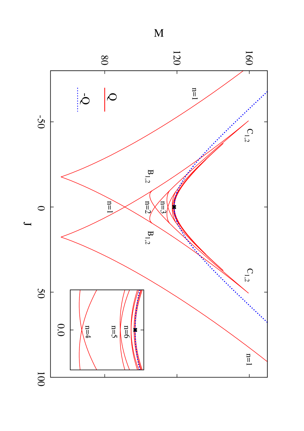
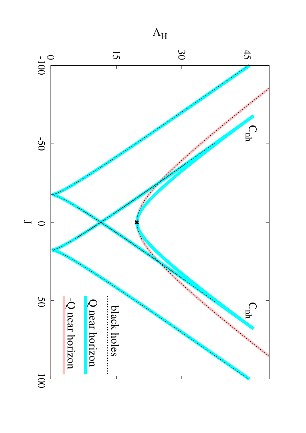
With increasing node number $n$, the mass $M_{n}$ converges monotonically from below to the mass of the extremal static black hole, $M_{\rm RN}$ (see Fig. 3). Surprisingly, however, the horizon area has the same value for all solutions of the sequence and the same holds for the magnitude of the horizon angular momentum. For comparison, we exhibit in Fig. 4 the area versus the angular momentum as obtained within the near horizon formalism for the same charge $Q$ (Figs. 2-6 are for a given value $Q=8\sqrt{3}\pi^{2}$; for completeness, the charge $-Q$ is also shown).

The set of near horizon solutions exhibits only three $J=0$ solutions, the extremal static one and two (symmetric) rotating solutions with lower area. The latter have precisely the values found for all solutions of the sequence. Thus these two near horizon solutions are not only associated with a single global solution each, but with whole sequences of global solutions.

Let us next address the full set of extremal solutions for fixed charge $Q$ inside the domain of existence. As expected, sequences of radially excited solutions [16] exist also for nonzero $J$. As seen in Fig. 3 two (symmetric) $n=1$ branches of solutions extend from the $n=1$ $J=0$ solutions up to a local minimum resp. maximum of the angular momentum. There cusps $C_{1,2}$ are encountered formed with higher mass $n=2$ branches. These higher mass branches then pass the $n=2$ $J=0$ solutions and end at bifurcations $B_{1,2}$ with the opposite $n=1$ branches.

Considering this same set of solutions in Fig. 4 we see, that the cusps $C_{1,2}$ encountered by the global solutions do not correspond to the cusps $C_{\rm nh}$ of the solutions obtained in the near horizon fomalism, since the branches of global solutions end before the branches of near horizon solutions end. Thus there are sets of near horizon solutions which do not possess counterparts in the sets of global solutions [17].

The bifurcations $B_{1,2}$ of the $n=2$ branches with the opposite $n=1$ branches are clearly visible in Fig. 5, where we exhibit the horizon angular velocity $\Omega_{\rm H}$ of the extremal solutions versus the angular momentum $J$. On the $n=2$ branches bifurcations $B_{2,3}$ with $n=3$ branches arise. Passing the $n=3$ $J=0$ solutions, these branches end in cusps $C_{3,4}$, formed with branches of the $n=4$ solutions. The $n=4$ branches pass the $n=4$ $J=0$ solutions and end in bifurcation points $B_{3,4}$ on the $n=3$ branches. This pattern then repeats again and again for the higher node branches.

In this way a whole sequence of branches is generated. Since the cusps $C_{n,n+1}$ occur at decreasing values of $|J|$, the number of extremal global solutions for fixed $|J|$ decreases with increasing $|J|$, whenever a cusp is passed. We conclude that a given near horizon solution can correspond to i) more than one global solution (possibly even an infinite set), ii) precisely one global solution, or iii) no global solution at all.

Interestingly, the presence of the bifurcation points $B_{n,n+1}$ indicates, that at each of these points there are two distinct solutions with the same global charges. They possess, however, different values of the area and thus correspond to different near horizon solutions.

Let us finally address the $\lambda$ dependence of the observed pattern of extremal solutions. This is shown in Fig. 6 where we exhibit the mass $M$ versus the CS coupling $\lambda$ of the rotating $J=0$ solutions with one to seven nodes. We note, that we do not find rotating $J=0$ solutions below $\lambda=2$, and the mass $M_{n}$ of the solutions with $n$ nodes approaches the mass $M_{\rm RN}$ of the static extremal solution, as $\lambda$ is decreased towards $\lambda=\lambda_{SG}$.

Further remarks.– The results in this work show that the intuition based on known exact solutions cannot be safely applied in the general case. Working in EMCS theory, we have shown that beyond a critical value of the CS coupling $\lambda$, for fixed charge $Q$, a sequence of branches of extremal radially excited black holes arises. To our knowledge, this is the first example of black holes with Abelian fields which form excited states reminiscent of radial excitations of atoms [19].

Also, these black holes clearly illustrate that the relation between the global solutions and the near horizon solutions may be rather intricate. Since there are near horizon solutions that do not correspond to global solutions, while other near horizon solutions correspond to one or more global solutions, possibly even infinitely many.

As we decrease the CS coupling below the critical value, this intriguing pattern of global solutions disappears. However, in the limit $\lambda\to 0$ when EM theory is obtained, we again encounter two branches of extremal solutions. The first branch is connected to the static RN black hole and has horizon area $A_{H}=\pi 3^{3/4}J^{2}Q^{-3/2}/\sqrt{2}+3^{1/4}\sqrt{2}Q^{3/2}/48\pi$. The second branch originates at the Myers-Perry solution, and has the rather unusual property to possess an entropy independent of the electric charge, $A_{H}=J/2$. Both branches are associated with near horizon solutions, that are only partly realized as global configurations.

Finally, we conjecture that extremal black holes with similar properties may also exist in other theories, in particular in a $D=4$ EM-dilaton theory.

Acknowledgement We gratefully acknowledge support by the Spanish Ministerio de Ciencia e Innovacion, research project FIS2011-28013, and by the DFG, in particular, the DFG Research Training Group 1620 ”Models of Gravity”. J.L.B is supported by the Spanish Universidad Complutense de Madrid.

References

- [1] A. Strominger and C. Vafa, Phys. Lett. B 379, 99 (1996) [arXiv:hep-th/9601029].
- [2] J. C. Breckenridge, D. A. Lowe, R. C. Myers, A. W. Peet, A. Strominger and C. Vafa, Phys. Lett. B 381, 423 (1996) [arXiv:hep-th/9603078].
- [3] J. C. Breckenridge, R. C. Myers, A. W. Peet and C. Vafa, Phys. Lett. B 391, 93 (1997) [arXiv:hep-th/9602065].
- [4] M. Cvetic, H. Lu and C. N. Pope, Phys. Lett. B 598, 273 (2004) [arXiv:hep-th/0406196].
- [5] Z. W. Chong, M. Cvetic, H. Lu and C. N. Pope, Phys. Rev. Lett. 95, 161301 (2005) [arXiv:hep-th/0506029].
- [6] J. P. Gauntlett, R. C. Myers and P. K. Townsend, Class. Quant. Grav. 16, 1 (1999) [arXiv:hep-th/9810204].
- [7] C. A. R. Herdeiro, Nucl. Phys. B 582, 363 (2000) [hep-th/0003063].
- [8] P. K. Townsend, Annales Henri Poincare 4, S183 (2003) [hep-th/0211008].
- [9] J. Kunz and F. Navarro-Lerida, Phys. Rev. Lett. 96, 081101 (2006) [hep-th/0510250].
- [10] J. Kunz, F. Navarro-Lerida and J. Viebahn, Phys. Lett. B 639, 362 (2006) [hep-th/0605075].
- [11] D. Astefanesei, K. Goldstein, R. P. Jena, A. Sen and S. P. Trivedi, JHEP 0610 (2006) 058 [hep-th/0606244].
- [12] H. K. Kunduri and J. Lucietti, JHEP 0712 (2007) 015 [arXiv:0708.3695 [hep-th]].
- [13] N. V. Suryanarayana and M. C. Wapler, Class. Quant. Grav. 24 (2007) 5047 [arXiv:0704.0955 [hep-th]].
- [14] We employ a collocation method for boundary-value ordinary differential equations, equipped with an adaptive mesh selection procedure [15]. Typical mesh sizes include points, the solutions having a relative accuracy of .
- [15] U. Ascher, J. Christiansen, R. D. Russell, Mathematics of Computation 33 (1979) 659; ACM Transactions 7 (1981) 209.
- [16] A family of radially excited solutions exists also in the non-extremal case for large enough values of , though with a finite maximal value of .
- [17] This feature was also found for extremal black holes in D=4 Gauss-Bonnet gravity [18].
- [18] C. -M. Chen, D. V. Gal’tsov and D. G. Orlov, Phys. Rev. D 78 (2008) 104013 [arXiv:0809.1720 [hep-th]].
- [19] This resembles also the case of black holes with non-Abelian gauge fields [20].
- [20] M. S. Volkov and D. V. Gal’tsov, Phys. Rept. 319 (1999) 1 [hep-th/9810070].