The Maximal Abelian Gauge in gauge theories and thermal monopoles for .
Abstract
We discuss and propose a proper extension of the Abelian projection based on the Maximal Abelian Gauge to gauge theories. Based, on that, we investigate the properties of thermal Abelian monopoles in the deconfined phase of the pure gauge theory. Such properties are very similar to those already found for , confirming the relevance of the magnetic component close to and the possible condensation of thermal monopoles as the deconfinement temperature is crossed from above. Moreover, we study the correlation functions among monopoles related to different subgroups, which show interesting features and reveal the presence of non-trivial interactions.
pacs
12.38.Aw, 11.15.Ha,12.38.GcI Introduction
An exact identification of the mechanism responsible for Color Confinement, and of the effective degrees of freedom relevant to it, is still missing. A commonly accepted scenario is that such degrees of freedom must be of dual, topological nature. A possible proposed mechanism is that based on dual superconductivity [1, 2], i.e. on the idea that the QCD vacuum is characterized by the spontaneous breaking of a magnetic symmetry, induced by the condensation of magnetically charged defects.
Possible approaches, followed to test this mechanism by lattice simulations, have either checked for the spontaneous symmetry breaking, by looking at the vacuum expectation value of magnetically charged operators and at the effective action of monopole configurations [3, 4, 5, 6, 7, 9, 10, 8], or have looked at the properties of monopole configurations extracted from non-Abelian configurations generated at equilibrium. The identification of Abelian degrees of freedom in non-Abelian gauge theories, and of Abelian monopoles in particular, relies on a procedure known as Abelian projection, which is based on the choice of an adjoint field. Since no natural adjoint field exists in QCD, that implies some arbitrariness. A popular choice is to perform the projection in the so-called Maximal Abelian gauge (MAG).
It is natural to expect that topological degrees of freedom, which are responsible for color confinement, play a relevant role also at and around the deconfinement transition. Indeed, magnetic monopoles evaporating from the low temperature magnetic condensate, which are usually known as thermal monopoles, have been advocated for their possible role in the properties of strongly interacting matter above the deconfinement transition [11, 12] Thermal monopoles are identified, in lattice QCD simulations at finite temperature, by looking for monopole currents with non-trivial wrappings in the Euclidean temporal direction [12, 13, 14]. Systematic lattice studies, regarding the properties of thermal monopoles in the deconfined phase of Yang-Mills theory have been performed in Refs. [15, 16, 17, 18, 19, 20, 21].
Results for the gauge theory have shown several interesting properties of such objects, which are compatible with a scenario in which the magnetic component of the Quark-Gluon Plasma plays a significant role right above the deconfinement temperature, while it is less relevant at asymptotically high temperatures, where the plasma is electrically dominated [22, 23]. In particular, spatial correlations of thermal monopoles show the presence of Coulomb-like, screened interactions among monopoles and antimonopoles [15], with an effective magnetic coupling which grows in the high regime [22], where the density of monopoles is also logarithmically suppressed with respect to the electric component. On the contrary, the coupling decreases approaching the low regime, and the analysis of the statistical distribution of trajectories with multiple wrappings in the temporal direction [24, 16] suggests that thermal monopoles may condense at a temperature which coincides, within errors, with the deconfinement temperature, giving further support to a confinement mechanism based on the condensation of magnetic charges.
The purpose of the present study is to extend such investigation to the pure gauge theory with three colors; preliminary results in the same direction have been reported in Ref. [25] and will be discussed in the following. The maximal Abelian subgroup of gauge theories is , hence the main change, when going to , is that various Abelian charges, i.e. various different species of monopoles, can be identified. On one hand, that makes a proper extension of the definition of the Maximal Abelian Gauge less trivial. On the other hand, new properties appear, associated with the interactions among different monopole species.
The paper is organized as follows. The extension of MAG to generic gauge groups will be discussed in detail in Section II. Numerical results obtained for thermal monopoles in the deconfined phase of will be presented and discussed in Section III. Finally, in Section IV, we draw our conclusions. Technical details and comparison among different definitions of MAG are reported in Appendixes A, B and C.
II Abelian projection and MAG monopoles in
In the following we shall review the definition of Abelian projection and of abelian magnetic monopoles in gauge theories. Then we shall focus on the Abelian projection defined by the so-called Maximal Abelian Gauge, discussing how the standard definition can be properly extended to . Even if some of the facts reported in this Section are already known from the literature, we report them here for the reader’s convenience.
II.1 Abelian projection and monopoles
Abelian projection is the procedure for identifying Abelian gauge symmetries within a non-Abelian theory. In the case of a gauge group, starting from a generic local field (with const.) transforming in the adjoint representation of the gauge group, one can define the Abelian ’t Hooft tensor [26]:
| (1) |
where, as usual,
and the generators are normalized as . The ’t Hooft tensor is, by construction, a gauge invariant quantity, which however depends on the choice of the adjoint field .
One can prove (see Refs. [27, 28] for a detailed discussion) that terms bilinear in and terms containing cancel in Eq. (1) in gauges where is a constant diagonal field, , and if is one of the fields
| (2) |
where , corresponding to the fundamental weights of the algebra. In such gauge (usually known as unitary gauge) reduces to a standard electromagnetic tensor,
| (3) |
where we have defined
| (4) |
as can be verified by exploiting the fact that is traceless. If is the diagonal part of the gauge field , then it is trivial to check that
where
is the matrix associated with the -th simple root. Hence the ’t Hooft tensor is the electromagnetic tensor associated to the subgroup generated, in the diagonal gauge, by .
In gauge theories, it is possible to identify independent subgroups, i.e. a maximal Abelian subgroup. The standard procedure [29] is to identify a local, hermitian operator transforming covariantly in the adjoint representation, , then fixing the gauge so as to make diagonal everywhere
| (5) |
That indeed fixes the gauge apart from a residual gauge symmetry. This is actually true only if a given ordering is also assigned for the eigenvalues , otherwise the residual invariance group contains also permutations. Since the eigenvalues are real, a standard possible choice [29] is
| (6) |
A ’t Hooft tensor can then be associated to each of the residual group, fixing in the diagonal gauge. can be chosen, without any loss of generality, to be a traceless operator, then can be written in terms of the matrices, which form a complete set over the Cartan subalgebra, as follows:
| (7) |
and making use of the relation we have
A special role is played by points where one of the coefficients in Eq. (7) vanishes, i.e. where two consecutive eigenvalues of coincide. Suppose for some , i.e. , then in the residual symmetry, corresponding to gauge transformations , is enlarged to the full invariance subgroup associated with the simple root . For that reason, the point represents a topological defect, where the gauge fixing procedure is not well defined. The projection of the operator over the -th subgroup vanishes in ; around , instead, one can choose either a hedgehog solution for it [26, 30] or, in the unitary gauge, a solution where is diagonal and the field contains the contribution from a Coulomb-like magnetic field centered around . In both cases we identify as the location of a magnetic monopole, relatively to the corresponding subgroup, where the Abelian and the non-Abelian Bianchi identities are violated [31].
In the particular case of , which is the subject of our numerical study, one can identify two different Abelian monopole species which manifest themselves, in the unitary gauge, by the presence of a Coulomb-like magnetic field in the corresponding Abelian gauge fields
| (8) |
II.2 Abelian projection and monopoles on the lattice
Let us now discuss how that applies to the lattice formulation of non-Abelian gauge theories, a topic first studied in Ref. [32]. The Abelian projection is defined, as in the continuum, in terms of a local operator , living on lattice sites , transforming in the adjoint representation. Differently from the continuum case, however, ambiguities emerge when defining the ’t Hooft tensor and the Abelian gauge fields in the unitary gauge, where is diagonal. Gauge links , which are the elementary lattice variables, are related to the gauge field by the following relation, , which is valid in the continuum limit. The procedure of taking the diagonal part of the gauge field can be implemented on the lattice by taking the diagonal part of gauge links ; however one can also take the diagonal part of the product of two or more elementary link variables: that leads, due to the non-Abelian nature of the theory, to alternative definitions of the Abelian projected fields, which differ by terms. However, such ambiguities disappear as the continuum limit is approached.
In the following we shall take, as usual, the prescription of starting from the elementary link variables: after gauge fixing we take the phases of the diagonal part of each gauge link , as specified in details in Appendix B, then we construct the Abelian gauge phases , following Eq. (4), as
| (9) |
and finally the -th ’t Hooft tensor (Abelian plaquette) is constructed as
| (10) |
Regarding the location of magnetic monopoles, it is clear that the recipe of locating points where one of the coefficients vanishes, i.e. where two consecutive eigenvalues of coincide, cannot be implemented on a discrete space-time. It is however possible to locate them, in the unitary gauge, as the points from which a net magnetic flux comes out. This is implemented in the standard De Grand-Toussaint construction [33], which looks at the net flux coming out of elementary three-dimensional lattice cubes. In particular, monopole currents of a given type are defined as
| (11) |
where is the lattice derivative and is the compactified part of the abelian plaquette phase
| (12) |
II.3 Maximal Abelian Gauge and magnetic monopoles in gauge theories
The location of monopole currents depends on the choice of the Abelian projection. A standard, popular choice, is to define Abelian projection based on the so-called Maximal Abelian Gauge (MAG). For , MAG is defined as the gauge for which the following functional
| (13) |
has a maximum and in Ref. [34] this definition was used for the first time in a numerical study. It can be shown by explicit calculation that is proportional, apart from a constant term, to the sum of the squared diagonal element of the gauge links,
| (14) |
and that, at the same time, on stationary points of the traceless and hermitean operator is diagonal and can be related to the local operator which defines the Abelian projection. In particular, only on MAG fixed configurations, takes the following explicit expression in terms of the gauge links
| (15) |
while in a generic gauge, connected to MAG by the local gauge transformation , it is defined as , which makes it a local adjoint operator by construction. Notice that this means that the explicit form of the adjoint field is not known apriori, but only after MAG has been fixed.
The usual rationale behind the use of the MAG projection is that, since the sum of the squared diagonal elements is maximized, abelian projected fields retain most of the original Yang-Mills dynamics (Abelian Dominance). On the other hand, such choice is supported by the empirical fact that the physical properties of MAG monopoles show a negligible dependence on the lattice ultraviolet (UV) cutoff. An important property of the Maximal Abelian Gauge is that magnetic currents, defined through the violation of the non-abelian Bianchi identities, are correctly identified and magnetic charge obeys the correct Dirac quantization condition [31] (see also Ref. [35] for a related numerical study). In view of this, in the following we shall adopt the Maximal Abelian Gauge. However, the extension of the definition to the generic gauge group reveals ambiguous and various possibilities exist: in the following we shall discuss which of them are suitable for a correct definition of magnetic charges, in the light of the arguments given in Sections II.1 and II.2.
A possible, straightforward generalization for , introduced in Ref. [36] and usually adopted in the literature [37, 38, 39, 40], is to maximize the sum of the squared diagonal elements of all gauge links. The corresponding functional, in the case of , reads:
| (16) | |||||
where and . This extension seems ideally suited for studies regarding Abelian dominance, however it has the problem that no natural operator exists, transforming in the adjoint representation, which is diagonal in this gauge, therefore it does not seem to be well suited for an extension of MAG Abelian projection to . We will discuss in more detail the problem later in this Section.
An alternative possibility, suggested for in Refs. [41, 42, 43] (where it is called “generalized MAG”), is the following
| (17) |
where is a generic element of the Cartan subalgebra. For appropriate choices of , the maximization of the functional in Eq. (17) defines the following diagonal operator:
| (18) |
Suppose indeed that we have reached an extremum for , then its variation for any infinitesimal gauge transformation must vanish. Let us take a particular transformation which is non-trivial in a single site, , then the extremum condition reads:
| (19) |
A non-trivial condition on applies if is not in the Cartan subalgebra, in particular, taking alternatively and , we obtain (no summation over repeated indices is intended)
| (20) |
which implies for every , unless . Therefore is diagonal if has no pair of coinciding eigenvalues. If is expanded over the basis of fundamental weights (see Eq. (2))
| (21) |
such condition reads
| (22) |
for any , which implies various constraints, including the fact that none of the can vanish. Such constraints can be better specified if we now require a given ordering for the eigenvalues of the diagonal operator , for instance the one in Eq. (6), at least around the perturbative vacuum, where and . That implies , hence, from Eq. (22), we obtain that .
Following the discussion in Sections II.1 and II.2, magnetic monopoles of type will be located at points where the coefficient vanishes in the expansion ; each monopole species will be associated to a particular residual subgroup. For configurations which are close to the perturbative vacuum, , we have , hence no monopole will appear in any subgroup, since ; the appearance of a monopole therefore requires a non-perturbative fluctuation of gauge fields, as it is naturally expected. These considerations lead us to fix a well defined choice for , that will be adopted in the following: while no particular reason exist to put further constraints on , apart from , it is clear that a choice for which all coefficients are equal treats all monopole species symmetrically, hence it seems preferable. Therefore we will fix for every , ending up with the following definition of
| (23) |
To better appreciate such choice, consider that, in case one of the coefficients is much smaller than the others, than the appearance of a monopole-like defect in the corresponding subgroup may be induced also by small scale fluctuations, leading to possible ambiguities, especially in a lattice setup where one would like to distinguish true non-perturbative fluctuations from artifacts at the UV scale. That also clarifies the advantage of the Abelian projection based on MAG, with respect to other possible projections. Consider, for instance, the Abelian projection based on the diagonalization of the plaquette operator, taken, e.g., in the plane:
| (24) |
In the limit of small fields, , we have
,
meaning that for every . Hence we expect that
the Abelian projection based on the plaquette operator will detect
many magnetic monopoles even in the limit of small fields: in this
case the detection procedure will be strongly affected by lattice artifacts,
i.e. by UV noise, leading, e.g., to a wrong scaling of the monopole density
in the continuum limit. The same argument applies to any other Abelian
projection based on a local adjoint operator vanishing in the limit of
small gauge fields.
Finally, let us summarize and further clarify the reasons leading us to the proposed extension of MAG projection for gauge theories and to discard other possibilities considered in the literature, like that based on the functional in Eq. (16). The original aim of Abelian projection is to fix the non-abelian gauge symmetry apart from a residual maximal Abelian subgroup, to which electric and magnetic charges can be associated. The need for fixing the subgroups simultaneously, i.e. by the same gauge condition, stems from the requirement that each electric or magnetic charge be neutral with respect to all other subgroups.
¿From this point, it may seem that fixing the gauge by looking for a maximum of the functional in Eq. (16) may work equally well, even if no diagonal operator is naturally associated to such a choice. Indeed, the functional is invariant under gauge transformations belonging to the maximal subgroup, which is therefore well defined on each stationary point of the functional. However, the crucial point is that must be the only residual symmetry, i.e. one should take care of fixing any possible additional symmetry, like that under index permutations.
The functional in Eq. (17), on which our choice of Abelian projection is based, is in general not invariant under local permutations of the color indexes, , which transform gauge links as follows: . Indeed, it is easily verified that such transformation is equivalent to performing a local modification of , corresponding to a permutation of its diagonal elements, , which changes the value of the functional.
The operator in Eq. (16) is not invariant under local permutations as well, since in general they change the identification of the diagonal elements. However, global permutations, i.e. with independent of , are a residual symmetry of such operator. Such residual symmetry, unfortunately, makes it ambiguous to identify in which subgroup a given magnetic monopole appears. A direct consequence, that will be verified numerically in the next subsection, is that when one constructs magnetic currents according to the abelian projected phases in such a gauge, magnetic monopoles appear simultaneously on the same site and in different subgroups, meaning that the magnetic charge operators are not well identified, i.e. they do not commute with each other.
Actually, the particular choice adopted for in Eq. (23), has a global symmetry as well, corresponding to the following global permutation: , i.e. to the inversion in the location of all eigenvalues of . However, such residual symmetry is harmless, since it sends pairs of adjacent eigenvalues into pairs of adjacent eigenvalues, hence it changes the location of the subgroups, but leaves them still well identified.
II.4 Implementation for and the detection of independent monopole species.
In the following we will apply the above considerations to the study of magnetic monopoles in the pure gauge theory. To summarize, our procedure for Abelian projection will be to fix the gauge by maximizing the functional
| (25) |
Then we take the diagonal part of gauge links, , and determine the Abelian phases , corresponding to the two residual subgroups, following Eq. (9), which for reads and (remember that ). The numerical algorithm adopted to maximize the functional in Eq. (25) and that used to extract are illustrated respectively in Appendix A and B.
Starting from and , we determine the two monopole currents and , following the De Grand-Toussaint method [33] (see Eqs. (11) and (12)). Monopole currents form closed loops, since , and we will be interested in particular in monopole loops with a non-trivial wrapping around the Euclidean temporal direction, which can be identified with thermal monopoles [12, 13, 14, 15], and whose properties in the deconfined phase of gauge theory will be studied in Section III.
It is interesting to write down a continuum expression for the functional in Eq. (25). A straightforward computation yields, apart from a constant term,
| (26) |
which in the continuum limit, , becomes
| (27) |
If we adopt the usual notation , where are the Gell-Mann matrices, we obtain
| (28) |
the Higgs field defining the Abelian projection is oriented like in the gauge fixed configuration (see also Ref. [41] for a derivation in the case of a more general choice for ). For comparison, we report also the continuum expression corresponding to the standard extension of MAG to , Eq. (16),
| (29) |
whose maximization corresponds to the minimization of the non-diagonal part of the gauge field, but has no Higgs field associated with it.
To conclude the present Section, and before starting a detailed study of thermal monopole properties, we would like to discuss numerical data showing that our choice of Abelian projection indeed leads to independent monopole currents. In order to give a quantitative measure of such “independence”, let us call () the probability that a given three-dimensional cube of the lattice is pierced by monopole current (), and by the probability that the cube is pierced both by current and current . If the two monopole currents were completely independent of each other, than one would expect
| (30) |
i.e. the probability of two coinciding currents should be equal to the product of the respective probabilities. Actually, even if the two magnetic charges are independent, each of them being neutral with respect to the group of the other charge, we still expect some correlations of physical origin, which is due to interactions induced by the non-Abelian degrees of freedom: such interactions will be studied in more detail in Section III, where we analyze spatial correlations among thermal monopoles. In any case, even considering such interactions, the probability of having two different monopoles exactly on the same lattice cube should not be particularly enhanced, especially when, approaching the continuum limit, the volume of the single cube shrinks to zero. Therefore the ratio in Eq. (30) should stay of .
We have studied the ratio reported in Eq. (30) for the pure gauge theory, with the Wilson (plaquette) action discretization, on a lattice, for a few values of the inverse gauge coupling and for different choices of the monopole currents, and . Results are reported in Fig. 1. The first choice corresponds to the two independent monopole currents identified by the definition of MAG adopted in the rest of this study, see Eq. (25): the ratio is for all explored values of , as expected for independent currents.
It is interesting to notice that, even in this gauge, if the second current is constructed making use of the wrong abelian phase, for instance taking , such property is completely lost and the ratio in Eq. (30) is of the order of - : in the gauge specified by Eq. (25) such phase receives contribution from both subgroups, hence it defines a magnetic current which strongly overlaps with both correct currents. As a matter of fact, if one of the two correct monopole currents pierces a given lattice cube, there is a probability larger than 50% that a monopole current, corresponding to the fake abelian phase, is found on the same cube.
Last choice corresponds to the gauge fixing specified by the functional in Eq. (16) and to the currents associated again to and . The overlap between the two currents is clearly visible, with of the order of - over the explored range of ’s. The probability that a monopole current of a given type is found in a cube where another current type has already been found is of the order of 20-30% over the whole range of explored values. In this case, similar results are obtained considering any pair of abelian phases, since all diagonal elements are treated symmetrically.

A final comment regards the problem of gauge fixing ambiguities. It is well known that functionals like those in Eqs. (16) and (17) possess many local maxima, corresponding to different gauge fixed configurations, i.e. different Gribov copies. A usual choice, in order to fix the gauge unambiguously, is to define it as that corresponding to the global maximum of the functional, even if finding it may result computationally expensive. Such strategy is well justified for the functional in Eq. (16) and for questions related to Abelian dominance, i.e. regarding the possibility of reproducing physical properties of the non-Abelian theory by the diagonal part of gauge fields only.
In the case of our interest, however, every local maximum of the functional in Eq. (17) will lead to a well defined diagonal operator , hence to a legitimate Abelian projection, on the same footing with other Gribov copies, including the global maximum of the same functional. Different Gribov copies will lead to different adjoint operators , hence to different Abelian projections and different monopoles. In that sense, numerical studies which look for the global maximum of the MAG functionals can be considered as an important tool to reveal the systematic uncertainties linked to such choice.
Taking the Gribov copy which is found first by the maximization procedure, starting from the original configuration sampled by the Monte-Carlo algorithm, can be considered as a practical criterion which leads to a correct behavior of the monopole properties in the continuum limit [15]: we will follow such prescription in our study of thermal monopoles for . Accurate studies have been performed for thermal monopoles, adopting simulated annealing procedures in order to get as close as possible to the global maximum of the MAG functional [44, 18, 19]: apart from a 20% difference in the overall density of thermal monopoles, no other significant differences have been revealed, regarding the main physical properties of thermal monopoles.
It would be interesting, in future studies, to consider the implementation for gauge theories of different gauge conditions which, while sharing with the MAG the property of being safe from ultraviolet fluctuations, are also free of Gribov copy ambiguities. One possibility could be the so-called Laplacian gauge, see Refs. [45, 46].
III Numerical simulations and results
Monopole currents form closed loops, which may wrap by periodicity around the lattice torus. While in the confined phase wrappings in both spatial and temporal directions take place, usually associated to the presence of a large, percolating cluster of currents, in the deconfined phase the non-trivial wrappings survive only in the Euclidean, periodic time direction, which is associated to the thermal properties of the theory.
Such trajectories with non-trivial temporal wrappings can be associated with thermal objects populating the finite medium [13, 14, 12], in analogy with the path-integral representation of the partition function of a system of quantum particles. For that reason they have been directly related to the magnetic component of the deconfined plasma [12], constituted by thermal abelian monopoles evaporating from the low magnetic condensate. Many properties of thermal monopoles have been studied in subsequent works [15, 16, 17, 18, 19, 20, 21], which are of interest for the comprehension of the deconfined state of Yang-Mills theories and of the confinement/deconfinement mechanism itself. Such studies will be extended to in the present Section.
We summarize the main steps for identifying thermal monopoles on a given gauge configuration. We first look for monopole currents piercing a given time slice of the lattice (e.g. , at ) in the temporal direction, then we follow the current around the lattice and keep trace of the number of temporal wrappings the current makes before going back to the original detection point. Currents wrapping in the positive (negative) direction are associated to monopoles (antimonopoles). If the current wraps only one time, then the spatial location of the thermal monopole on the starting time slice is well defined, apart from possible ambiguities at the UV scale, due to short range fluctuations of the trajectory. If the current wraps 2 or more times, then it can be associated to 2 or more thermal monopoles undergoing a cyclic permutation as they go around the thermal cycle: such trajectories are typical of the path integral representation of a system of identical, bosonic particles. Possible ambiguities in the identification procedure described above can occurr when two trajectories cross at the same point: it is not clear if they represent a single trajectory with a double wrap or not; however, from a practical point of view, the presence of two currents in the same lattice cube is very rare event, hence of no statistical significance.
In the following, we will show and discuss numerical results obtained by simulating with the Wilson plaquette action (making use of a standard combination of heat-bath [47] and over-relaxation [48] updates). The temperature has been tuned both by changing the number of temporal lattice sites, , at fixed UV scale (with ranging from 4 to 11) and by tuning the inverse bare coupling at fixed . A number of different spatial sizes have been explored, ranging from to . In order to obtain the physical value of the temperature, in units of , we have exploited the non-perturbative determination of and the critical values for various values of reported in Ref. [49]. For each parameter set we have measured thermal monopole properties on a number of decorrelated gauge configurations ranging from a few hundreds up to a few thousands.
A first quantity that we will look at is the total density of thermal monopoles as a function of . Results for show that the density increases with , as expected for a particle-antiparticle gas, but with a typical logarithmic suppression which can be related to the temperature behavior of the magnetic coupling and shows that monopoles degrees of freedom become irrelevant, with respect to gluons, in the high , perturbative regime, while their role is more and more significant as the deconfining temperature is approached from above.
Further information will be obtained by looking at the density of trajectories with multiple wrappings. As discussed above, such trajectories can be interpreted in terms of the exchange of identical particles: they are strongly suppressed at high , where the system is quasi-classical, and become statistically relevant at low . The analysis of Ref. [16], which is based on the analogy with a free boson gas, has shown that for the distribution of multiple wrapping trajectories as a function of can be used to detect the point where thermal monopoles seem to condense, and that such point coincides within errors with , giving support to a confinement mechanism based on the condensation of magnetic charge (dual superconductor mechanism). The same analysis will be repeated for in Section III.2.
Finally, in Section III.3, we will analyize the spatial correlations among thermal monopoles. Already in , where a single monopole species exists, such correlations furnish interesting information, showing the presence of Coulomb-like, screened interactions among monopoles and antimonopoles, with an effective magnetic coupling which grows with . For , apart from verifying the presence of analogous interactions among monopoles and antimonopoles of the same kind, we will have the possibility of investigating the correlations between the two different species, which are related to the non-Abelian nature of the theory and will reveal to be highly non-trivial.
III.1 Monopole density

We define the total density of thermal monopoles of a given species as [12, 13, 14]
| (31) |
where is the winding number in the temporal direction of the monopole current initially detected at the lattice site , the sum is over all spatial sites at a given time slice and is the spatial volume.
It is convenient to define the following dimensionless ratio
| (32) |
which for a gas of free quantum particles and antiparticles of mass should tend to a constant as .
In Fig. 2 we show for the first monopole species and for different temperatures and lattice spacings, results obtained for the second species are compatible within errors, as expected from our choice of in Eq. (25). For comparison, we also report data obtained for in Ref. [15]. We notice a good scaling to the continuum limit. Data for seem to stay slightly below the ones, however it is important to stress that the comparison is made at fixed and that is about 10% higher for than for : if data were compared at fixed , where is the string tension, they would be practically coincident. Therefore, seems to reach slightly higher values, around , for than for , but just because is lower for and is a decreasing function of .

The dependence of on is best appreciated from Fig. 3, where the densities of both monopole species are shown over an extended temperature range. It is clear that does not approach a constant behavior, so that, like for [15], a description of thermal monopoles as a gas of free particles is not appropriate, even at asymptotically high , in agreement with a scenario based on the electric-magnetic duality [11], according to which the high phase of Yang-Mills theories is electrically dominated, while the magnetic component is strongly interacting.
Explicit predictions can be done for , based on perturbative and dimensional reduction considerations, leading to a behaviour proportional to [50, 11], where is the renormalized running coupling, hence a reduction factor for , with respect to the free massless particle case, of the order of , where is some effective scale. Based on such prediction, we have tried to fit data11 1 Reported fit values have been obtained for the first monopoles species, but results for the second species are completely equivalent. in Fig. 3 according to
| (33) |
If we consider only and fix , we obtain , and . If we instead leave as a free parameter, we get and , in very good agreement with the perturbative prediction.
Finally, we would like to make a direct comparison with the results obtained by adopting the standard extension of MAG to based on the functional in Eq. (16), like in Ref. [25]: that does not permit a proper distinction between the two monopole species, it is however interesting to compare the overall densities. In Fig. 4 we report the ratio of thermal monopole densities, as a function of , obtained on our sample of thermalized configurations in the two cases: the gauge fixing procedure is similar, in particular for both functionals we stop on the local maximum which is first found when starting from the Monte-Carlo thermalized configuration. Results obtained adopting the functional in Eq. (16) are consistently lower, by 10-30%, over the whole range of explored temperatures: this is consistent with the results presented in Ref. [25], which are based on Eq. (16) and provide evidence for a thermal monopole density in lower than that obtained for , while our results show instead that they are practically equal.

III.2 Monopole condensation
Trajectories with multiple temporal wrappings can be related to the nature and properties of monopoles as identical quantum particles, as follows from the interpretation of the set of monopole trajectories, extracted from a given gauge field, as a possible configuration of the Euclidean path integral of an ensemble of identical particles. Indeed, the path integral of identical particles at thermal equilibrium is made up of path configurations which are periodic apart from a possible permutation of the particles, meaning that each configuration presents in general closed paths, with and the -th path wrapping times, in such a way that : such configuration corresponds to a permutation made up of cycles of sizes .
When effects related to quantum statistics are negligible, i.e. when the system is close to the Boltzmann approximation (like it happens, for example, at high ), configurations deviating from the identical permutation have a negligible weight in the path integral, so that trajectories presenting multiple wrappings are very rare. Their statistical weight is instead expected to increase as quantum effects become more important, and in a well defined, critical way as one approaches typical phenomena like Bose-Einstein Condensation (BEC). A treatment of BEC-like phenomena by a path-integral approach goes back to the seminal papers by Feynman [51, 52], where a path integral formulation was applied to describe the superfluid transition in 4He.

In particular, for a set a free bosons of mass , one finds that the density of paths wrapping times (-cycles) is given by (see, e.g. , Refs. [53, 16])
| (34) |
where is the number of -cycle in one configuration, is the De Broglie thermal wavelength, and the dimensionless quantity is related to the usual chemical potential for free bosons by , with the constraint (i.e. ). As , i.e. as the system approaches BEC, higher -cycles become more and more frequent and the exponentially suppressed behavior of turns into a critical power law behavior.
In Ref. [16], the distribution of monopole trajectories wrapping times has been used, in combination with a simple ansatz like that in Eq. (34), to extract for the thermal monopoles in the gauge theory and infer that they undergo condensation at a temperature which coincides, within errors, with the deconfinement temperature . We would like to repeat a similar analysis for .
In Fig. 5 we report , the density of trajectories wrapping times, normalized by , as a function of for a few values of . Results have been obtained on a lattice. It is evident that, for each , the relative weight of rapidly increases as is approached from above. Moreover, for each data can be nicely fitted according to the simple ansatz in Eq. (34), as it happens in the case, giving us access to the effective chemical potential .

The effective chemical potentials, obtained in this way over an enlarged set of temperatures above , are displayed in Fig. (6). We report results from two different lattices, and , in order to show that the scaling to the continuum limit holds within errors. As a second step, following Ref. [16], we have tried to fit according to a critical behavior:
| (35) |
obtaining (all data are included) , and , with .
We conclude that also in the pure gauge theory, if one interprets thermal monopole trajectories as paths describing the quantum properties of a thermal particle ensemble, there is clear evidence for such ensemble to undergo BEC-like condensation exactly at . Notice that for , since the transition is first order, the coincidence of the transition temperature with extrapolated from the critical behavior as in Eq. (35) is not expected apriori; in particular one could expect that the transition takes place before actually goes to zero, i.e. that . However, since the transition is a weak first order transition, it may still be that the two temperatures coincide within errors. It will be interesting, in this respect, to repeat the same analysis for gauge theories with , where the first order transition gets stronger.
III.3 Monopole interactions
The spatial distribution of thermal monopoles at a given Euclidean time slice gives information about the mutual interactions of those objects. In particular, one can study the density–density correlation function between any couple and of thermal monopole species, which can be determined as the ratio between the probability of having a monopole of kind at distance from a given reference monopole of kind , and the same probability in case the monopole locations are completely uncorrelated and randomly distributed, i.e.
| (36) |
where is the number of monopoles in a spherical shell of thickness at distance from the reference monopole of kind ; in order to minimize artifacts related to the lattice geometry, we have used, in place of , the actual number of lattice sites contained in the shell.
A value () indicates that at distance we have less (more) particles than expected in a non-interacting medium, i.e. there is a repulsive (attractive) interaction. The determination of such correlation functions for has shown the existence of screened Coulomb-like attractive (repulsive) interactions between monopoles and antimonopoles (monopoles) [15, 19], with a strength which grows with the temperature, in agreement with expectations based on the electric-magnetic duality [11].

For , we have determined the correlation functions for three values of , where we have collected larger statistics (up to a few thousands decorrelated configurations). For we have performed simulations on two different lattice sizes and values ( at and at ), in order to check also for continuum limit corrections, while for and we have performed simulations at a single lattice spacing ( and lattices at and ). We have chosen the shell thickness to be lattice spacing in all cases.
In Fig. 7 we show correlations between monopoles and antimonopoles of the same species and for the three highest values of . Data for are reported separately in Fig. 10, to better appreciate the good scaling to the continuum limit. Results are qualitatively very similar to those obtained for ; a qualitative agreement is also found with the results for monopole-monopole interactions reported in Ref. [25], which are based on the functional in Eq. (16). As for we can try to obtain information about the interaction potential by looking at the large distance region, where
| (37) |
In , a screened Yukawa potential,
| (38) |
fits well numerical data, therefore we have tried a similar ansatz also for .
An important question is whether we can describe both monopole-monopole and monopole-antimonopole interactions by the same (opposite) magnetic coupling , i.e. if the interaction among monopoles and antimonopoles is Coulomb-like. The answer is that if we try separate fits to monopole-monopole and monopole-antimonopole correlations, different values of are obtained, however it is possible to perform a common fit, assuming that the coupling is the same, obtaining values of which are marginally acceptable; fit results are reported in Table 1. The fitted magnetic coupling shows a slowly increasing behavior as increases, in fair agreement with results and with arguments based on the electric-magnetic duality [11]; values obtained for are also in rough agreement with the results reported in Ref. [25]. The screening length shows a sizable decrease as increases. The plasma parameter, , stays always well above 1, indicating a strongly interacting behavior of the thermal monopole plasma.
| 1.333 | 3.1(4) | 0.285(11) | 52/36 |
| 2 | 4.3(5) | 0.209(6) | 48/39 |
| 3 | 5.9(5) | 0.151(3) | 48/41 |
| 4.86 | 6.4(6) | 0.114(3) | 47/41 |

Finally, a new, non-trivial aspect of , with respect to , regards the correlations among monopoles of different species, and . Those are shown in Fig. 8 for two values of . Correlations looks very similar to those among monopoles of the same species, however the sign of the interaction is opposite, with attraction between monopoles and repulsion between monopoles-antimonopoles of different species. This is not surprising, if we recall that the magnetic charge operators of each species are proportional to the corresponding roots, i.e. , for , to and , and that the mutual, Coulomb-like interaction between monopoles of different species must be proportional to the scalar product of the corresponding charges [54], i.e. to , while in the case of monopoles of the same species the corresponding product is proportional to .
That suggests that, apart from the minus sign, we should be able to see also a factor in the corresponding coupling. However, new, unexpected features of the correlation functions make a fit according to Eq. (38) unfeasible. Indeed, a more careful observation shows that, after the first positive peak in , a small, negative well develops for , corresponding to repulsive interaction at intermediate distances; the opposite behavior is visible also in the monopole-antimonopole correlation, . All that is better visible in Fig. (9), where the interesting intermediate region has been magnified.
An oscillating behavior of the density correlation function is typical of systems with non-trivial, e.g. liquid-like, properties. A possible explanation, for instance, could be that monopoles of different species are bound into larger objects (think, for instance, of calorons and of their monopole constituents), and that such larger objects undergo weak repulsion, thus explaining the inversion at intermediate distances. It is interesting to notice that, reasoning along the same lines of Ref. [55], the possible formation of bound states between monopoles of different species may explain the lower values of which are needed to reach confinement (monopole condensation) in with respect to . All that claims for more careful future studies and, in particular, for an extension to larger () gauge groups, where the pattern of interactions could be even more interesting and reveal fundamental aspects of Yang-Mills theories.

Correlations among different species are reported in Fig. 10 as well, where data for obtained at two different lattice spacings are compared, showing a very good scaling to the continuum limit, apart from small deviations in the short distance region, i.e. at the scale of the UV cutoff.

IV Conclusions
The purpose of the present study has been that of extending the investigation of thermal monopoles properties to the theory with 3 colors. As a first step in this direction, the extension of the Maximal Abelian projection to gauge theories with has been discussed.
We have shown that extensions usually adopted in the literature, based on the maximization of the diagonal components of gauge links, may not lead to a proper identification of the different monopole species. Instead, inspired by previous suggestions from the literature [41, 42, 43], we have proposed and implemented an extension which has still a well defined Higgs field associated with it and identifies a strict residual symmetry, leading to a proper detection of independent monopole species.
Based on that, we have presented various results regarding the properties of thermal monopoles in the deconfined phase of the pure gauge theory. Most properties are very similar to those of monopoles, including the density of both monopole species and the distribution of trajectories with multiple wrappings, which indicate condensation of both monopole species at the deconfinement transition.
Spatial correlations of thermal monopoles, instead, present new, interesting features. Correlations among monopoles of the same species still indicate the presence of a screened, Coulomb-like interaction, with a magnetic coupling which increases with . New interactions however appear: monopoles of different species attract each other, while monopole - antimonopole pairs repel, in agreement with the structure of their charge operators within the group. Moreover, spatial correlation functions among monopoles of different species show a clear oscillating behavior, with secondary long range structures, which indicate the presence of non-trivial, e.g. , liquid-like, properties, and may be related to the formation of monopole-monopole bound states. It is tempting, in view of that, to associate thermal monopoles with caloron constituents carrying fractional topological charges [56], and to make a direct connection between the condensation of thermal monopoles and the drastic change, at the phase transition, in the dependence of the theory on the topological parameter [57, 58, 59, 60, 61, 62]. All that claims for a further extension of the present study to gauge theories, with , where the pattern of interactions is expected to be even more interesting, and, of course, to QCD.
Acknowledgments
We thank A. Di Giacomo, E. Shuryak and A. Zhitnitsky for many useful discussions. We acknowledge the use of the computer facilities of the INFN CSNIV cluster in Pisa.
Appendix A Gauge Fixing Algorithm
The algorithm for the maximization of the functional in Eq. (17) follows closely that commonly used in the case, i.e. a combination of local maximization-overrelaxation, which we briefly review in the following.
If we perform a gauge transformation which is non-trivial only in one lattice site , , then the part of the functional in Eq. (13) which depends on is
| (39) |
where is defined in Eq. (15). It is easy to find the element maximizing the expression (39). , as any element, can always be written in the form
and the expression in Eq. (39) is independent of . Hence, without loss of generality, we can parameterize as follows
| (40) |
so that
is a traceless adjoint operator, i.e. one can write , hence
| (41) |
Last expression has a maximum when the unit vector is parallel to , hence
| (42) | ||||
The gauge-fixing algorithm consists of sweeps of one-site gauge transformations which locally maximize the MAG functional; the algorithm is stopped when the adjoint operator turns out to be diagonal within a given precision, i.e. when the average squared modulus of the non-diagonal contribution, , where is the lattice volume, goes below a given threshold. The algorithm can be accelerated by using overrelaxation [48, 63], i.e. by choosing
| (43) |
a value reveals to be optimal.
Let us now switch to the general functional defined in Eq. (17). In this case, inspired by the Cabibbo-Marinari algorithm for heat-bath updating in [47], we will adopt a procedure of local maximization over subgroups. Let us consider again a gauge transformation which is non-trivial only at site and suppose further that is non-trivial only in the subgroup corresponding to rows and colums and (). The functional to be maximized by is
| (44) |
Also in this case one proves that, if the expression of is , then is irrelevant and one can ignore it. Therefore we fix
We have that for or outside the given subgroup, while for both and inside it has the form:
| (45) |
Regarding , we can always parameterize its restriction to the subgroup as follows
| (46) |
hence
| (47) |
where is a constant. If the eigenvalues are ordered, as we have assumed in Section II.3, then and the solution for the local maximum over the chosen subgroup is obtained exactly as in Eq. (42), otherwise a global minus sign would apply, . Overrelaxation also proceeds as in Eq. (43): we have found that a coefficient similar to that used for , , is optimal also in the case. The local overrelaxation is repeated iteratively over all possible subgroups and over all lattice sites. The algorithm is stopped when the average of the squared moduli of the non-diagonal elements of goes below a given threshold, which has been set to .
The maximization of the functional in Eq. (16) can be performed locally over the subgroups as well. Let us consider a gauge transformation belonging to the first subgroup, and 2, at first: in this case, since the term is invariant under such gauge transformations, everything goes exactly as specified previously with . On the other hand the functional in Eq. (16) is symmetric over the subgroups, hence one can use exactly the same procedure for all subgroups. As we have stressed above, no diagonal local adjoint operator is naturally associated with this version of the maximal abelian gauge. Anyway one can prove that, when a maximum of the expression (16) is reached, each of the operators , and , defined as in Eq. (15) with and respectively, is diagonal when restricted to the corresponding subgroup, i.e. one has
| (48) |
for each site (see, e.g. , Ref. [41]). Such condition can be taken as a stopping criterion in this case.
Appendix B Extraction of the diagonal part of gauge links
For the gauge theory, the extraction of the Abelian phases, i.e. the degrees of freedom related to the residual invariance gauge group, coincides with taking the phases of the diagonal elements of the gauge links.
In the procedure is less trivial. Indeed, writing the diagonal element of the generic matrix in the form , it is not guaranteed that belongs to , since, in general, with .
One simple procedure, adopted in some studies [40], is to define an diagonal element with and extracting the Abelian phases from it. A more accurate procedure [41] is instead to project the original element onto the closest diagonal element by maximizing
| (49) |
Here we present an approximate but quite simple and accurate procedure to get the maximum. It is easy the check that, due to the constraint , the condition for stationary points of is to have
| (50) |
On the other hand, for links of gauge fixed configurations, usually is a small quantity and on the maximum we expect , so that we can approximate and obtain the following solution to Eq. (50)
| (51) |
The extraction of the Abelian phases then proceeds as specified in Eq. (9).
Appendix C Dependence of results on the choice of
Even if the choice made in Eq. (23), i.e. of treating all monopole species symmetrically, is the most natural, it is interesting to understand what are the effects of a different choice of .
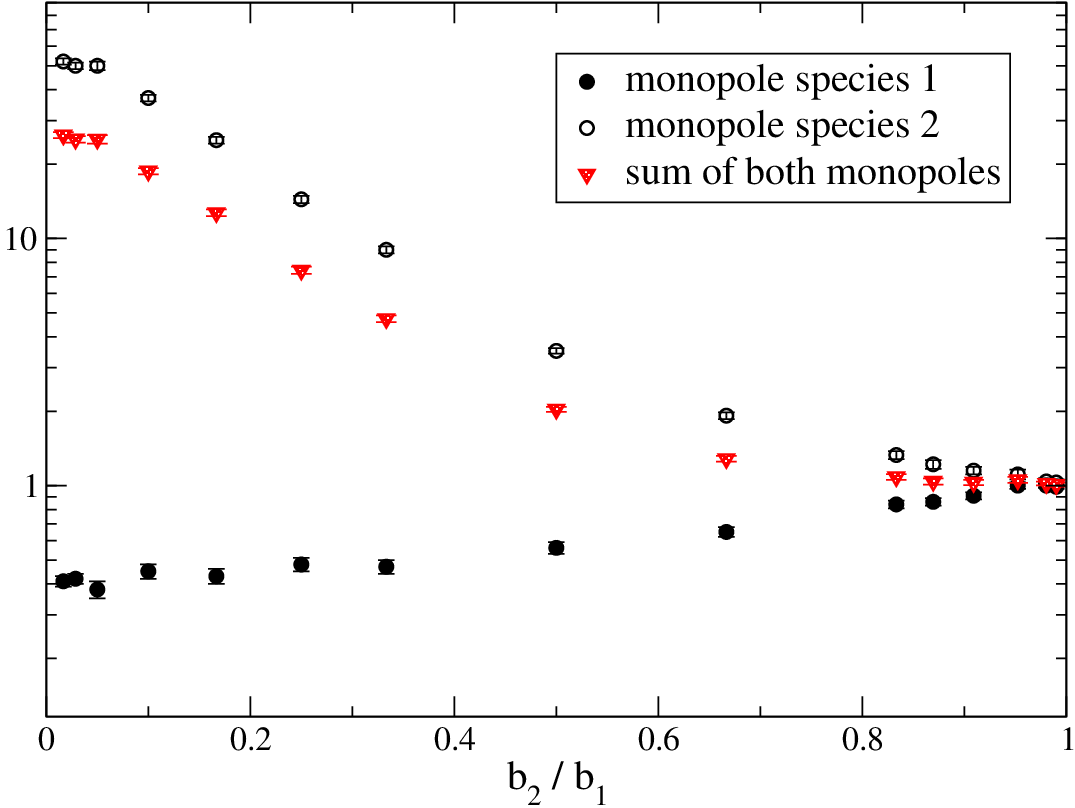
For that reason, in Fig. (11) we show the total density of 3D cubes containing monopole currents, separately for each monopole species, determined on a lattice at and as a function of (see Eq. (21)). Densities are normalized to that obtained at , which corresponds to our original choice. We report also the average of the two densities. Results show that, for small variations of around 1, the densities of the two species change but their sum remains stable. However, when , the density for species 2 grows by more than one order of magnitude: that can be related to the appearance of significant lattice artifacts in the identification of that kind of monopoles, due to the fact that , as discussed in Section II.3. Qualitatively similar results are obtained when one looks at thermal monopoles.
It is interesting to investigate which features remain stable when the ratio is modified. In Fig. (12) we report the analogous of Fig. (6), including chemical potentials obtained for the different monopole species and for . The effective chemical potentials show a clear dependence on . However, when one tries to fit data according to Eq. (35), to infer the temperature at which each monopole species shows signals of condensation, one finds , with , for monopole species 1, and , with , for monopole species 2. Hence, we infer that the temperature at which condensation seems to happen is stable under relatively small variations of . This is in nice agreement with the idea put forward in [31, 35] that the detection of monopoles is abelian-projection dependent but monopole condensation it is not.

References
- [1] G. ’t Hooft, in “High Energy Physics”, EPS International Conference, Palermo 1975, ed. A. Zichichi.
- [2] S. Mandelstam, Phys. Rept. 23, 245 (1976).
- [3] L. Del Debbio, A. Di Giacomo, G. Paffuti and P. Pieri, Phys. Lett. B 355, 255 (1995) [hep-lat/9505014].
- [4] A. Di Giacomo, B. Lucini, L. Montesi, G. Paffuti, Phys. Rev. D 61, 034503 (2000) [arXiv:hep-lat/9906024]; Phys. Rev. D 61, 034504 (2000) [arXiv:hep-lat/9906025];
- [5] J. M. Carmona, M. D’Elia, A. Di Giacomo, B. Lucini, G. Paffuti, Phys. Rev. D 64, 114507 (2001) [arXiv:hep-lat/0103005];
- [6] J. M. Carmona, M. D’Elia, L. Del Debbio, A. Di Giacomo, B. Lucini, G. Paffuti, Phys. Rev. D 66, 011503 (2002) [arXiv:hep-lat/0205025];
- [7] M. D’Elia, A. Di Giacomo, B. Lucini, G. Paffuti, C. Pica, Phys. Rev. D 71, 114502 (2005) [arXiv:hep-lat/0503035].
- [8] C. Bonati, G. Cossu, M. D’Elia and A. Di Giacomo, Phys. Rev. D 85, 065001 (2012) [arXiv:1111.1541 [hep-lat]].
- [9] M. N. Chernodub, M. I. Polikarpov and A. I. Veselov, Phys. Lett. B 399, 267 (1997).
- [10] P. Cea and L. Cosmai, JHEP 0111, 064 (2001); P. Cea, L. Cosmai and M. D’Elia, JHEP 0402, 018 (2004).
- [11] J. Liao, E. Shuryak, Phys. Rev. C 75 054907 (2007) [hep-ph/0611131].
- [12] M. N. Chernodub and V. I. Zakharov, Phys. Rev. Lett. 98, 082002 (2007) [arXiv:hep-ph/0611228]; M. N. Chernodub and V. I. Zakharov, arXiv:hep-ph/0702245.
- [13] V.G. Bornyakov, V.K. Mitrjushkin and M. Muller-Preussker Phys. Lett. B 284, 99 (1992).
- [14] S. Ejiri, Phys. Lett. B 376, 163 (1996) [arXiv:hep-lat/9510027].
- [15] A. D’Alessandro and M. D’Elia, Nucl. Phys. B 799, 241 (2008) [arXiv:0711.1266 [hep-lat]].
- [16] A. D’Alessandro, M. D’Elia and E. V. Shuryak, Phys. Rev. D 81, 094501 (2010) [arXiv:1002.4161 [hep-lat]].
- [17] M. N. Chernodub, A. D’Alessandro, M. D’Elia and V. I. Zakharov, arXiv:0909.5441 [hep-ph].
- [18] V. G. Bornyakov and V. V. Braguta, Phys. Rev. D 84, 074502 (2011) [arXiv:1104.1063 [hep-lat]].
- [19] V. G. Bornyakov and A. G. Kononenko, Phys. Rev. D 86, 074508 (2012) [arXiv:1111.0169 [hep-lat]].
- [20] V. G. Bornyakov and V. V. Braguta, Phys. Rev. D 85, 014502 (2012) [arXiv:1110.6308 [hep-lat]].
- [21] V. V. Braguta and A. Y. Kotov, Phys. Rev. D 86, 014511 (2012) [arXiv:1208.5344 [hep-lat]].
- [22] J. Liao and E. Shuryak, Phys. Rev. Lett. 101, 162302 (2008) [arXiv:0804.0255 [hep-ph]].
- [23] C. Ratti and E. Shuryak, Phys. Rev. D 80, 034004 (2009) [arXiv:0811.4174 [hep-ph]].
- [24] M. Cristoforetti and E. Shuryak, Phys. Rev. D 80, 054013 (2009) [arXiv:0906.2019 [hep-ph]].
- [25] V. G. Bornyakov, A. G. Kononenko and V. K. Mitrjushkin, PoS ConfinementX , 048 (2012).
- [26] G. ’t Hooft, Nucl. Phys. B 79, 276 (1974).
- [27] L. Del Debbio, A. Di Giacomo, B. Lucini and G. Paffuti, hep-lat/0203023.
- [28] A. Di Giacomo, L. Lepori and F. Pucci, JHEP 0810, 096 (2008) [arXiv:0810.4226 [hep-lat]].
- [29] G. ’t Hooft, Nucl. Phys. B 190, 455 (1981).
- [30] A. M. Polyakov, JETP Lett. 20, 194 (1974).
- [31] C. Bonati, A. Di Giacomo, L. Lepori and F. Pucci, Phys. Rev. D 81, 085022 (2010).
- [32] A. S. Kronfeld, G. Schierholz and U. J. Wiese, Nucl. Phys. B 293, 461 (1987).
- [33] A. De Grand, D. Toussaint, Phys. Rev. D 22 2478 (1980).
- [34] A. S. Kronfeld, M. L. Laursen, G. Schierholz, U.-J. Wiese Phys. Lett. B 198, 516 (1987).
- [35] C. Bonati, A. Di Giacomo and M. D’Elia, Phys. Rev. D 82, 094509 (2010) [arXiv:1009.2425 [hep-lat]].
- [36] F. Brandstaeter, G. Schierholz, U.-J. Wiese Phys. Lett. B 272, 319 (1991).
- [37] W. W. Tucker and J. D. Stack, Nucl. Phys. Proc. Suppl. 106, 643 (2002) [hep-lat/0110165].
- [38] V. Bornyakov, H. Ichie, S. Kitahara, Y. Koma, Y. Mori, Y. Nakamura, M. Polikarpov and G. Schierholz et al., Nucl. Phys. Proc. Suppl. 106, 634 (2002) [hep-lat/0111042].
- [39] V. G. Bornyakov et al. [DIK Collaboration], Phys. Rev. D 70, 054506 (2004) [hep-lat/0401026].
- [40] V. G. Bornyakov et al. [DIK Collaboration], Phys. Rev. D 70, 074511 (2004) [hep-lat/0310011].
- [41] J. D. Stack, W. W. Tucker, R. J. Wensley Nucl. Phys. B 639, 203 (2002) [hep-lat/0110196].
- [42] J. D. Stack, W. W. Tucker and R. J. Wensley, hep-lat/0205006.
- [43] W. W. Tucker and J. D. Stack, Nucl. Phys. Proc. Suppl. 119, 721 (2003) [hep-lat/0209134].
- [44] G. S. Bali, V. Bornyakov, M. Mueller-Preussker, K. Schilling, Phys. Rev. D 54 2863 (1996) [hep-lat/9603012]; V. G. Bornyakov, D. A. Komarov, M. I. Polikarpov, Phys. Lett. B 497 151 (2001).
- [45] C. Alexandrou, M. D’Elia and P. de Forcrand, Nucl. Phys. Proc. Suppl. 83, 437 (2000) [hep-lat/9907028].
- [46] P. de Forcrand and M. Pepe, Nucl. Phys. B 598, 557 (2001) [hep-lat/0008016].
- [47] N. Cabibbo and E. Marinari, Phys. Lett. B 119, 387 (1982).
- [48] M. Creutz, Phys. Rev. D 36, 515 (1987).
- [49] G. Boyd, J. Engels, F. Karsch, E. Laermann, C. Legeland, M. Lutgemeier and B. Petersson, Nucl. Phys. B 469, 419 (1996).
- [50] P. Giovannangeli and C. P. Korthals Altes, Nucl. Phys. B 608, 203 (2001) [arXiv:hep-ph/0102022].
- [51] R.P. Feynman, Phys. Rev. 90, 1116 (1953)
- [52] R.P. Feynman, Phys. Rev. 91, 1291 (1953)
- [53] V. Elser, PhD. Thesis, U.C. Berkeley, (1984)
- [54] M. Unsal and L. G. Yaffe, Phys. Rev. D 78, 065035 (2008) [arXiv:0803.0344 [hep-th]].
- [55] J. Liao and E. Shuryak, Phys. Rev. Lett. 109, 152001 (2012) [arXiv:1206.3989 [hep-ph]].
- [56] T. C. Kraan and P. van Baal, Phys. Lett. B 435, 389 (1998) [hep-th/9806034].
- [57] O. Bergman and G. Lifschytz, JHEP 0704, 043 (2007) [hep-th/0612289].
- [58] A. Parnachev and A. R. Zhitnitsky, Phys. Rev. D 78, 125002 (2008) [arXiv:0806.1736 [hep-ph]].
- [59] A. R. Zhitnitsky, Nucl. Phys. A 813, 279 (2008) [arXiv:0808.1447 [hep-ph]]; hep-ph/0601057.
- [60] C. Bonati, M. D’Elia, H. Panagopoulos and E. Vicari, Phys. Rev. Lett. 110, 252003 (2013) [arXiv:1301.7640 [hep-lat]].
- [61] M. D’Elia and F. Negro, arXiv:1306.2919 [hep-lat].
- [62] A. R. Zhitnitsky, arXiv:1308.0020 [hep-ph].
- [63] J. E. Mandula, M. Ogilvie Phys.Lett. B 248, 156 (1990).