跳到论文正文
W Papers独立论文阅读器 arXiv:1308.0224 论文正文 计算阅读时间 · 0%
引用这篇论文根据当前论文元数据生成,正式投稿前建议核对。


License: arXiv.org perpetual non-exclusive license
arXiv:1308.0224v3 [math.NA] 07 Dec 2015

Piecewise rigid curve deformation
via a Finsler steepest descent

Guillaume Charpiat Stars Lab INRIA Sophia-Antipolis Giacomo Nardi, Gabriel Peyré François-Xavier Vialard Ceremade, Université Paris-Dauphine Note: Guillaume.Charpiat@inria.fr Note: {nardi,peyre,vialard}@ceremade.dauphine.fr
Abstract

This paper introduces a novel steepest descent flow in Banach spaces. This extends previous works on generalized gradient descent, notably the work of Charpiat et al. [15], to the setting of Finsler metrics. Such a generalized gradient allows one to take into account a prior on deformations (e.g., piecewise rigid) in order to favor some specific evolutions. We define a Finsler gradient descent method to minimize a functional defined on a Banach space and we prove a convergence theorem for such a method. In particular, we show that the use of non-Hilbertian norms on Banach spaces is useful to study non-convex optimization problems where the geometry of the space might play a crucial role to avoid poor local minima. We show some applications to the curve matching problem. In particular, we characterize piecewise rigid deformations on the space of curves and we study several models to perform piecewise rigid evolution of curves.

2010 Mathematics Subject Classification: Primary 49M25; Secondary 65K10, 68U05.

Keywords: Curve evolution ; Finsler space ; gradient flow ; shape registration

1 Introduction

This paper introduces a new descent method to minimize energies defined over Banach spaces. This descent makes use of a generalized gradient which corresponds to a descent direction for a Finsler geometry. We show applications of this method to the optimization over the space of curves, where this Finsler gradient allows one to construct piecewise regular curve evolutions.

1.1 Previous Works

Energy minimization for curve evolution.

The main motivation for this work is the design of novel shape optimization methods, with an emphasis toward curves evolutions. Shape optimization is a central topic in computer vision, and has been introduced to solve various problems such as image segmentation or shape matching. These problems are often solved by introducing an energy which is minimized over the space of curves. The first variational method proposed to perform image segmentation through curve evolution is the snake model [25]. This initial proposal has been formalized using intrinsic energies depending only on the geometry of the curves. A first class of energies corresponds to a weighted length of the curve, where the weight acts as an edge detector [11, 28]. A second class of segmentation energies, pioneered by the Mumford-Shah model [31], integrates a penalization both inside and outside the curve, see for instance [12]. Shape registration requires to compute a matching between curves, which in turn can be solved by minimizing energies between pairs of curves. An elegant framework to design such energies uses distances over a space of measures or currents, see [21] for a detailed description and applications in medical imaging.

Curve evolution for image processing is an intense area of research, and we refer for instance to the following recent works for applications in image segmentation [32, 27, 23, 20] and matching [37, 46, 7].

Shape spaces as Riemannian spaces.

Minimizing these energies requires to define a suitable space of shapes and a notion of gradient with respect to the geometry of this space. The mathematical study of spaces of curves has been largely investigated in the last years, see for instance [50, 29]. The set of curves is naturally modeled over a Riemannian manifold [30]. This corresponds to using a Hilbertian metric on each tangent plane of the space of curves, i.e. the set of vector fields which deform infinitesimally a given curve. This Riemannian framework allows one to define geodesics which are shortest paths between two shapes [51, 22]. Computing minimizing geodesics is useful to perform shape registration [39, 45, 43], tracking [39] and shape deformation [26]. The theoretical study of the existence of these geodesics depends on the Riemannian metric. For instance, a striking result [30, 48, 49] is that the natural L2L^{2}-metric on the space of curves, that has been largely used in several applications in computer vision, is a degenerate Riemannian metric: any two curves have distance equal to zero with respect to such a metric.

Beside the computation of minimizing geodesics, Riemannian metrics are also useful to define descent directions for shape optimization. Several recent works [30, 14, 49, 48] point out that the choice of the metric, which the gradient depends on, notably affects the results of a gradient descent algorithm. Carefully designing the metric is thus crucial to reach better local minima of the energy. Modifying the descent flow can also be important for shape matching applications. A typical example of such Riemannian metrics are Sobolev-type metrics [40, 38, 42, 41] which lead to smooth curve evolutions.

Shape spaces as Finslerian spaces.

It is possible to extend the Riemannian framework by considering more general metrics on the tangent planes of the space of curves. Finsler spaces make use of Banach norms instead of Hilbertian norms [8]. A few recent works [29, 49] have studied the theoretical properties of Finslerian spaces of curves. To the best of our knowledge, with the notable exception of [15], which is discussed in detail in Section 1.4, no previous work has used Finslerian metrics for curve evolution.

Generalized gradient flow.

Beyond shape optimization, the use of non-Euclidean geometries is linked to the study of generalized gradient flows. Optimization on manifolds requires the use of Riemannian gradients and Riemannian Hessians, see for instance [1]. Second order schemes on manifolds can be used to accelerate shape optimization over Riemannian spaces of curves, see [34]. Optimization over Banach spaces requires the use of convex duality to define the associated gradient flow [24, 2, 5]. It is possible to generalize these flows for metric spaces using implicit descent steps, we refer to [4] for an overview of the theoretical properties of the resulting flows.

1.2 Motivation

The metrics defined over the tangent planes of the space of curves (e.g. an Hilbertian norm in the Riemannian case and a Banach norm in the Finsler case) have a major impact on the trajectory of the associated gradient descent. This choice thus allows one to favor specific evolutions. A first reason for introducing a problem-dependent metric is to enhance the performances of the optimization method. Energies minimized for shape optimization are non-convex, so a careful choice of the metric is helpful to avoid being trapped in a poor local minimum. A typical example is the curve registration problem, where reaching a non-global minimum makes the matching fail. A second reason is that, in some applications, one is actually interested in the whole descent trajectory, and not only in the local minimum computed by the algorithm. For the curve registration problem, the matching between the curves is obtained by tracking the bijection between the curves during the evolution. Taking into account desirable physical properties of the shapes, such as global or piecewise rigidity, is crucial to achieve state of the art results, see for instance [16, 13, 36]. In this article, we explore the use of Finsler gradient flows to encode piecewise rigid deformations of the curves.

1.3 Contributions

Our first contribution is the definition of a novel generalized gradient flow, that we call Finsler descent, and the study of the convergence properties of this flow. This Finsler gradient is obtained from the W1,2W^{1,2}-gradient through the resolution of a constrained convex optimization problem. Our second contribution is the instantiation of this general framework to define piecewise rigid curve evolutions, without knowing in advance the location of the articulations. This contribution includes the definition of novel Finsler penalties to encode piecewise rigid and piecewise similarity evolutions. It also includes the theoretical analysis of the convergence of the flow for B​V2BV^{2}-regular curves. Our last contribution is the application of these piecewise regular evolutions to the problem of curve registration. This includes the definition of a discretized flow using finite elements, and a comparison of the performances of Riemannian and Finsler flows for articulated shapes registration. The Matlab code to reproduce the numerical results of this article is available online11 1 https://www.ceremade.dauphine.fr/~peyre/codes/.

1.4 Relationship with [15]

Our work is partly inspired by the generalized gradient flow originally defined in [15]. We use a different formulation for our Finsler gradient, and in particular consider a convex constrained formulation, which allows us to prove convergence results. An application to piecewise rigid evolutions is also proposed in [15], but it differs significantly from our method. In [15], piecewise rigid flows are obtained using a non-convex penalty, which poses both theoretical difficulties (definition of a suitable functional space to make the descent method well-defined) and numerical difficulties (computation of descent direction as the global minimizer of a non-convex energy). In our work we prove a characterization of piecewise rigid deformations that enables the definition of a penalty depending on the deformation (instead of instantaneous parameters as done in [15]). Then, we generalize this penalty to the B​V2BV^{2}-framework obtaining a convex penalty for B​V2BV^{2}-piecewise rigid deformations.

1.5 Paper Organization

Section 2 defines the Finsler gradient and the associated steepest descent in Banach spaces, for which we prove a convergence theorem. Section 3 introduces the space of B​V2BV^{2}-curves and studies its main properties, in particular its stability to reparametrization. Section 4 characterizes C2C^{2}-piecewise rigid motions and defines a penalty in the case of B​V2BV^{2}-regular motions. We apply this method in Section 5 to the curve registration problem. We minimize a matching energy using the Finsler descent method for B​V2BV^{2}-piecewise rigid motions. Section 6 details the finite element discretization of the method. Section 7 gives numerical illustrations of the Finsler descent method for curve matching. Section 8 refines the model introduced in Section 4 to improve the matching results by replacing piecewise rigid transforms with piecewise similarities.

2 Finsler Descent Method in Banach Spaces

Let (H,⟨⋅,⋅⟩H)(H,\langle\cdot,\,\cdot\rangle_{H}) be a Hilbert space and let EE be a Fréchet differentiable energy defined on HH.

We consider a Banach space (ℬ,∥.∥ℬ)(\mathscr{B},\|.\|_{\mathscr{B}}) which is dense in HH and continuously embedded in HH, and we consider the restriction of EE to ℬ\mathscr{B} (such a restriction will be also denoted by EE).

We aim to solve the following minimization problem

infΓ∈ℬ​E​(Γ)\underset{\Gamma\in\mathscr{B}}{\inf}\;E(\Gamma) (2.1)

using a steepest descent method. We treat ℬ\mathscr{B} as a manifold modeled on itself and denote by TΓ​ℬT_{\Gamma}\mathscr{B} the tangent space at Γ∈ℬ\Gamma\in\mathscr{B}. In the following we suppose that at every point Γ∈ℬ\Gamma\in\mathscr{B}, the space TΓ​ℬT_{\Gamma}\mathscr{B} coincides with ℬ\mathscr{B}, although our descent method can be adapted to more general settings.

For every Γ∈ℬ\Gamma\in\mathscr{B} we define an inner product ⟨⋅,⋅⟩H⁡(Γ)\langle\cdot,\,\cdot\rangle_{H(\Gamma)} that is continuous with respect to Γ∈ℬ\Gamma\in\mathscr{B}, and we suppose that the norms ∥⋅∥H\|\cdot\|_{H} and ∥⋅∥H⁡(Γ)\|\cdot\|_{H(\Gamma)} are uniformly equivalent for every Γ\Gamma belonging to a ball of ℬ\mathscr{B} (with respect to the norm on ℬ\mathscr{B}). This makes HH complete with respect to the norm ∥⋅∥H⁡(Γ)\|\cdot\|_{H(\Gamma)}. Note that this inner product may be different from the inner product induced by ⟨⋅,⋅⟩H\langle\cdot,\,\cdot\rangle_{H} on TΓ​ℬT_{\Gamma}\mathscr{B}, and in particular it might depend on Γ\Gamma. For instance in the case of Sobolev metrics for the space of curves we usually consider H=W1,2​([0,1],ℝ2)H=W^{1,2}([0,1],\mathbb{R}^{2}) and set ℬ=TΓ​ℬ=W1,2​([0,1],ℝ2)\mathscr{B}=T_{\Gamma}\mathscr{B}=W^{1,2}([0,1],\mathbb{R}^{2}) equipped with the measure defined by the arclength of Γ\Gamma (see Remark 2.4).

Since EE is Fréchet differentiable and (H,⟨⋅,⋅⟩H⁡(Γ))(H,\langle\cdot,\,\cdot\rangle_{H(\Gamma)}) is a Hilbert space, by the Riesz representation theorem, there exists a unique vector v∈Hv\in H such that

D​E​(Γ)​(Φ)=⟨v,Φ⟩H⁡(Γ)∀Φ∈TΓ​ℬ.DE(\Gamma)(\Phi)=\langle v,\,\Phi\rangle_{H(\Gamma)}\quad\forall\,\Phi\in T_{\Gamma}\mathscr{B}\,.

The vector vv represents the gradient of EE at Γ\Gamma with respect to the inner product ⟨⋅,⋅⟩H⁡(Γ)\langle\cdot,\,\cdot\rangle_{H(\Gamma)}, and it is denoted by v=∇H⁡(Γ)E​(Γ)v=\nabla_{H(\Gamma)}E(\Gamma).

2.1 Finsler Gradient

The Finsler gradient determines a descent direction by modifying ∇H⁡(Γ)E​(Γ)\nabla_{H(\Gamma)}E(\Gamma) with respect to a penalty RΓR_{\Gamma} that depends on Γ\Gamma. It is defined by minimizing RΓR_{\Gamma} under a constraint ℒΓ\mathscr{L}_{\Gamma}.

Definition 2.1 (Finsler gradient).

For every Γ∈ℬ\Gamma\in\mathscr{B}, let RΓ:TΓ​ℬ→ℝ+∪{+∞}R_{\Gamma}:T_{\Gamma}\mathscr{B}\rightarrow{\mathbb{R}}^{+}\cup\{+\infty\} be a function such that RΓ≠+∞R_{\Gamma}\neq+\infty and ℒΓ⊂TΓ​ℬ\mathscr{L}_{\Gamma}\subset T_{\Gamma}\mathscr{B} a set satisfying

ℒΓ⊂{Φ∈TΓ​ℬ:⟨∇H⁡(Γ)E​(Γ),Φ⟩H⁡(Γ)⩾(1−ρ)​‖∇H⁡(Γ)E​(Γ)‖H⁡(Γ)​‖Φ‖H⁡(Γ)}\mathscr{L}_{\Gamma}\subset\left\{\Phi\in T_{\Gamma}\mathscr{B}\;:\;\left\langle\nabla_{H(\Gamma)}E(\Gamma),\Phi\right\rangle_{H(\Gamma)}\geqslant(1-\rho)\|\nabla_{H(\Gamma)}E(\Gamma)\|_{H(\Gamma)}\|\Phi\|_{H(\Gamma)}\right\}\, (2.2)

where ρ∈(0,1)\rho\in(0,1) is a fixed parameter independent of Γ\Gamma. This parameter is typically adapted to the targeted applications (see Section 7), and in particular to the energy EE. If RΓR_{\Gamma} admits a minimum on ℒΓ\mathscr{L}_{\Gamma} then a Finsler gradient for EE at Γ\Gamma with respect to RΓR_{\Gamma} is defined as:

∇RΓE​(Γ)∈argmin⁡{RΓ​(Φ):Φ∈ℒΓ}.\nabla_{R_{\Gamma}}E(\Gamma)\in{\rm argmin}\;\left\{R_{\Gamma}(\Phi)\;:\;\Phi\in\mathscr{L}_{\Gamma}\right\}\,. (2.3)

Note that if ∇H⁡(Γ)E​(Γ)=0\nabla_{H(\Gamma)}E(\Gamma)=0 then Γ\Gamma is a critical point and any descent algorithm stops. Note that RΓR_{\Gamma} is in general not equal to the Banach norm defined over the tangent space. This is important for some applications, such as the one considered in Section 4 (piecewise rigid deformations).

The next theorem gives an existence result for the Finsler gradient which is proved by using the standard direct method of calculus of variations.

Theorem 2.2.

Let TΓ​ℬT_{\Gamma}\mathscr{B} be a Banach space equipped with a topology 𝒯⁡(TΓ​ℬ)\mathscr{T}(T_{\Gamma}\mathscr{B}) such that every bounded sequence in TΓ​ℬT_{\Gamma}\mathscr{B} converges (up to a subsequence) with respect to the topology 𝒯⁡(TΓ​ℬ)\mathscr{T}(T_{\Gamma}\mathscr{B}). Let RΓR_{\Gamma} be coercive (i.e., RΓ​(Φ)→+∞R_{\Gamma}(\Phi)\rightarrow+\infty as ‖Φ‖TΓ​ℬ→+∞\|\Phi\|_{T_{\Gamma}\mathscr{B}}\rightarrow+\infty) and lower semi-continuous with respect to the topology 𝒯⁡(TΓ​ℬ)\mathscr{T}(T_{\Gamma}\mathscr{B}) and we suppose that ℒΓ\mathscr{L}_{\Gamma} is closed in TΓ​ℬT_{\Gamma}\mathscr{B} with respect to the topology 𝒯⁡(TΓ​ℬ)\mathscr{T}(T_{\Gamma}\mathscr{B}). Then Problem (2.3) admits at least a solution.

Proof.

As RΓR_{\Gamma} is coercive, every minimizing sequence is bounded in TΓ​ℬT_{\Gamma}\mathscr{B} so it converges (up to a subsequence) with respect to the topology 𝒯⁡(TΓ​ℬ)\mathscr{T}(T_{\Gamma}\mathscr{B}) toward an element of ℒΓ\mathscr{L}_{\Gamma}. Now, because of the lower semi-continuity of RΓR_{\Gamma}, the theorem ensues. ∎

Such a result is the generalization of the usual existence theorem of calculus of variations on a reflexive Banach space. In fact (see Corollary 3.23 p. 71 in [10]), if TΓ​ℬT_{\Gamma}\mathscr{B} is reflexive, the existence of the Finsler gradient is guaranteed whenever ℒΓ\mathscr{L}_{\Gamma} is convex and closed with respect to the strong topology of TΓ​ℬT_{\Gamma}\mathscr{B}, and RΓR_{\Gamma} is coercive, RΓ≠+∞R_{\Gamma}\neq+\infty, convex, and lower semi-continuous with respect to the strong topology of TΓ​ℬT_{\Gamma}\mathscr{B}. These hypotheses guarantee in particular an existence result if TΓ​ℬT_{\Gamma}\mathscr{B} is a Hilbert space.

The previous theorem guarantees the existence of a minimum on non-reflexive Banach spaces. The key point is the existence of a suitable topology which guarantees compactness of minimizing sequences. We point out that, in general, such a topology is weaker than the strong topology of the Banach space.

We point out that the applications studied in this work concern a minimization problem on TΓ​ℬ=B​V2​(𝕊1,ℝ2)T_{\Gamma}\mathscr{B}=BV^{2}(\mathbb{S}^{1},\mathbb{R}^{2}). Such a space is not reflexive but the weak* topology of B​V2​(𝕊1,ℝ2)BV^{2}(\mathbb{S}^{1},\mathbb{R}^{2}) satisfies the hypotheses of the previous theorem (see Appendix). Then, for some suitable set ℒΓ\mathscr{L}_{\Gamma} and penalty RΓR_{\Gamma}, the existence of the Finsler gradient is guaranteed.

The set ℒΓ\mathscr{L}_{\Gamma} imposes a constraint on the direction of the Finsler gradient and more precisely on the angle between the Finsler and Hilbert gradient. It is crucial to guarantee the convergence of the descent method by the Zoutendijk theorem (see Theorem 2.5). The parameter ρ\rho controls the deviation of the Finsler gradient with respect to ∇H⁡(Γ)E​(Γ)\nabla_{H(\Gamma)}E(\Gamma). This parameter can be tuned by the user to modify the geometry of the trajectory of the flow defined in Section 2.2. The impact of ρ\rho is studied by several numerical simulations in Section 7.1.

If the hypotheses of Theorem 2.2 are verified then the minimum in (2.3) exists, but in general it is not unique. A Finsler gradient is any minimum of the functional minimized in (2.3).

Condition (2.2) implies

⟨∇H⁡(Γ)E​(Γ)‖∇H⁡(Γ)E​(Γ)‖H⁡(Γ),∇RΓE​(Γ)‖∇RΓE​(Γ)‖H⁡(Γ)⟩H⁡(Γ)⩾(1−ρ)>0∀Γ∈ℬ.\left\langle\frac{\nabla_{H(\Gamma)}E(\Gamma)}{\|\nabla_{H(\Gamma)}E(\Gamma)\|_{H(\Gamma)}},\frac{\nabla_{R_{\Gamma}}E(\Gamma)}{\|\nabla_{R_{\Gamma}}E(\Gamma)\|_{H(\Gamma)}}\right\rangle_{H(\Gamma)}\geqslant(1-\rho)>0\quad\quad\forall\,\Gamma\in\mathscr{B}. (2.4)

This shows that the Finsler gradient is a valid descent direction, in the sense that

dd​t​E​(Γ−t​∇RΓE​(Γ))|t=0=−⟨∇H⁡(Γ)E​(Γ),∇RΓE​(Γ)⟩H⁡(Γ)< 0.\frac{\mathrm{d}}{\mathrm{d}t}E(\Gamma-t\nabla_{R_{\Gamma}}E(\Gamma))\Big|_{t=0}=-\langle\nabla_{H(\Gamma)}E(\Gamma),\,\nabla_{R_{\Gamma}}E(\Gamma)\rangle_{H(\Gamma)}<\,0\,.
Remark 2.3 (Relationship with [15]).

Our definition of Finsler gradient is partly inspired by the generalized gradient introduced in Section 6.1 of [15]. An important difference is that we introduce a constraint ℒΓ\mathscr{L}_{\Gamma} whereas  [15] defines the gradient as a minimum of D​E​(Γ)​(Φ)+RΓ​(Φ)DE(\Gamma)(\Phi)+R_{\Gamma}(\Phi) on TΓ​ℬT_{\Gamma}\mathscr{B}. This is a crucial point because, as shown in the next section, this constraint guarantees the convergence of the descent method associated with the Finsler gradient toward a stationary point of EE.

Remark 2.4 (Relationship with Sobolev gradient).

We consider the spaces ℬ=W1,2​([0,1],ℝ2)\mathscr{B}=W^{1,2}([0,1],\mathbb{R}^{2}), H=L2​([0,1],ℝ2)H=L^{2}([0,1],\mathbb{R}^{2}). More precisely, for every Γ∈ℬ\Gamma\in\mathscr{B}, we set TΓ​ℬ=W1,2​([0,1],ℝ2)T_{\Gamma}\mathscr{B}=W^{1,2}([0,1],\mathbb{R}^{2}) and we denote by L2​(Γ)L^{2}(\Gamma) the space L2​([0,1],ℝ2)L^{2}([0,1],\mathbb{R}^{2}) equipped with the norm

‖Ψ‖L2​(Γ)2=∫01|Ψ⁡(s)|2​|Γ′​(s)|​𝑑s.\|\Psi\|_{L^{2}(\Gamma)}^{2}=\int_{0}^{1}|\Psi(s)|^{2}|\Gamma^{\prime}(s)|\mathrm{d}s.

In order to make such a norm well-defined we suppose that |Γ′​(s)|≠0|\Gamma^{\prime}(s)|\neq 0 for a.e. s∈𝕊1s\in\mathbb{S}^{1}. This setting models smooth parametric planar curves and their deformations Ψ\Psi. Note that the space of curves is further detailed in Section 3.

We introduce

RΓ​(Φ)=‖D​Φ‖L2​(Γ)2,∀Φ∈TΓ​ℬ,R_{\Gamma}(\Phi)=\|D\Phi\|_{L^{2}(\Gamma)}^{2},\qquad\forall\,\Phi\in T_{\Gamma}\mathscr{B},
ℒΓ={Φ∈TΓ​ℬ:‖∇L2​(Γ)E​(Γ)−Φ‖L2​(Γ)⩽ρ​‖∇L2​(Γ)E​(Γ)‖L2​(Γ)}\mathscr{L}_{\Gamma}=\left\{\Phi\in T_{\Gamma}\mathscr{B}\;:\;\|\nabla_{L^{2}(\Gamma)}E(\Gamma)-\Phi\|_{L^{2}(\Gamma)}\leqslant\rho\|\nabla_{L^{2}(\Gamma)}E(\Gamma)\|_{L^{2}(\Gamma)}\right\}~ (2.5)

where we denote by D​ΦD\Phi the weak derivative of Φ\Phi. Note that ℒΓ\mathscr{L}_{\Gamma} satisfies condition (2.2). For a given differentiable energy EE, (2.3) becomes

∇RΓE​(Γ)∈argminΦ∈ℒΓ​‖D​Φ‖L2​(Γ)2.\nabla_{R_{\Gamma}}E(\Gamma)\in\underset{\Phi\in\mathscr{L}_{\Gamma}}{\argmin}\;\|D\Phi\|_{L^{2}(\Gamma)}^{2}~. (2.6)

We remark that, comparing with Proposition 4 p. 17 in [15], the Finsler gradient (2.6) represents a constrained version of the Sobolev gradient. Note also that in Definition 2.1, the penalty RΓR_{\Gamma} need not be quadratic so that the negative Finsler gradient can be understood as a generalization of the Sobolev gradient.

2.2 Finsler Descent Method

In this section we consider the minimization problem (2.1) of an energy EE on ℬ\mathscr{B}. Given some initialization Γ0∈ℬ\Gamma_{0}\in\mathscr{B}, the Finsler gradient descent is defined as

Γk+1=Γk−τk​∇RΓkE​(Γk)\Gamma_{k+1}=\Gamma_{k}-\tau_{k}\nabla_{R_{\Gamma_{k}}}E(\Gamma_{k}) (2.7)

where ∇RΓkE​(Γk)\nabla_{R_{\Gamma_{k}}}E(\Gamma_{k}) is any minimizer of (2.3) and the step size τ=τk>0\tau=\tau_{k}>0 is chosen in order to satisfy the Wolfe constraints

{E⁡(Γ+τ​v)⩽E⁡(Γ)+α​τ​⟨∇HE​(Γ),v⟩H⟨∇HE​(Γ+τ​v),v⟩H⩾β​⟨∇HE​(Γ),v⟩H\left\{\begin{array}[]{lll}E(\Gamma+\tau v)&\leqslant&E(\Gamma)+\alpha\tau\langle\nabla_{H}E(\Gamma),\,v\rangle_{H}\\ \langle\nabla_{H}E(\Gamma+\tau v),\,v\rangle_{H}&\geqslant&\beta\langle\nabla_{H}E(\Gamma),\,v\rangle_{H}\end{array}\right. (2.8)

for some fixed 0<α<β<10<\alpha<\beta<1 and with v=−∇RΓkE​(Γk)v=-\nabla_{R_{\Gamma_{k}}}E(\Gamma_{k}), see for instance [33], p.37.

We have the following result.

Theorem 2.5.

Let E∈C1​(H,ℝ+)E\in C^{1}(H,{\mathbb{R}}^{+}) be a non-negative energy. We suppose that there exists a constant L>0L>0 such that

‖∇HE​(Γ1)−∇HE​(Γ2)‖H⩽L​‖Γ1−Γ2‖H∀Γ1,Γ2∈H.\|\nabla_{H}E(\Gamma_{1})-\nabla_{H}E(\Gamma_{2})\|_{H}\leqslant L\|\Gamma_{1}-\Gamma_{2}\|_{H}\quad\forall\,\Gamma_{1},\Gamma_{2}\in H\,. (2.9)

Then, for the sequence {Γk}k\{\Gamma_{k}\}_{k} (defined in (2.7)), ‖∇HE​(Γk)‖H→0\|\nabla_{H}E(\Gamma_{k})\|_{H}\rightarrow 0.

Proof.

Since {Γk}\{\Gamma_{k}\} is the sequence defined by the gradient descent satisfying the assumption of the Zoutendijk theorem (see [33]: Theorem 3.2 p.43) for the ambient norm on HH, we have:

∑k=0∞⟨∇HE​(Γk)‖∇HE​(Γk)‖H,∇RΓkE​(Γk)‖∇RΓkE​(Γk)‖H⟩H2​‖∇HE​(Γk)‖H2<∞.\sum_{k=0}^{\infty}\langle\frac{\nabla_{H}E(\Gamma_{k})}{\|\nabla_{H}E(\Gamma_{k})\|_{H}},\,\frac{\nabla_{R_{\Gamma_{k}}}E(\Gamma_{k})}{\|\nabla_{R_{\Gamma_{k}}}E(\Gamma_{k})\|_{H}}\rangle_{H}^{2}\,\|\nabla_{H}E(\Gamma_{k})\|_{H}^{2}\,<\,\infty\,.

As we have assumed that the norms ∥⋅∥H\|\cdot\|_{H} and ∥⋅∥H⁡(Γ)\|\cdot\|_{H(\Gamma)} are equivalent on every bounded ball of ℬ\mathscr{B}, for kk large enough, the condition (2.4) implies :

⟨∇HE​(Γk)‖∇HE​(Γk)‖H,∇RΓkE​(Γk)‖∇RΓkE​(Γk)‖H⟩H⩾(1−ρ)​M>0\langle\frac{\nabla_{H}E(\Gamma_{k})}{\|\nabla_{H}E(\Gamma_{k})\|_{H}},\,\frac{\nabla_{R_{\Gamma_{k}}}E(\Gamma_{k})}{\|\nabla_{R_{\Gamma_{k}}}E(\Gamma_{k})\|_{H}}\rangle_{H}\geqslant(1-\rho)M>0\,

with M>0M>0. This follows by the fact that

⟨∇HE​(Γk),∇RΓkE⟩H=D​E​(Γk)​(∇RΓkE)=⟨∇H⁡(Γ)E​(Γk),∇RΓkE⟩H⁡(Γ)\langle\nabla_{H}E(\Gamma_{k}),\nabla_{R_{\Gamma_{k}}}E\rangle_{H}=DE(\Gamma_{k})(\nabla_{R_{\Gamma_{k}}}E)=\langle\nabla_{H(\Gamma)}E(\Gamma_{k}),\nabla_{R_{\Gamma_{k}}}E\rangle_{H(\Gamma)}

and the equivalence of the norms applied to (2.2).

Therefore, we have in particular

∑k=0∞‖∇HE​(Γk)‖H2<∞,\sum_{k=0}^{\infty}\,\|\nabla_{H}E(\Gamma_{k})\|_{H}^{2}\,<\,\infty\,,

and the result ensues. ∎

Remark 2.6 (On the Zoutendijk theorem).

In the previous proof we applied the Zoutendijk theorem in infinite dimensions which is not the case in  [33]. However, their proof can be straightforwardly generalized to the case of infinite dimensional Hilbert spaces.

Note that the sequence defined by the Finsler descent method could diverge (for instance if ∇HE​(Γ)→0\nabla_{H}E(\Gamma)\rightarrow 0 as ‖Γ‖ℬ→+∞\|\Gamma\|_{\mathscr{B}}\rightarrow+\infty). However, if EE is coercive, its level sets are compact with respect to some weaker topology τ\tau of ℬ\mathscr{B}, and the HH-gradient is continuous with respect to such a weak topology, then the previous theorem guarantees the convergence of the Finsler descent method toward a stationary point of the energy. In fact, as EE is coercive, we have that {Γk}\{\Gamma_{k}\} is uniformly bounded in ℬ\mathscr{B}. Then, as the level sets of EE are τ\tau-weakly compact, {Γk}\{\Gamma_{k}\} τ\tau-weakly converges (up to a subsequence) to an element of ℬ\mathscr{B}. Because of the continuity property of EE, such a point is a stationary point of EE.

Remark 2.7.

An interesting problem would be to show that the Finsler gradient descent scheme admits a limit flow when the step size tends to zero, or to show that the machinery of gradient flows over metric spaces (see [4]) can be adapted to our setting. We believe this is however not trivial and decided to leave this for future work.

3 Finsler Gradient in the Spaces of Curves

This section specializes our method to a space of piecewise-regular curves. We target applications to piecewise rigid evolutions to solve a curve matching problem (see Section 5). Note that, in order to perform piecewise rigid evolutions, we are led to deal with curves whose first and second derivatives are not continuous. This leads us to consider the setting of B​V2BV^{2}-functions. We refer the reader to Appendix for the definition and the main properties of B​VBV and B​V2BV^{2} functions.

3.1 B​V2BV^{2}-curves

In this section we define the space of B​V2BV^{2}-curves and introduce its main properties. This models closed, connected curves admitting a B​V2BV^{2}-parameterization.

In the following, for every Γ∈B​V2​(𝕊1,ℝ2)\Gamma\in BV^{2}(\mathbb{S}^{1},\mathbb{R}^{2}), we denote by d​Γ\mathrm{d}\Gamma the measure defined as

d​Γ​(A)=∫A|Γ′​(s)|​𝑑s,∀A⊂𝕊1\mathrm{d}\Gamma(A)=\int_{A}|\Gamma^{\prime}(s)|\mathrm{d}s\;,\quad\forall\,A\subset\mathbb{S}^{1}

where Γ′\Gamma^{\prime} denotes the approximate derivative of Γ\Gamma (see for instance [3]). In the following we identify [0,1][0,1] with the unit circle 𝕊1\mathbb{S}^{1}.

Definition 3.1 (B​V2BV^{2}-curves).

We set ℬ=B​V2​(𝕊1,ℝ2)\mathscr{B}=BV^{2}(\mathbb{S}^{1},{\mathbb{R}}^{2}) equipped with the B​V2BV^{2}-norm. For any Γ∈ℬ\Gamma\in\mathscr{B}, we set TΓ​ℬ=B​V2​(Γ)T_{\Gamma}\mathscr{B}=BV^{2}(\Gamma), the space B​V2​(𝕊1,ℝ2)BV^{2}(\mathbb{S}^{1},\mathbb{R}^{2}) equipped with the measure d​Γ\mathrm{d}\Gamma. In B​V2​(Γ)BV^{2}(\Gamma), differentiation and integration are done with respect to the measure d​Γ\mathrm{d}\Gamma. For every Φ∈TΓ​ℬ\Phi\in T_{\Gamma}\mathscr{B}, we have in particular

d​Φd​Γ​(s)=limε→0​Φ⁡(s+ε)−Φ⁡(s)d​Γ​((,,,)),‖Φ‖L1​(Γ)=∫𝕊1|Φ⁡(s)|​|Γ′​(s)|​𝑑s.\frac{\mathrm{d}\Phi}{\mathrm{d}\Gamma}(s)\,=\,\underset{\varepsilon\rightarrow 0}{\lim}\,\frac{\Phi(s+\varepsilon)-\Phi(s)}{\mathrm{d}\Gamma((s-\varepsilon,s+\varepsilon))}\,,\quad\|\Phi\|_{L^{1}(\Gamma)}=\int_{\mathbb{S}^{1}}|\Phi(s)||\Gamma^{\prime}(s)|\,\mathrm{d}s\,.

We also point out that d​Φd​Γ​(s)=Φ′​(s)/|Γ′​(s)|\frac{\mathrm{d}\Phi}{\mathrm{d}\Gamma}(s)=\Phi^{\prime}(s)/|\Gamma^{\prime}(s)| for a.e. s∈𝕊1s\in\mathbb{S}^{1}, which implies that such a derivative is Lebesgue-measurable. Remark that in order to make the previous derivation well defined we have to make a hypothesis on the derivative. We refer to next section, in particular to (3.10), for a discussion about the necessity of such a condition.

The first and second variation are defined as

TVΓ(Φ)=sup{∫𝕊1Φ(s)⋅d​gd​Γ(s)dΓ(s):g∈Cc1(𝕊1,ℝ2),∥g∥L∞​(𝕊1,ℝ2)⩽1}TV_{\Gamma}\left(\Phi\right)=\sup\left\{\int_{\mathbb{S}^{1}}\Phi(s)\cdot\frac{\mathrm{d}g}{\mathrm{d}\Gamma}(s)\,\mathrm{d}\Gamma(s)\;:\;g\in\mathrm{C}^{1}_{c}(\mathbb{S}^{1},\mathbb{R}^{2}),\|g\|_{L^{\infty}(\mathbb{S}^{1},{\mathbb{R}}^{2})}\leqslant 1\right\}\, (3.1)

and

TVΓ2(Φ)=sup{∫𝕊1Φ⋅d2​gd​Γ2(s)dΓ(s):g∈Cc2(𝕊1,ℝ2),∥g∥L∞​(𝕊1,ℝ2)⩽1}TV^{2}_{\Gamma}(\Phi)=\sup\left\{\int_{\mathbb{S}^{1}}\Phi\cdot\frac{\mathrm{d}^{2}g}{\mathrm{d}\Gamma^{2}}(s)\,\mathrm{d}\Gamma(s)\;:\;g\in\mathrm{C}^{2}_{c}({\mathbb{S}^{1}},\mathbb{R}^{2}),\|g\|_{L^{\infty}(\mathbb{S}^{1},\mathbb{R}^{2})}\leqslant 1\right\}\, (3.2)

for every Φ∈B​V2​(𝕊1,ℝ2)\Phi\in BV^{2}(\mathbb{S}^{1},\mathbb{R}^{2}). Now, as d​gd​Γ​(s)​d​Γ​(s)=g′​(s)​d​s\frac{\mathrm{d}g}{\mathrm{d}\Gamma}(s)\,\mathrm{d}\Gamma(s)=g^{\prime}(s)\,\mathrm{d}s we get T​VΓ​(Φ)=‖Φ′‖L1​(𝕊1,ℝ2)TV_{\Gamma}(\Phi)=\|\Phi^{\prime}\|_{L^{1}(\mathbb{S}^{1},\mathbb{R}^{2})}. The B​V2BV^{2}-norm on the tangent space is defined by

‖Φ‖B​V2​(Γ)=‖Φ‖W1,1​(Γ)+T​VΓ2​(Φ).\|\Phi\|_{BV^{2}(\Gamma)}=\|\Phi\|_{W^{1,1}(\Gamma)}+TV^{2}_{\Gamma}(\Phi)\,.

In a similar way we define W2,1​(Γ)W^{2,1}(\Gamma). Every Φ∈TΓ​ℬ\Phi\in T_{\Gamma}\mathscr{B} operates on a curve Γ∈ℬ\Gamma\in\mathscr{B} as

(Γ+Φ)​(s)=Γ⁡(s)+Φ⁡(s),∀s∈𝕊1.(\Gamma+\Phi)(s)=\Gamma(s)+\Phi(s)\,,\quad\forall\,s\in\mathbb{S}^{1}.
Definition 3.2 (Tangent, normal, and curvature).

For every Γ∈ℬ\Gamma\in\mathscr{B} we define the following vector

νΓ​(s)=limr→0​D​Γ​((,,,))|D​Γ|​((,,,))\nu_{\Gamma}(s)=\underset{r\rightarrow 0}{\lim}\,\frac{D\Gamma((s-r,s+r))}{|D\Gamma|((s-r,s+r))}\,

where |D​Γ||D\Gamma| denotes the total variation of Γ\Gamma and D​ΓD\Gamma denotes the vector-valued measure associated with the total variation. Note that, as Γ∈W1,1​(𝕊1,ℝ2)\Gamma\in W^{1,1}(\mathbb{S}^{1},\mathbb{R}^{2}), |D​Γ||D\Gamma| coincides with the measure d​Γ\mathrm{d}\Gamma (we recall that the total variation of a W1,1W^{1,1}-function coincides with the L1L^{1}-norm of its derivative) and the limit defining νΓ\nu_{\Gamma} exists for d​Γ\mathrm{d}\Gamma-a.e. s∈𝕊1s\in\mathbb{S}^{1}. Moreover we have ‖νΓ‖=1\|\nu_{\Gamma}\|=1 for d​Γ\mathrm{d}\Gamma-a.e. s∈𝕊1s\in\mathbb{S}^{1}.

Now, Γ∈W1,1​(𝕊1,ℝ2)\Gamma\in W^{1,1}(\mathbb{S}^{1},\mathbb{R}^{2}), and we can suppose that |Γ′​(s)|≠0|\Gamma^{\prime}(s)|\neq 0 for almost every s∈𝕊1s\in\mathbb{S}^{1}. This implies in particular that a subset of 𝕊1\mathbb{S}^{1} is d​Γ\mathrm{d}\Gamma-negligible if and only if it is Lebesgue-negligible. Then, the tangent and normal vectors to the curve at d​Γ\mathrm{d}\Gamma-a.e. point Γ⁡(s)\Gamma(s) are defined as

𝐭Γ​(s)=νΓ​(s)‖νΓ​(s)‖𝐧Γ​(s)=𝐭Γ​(s)⊥\mathbf{t}_{\Gamma}(s)=\frac{\nu_{\Gamma}(s)}{\|\nu_{\Gamma}(s)\|}\quad\quad\mathbf{n}_{\Gamma}(s)=\mathbf{t}_{\Gamma}(s)^{\bot} (3.3)
where(x,y)⊥=(−y,x),∀(x,y)∈ℝ2.\quad\text{where}\quad(x,y)^{\bot}=(-y,x)\;,\quad\forall\,(x,y)\in\mathbb{R}^{2}.

We point out that νΓ​(s)=Γ′​(s)/|Γ′​(s)|\nu_{\Gamma}(s)=\Gamma^{\prime}(s)/|\Gamma^{\prime}(s)| for a.e. s∈𝕊1s\in\mathbb{S}^{1} and 𝐭Γ∈B​V​(𝕊1,ℝ2)\mathbf{t}_{\Gamma}\in BV(\mathbb{S}^{1},\mathbb{R}^{2}) with 𝐭Γ⋅𝐭Γ=1\mathbf{t}_{\Gamma}\cdot\mathbf{t}_{\Gamma}=1 for a.e. s∈𝕊1s\in\mathbb{S}^{1}. Thus, by differentiating with respect to d​Γ\mathrm{d}\Gamma, we get that the measure 𝐭Γ⋅DΓ​𝐭Γ\mathbf{t}_{\Gamma}\cdot D_{\Gamma}\mathbf{t}_{\Gamma} is null (DΓD_{\Gamma} denotes here the vector-valued measure associated with the total variation T​VΓTV_{\Gamma}). Then, there exists a real measure curvΓ\rm{curv}_{\Gamma} such that

DΓ​𝐭Γ=𝐧Γ​curvΓ.D_{\Gamma}\mathbf{t}_{\Gamma}=\mathbf{n}_{\Gamma}\,\rm{curv}_{\Gamma}\,. (3.4)

By the definition of 𝐧Γ\mathbf{n}_{\Gamma} we also have

DΓ​𝐧Γ=−𝐭Γ​curvΓ.D_{\Gamma}\mathbf{n}_{\Gamma}=-\mathbf{t}_{\Gamma}\,\rm{curv}_{\Gamma}\,. (3.5)

The measure curvΓ\rm{curv}_{\Gamma} is called generalized curvature of Γ\Gamma, and, in the case of a smooth curve, it coincides with the measure κΓ​d​s\kappa_{\Gamma}\,\mathrm{d}s where κΓ\kappa_{\Gamma} denotes the standard scalar curvature of Γ\Gamma.

From the properties of the total variation (see for instance [3]) it follows that

|curvΓ|​(𝕊1)⩽|D2​Γ|​(𝕊1)|\rm{curv}_{\Gamma}|(\mathbb{S}^{1})\leqslant|D^{2}\Gamma|(\mathbb{S}^{1}) (3.6)

where |curvΓ|​(𝕊1)|\rm{curv}_{\Gamma}|(\mathbb{S}^{1}) denotes the total variation of the generalized curvature on the circle.

Definition 3.3 (Projectors).

We denote by ΠΓ\Pi_{\Gamma} the projection on the normal vector field 𝐧Γ\mathbf{n}_{\Gamma}

ΠΓ​(Φ)​(s)=(Φ⁡(s)⋅𝐧Γ​(s))​𝐧Γ​(s),\Pi_{\Gamma}(\Phi)(s)\;\;=\;\;\Big(\Phi(s)\cdot\mathbf{n}_{\Gamma}(s)\Big)\,\mathbf{n}_{\Gamma}(s), (3.7)

where ⋅\cdot is the inner product in ℝ2\mathbb{R}^{2}. We denote by ΣΓ\Sigma_{\Gamma} the projection on the tangent vector field 𝐭Γ\mathbf{t}_{\Gamma}

ΣΓ​(Φ)​(s)=(Φ⁡(s)⋅𝐭Γ​(s))​𝐭Γ​(s).\Sigma_{\Gamma}(\Phi)(s)\;\;=\;\;\Big(\Phi(s)\cdot\mathbf{t}_{\Gamma}(s)\Big)\,\mathbf{t}_{\Gamma}(s)\,. (3.8)
Definition 3.4 (Hilbertian structure).

The Banach space ℬ=B​V2​(𝕊1,ℝ2)\mathscr{B}=BV^{2}(\mathbb{S}^{1},\mathbb{R}^{2}) is continuously embedded in the Hilbert space H=W1,2​(𝕊1,ℝ2)H=W^{1,2}(\mathbb{S}^{1},\mathbb{R}^{2}).

For every Γ∈ℬ\Gamma\in\mathscr{B}, we define W1,2​(Γ)=W1,2​(𝕊1,ℝ2)W^{1,2}(\Gamma)=W^{1,2}(\mathbb{S}^{1},\mathbb{R}^{2}), where integration is done with respect to the measure d​Γ\mathrm{d}\Gamma. In particular, if Γ\Gamma verifies essinfs∈𝕊1​|Γ′​(s)|>0\underset{s\in\mathbb{S}^{1}}{{\rm essinf}}|\Gamma^{\prime}(s)|>0, then the norms of W1,2​(𝕊1,ℝ2)W^{1,2}(\mathbb{S}^{1},\mathbb{R}^{2}) and W1,2​(Γ)W^{1,2}(\Gamma) are equivalent. This defines the following inner product on TΓ​ℬT_{\Gamma}\mathscr{B}

⟨Φ,Ψ⟩W1,2​(Γ)=∫𝕊1Φ⁡(s)⋅Ψ⁡(s)​𝑑Γ​(s)+∫𝕊1d​Φd​Γ​(s)⋅d​Ψd​Γ​(s)​𝑑Γ​(s)∀Φ,Ψ∈TΓ​ℬ.\langle\Phi,\,\Psi\rangle_{W^{1,2}(\Gamma)}=\int_{\mathbb{S}^{1}}\Phi(s)\cdot\Psi(s)\;\mathrm{d}\Gamma(s)+\int_{\mathbb{S}^{1}}\frac{\mathrm{d}\Phi}{\mathrm{d}\Gamma}(s)\cdot\frac{\mathrm{d}\Psi}{\mathrm{d}\Gamma}(s)\;\mathrm{d}\Gamma(s)\quad\forall\,\Phi,\Psi\in T_{\Gamma}\mathscr{B}\,. (3.9)

Finally, recall that for a Fréchet-differentiable energy EE on HH, the W1,2​(Γ)W^{1,2}(\Gamma)-gradient of EE at Γ\Gamma is defined as the unique deformation ∇W1,2​(Γ)E​(Γ)\nabla_{W^{1,2}(\Gamma)}E(\Gamma) satisfying :

D​E​(Γ)​(Φ)=⟨∇W1,2​(Γ)E​(Γ),Φ⟩W1,2​(Γ),∀Φ∈TΓ​ℬDE(\Gamma)(\Phi)\;=\;\langle\nabla_{W^{1,2}(\Gamma)}E(\Gamma),\,\Phi\rangle_{W^{1,2}(\Gamma)}\,,\quad\forall\,\Phi\,\in\,T_{\Gamma}\mathscr{B}\,

where D​E​(Γ)​(Φ)DE(\Gamma)(\Phi) is the directional derivative.

3.2 Geometric Curves and Parameterizations

For applications in computer vision, it is important that the developed method (e.g. a gradient descent flow to minimize an energy) only depends on the actual geometry of the planar curve, and not on its particular parametrization. We denote [Γ]=Γ⁡(𝕊1)[\Gamma]=\Gamma(\mathbb{S}^{1}) the geometric realization of the curve, i.e. the image of the parameterization in the plane.

If, for two curves Γ1,Γ2∈ℬ\Gamma_{1},\Gamma_{2}\in\mathscr{B} there exists a smooth invertible map φ:𝕊1→𝕊1\varphi:\mathbb{S}^{1}\to\mathbb{S}^{1} such that Γ2=Γ1∘φ\Gamma_{2}=\Gamma_{1}\circ\varphi, then Γ2\Gamma_{2} is a reparameterization of Γ1\Gamma_{1} and these parameterizations share the same image, i.e. [Γ1]=[Γ2][\Gamma_{1}]=[\Gamma_{2}]. This section shows, in some sense, the converse implication in the B​V2BV^{2} framework, namely the existence of a reparameterization map between two curves sharing the same geometric realization. This result is important since it shows the geometric invariance of the developed Finsler gradient flow.

Note however that this is clearly not possible without any constraint on the considered curve. For instance, there is no canonical parameterization of an eight-shaped curve in the plane. We will only consider injective curves Γ∈ℬ\Gamma\in\mathscr{B} satisfying the following additional property

0∉Conv¯​(Γ′​(s+),Γ′​(s−))∀s∈𝕊1.0\notin\overline{\text{Conv}}(\Gamma^{\prime}(s^{+}),\Gamma^{\prime}(s^{-}))\quad\forall\,s\in\mathbb{S}^{1}\,. (3.10)

Here Conv¯\overline{\text{Conv}} denotes the closed convex envelope (a line segment) of the right and left limits Γ′​(s+)\Gamma^{\prime}(s^{+}) and OPENΓ′​(s−))\Gamma^{\prime}(s^{-})) of the derivative of Γ\Gamma at ss. We will show in the following that such a property gives a generalized definition of immersion for B​V2BV^{2}-curves and implies that the support of the curve has no cusp points.

We define the set of curves

ℬ0={Γ∈B​V2​(𝕊1,ℝ2):Γ​is injective and satisfies​(3.10)}\mathscr{B}_{0}=\{\Gamma\in BV^{2}(\mathbb{S}^{1},\mathbb{R}^{2})\,:\,\Gamma\;\mbox{is injective and satisfies}\;\eqref{cond-derivative}\} (3.11)

equipped with the B​V2BV^{2}-norm.

Note that it is difficult to ensure that the iterates {Γk}\{\Gamma_{k}\} defined by (2.7) stay in ℬ0\mathscr{B}_{0}, since ℬ0\mathscr{B}_{0} is not a linear space. As shown in Proposition 3.6 below, ℬ0\mathscr{B}_{0} is an open set, so that one might need to use small step sizes τk\tau_{k} to guarantee that Γk∈ℬ0\Gamma_{k}\in\mathscr{B}_{0}. This is however no acceptable, because it could contradict the constraints (2.8) and prevent the convergence of Γk\Gamma_{k} to a stationary point of EE. This issue reflects the well known fact that during an evolution, a parametric curve can cross itself and become non-injective.

We also note that, as pointed out in Definitions 3.4 and 3.1, condition (3.10) guarantees that the norms on L2​(𝕊1,ℝ2)L^{2}(\mathbb{S}^{1},\mathbb{R}^{2}) and L2​(Γ)L^{2}(\Gamma) and on B​V2​(𝕊1,ℝ2)BV^{2}(\mathbb{S}^{1},\mathbb{R}^{2}) and B​V2​(Γ)BV^{2}(\Gamma) are equivalent, so that the abstract setting described in Section 2 is adapted to our case.

We first show that property (3.10) implies local injectivity of the curve and that this local injectivity remains true in a neighborhood of the curve.

Proposition 3.5.

Let Γ0∈B​V2​(𝕊1,ℝ2)\Gamma_{0}\in BV^{2}(\mathbb{S}^{1},\mathbb{R}^{2}) and t∈𝕊1t\in\mathbb{S}^{1} such that condition (3.10) is satisfied. There exists ε>0,γ>0\varepsilon>0\,,\gamma>0 and n∈ℝ2n\in{\mathbb{R}}^{2} a unit vector such that, if ‖Γ0−Γ‖B​V2​(𝕊1,ℝ2)<γ\|\Gamma_{0}-\Gamma\|_{BV^{2}(\mathbb{S}^{1},\mathbb{R}^{2})}<\gamma, then Γ0\Gamma_{0} and Γ\Gamma are injective on |s−t|<ε|s-t|<\varepsilon, and

|⟨Γ⁡(s)−Γ⁡(t),n⟩|>γ​|s−t|on|s−t|<ε.|\langle\Gamma(s)-\Gamma(t),n\rangle|>\gamma|s-t|\quad\mbox{on}\quad|s-t|<\varepsilon\,.
Proof.

As Γ0′\Gamma_{0}^{\prime} is a function of bounded variation, the left and right limits exist and are finite. Moreover, Γ0\Gamma_{0} verifies (3.10) at tt if and only if there exists a unit vector nn such that ⟨Γ0′​(t+),n⟩>0\langle\Gamma_{0}^{\prime}(t^{+}),n\rangle>0 and ⟨Γ0′​(t−),n⟩>0\langle\Gamma_{0}^{\prime}(t^{-}),n\rangle>0. Let γ0=12​min⁡{⟨Γ0′​(t−),n⟩,⟨Γ0′​(t+),n⟩}\gamma_{0}=\frac{1}{2}\min\{\langle\Gamma_{0}^{\prime}(t^{-}),n\rangle,\langle\Gamma_{0}^{\prime}(t^{+}),n\rangle\}. By the fact that lims→t−Γ0′​(s)=Γ0′​(t−)\lim_{s\to t^{-}}\Gamma_{0}^{\prime}(s)=\Gamma_{0}^{\prime}(t^{-}) and lims→t+Γ0′​(s)=Γ0′​(t+)\lim_{s\to t^{+}}\Gamma_{0}^{\prime}(s)=\Gamma_{0}^{\prime}(t^{+}), there exists ε>0\varepsilon>0 such that

|⟨Γ0​(s)−Γ0​(t),n⟩|>γ0​|s−t|if|s−t|<ε,|\langle\Gamma_{0}(s)-\Gamma_{0}(t),n\rangle|>\gamma_{0}|s-t|\quad\mbox{if}\quad|s-t|<\varepsilon\,,

which proves the local injectivity for Γ0\Gamma_{0}.

Now, since B​V​(𝕊1,ℝ2)BV(\mathbb{S}^{1},\mathbb{R}^{2}) is continuously embedded in L∞​(𝕊1,ℝ2)L^{\infty}(\mathbb{S}^{1},\mathbb{R}^{2}), if ‖Γ0−Γ‖B​V2​(𝕊1,ℝ2)<γ0/2\|\Gamma_{0}-\Gamma\|_{BV^{2}(\mathbb{S}^{1},\mathbb{R}^{2})}<\gamma_{0}/2, then ⟨Γ′​(t+),n⟩>γ0/2\langle\Gamma^{\prime}(t^{+}),n\rangle>\gamma_{0}/2 and ⟨Γ′​(t−),n⟩>γ0/2\langle\Gamma^{\prime}(t^{-}),n\rangle>\gamma_{0}/2 which proves that Γ\Gamma verifies (3.10). Moreover we get

|⟨Γ⁡(s)−Γ⁡(t),n⟩|>γ02​|s−t|on|s−t|<ε,|\langle\Gamma(s)-\Gamma(t),n\rangle|>\frac{\gamma_{0}}{2}|s-t|\quad\mbox{on}\quad|s-t|<\varepsilon\,,

which proves the local injectivity of Γ\Gamma. The result ensues by setting γ=γ0/2\gamma=\gamma_{0}/2. ∎

Proposition 3.6.

ℬ0\mathscr{B}_{0} is an open set of ℬ=B​V2​(𝕊1,ℝ2)\mathscr{B}=BV^{2}(\mathbb{S}^{1},\mathbb{R}^{2}).

Proof.

If Λ∈ℬ0\Lambda\in\mathscr{B}_{0} then

m=essmins∈𝕊1​|Λ′​(s)|>0.m=\underset{s\in\mathbb{S}^{1}}{\rm{essmin}}\,|\Lambda^{\prime}(s)|>0\,.

Now, by Proposition 3.5, if

‖Γ−Λ‖B​V​(𝕊1,ℝ2)<m/4\|\Gamma-\Lambda\|_{BV(\mathbb{S}^{1},\mathbb{R}^{2})}<m/4

then Γ\Gamma is locally injective and verifies (3.10). Moreover, as 𝕊1\mathbb{S}^{1} is compact and (3.10) is satisfied on 𝕊1\mathbb{S}^{1}, there exists ε,α>0\varepsilon,\alpha>0 such that

|Λ⁡(s)−Λ⁡(s′)|⩾α​|s−s′|,∀s,s′∈𝕊1​such that​|s−s′|⩽ε.|\Lambda(s)-\Lambda(s^{\prime})|\geqslant\alpha|s-s^{\prime}|,\quad\forall\,s,s^{\prime}\in\mathbb{S}^{1}\;\;\mbox{such that}\;\;|s-s^{\prime}|\leqslant\varepsilon\,. (3.12)

Then, as Λ\Lambda is injective, if we take ‖Γ−Λ‖B​V2​(𝕊1,ℝ2)<β⁡(Λ)\|\Gamma-\Lambda\|_{BV^{2}(\mathbb{S}^{1},\mathbb{R}^{2})}<\beta(\Lambda) where

β⁡(Λ)=12​min​{α,infs∈𝕊1​inf|s−s′|>ε​‖Λ⁡(s)−Λ⁡(s′)‖}\beta(\Lambda)=\frac{1}{2}\mbox{min}\,\left\{\alpha,\underset{s\in\mathbb{S}^{1}}{\inf}\;\underset{|s-s^{\prime}|>\varepsilon}{\inf}\,\|\Lambda(s)-\Lambda(s^{\prime})\|\right\}

then Γ\Gamma is also globally injective.

Then

{Γ∈ℬ0|‖Γ−Λ‖B​V2​(𝕊1,ℝ2)<min⁡{m4,β⁡(Λ)}}⊂ℬ0\left\{\Gamma\in\mathscr{B}_{0}\,\big|\;\|\Gamma-\Lambda\|_{BV^{2}(\mathbb{S}^{1},\mathbb{R}^{2})}<{\rm{min}}\left\{\frac{m}{4},\beta(\Lambda)\right\}\right\}\subset\mathscr{B}_{0}\,

which proves that ℬ0\mathscr{B}_{0} is an open set of B​V2​(𝕊1,ℝ2)BV^{2}(\mathbb{S}^{1},\mathbb{R}^{2}). ∎

The next proposition proves the existence of a reparameterization between two curves sharing the same image.

Proposition 3.7.

(Reparameterization) For every Γ1,Γ2∈ℬ0\Gamma_{1},\Gamma_{2}\in\mathscr{B}_{0} such that [Γ1]=[Γ2][\Gamma_{1}]=[\Gamma_{2}], there exists a homeomorphism φ∈B​V2​(𝕊1,𝕊1)\varphi\in BV^{2}(\mathbb{S}^{1},\mathbb{S}^{1}) such that

Γ1=Γ2∘φ.\Gamma_{1}=\Gamma_{2}\circ\varphi\,.
Proof.

For every Γ1,Γ2∈ℬ0\Gamma_{1},\Gamma_{2}\in\mathscr{B}_{0} we consider the arc-length parameterizations defined by

φΓ1,φΓ2:𝕊1→𝕊1\varphi_{\Gamma_{1}},\varphi_{\Gamma_{2}}:\mathbb{S}^{1}\rightarrow\mathbb{S}^{1}
φΓ1​(s)=1Length​(Γ1)​∫s1s|Γ1′​(t)|​𝑑t,φΓ2​(s)=1Length​(Γ2)​∫s2s|Γ2′​(t)|​𝑑t\varphi_{\Gamma_{1}}(s)=\frac{1}{\mbox{Length}(\Gamma_{1})}\int_{s_{1}}^{s}\,|\Gamma_{1}^{\prime}(t)|\,dt\quad,\;\varphi_{\Gamma_{2}}(s)=\frac{1}{\mbox{Length}(\Gamma_{2})}\int_{s_{2}}^{s}\,|\Gamma_{2}^{\prime}(t)|\,dt

with s1,s2∈𝕊1s_{1},s_{2}\in\mathbb{S}^{1} such that Γ1​(s1)=Γ2​(s2)\Gamma_{1}(s_{1})=\Gamma_{2}(s_{2}).

Because of property (3.10) we can apply the inverse function theorem for Lipschitz functions (see Theorem 1 in [17]) which allows to define φΓ1−1,φΓ2−1∈B​V2​(𝕊1,𝕊1)\varphi_{\Gamma_{1}}^{-1},\varphi_{\Gamma_{2}}^{-1}\in BV^{2}(\mathbb{S}^{1},\mathbb{S}^{1}). It follows that

(Γ1∘φΓ1−1∘φΓ2)​(s)=Γ2​(s)∀s∈𝕊1.(\Gamma_{1}\circ\varphi_{\Gamma_{1}}^{-1}\circ\varphi_{\Gamma_{2}})(s)=\Gamma_{2}(s)\quad\forall\,s\in\mathbb{S}^{1}.

∎

3.3 Geometric Invariance

For B​V2BV^{2} curves, the geometric invariance of the developed methods should be understood as an invariance with respect to B​V2BV^{2} reparameterizations.

Definition 3.8.

Let GB​V2G_{BV^{2}} denote the set of homeomorphisms φ∈B​V2​(𝕊1,𝕊1)\varphi\in BV^{2}(\mathbb{S}^{1},\mathbb{S}^{1}) such that φ−1∈B​V2​(𝕊1,𝕊1)\varphi^{-1}\in BV^{2}(\mathbb{S}^{1},\mathbb{S}^{1}). Note that for every Γ∈B​V2​(𝕊1,ℝ2)\Gamma\in BV^{2}(\mathbb{S}^{1},\mathbb{R}^{2}) we have Γ∘φ∈B​V​(𝕊1,ℝ2)\Gamma\circ\varphi\in BV(\mathbb{S}^{1},\mathbb{R}^{2}) for every φ∈GB​V2\varphi\in G_{BV^{2}}. In fact, as every B​V2BV^{2}-function is Lipschitz-continuous, by the chain-rule for B​VBV-function, we get Γ∘φ∈B​V​(𝕊1,ℝ2)\Gamma\circ\varphi\in BV(\mathbb{S}^{1},\mathbb{R}^{2}). Moreover, (Γ∘φ)′=Γ′​(φ)​φ′∈B​V​(𝕊1,ℝ2)(\Gamma\circ\varphi)^{\prime}=\Gamma^{\prime}(\varphi)\varphi^{\prime}\in BV(\mathbb{S}^{1},\mathbb{R}^{2}) because B​VBV is a Banach algebra (one can check that Γ′​(φ)∈B​V​(𝕊1,ℝ2)\Gamma^{\prime}(\varphi)\in BV(\mathbb{S}^{1},\mathbb{R}^{2}) by performing the change of variables t=φ⁡(s)t=\varphi(s) in the definition of total variation).

To ensure this invariance, we consider energies EE and penalties RΓR_{\Gamma} such that

E⁡(Γ∘φ)=E⁡(Γ),RΓ∘φ​(Φ∘φ)=RΓ​(Φ)∀Γ∈ℬ0,∀φ∈GB​V2,∀Φ∈TΓ​ℬ.E(\Gamma\circ\varphi)=E(\Gamma)\;\;,\quad R_{\Gamma\circ\varphi}(\Phi\circ\varphi)=R_{\Gamma}(\Phi)\quad\quad\forall\,\Gamma\in\mathscr{B}_{0},\,\forall\,\varphi\in G_{BV^{2}},\,\forall\,\Phi\in T_{\Gamma}\mathscr{B}\,.

This implies that

∇RΓ∘φE​(Γ∘φ)​(Φ∘φ)=∇RΓE​(Γ)​(Φ)∘φ\nabla_{R_{\Gamma\circ\varphi}}E(\Gamma\circ\varphi)(\Phi\circ\varphi)=\nabla_{R_{\Gamma}}E(\Gamma)(\Phi)\circ\varphi

so that the descent scheme (2.7) does not depend on the parameterization of Γ\Gamma. Finally, as

(Γ−τ​∇RΓE​(Γ))∘φ=Γ∘φ−τ​∇RΓ∘φE​(Γ∘φ),(\Gamma-\tau\nabla_{R_{\Gamma}}E(\Gamma))\circ\varphi=\Gamma\circ\varphi-\tau\nabla_{R_{\Gamma\circ\varphi}}E(\Gamma\circ\varphi),

for τ=τk\tau=\tau_{k}, the descent step in (2.7) is also invariant under reparameterization.

This shows that the Finsler gradient flow can actually be defined over the quotient space ℬ/GB​V2\mathscr{B}/G_{BV^{2}}. To avoid unnecessary technicalities, we decided not to use this framework and develop our analysis in the setting of the vector space ℬ\mathscr{B}.

Another consequence of this invariance is that, as long as the evolution (2.7) is in ℬ0\mathscr{B}_{0}, the flow does not depend on the choice of the parameterization. However, as already noted in Section 3.2, it might happen that the sequence leaves ℬ0\mathscr{B}_{0}, in which case different choices of parameterizations of an initial geometric realization can lead to different evolutions.

4 Piecewise Rigidity

This section defines a penalty RΓR_{\Gamma} that favors piecewise rigid B​V2BV^{2} deformations of B​V2BV^{2}-curves. For the sake of clarity we present the construction of this penalty in two steps. We first characterize in Section 4.1 C2C^{2}-global rigid deformations for smooth curves. Then, in Section 4.2, we introduce a penalty that favors piecewise rigid B​V2BV^{2} deformations for curves belonging to ℬ\mathscr{B}.

4.1 Rigid Curve Deformations

A smooth curve evolution Γt∈C1​(ℝ,ℬ)\Gamma_{t}\in C^{1}(\mathbb{R},\mathscr{B}) reads

∀t∈ℝ,∂Γt​(s)∂t=Φt(s)whereΦt∈TΓ⁡(t)ℬ.\forall\,t\in\mathbb{R},\quad\frac{\partial\Gamma_{t}(s)}{\partial t}=\Phi_{t}(s)\quad\text{where}\quad\Phi_{t}\in T_{\Gamma(t)}\mathscr{B}\,. (4.1)

We further assume in this section that Γt\Gamma_{t} is a C2C^{2} curve. This evolution is said to be globally rigid if it preserves the pairwise distances between points along the curves, i.e.

∀t∈ℝ,∀(s,s′)∈𝕊1×𝕊1,|Γt​(s)−Γt​(s′)|=|Γ0​(s)−Γ0​(s′)|.\forall\,t\in\mathbb{R},\quad\forall\,(s,s^{\prime})\in\mathbb{S}^{1}\times\mathbb{S}^{1},\quad|\Gamma_{t}(s)-\Gamma_{t}(s^{\prime})|=|\Gamma_{0}(s)-\Gamma_{0}(s^{\prime})|. (4.2)

The following proposition shows that the set of instantaneous motions Φt\Phi_{t} giving rise to a rigid evolution is, at each time, a linear sub-space of dimension 3 of TΓt​ℬT_{\Gamma_{t}}\mathscr{B}.

Proposition 4.1.

The evolution (4.1) satisfies (4.2) if and only if Φt∈ℛΓt\Phi_{t}\in\mathscr{R}_{\Gamma_{t}} for all t∈ℝt\in\mathbb{R}, where

ℛΓ={Φ∈TΓℬ:∃a∈ℝ,∃b∈ℝ2,∀s∈𝕊1,Φ(s)=aΓ(s)⊥+b}.\mathscr{R}_{\Gamma}=\left\{\Phi\in T_{\Gamma}\mathscr{B}\;:\;\exists a\in\mathbb{R},\exists b\in{\mathbb{R}}^{2},\;\;\forall\,s\in\mathbb{S}^{1},\;\Phi(s)=a\,{\Gamma(s)}^{\bot}+b\right\}\,. (4.3)
Proof.

Recall that the group of distance preserving transformations on ℝd{\mathbb{R}}^{d} is the Euclidean group E⁡(d)=ℝd⋊Od​(ℝ)E(d)={\mathbb{R}}^{d}\rtimes O_{d}({\mathbb{R}}) and that any element of E⁡(d)E(d) is uniquely defined by the image of d+1d+1 points in ℝd{\mathbb{R}}^{d} which are affinely independent. Therefore, provided that the curve Γ\Gamma has at least three non-collinear points, Φt\Phi_{t} is the restriction of gt∈E⁡(d)g_{t}\in E(d), a path on E⁡(d)E(d) which is uniquely defined. In addition, gtg_{t} and Φt\Phi_{t} have the same smoothness. Thus the result follows from the fact that the Lie algebra of ℝd⋊Od​(ℝ){\mathbb{R}}^{d}\rtimes O_{d}({\mathbb{R}}) is ℝd⋊A⁡(d){\mathbb{R}}^{d}\rtimes A(d), where A⁡(d)A(d) denotes the set of antisymmetric matrices. The degenerate cases such as when the curve is contained in a line or a point are similar. ∎

Note that for numerical simulations, one replaces the continuous PDE (4.1) by a flow discretized at times tk=k​τt_{k}=k\tau for some step size τ>0\tau>0 and k∈ℕk\in\mathbb{N},

Γk+1=Γk+τ​ΦkwhereΦk∈TΓk​ℬ.\Gamma_{k+1}=\Gamma_{k}+\tau\Phi_{k}\quad\text{where}\quad\Phi_{k}\in T_{\Gamma_{k}}\mathscr{B}.

This is for instance the case of a gradient flow such as (2.7) where Φk=−∇RΓkE​(Γk)\Phi_{k}=-\nabla_{R_{\Gamma_{k}}}E(\Gamma_{k}). In this discretized setting, imposing Φk∈ℛΓk\Phi_{k}\in\mathscr{R}_{\Gamma_{k}} only guarantees that rigidity (4.2) holds approximately and for small enough times tkt_{k}.

The following proposition describes this set of tangent fields in an intrinsic manner (using only derivatives along the curve Γ\Gamma), and is pivotal to extend ℛΓ\mathscr{R}_{\Gamma} to piecewise-rigid tangent fields.

Proposition 4.2.

For a C2C^{2}-curve Γ\Gamma, one has Φ∈ℛΓ\Phi\in\mathscr{R}_{\Gamma} if and only if Φ\Phi is C2C^{2} and satisfies LΓ​(Φ)=0L_{\Gamma}(\Phi)=0 and HΓ​(Φ)=0H_{\Gamma}(\Phi)=0, where LΓL_{\Gamma} and HΓH_{\Gamma} are the following linear operators

LΓ​(Φ)=d​Φd​Γ⋅𝐭ΓandHΓ​(Φ)=d2​Φd​Γ2⋅𝐧Γ.L_{\Gamma}(\Phi)\;=\;\frac{\mathrm{d}\Phi}{\mathrm{d}\Gamma}\,\cdot\,\mathbf{t}_{\Gamma}\quad\text{and}\quad H_{\Gamma}(\Phi)\;=\;\frac{\mathrm{d}^{2}\Phi}{\mathrm{d}\Gamma^{2}}\,\cdot\,\mathbf{n}_{\Gamma}\,. (4.4)

From a geometric point of view, LΓ​(Φ)L_{\Gamma}(\Phi) takes into account the length changes and HΓ​(Φ)H_{\Gamma}(\Phi) the curvature changes.

Proof.

Using the parameterization of Γ\Gamma, any such deformation Φ\Phi satisfies

∃!(a,b)∈ℝ×ℝ2,∀s∈[0,1],Φ(s)=aΓ(s)⊥+b.\exists\,!\;(a,b)\in{\mathbb{R}}\times{\mathbb{R}}^{2},\quad\forall\,s\in[0,1],\quad\Phi(s)\;=\;a{\Gamma(s)}^{\bot}+b\,. (4.5)

By differentiation with respect to ​ ss, this is equivalent to

∃!a∈ℝ,∀s∈[0,1],d​Φd​s(s)=a|Γ′(s)|𝐧Γ(s)\exists\,!\;a\in{\mathbb{R}},\quad\forall\,s\in[0,1],\quad\frac{\mathrm{d}\Phi}{\mathrm{d}s}(s)\;=\;a|\Gamma^{\prime}(s)|\;\mathbf{n}_{\Gamma}(s)

which can be rewritten as d​Φd​Γ​(s)=a​𝐧Γ​(s)\frac{\mathrm{d}\Phi}{\mathrm{d}\Gamma}(s)=a\mathbf{n}_{\Gamma}(s) by differentiating with respect to ​ the length element d​Γ=‖Γ′​(s)‖​d​s\mathrm{d}\Gamma=\|\Gamma^{\prime}(s)\|\,\mathrm{d}s, or simply as d​Φd​s​(s)=a​𝐧Γ​(s)\frac{\mathrm{d}\Phi}{\mathrm{d}s}(s)=a\mathbf{n}_{\Gamma}(s) by considering an arc-length parameterization. This is equivalent to

∃!a∈ℝ,∀s∈[0,1],{d​Φd​Γ⋅𝐭Γ​(s)= 0d​Φd​Γ⋅𝐧Γ​(s)=a\exists\,!\;a\in{\mathbb{R}},\quad\forall\,s\in[0,1],\quad\begin{cases}\displaystyle\;\;\frac{\mathrm{d}\Phi}{\mathrm{d}\Gamma}\,\cdot\,\mathbf{t}_{\Gamma}(s)\;=\;0\vskip 5.69054pt\\ \displaystyle\;\;\frac{\mathrm{d}\Phi}{\mathrm{d}\Gamma}\,\cdot\,\mathbf{n}_{\Gamma}(s)\;=\;a\end{cases}

which is equivalent to

{d​Φd​Γ⋅𝐭Γ= 0dd​Γ​(d​Φd​Γ⋅𝐧Γ)= 0\begin{cases}\displaystyle\;\;\frac{\mathrm{d}\Phi}{\mathrm{d}\Gamma}\,\cdot\,\mathbf{t}_{\Gamma}\;=\;0\vskip 5.69054pt\\ \displaystyle\;\;\frac{\mathrm{d}}{\mathrm{d}\Gamma}\left(\frac{\mathrm{d}\Phi}{\mathrm{d}\Gamma}\,\cdot\,\mathbf{n}_{\Gamma}\right)\;=\;0\end{cases}

and, using that

dd​Γ​(d​Φd​Γ⋅𝐧Γ)=d2​Φd​Γ2⋅𝐧Γ−d​Φd​Γ⋅κΓ​𝐭Γ,\frac{\mathrm{d}}{\mathrm{d}\Gamma}\left(\frac{\mathrm{d}\Phi}{\mathrm{d}\Gamma}\,\cdot\,\mathbf{n}_{\Gamma}\right)\;=\;\frac{\mathrm{d}^{2}\Phi}{\mathrm{d}\Gamma^{2}}\,\cdot\,\mathbf{n}_{\Gamma}\;-\frac{\mathrm{d}\Phi}{\mathrm{d}\Gamma}\,\cdot\,\kappa_{\Gamma}\,\mathbf{t}_{\Gamma},

where κΓ\kappa_{\Gamma} is the curvature of Γ\Gamma, we obtain the desired characterization. ∎

4.2 Piecewise rigid B​V2BV^{2} deformations

This section extends the globally rigid evolution considered in the previous section to piecewise-rigid evolution.

In the smooth case considered in the previous section, this corresponds to imposing that an instantaneous deformation Φ∈TΓ​ℬ\Phi\in T_{\Gamma}\mathscr{B} satisfies (4.4) piecewisely for possibly different pairs (a,b)(a,b) on each piece. To generate a piecewise-smooth Finsler gradient Φ=∇RΓE​(Γ)\Phi=\nabla_{R_{\Gamma}}E(\Gamma) (as defined in (2.3)) that is a piecewise rigid deformation, one should design a penalty RΓR_{\Gamma} that satisfies this property. This is equivalent to imposing LΓ​(Φ)=0L_{\Gamma}(\Phi)=0 and HΓ​(Φ)=0H_{\Gamma}(\Phi)=0 for all s∈[0,1]s\in[0,1] except for a finite number of points (the articulations between the pieces). In particular, note that LΓ​(Φ)L_{\Gamma}(\Phi) is undefined at these points, while HΓ​(Φ)H_{\Gamma}(\Phi) is the sum of Dirac measures concentrated at the articulation points (due to the variations of aa). This suggests that, in the smooth case, we can favor piecewise rigidity by minimizing ‖HΓ​(Φ)‖L1​(Γ)\left\|H_{\Gamma}(\Phi)\right\|_{L^{1}(\Gamma)} under the constraint LΓ​(Φ)=0​a.e.L_{\Gamma}(\Phi)=0\;\;a.e., so that we control the jumps of the second derivative without setting in advance the articulation points. Note also that the minimization of the L1L^{1}-norm favors sparsity and, in contrast to the L2L^{2}-norm, it enables the emergence of Dirac measures.

In order to extend such an idea to the B​V2BV^{2}-framework we remind that

‖HΓ​(Φ)‖L1​(Γ)=T​VΓ​(d​Φd​Γ⋅𝐧Γ)∀Φ∈C2​(𝕊1,ℝ2),Γ∈C2​(𝕊1,ℝ2)\left\|H_{\Gamma}(\Phi)\right\|_{L^{1}(\Gamma)}=TV_{\Gamma}\left(\frac{\mathrm{d}\Phi}{\mathrm{d}\Gamma}\cdot\mathbf{n}_{\Gamma}\right)\quad\forall\,\Phi\in C^{2}(\mathbb{S}^{1},\mathbb{R}^{2}),\,\Gamma\in C^{2}(\mathbb{S}^{1},\mathbb{R}^{2})

which defines a suitable penalty in the B​V2BV^{2}-setting. Moreover, since we are interested in piecewise rigid motions, we deal with curves that could be not C1C^{1} at some points ss. It is useful to introduce the following operators

LΓ+​(Φ)​(s)\displaystyle L_{\Gamma}^{+}(\Phi)(s) =limt→st∈(s,s+ε)​d​Φd​Γ​(t)⋅𝐭Γ​(t),\displaystyle=\underset{\underset{t\in(s,s+\varepsilon)}{t\rightarrow s}}{\lim}\frac{\mathrm{d}\Phi}{\mathrm{d}\Gamma}(t)\cdot\,\mathbf{t}_{\Gamma}(t)\,, (4.6)
LΓ−​(Φ)​(s)\displaystyle L_{\Gamma}^{-}(\Phi)(s) =limt→st∈(s−ε,s)​d​Φd​Γ​(t)⋅𝐭Γ​(t).\displaystyle=\underset{\underset{t\in(s-\varepsilon,s)}{t\rightarrow s}}{\lim}\frac{\mathrm{d}\Phi}{\mathrm{d}\Gamma}(t)\cdot\,\mathbf{t}_{\Gamma}(t)\,. (4.7)

Of course if Γ\Gamma and Φ\Phi are C1C^{1} at ss we have LΓ+​(Φ)​(s)=LΓ−​(Φ)​(s)=LΓ​(Φ)​(s)L_{\Gamma}^{+}(\Phi)(s)=L_{\Gamma}^{-}(\Phi)(s)=L_{\Gamma}(\Phi)(s). The next definition introduces a penalty for piecewise rigid evolution in ℬ\mathscr{B}.

Definition 4.3 (B​V2BV^{2} Piecewise-rigid penalty).

For Γ∈ℬ\Gamma\in\mathscr{B} and Φ∈TΓ​ℬ=B​V2​(Γ)\Phi\in T_{\Gamma}\mathscr{B}=BV^{2}(\Gamma), we define

RΓ​(Φ)=T​VΓ​(d​Φd​Γ⋅𝐧Γ)+ι𝒞Γ​(Φ)R_{\Gamma}(\Phi)=TV_{\Gamma}\left(\frac{\mathrm{d}\Phi}{\mathrm{d}\Gamma}\cdot\mathbf{n}_{\Gamma}\right)+\iota_{\mathscr{C}_{\Gamma}}(\Phi) (4.8)

where ι𝒞Γ\iota_{\mathscr{C}_{\Gamma}} is the indicator function of 𝒞Γ\mathscr{C}_{\Gamma}

ι𝒞Γ​(Φ)={0if ​Φ∈𝒞Γ+∞otherwise .\displaystyle{\iota_{\mathscr{C}_{\Gamma}}(\Phi)=\left\{\begin{array}[]{ll}0&\text{if }\Phi\in\mathscr{C}_{\Gamma}\\ +\infty&\text{otherwise }\end{array}\right.}\,.

Note that (3.1) is the total variation of ff with respect to the measure d​Γ\mathrm{d}\Gamma. We remind that T​VΓ​(f)=|D​f|(𝕊1)TV_{\Gamma}(f)=|Df|(\mathbb{S}^{1}) for every f∈L1​(𝕊1,ℝ2)f\in L^{1}(\mathbb{S}^{1},\mathbb{R}^{2}).

The set 𝒞Γ\mathscr{C}_{\Gamma} is defined as follows

𝒞Γ={Φ∈TΓ​ℬ:LΓ+​(Φ)=LΓ−​(Φ)=0}.\mathscr{C}_{\Gamma}=\left\{\Phi\in T_{\Gamma}\mathscr{B}\;:\;L^{+}_{\Gamma}(\Phi)=L^{-}_{\Gamma}(\Phi)=0\right\}\,. (4.9)

In order to define the Finsler gradient we consider a constraint on the normal component of the deformation field.

Definition 4.4 (Deviation constraint).

For Γ∈ℬ\Gamma\in\mathscr{B}, we define

ℒΓ={Φ∈TΓ​ℬ:‖ΠΓ​(∇W1,2​(Γ)E​(Γ)−Φ)‖W1,2​(Γ)⩽ρ​‖ΠΓ​(∇W1,2​(Γ)E​(Γ))‖W1,2​(Γ)}.\mathscr{L}_{\Gamma}=\left\{\Phi\in T_{\Gamma}\mathscr{B}\;:\;\big\|\Pi_{\Gamma}(\nabla_{\!W^{1,2}(\Gamma)}E(\Gamma)-\Phi)\big\|_{W^{1,2}(\Gamma)}\leqslant\rho\big\|\Pi_{\Gamma}(\nabla_{\!W^{1,2}(\Gamma)}E(\Gamma))\big\|_{W^{1,2}(\Gamma)}\right\}\,. (4.10)

Here, ρ∈(0,1)\rho\in(0,1) is called the rigidification parameter, and controls the deviation of the Finsler gradient from the W1,2W^{1,2} gradient. ΠΓ\Pi_{\Gamma} is the projector introduced in equation (3.7).

We point out that in the applications studied in this paper we consider an intrinsic energy EE (i.e., it does not depend on reparameterization). In this case the W1,2W^{1,2}-gradient of EE is normal to the curve, so that ℒΓ\mathscr{L}_{\Gamma} satisfies condition (2.2) in the case of an intrinsic energy, and it can be used to define a valid Finsler gradient.

Using these specific instantiations for RΓR_{\Gamma} and ℒΓ\mathscr{L}_{\Gamma}, Definition 2.1 reads in this B​V2BV^{2} framework as follows.

Definition 4.5 (B​V2BV^{2} Piecewise-rigid Finsler gradient).

We define

∇RΓE​(Γ)∈argminΦ∈ℒΓ​RΓ​(Φ).\nabla_{R_{\Gamma}}E(\Gamma)\in\underset{\Phi\in\mathscr{L}_{\Gamma}}{\argmin}\;\;R_{\Gamma}(\Phi). (4.11)

The following result ensures the existence of a Finsler gradient. To prove it we consider the space ℬ\mathscr{B} equipped with the weak* toplogy.

Theorem 4.6.

Problem (4.11) admits at least a solution.

In order to prove the theorem, we need the following lemmas. They guarantee in particular the compactness of minimizing sequences with respect to the B​V2BV^{2}-weak* topology. The proof relies on the evaluation of a bilinear form which is degenerate if the curve is a circle, so we treat the case of the circle separately.

Lemma 4.7.

Let Γ∈ℬ\Gamma\in\mathscr{B} be an injective curve. We suppose that Γ\Gamma is different from a circle. Then there exists a constant C⁡(Γ)C(\Gamma) depending on Γ\Gamma such that

‖Φ‖B​V2​(Γ)⩽C⁡(Γ)​((1+ρ)​‖ΠΓ​(∇W1,2​(Γ)E​(Γ))‖W1,2​(Γ)+RΓ​(Φ))∀Φ∈ℒΓ∩𝒞Γ\|\Phi\|_{BV^{2}(\Gamma)}\leqslant C(\Gamma)\left((1+\rho)\|\Pi_{\Gamma}(\nabla_{W^{1,2}(\Gamma)}E(\Gamma))\|_{W^{1,2}(\Gamma)}+R_{\Gamma}(\Phi)\right)\quad\forall\,\Phi\in\mathscr{L}_{\Gamma}\cap\mathscr{C}_{\Gamma} (4.12)

where ΠΓ\Pi_{\Gamma} is the operator defined in (3.7).

Proof.

The proof is essentially based on estimation (4.14) giving a bound for the L∞L^{\infty}-norms of the deformation Φ\Phi and its first derivative. We also remark that, as Φ∈ℒΓ\Phi\in\mathscr{L}_{\Gamma}, we have

‖ΠΓ​(Φ)‖L2​(Γ)⩽(1+ρ)​‖ΠΓ​(∇W1,2​(Γ)E​(Γ))‖W1,2​(Γ).\|\Pi_{\Gamma}(\Phi)\|_{L^{2}(\Gamma)}\leqslant(1+\rho)\|\Pi_{\Gamma}(\nabla_{W^{1,2}(\Gamma)}E(\Gamma))\|_{W^{1,2}(\Gamma)}\,. (4.13)

In the following we denote by l⁡(Γ)l(\Gamma) the length of the curve Γ\Gamma.

Bound on the first derivative. In this section we prove the following estimate for the L∞L^{\infty}-norms of d​Φd​Γ⋅𝐧Γ\frac{\mathrm{d}\Phi}{\mathrm{d}\Gamma}\cdot\mathbf{n}_{\Gamma} and Φ\Phi:

max​{‖Φ‖L∞​(Γ);‖d​Φd​Γ⋅𝐧Γ‖L∞​(Γ)}⩽C0​(Γ)​((1+ρ)​‖ΠΓ​(∇W1,2​(Γ)E​(Γ))‖W1,2​(Γ)+RΓ​(Φ))\mbox{max}\left\{\left\|\Phi\right\|_{L^{\infty}(\Gamma)}\,;\,\left\|\frac{\mathrm{d}\Phi}{\mathrm{d}\Gamma}\cdot\mathbf{n}_{\Gamma}\right\|_{L^{\infty}(\Gamma)}\right\}\leqslant C_{0}(\Gamma)\left((1+\rho)\|\Pi_{\Gamma}(\nabla_{W^{1,2}(\Gamma)}E(\Gamma))\|_{W^{1,2}(\Gamma)}+R_{\Gamma}(\Phi)\right)\, (4.14)

where C0​(Γ)C_{0}(\Gamma) depends on Γ\Gamma.

Let s0∈𝕊1s_{0}\in\mathbb{S}^{1}, we can write

d​Φd​Γ⋅𝐧Γ=u+a\frac{\mathrm{d}\Phi}{\mathrm{d}\Gamma}\cdot\mathbf{n}_{\Gamma}=u+a

where u∈B​V​(Γ)u\in BV(\Gamma) such that u⁡(s0)=0u(s_{0})=0 and a=d​Φd​Γ​(s0)⋅𝐧Γ​(s0)∈ℝa=\frac{\mathrm{d}\Phi}{\mathrm{d}\Gamma}(s_{0})\cdot\mathbf{n}_{\Gamma}(s_{0})\in{\mathbb{R}}. As Φ∈𝒞Γ\Phi\in\mathscr{C}_{\Gamma} we have LΓ+​(Φ)=LΓ−​(Φ)=0L_{\Gamma}^{+}(\Phi)=L_{\Gamma}^{-}(\Phi)=0, which implies

d​Φd​Γ=(d​Φd​Γ⋅𝐧Γ)​𝐧Γ\frac{\mathrm{d}\Phi}{\mathrm{d}\Gamma}=\left(\frac{\mathrm{d}\Phi}{\mathrm{d}\Gamma}\cdot\mathbf{n}_{\Gamma}\right)\mathbf{n}_{\Gamma}

and

Φ⁡(s)=Φ⁡(s0)+a​[Γ⁡(s)−Γ⁡(s0)]⊥+∫s0su​𝐧Γ​𝑑Γ​(s)∀s∈𝕊1.\Phi(s)=\Phi(s_{0})+a[\Gamma(s)-\Gamma(s_{0})]^{\bot}+\int_{s_{0}}^{s}u\mathbf{n}_{\Gamma}\mathrm{d}\Gamma(s)\,\quad\forall\,s\in\mathbb{S}^{1}\,. (4.15)

Now, by projecting on the normal to Γ\Gamma, we can write

ΠΓ​(Φ)=ΠΓ​(Φ⁡(s0)+a​[Γ⁡(s)−Γ⁡(s0)]⊥)+ΠΓ​(∫s0su​𝐧Γ​𝑑Γ​(s)).\Pi_{\Gamma}(\Phi)=\Pi_{\Gamma}(\Phi(s_{0})+a[\Gamma(s)-\Gamma(s_{0})]^{\bot})+\Pi_{\Gamma}\left(\int_{s_{0}}^{s}u\mathbf{n}_{\Gamma}\mathrm{d}\Gamma(s)\right)\,. (4.16)

In particular, by the properties of good representatives for B​VBV-functions of one variable (see [3] p. 19), we have

|u⁡(s)|=|u⁡(s)−u⁡(s0)|⩽T​VΓ​(u)∀s∈𝕊1|u(s)|=|u(s)-u(s_{0})|\leqslant TV_{\Gamma}(u)\quad\forall s\in\mathbb{S}^{1}

which implies that

‖∫s0su​𝐧Γ​𝑑Γ​(s)‖L∞​(Γ)⩽l⁡(Γ)​T​VΓ​(u)=l⁡(Γ)​RΓ​(Φ)\left\|\int_{s_{0}}^{s}u\mathbf{n}_{\Gamma}\mathrm{d}\Gamma(s)\right\|_{L^{\infty}(\Gamma)}\leqslant l(\Gamma)TV_{\Gamma}(u)=l(\Gamma)R_{\Gamma}(\Phi)\, (4.17)

and

‖∫s0su​𝐧Γ​𝑑Γ​(s)‖L2​(Γ)⩽l​(Γ)3/2​RΓ​(Φ)\left\|\int_{s_{0}}^{s}u\mathbf{n}_{\Gamma}\mathrm{d}\Gamma(s)\right\|_{L^{2}(\Gamma)}\leqslant l(\Gamma)^{3/2}R_{\Gamma}(\Phi)\, (4.18)

Thus, by (4.13), (4.18), and (4.16) it follows that

‖ΠΓ​(Φ⁡(s0)+a​[Γ⁡(s)−Γ⁡(s0)]⊥)‖L2​(Γ)⩽(1+ρ)​‖ΠΓ​(∇W1,2​(Γ)E​(Γ))‖W1,2​(Γ)+l​(Γ)3/2​RΓ​(Φ).\|\Pi_{\Gamma}(\Phi(s_{0})+a[\Gamma(s)-\Gamma(s_{0})]^{\bot})\|_{L^{2}(\Gamma)}\leqslant(1+\rho)\|\Pi_{\Gamma}(\nabla_{W^{1,2}(\Gamma)}E(\Gamma))\|_{W^{1,2}(\Gamma)}+l(\Gamma)^{3/2}R_{\Gamma}(\Phi)\,. (4.19)

We remark now that ‖ΠΓ​(Φ⁡(s0)+a​[Γ⁡(s)−Γ⁡(s0)]⊥)‖L2​(Γ)2\|\Pi_{\Gamma}(\Phi(s_{0})+a[\Gamma(s)-\Gamma(s_{0})]^{\bot})\|_{L^{2}(\Gamma)}^{2} can be written as

‖ΠΓ​(Φ⁡(s0)+a​[Γ⁡(s)−Γ⁡(s0)]⊥)‖L2​(Γ)2=(|Φ⁡(s0)|,a)⋅A⁡(Φ⁡(s0)|Φ⁡(s0)|,s0)​(|Φ⁡(s0)|a)\|\Pi_{\Gamma}(\Phi(s_{0})+a[\Gamma(s)-\Gamma(s_{0})]^{\bot})\|_{L^{2}(\Gamma)}^{2}=(|\Phi(s_{0})|,a)\cdot A\left(\frac{\Phi(s_{0})}{|\Phi(s_{0})|},s_{0}\right)\begin{pmatrix}|\Phi(s_{0})|\\ a\\ \end{pmatrix} (4.20)

where, for any e∈𝕊1⊂ℝ2e\in\mathbb{S}^{1}\subset\mathbb{R}^{2} and s0∈𝕊1s_{0}\in\mathbb{S}^{1}, the matrix A⁡(e,s0)A(e,s_{0}) is defined by

(∫𝕊1(e⋅𝐧Γ)2​dΓ​(s)∫𝕊1([Γ⁡(s)−Γ⁡(s0)]⊥⋅𝐧Γ)​(e⋅𝐧Γ)​dΓ​(s)∫𝕊1([Γ⁡(s)−Γ⁡(s0)]⊥⋅𝐧Γ)​(e⋅𝐧Γ)​dΓ​(s)∫𝕊1([Γ⁡(s)−Γ⁡(s0)]⊥⋅𝐧Γ)2​dΓ​(s)).\begin{pmatrix}\int_{\mathbb{S}^{1}}\left(e\cdot\mathbf{n}_{\Gamma}\right)^{2}\mathrm{d}\Gamma(s)&\int_{\mathbb{S}^{1}}\left([\Gamma(s)-\Gamma(s_{0})]^{\bot}\cdot\mathbf{n}_{\Gamma}\right)\left(e\cdot\mathbf{n}_{\Gamma}\right)\mathrm{d}\Gamma(s)\\ \int_{\mathbb{S}^{1}}\left([\Gamma(s)-\Gamma(s_{0})]^{\bot}\cdot\mathbf{n}_{\Gamma}\right)\left(e\cdot\mathbf{n}_{\Gamma}\right)\mathrm{d}\Gamma(s)&\int_{\mathbb{S}^{1}}\left([\Gamma(s)-\Gamma(s_{0})]^{\bot}\cdot\mathbf{n}_{\Gamma}\right)^{2}\mathrm{d}\Gamma(s)\\ \end{pmatrix}. (4.21)

Note that the bilinear form defined by A⁡(e,s0)A(e,s_{0}) is degenerate if and only if the determinant of A⁡(e,s0)A(e,s_{0}) is zero which means that there exists α∈ℝ\alpha\in{\mathbb{R}} such that (e−α​[Γ⁡(s)−Γ⁡(s0)]⊥)⋅𝐧Γ=0(e-\alpha[\Gamma(s)-\Gamma(s_{0})]^{\bot})\cdot\mathbf{n}_{\Gamma}=0 for every s∈𝕊1s\in\mathbb{S}^{1}. Note that this implies that Γ\Gamma is either a circle or a line. Now, as we work with closed injective curves Γ\Gamma is different from a line. Then, because of the hypothesis on Γ\Gamma, we get that for every s0∈𝕊1s_{0}\in\mathbb{S}^{1} the bilinear form associated with A⁡(e,s0)A(e,s_{0}) is not degenerate.

In particular the determinant of AA is positive which means that the bilinear form is positive-definite. This implies that its smallest eigenvalue is positive and in particular, by a straightforward calculation, it can be written as λ⁡(e,s0)\lambda\left(e,s_{0}\right) where λ:𝕊1→ℝ\lambda:\mathbb{S}^{1}\rightarrow{\mathbb{R}} is a positive continuous function. Then, we have

infe,s0∈𝕊1​λ​(e,s0)​(|Φ⁡(s0)|2+a2)⩽λ⁡(Φ⁡(s0)|Φ⁡(s0)|,s0)​(|Φ⁡(s0)|2+a2)⩽‖ΠΓ​(Φ⁡(s0)+a​Γ​(s)⊥)‖L2​(Γ)2\underset{e,s_{0}\in\mathbb{S}^{1}}{\inf}\,\lambda(e,s_{0})(|\Phi(s_{0})|^{2}+a^{2})\leqslant\lambda\left(\frac{\Phi(s_{0})}{|\Phi(s_{0})|},s_{0}\right)(|\Phi(s_{0})|^{2}+a^{2})\leqslant\|\Pi_{\Gamma}(\Phi(s_{0})+a\Gamma(s)^{\bot})\|_{L^{2}(\Gamma)}^{2}\, (4.22)

where the infimum of λ\lambda on 𝕊1×𝕊1\mathbb{S}^{1}\times\mathbb{S}^{1} is a positive constant depending only on Γ\Gamma and denoted by λΓ\lambda_{\Gamma}.

The previous relationship and (4.19) prove that, for every s0∈𝕊1s_{0}\in\mathbb{S}^{1}, we have

max​{|Φ⁡(s0)|,a}⩽C0​(Γ)​((1+ρ)​‖ΠΓ​(∇W1,2​(Γ)E​(Γ))‖W1,2​(Γ)+RΓ​(Φ))\mbox{max}\left\{|\Phi(s_{0})|,a\right\}\leqslant C_{0}(\Gamma)\left((1+\rho)\|\Pi_{\Gamma}(\nabla_{W^{1,2}(\Gamma)}E(\Gamma))\|_{W^{1,2}(\Gamma)}+R_{\Gamma}(\Phi)\right)\, (4.23)

where C0​(Γ)=max​{1/λΓ,l​(Γ)3/2/λΓ}C_{0}(\Gamma)=\mbox{max}\{1/\lambda_{\Gamma},l(\Gamma)^{3/2}/\lambda_{\Gamma}\} depends only on Γ\Gamma.

Then, because of the arbitrary choice of s0s_{0} and the definition of aa (a=d​Φd​Γ​(s0)⋅𝐧Γ​(s0)a=\frac{\mathrm{d}\Phi}{\mathrm{d}\Gamma}(s_{0})\cdot\mathbf{n}_{\Gamma}(s_{0})), (4.23) implies (4.14). In particular (4.14) gives a bound for the W1,1​(Γ)W^{1,1}(\Gamma)-norm of Φ\Phi.

Bound on the second variation. We have

T​VΓ2​(Φ)=T​VΓ​(d​Φd​Γ).TV^{2}_{\Gamma}(\Phi)=TV_{\Gamma}\left(\frac{\mathrm{d}\Phi}{\mathrm{d}\Gamma}\right)\,.

Now, d​Φd​Γ=(d​Φd​Γ⋅𝐧Γ)​𝐧Γ∈B​V​(Γ)\frac{\mathrm{d}\Phi}{\mathrm{d}\Gamma}=\left(\frac{\mathrm{d}\Phi}{\mathrm{d}\Gamma}\cdot\mathbf{n}_{\Gamma}\right)\mathbf{n}_{\Gamma}\in BV(\Gamma) and, by the generalization of the product rule to B​VBV-functions (see Theorem 3.96, Example 3.97, and Remark 3.98 in [3]), we get

T​VΓ​(d​Φd​Γ)⩽2​(T​VΓ​(d​Φd​Γ⋅𝐧Γ)+‖d​Φd​Γ⋅𝐧Γ‖L∞​(Γ)​T​VΓ​(𝐧Γ)).TV_{\Gamma}\left(\frac{\mathrm{d}\Phi}{\mathrm{d}\Gamma}\right)\leqslant 2\left(TV_{\Gamma}\left(\frac{\mathrm{d}\Phi}{\mathrm{d}\Gamma}\cdot\mathbf{n}_{\Gamma}\right)+\left\|\frac{\mathrm{d}\Phi}{\mathrm{d}\Gamma}\cdot\mathbf{n}_{\Gamma}\right\|_{L^{\infty}(\Gamma)}TV_{\Gamma}(\mathbf{n}_{\Gamma})\right)\,.

The constant 2 in the previous inequality comes from the calculation of the total variation on the intersection of the jump sets of (d​Φd​Γ⋅𝐧Γ)\left(\frac{\mathrm{d}\Phi}{\mathrm{d}\Gamma}\cdot\mathbf{n}_{\Gamma}\right) and 𝐧Γ\mathbf{n}_{\Gamma} (see Example 3.97 in [3]). Note also that T​VΓ​(𝐧Γ)=|D​𝐧Γ|(𝕊1)TV_{\Gamma}(\mathbf{n}_{\Gamma})=|D\mathbf{n}_{\Gamma}|(\mathbb{S}^{1}).

Then, by (3.5) and (3.6), we get

T​VΓ​(d​Φd​Γ)⩽2​(T​VΓ​(d​Φd​Γ⋅𝐧Γ)+|curvΓ|​(𝕊1)​‖d​Φd​Γ⋅𝐧Γ‖L∞​(Γ))⩽2​(T​VΓ​(d​Φd​Γ⋅𝐧Γ)+|D2​Γ|​(𝕊1)​‖d​Φd​Γ⋅𝐧Γ‖L∞​(Γ))\begin{array}[]{ll}\displaystyle{TV_{\Gamma}\left(\frac{\mathrm{d}\Phi}{\mathrm{d}\Gamma}\right)}&\displaystyle{\leqslant 2\left(TV_{\Gamma}\left(\frac{\mathrm{d}\Phi}{\mathrm{d}\Gamma}\cdot\mathbf{n}_{\Gamma}\right)+|\rm{curv}_{\Gamma}|(\mathbb{S}^{1})\left\|\frac{\mathrm{d}\Phi}{\mathrm{d}\Gamma}\cdot\mathbf{n}_{\Gamma}\right\|_{L^{\infty}(\Gamma)}\right)}\\ &\displaystyle{\leqslant 2\left(TV_{\Gamma}\left(\frac{\mathrm{d}\Phi}{\mathrm{d}\Gamma}\cdot\mathbf{n}_{\Gamma}\right)+|D^{2}\Gamma|(\mathbb{S}^{1})\left\|\frac{\mathrm{d}\Phi}{\mathrm{d}\Gamma}\cdot\mathbf{n}_{\Gamma}\right\|_{L^{\infty}(\Gamma)}\right)}\\ \end{array} (4.24)

which implies that

T​VΓ2​(Φ)⩽C1​(Γ)​(RΓ​(Φ)+‖d​Φd​Γ⋅𝐧Γ‖L∞​(Γ)).TV_{\Gamma}^{2}\left(\Phi\right)\leqslant C_{1}(\Gamma)\left(R_{\Gamma}(\Phi)+\left\|\frac{\mathrm{d}\Phi}{\mathrm{d}\Gamma}\cdot\mathbf{n}_{\Gamma}\right\|_{L^{\infty}(\Gamma)}\right)\,.\\ (4.25)

where C1​(Γ)C_{1}(\Gamma) is a constant depending on Γ\Gamma.

The Lemma follows from (4.14) and (4.25). ∎

The next lemma gives a similar result in the case where Γ\Gamma is a circle.

Lemma 4.8.

Let Γ∈ℬ\Gamma\in\mathscr{B} be a circle with radius rr. Then there exists a constant C⁡(r)C(r) depending on rr such that

‖Φ‖B​V2​(Γ)⩽C⁡(r)​((1+ρ)​‖ΠΓ​(∇W1,2​(Γ)E​(Γ))‖W1,2​(Γ)+RΓ​(Φ))\|\Phi\|_{BV^{2}(\Gamma)}\leqslant C(r)\left((1+\rho)\|\Pi_{\Gamma}(\nabla_{W^{1,2}(\Gamma)}E(\Gamma))\|_{W^{1,2}(\Gamma)}+R_{\Gamma}(\Phi)\right)\, (4.26)

for every Φ∈ℒΓ∩𝒞Γ\Phi\in\mathscr{L}_{\Gamma}\cap\mathscr{C}_{\Gamma} such that Φ⁡(s0)⋅𝐭Γ​(s0)=0\Phi(s_{0})\cdot\mathbf{t}_{\Gamma}(s_{0})=0 for some s0∈𝕊1s_{0}\in\mathbb{S}^{1}.

Proof.

The proof is based on the same arguments used to prove the previous lemma. We denote by rr the radius of the circle.

As Φ⁡(s0)⋅𝐭Γ​(s0)=0\Phi(s_{0})\cdot\mathbf{t}_{\Gamma}(s_{0})=0, by the properties of good representatives for B​VBV-functions of one variable (see [3] p. 19), we have

|Φ⋅𝐭Γ|=|Φ⁡(s)⋅𝐭Γ​(s)−Φ⁡(s0)⋅𝐭Γ​(s0)|⩽T​VΓ​(Φ⋅𝐭Γ)∀s∈𝕊1.|\Phi\cdot\mathbf{t}_{\Gamma}|=|\Phi(s)\cdot\mathbf{t}_{\Gamma}(s)-\Phi(s_{0})\cdot\mathbf{t}_{\Gamma}(s_{0})|\leqslant TV_{\Gamma}(\Phi\cdot\mathbf{t}_{\Gamma})\quad\forall s\in\mathbb{S}^{1}\,. (4.27)

Now, as LΓ+​(Φ)=LΓ−​(Φ)=0L_{\Gamma}^{+}(\Phi)=L_{\Gamma}^{-}(\Phi)=0 and the curvature is equal to 1/r1/r at each point, we get

d⁡(Φ⋅𝐭Γ)d​Γ=Φ⋅𝐧Γr\frac{\mathrm{d}(\Phi\cdot\mathbf{t}_{\Gamma})}{\mathrm{d}\Gamma}=\Phi\cdot\frac{\mathbf{n}_{\Gamma}}{r}

and from (4.27) it follows

‖Φ⋅𝐭Γ‖L∞​(Γ)⩽‖Φ⋅𝐧Γ‖L1​(Γ)r.\|\Phi\cdot\mathbf{t}_{\Gamma}\|_{L^{\infty}(\Gamma)}\leqslant\frac{\|\Phi\cdot\mathbf{n}_{\Gamma}\|_{L^{1}(\Gamma)}}{r}\,. (4.28)

Now, as Φ∈ℒΓ\Phi\in\mathscr{L}_{\Gamma}, we have

‖Φ⋅𝐧Γ‖L2​(Γ)⩽(1+ρ)​‖ΠΓ​(∇W1,2​(Γ)E​(Γ))‖W1,2​(Γ)\|\Phi\cdot\mathbf{n}_{\Gamma}\|_{L^{2}(\Gamma)}\leqslant(1+\rho)\|\Pi_{\Gamma}(\nabla_{W^{1,2}(\Gamma)}E(\Gamma))\|_{W^{1,2}(\Gamma)} (4.29)

and, from (4.28) and (4.29), it follows

‖Φ‖L1​(Γ)⩽2​π​r​(2​π+1)​(1+ρ)​‖ΠΓ​(∇W1,2​(Γ)E​(Γ))‖W1,2​(Γ).\|\Phi\|_{L^{1}(\Gamma)}\leqslant\sqrt{2\pi r}(2\pi+1)(1+\rho)\|\Pi_{\Gamma}(\nabla_{W^{1,2}(\Gamma)}E(\Gamma))\|_{W^{1,2}(\Gamma)}\,. (4.30)

Concerning the first derivative we remark that, as Φ\Phi is periodic, the mean value of its first derivative is equal to zero. Then, by Poincaré’s inequality (see Theorem 3.44 in [3]), we have

‖d​Φd​Γ‖L1​(Γ)⩽C0​(r)​T​VΓ​(d​Φd​Γ)\left\|\frac{\mathrm{d}\Phi}{\mathrm{d}\Gamma}\right\|_{L^{1}(\Gamma)}\leqslant C_{0}(r)TV_{\Gamma}\left(\frac{\mathrm{d}\Phi}{\mathrm{d}\Gamma}\right) (4.31)

where C0​(r)C_{0}(r) is a constant depending on rr. Moreover, by integrating by parts the integrals of the definition of second variation, we get

T​VΓ2​(Φ)=T​VΓ​(d​Φd​Γ).TV^{2}_{\Gamma}(\Phi)=TV_{\Gamma}\left(\frac{\mathrm{d}\Phi}{\mathrm{d}\Gamma}\right)\,. (4.32)

So, in order to prove the lemma it suffices to prove a bound for T​VΓ​(d​Φd​Γ)TV_{\Gamma}\left(\frac{\mathrm{d}\Phi}{\mathrm{d}\Gamma}\right).

Now, as d​Φd​Γ=(d​Φd​Γ⋅𝐧Γ)​𝐧Γ\frac{\mathrm{d}\Phi}{\mathrm{d}\Gamma}=\left(\frac{\mathrm{d}\Phi}{\mathrm{d}\Gamma}\cdot\mathbf{n}_{\Gamma}\right)\mathbf{n}_{\Gamma}, by the generalization of the product rule to B​VBV-functions (see Theorem 3.96, Example 3.97, and Remark 3.98 in [3]), we get

T​VΓ​(d​Φd​Γ)⩽(1+1r)​T​VΓ​(d​Φd​Γ⋅𝐧Γ)=(1+1r)​RΓ​(Φ),TV_{\Gamma}\left(\frac{\mathrm{d}\Phi}{\mathrm{d}\Gamma}\right)\leqslant\left(1+\frac{1}{r}\right)TV_{\Gamma}\left(\frac{\mathrm{d}\Phi}{\mathrm{d}\Gamma}\cdot\mathbf{n}_{\Gamma}\right)=\left(1+\frac{1}{r}\right)R_{\Gamma}(\Phi)\,, (4.33)

where we used the fact that 𝐧Γ\mathbf{n}_{\Gamma} has no jumps (see Example 3.97 in [3]).

The lemma follows from (4.30), (4.31), (4.32), and (4.33). ∎

We can now prove Theorem 4.6.

Proof.

The proof is based on Lemma 4.7 and Lemma 4.8, so we distinguish two cases: Γ\Gamma is a circle and it is not.

We suppose that Γ\Gamma is different from a circle. Let {Φh}⊂ℒΓ∩𝒞Γ\{\Phi_{h}\}\subset\mathscr{L}_{\Gamma}\cap\mathscr{C}_{\Gamma} be a minimizing sequence of RΓR_{\Gamma}. We can also suppose supℎ​RΓ​(Φh)<+∞\underset{h}{\sup}\,R_{\Gamma}(\Phi_{h})<+\infty. From Lemma 4.7 it follows that

supℎ​‖Φh‖B​V2​(Γ)⩽C⁡(Γ)​((1+ρ)​‖ΠΓ​(∇W1,2​(Γ)E​(Γ))‖W1,2​(Γ)+supℎ​RΓ​(Φh))\underset{h}{\sup}\,\|\Phi_{h}\|_{BV^{2}(\Gamma)}\leqslant C(\Gamma)\left((1+\rho)\|\Pi_{\Gamma}(\nabla_{W^{1,2}(\Gamma)}E(\Gamma))\|_{W^{1,2}(\Gamma)}+\underset{h}{\sup}\,R_{\Gamma}(\Phi_{h})\right)\,

where C⁡(Γ)C(\Gamma) depends only on Γ\Gamma. This gives a uniform bound for the B​V2​(Γ)BV^{2}(\Gamma)-norms of Φh\Phi_{h} and implies that {Φh}\{\Phi_{h}\} converges (up to a subsequence) toward some Φ∈B​V2​(Γ)\Phi\in BV^{2}(\Gamma) with respect to the B​V2​(Γ)BV^{2}(\Gamma)-weak* topology (see Theorem 3.23 in [3]).

In particular Φh→Φ\Phi_{h}\rightarrow\Phi in W1,1​(Γ)W^{1,1}(\Gamma) which proves that Φ∈𝒞Γ\Phi\in\mathscr{C}_{\Gamma}, and, by the lower semi-continuity of the L2L^{2}-norm, we also get Φ∈ℒΓ\Phi\in\mathscr{L}_{\Gamma}.

Now, as RΓR_{\Gamma} is lower semi-continuous with respect to the B​V2​(Γ)BV^{2}(\Gamma)-weak* topology, the theorem ensues.

In the case where Γ\Gamma is a circle with radius rr, for every minimizing sequence {Φh}⊂ℒΓ∩𝒞Γ\{\Phi_{h}\}\subset\mathscr{L}_{\Gamma}\cap\mathscr{C}_{\Gamma}, we consider the sequence

Ψh​(s)=Φh​(s)−(Φh​(s0)⋅𝐭Γ​(s0))​𝐭Γ​(s)\Psi_{h}(s)=\Phi_{h}(s)-(\Phi_{h}(s_{0})\cdot\mathbf{t}_{\Gamma}(s_{0}))\mathbf{t}_{\Gamma}(s)\, (4.34)

for some s0∈𝕊1s_{0}\in\mathbb{S}^{1}. We remark that {Ψh}⊂ℒΓ\{\Psi_{h}\}\subset\mathscr{L}_{\Gamma}. Moreover

d​Ψhd​Γ​(s)=d​Φhd​Γ​(s)−(Φh​(s0)⋅𝐭Γ​(s0)r)​𝐧Γ​(s)\frac{\mathrm{d}\Psi_{h}}{\mathrm{d}\Gamma}(s)=\frac{\mathrm{d}\Phi_{h}}{\mathrm{d}\Gamma}(s)-\left(\frac{\Phi_{h}(s_{0})\cdot\mathbf{t}_{\Gamma}(s_{0})}{r}\right)\mathbf{n}_{\Gamma}(s) (4.35)

which implies that, for every hh, Ψh∈𝒞Γ\Psi_{h}\in\mathscr{C}_{\Gamma} and

RΓ​(Ψh)=RΓ​(Φh).R_{\Gamma}(\Psi_{h})=R_{\Gamma}(\Phi_{h})\,. (4.36)

Then the sequence {Ψh}\{\Psi_{h}\} is a minimizing sequence of Problem (4.11) such that Ψ⁡(s0)⋅𝐭Γ​(s0)=0\Psi(s_{0})\cdot\mathbf{t}_{\Gamma}(s_{0})=0. We can also suppose supℎ​RΓ​(Ψh)<+∞\underset{h}{\sup}\,R_{\Gamma}(\Psi_{h})<+\infty.

Then, by Lemma 4.8 we get

supℎ​‖Ψh‖B​V2​(Γ)⩽C⁡(r)​((1+ρ)​‖ΠΓ​(∇W1,2​(Γ)E​(Γ))‖W1,2​(Γ)+supℎ​RΓ​(Ψh))\underset{h}{\sup}\,\|\Psi_{h}\|_{BV^{2}(\Gamma)}\leqslant C(r)\left((1+\rho)\|\Pi_{\Gamma}(\nabla_{W^{1,2}(\Gamma)}E(\Gamma))\|_{W^{1,2}(\Gamma)}+\underset{h}{\sup}\,R_{\Gamma}(\Psi_{h})\right)\,

where C⁡(r)C(r) depends only on rr.

This proves a uniform bound for ‖Ψh‖B​V2​(Γ)\|\Psi_{h}\|_{BV^{2}(\Gamma)} which implies that the minimizing sequence {Ψh}\{\Psi_{h}\} converges (up to a subsequence) with respect to the B​V2BV^{2}-weak* topology. Then we can conclude as in the previous case. ∎

We point out that, as showed in the previous proof, when Γ\Gamma is a circle the Finsler gradient is defined up to a tangential translation. This was actually expected because such a tangential translation is a rotation of the circle.

We have defined a penalty for piecewise rigid B​V2BV^{2} deformations for curves belonging to ℬ\mathscr{B}. In the next section we use the Finsler descent method with respect to such a penalty to solve curve matching problems.

5 Application to Curve Matching

This section shows an application of the Finsler descent method to the curve matching problem.

5.1 The Curve Matching Problem

Given two curves Γ0\Gamma_{0} and Λ\Lambda in ℬ\mathscr{B}, the curve matching problem (also known as the registration problem) seeks for an (exact or approximate) bijection between their geometric realizations [Γ0][\Gamma_{0}] and [Λ][\Lambda] (as defined in Section 3.2). One thus looks for a matching (or correspondence) f:[Γ0]→ℝ2f:[\Gamma_{0}]\rightarrow\mathbb{R}^{2} such that f⁡([Γ0])f([\Gamma_{0}]) is equal or close to [Λ][\Lambda].

There exist a variety of algorithms to compute a matching with desirable properties, that are reviewed in Section 1.1. A simple class of methods consists in minimizing an intrinsic energy E⁡(Γ)E(\Gamma) (i.e., EE only depends on [Γ][\Gamma]), and to track the points of the curve, thus establishing a matching during the minimization flow. We suppose that E⁡(Γ)>0E(\Gamma)>0 if [Γ]≠[Λ][\Gamma]\neq[\Lambda] and E⁡(Λ)=0E(\Lambda)=0, so that the set of global minimizers of EE is exactly [Λ][\Lambda]. This is for instance the case if E⁡(Γ)E(\Gamma) is a distance between [Γ][\Gamma] and [Λ][\Lambda]. A gradient descent method (such as (2.7)) defines a set of iterates Γk\Gamma_{k}, so that Γ0\Gamma_{0} is the curve to be matched to Λ\Lambda. The iterates Γk\Gamma_{k} (or at least a sub-sequence) converge to Γ∞\Gamma_{\infty}, and the matching is simply defined as

∀s∈𝕊1,f⁡(Γ0​(s))=Γ∞​(s).\forall\,s\in\mathbb{S}^{1},\quad f(\Gamma_{0}(s))=\Gamma_{\infty}(s).

If the descent method succeeds in finding a global minimizer of EE, then ff is an exact matching, i.e. f⁡([Γ0])=[Λ]f([\Gamma_{0}])=[\Lambda]. This is however not always the case, and the iterates Γk\Gamma_{k} can converge to a local minimum. It is thus important to define a suitable notion of gradient to improve the performance of the method. The next sections describe the use of the Finsler gradient to produce piecewise rigid matching.

5.2 Matching Energy

The matching accuracy depends on the energy and on the kind of descent used to define the flow. In this paper we are interested in studying the Finsler descent method rather than designing novel energies. For the numerical examples, we consider an energy based on reproducing kernel Hilbert space (r.k.h.s.) theory [47, 6]. These energies have been introduced for curve matching in [44, 21]. For an overview on other types of energies we refer the reader to the bibliography presented in Section 1.1.

We consider a positive-definite kernel kk in the sense of the r.k.h.s theory [47, 6]. Following [44], we define a distance between curves as

dist​(Γ,Λ)2=Z⁡(Γ,Γ)+Z⁡(Λ,Λ)−2​Z​(Γ,Λ),∀Γ,Λ∈ℬ{\rm dist}(\Gamma,\Lambda)^{2}=Z(\Gamma,\Gamma)+Z(\Lambda,\Lambda)-2Z(\Gamma,\Lambda)\;,\quad\forall\,\Gamma,\Lambda\in\mathscr{B} (5.1)

where

Z⁡(Γ,Λ)=∫𝕊1∫𝕊1𝐧Γ​(s)⋅𝐧Λ​(t)​k​(Γ⁡(s),Λ⁡(t))​𝑑Γ​(s)​𝑑Λ​(t).Z(\Gamma,\Lambda)=\int_{\mathbb{S}^{1}}\int_{\mathbb{S}^{1}}\mathbf{n}_{\Gamma}(s)\cdot\mathbf{n}_{\Lambda}(t)\;k\left(\Gamma(s),\Lambda(t)\right)\;\mathrm{d}\Gamma(s)\mathrm{d}\Lambda(t)\,. (5.2)

As the kernel kk is positive-definite in the sense of r.k.h.s. theory, it can be shown that dist\rm{dist} defined in (5.1) is a distance between the geometric realizations ([Γ],[Λ])([\Gamma],[\Lambda]) (up to change in orientation) of the curves. In our numerical tests, we define kk as a sum of two Gaussian kernels with standard deviation σ>0\sigma>0 and δ>0\delta>0

k⁡(v,w)=e−‖v−w‖22​σ2+e−‖v−w‖22​δ2,∀v,w∈ℝ2,k(v,w)=e^{-\frac{\|v-w\|^{2}}{2\sigma^{2}}}+e^{-\frac{\|v-w\|^{2}}{2\delta^{2}}},\quad\quad\forall\,v,\,w\in\mathbb{R}^{2}, (5.3)

which can be shown to be a positive-definite kernel. We use a sum of Gaussian kernels to better capture features at different scales in the curves to be matched. This has been shown to be quite efficient in practice in a different context in [35]. This energy takes into account the orientation of the normals along the shape in order to stress the difference between the interior and the exterior of closed shapes. Remark that, to obtain interesting numerical results, both Γ\Gamma and Λ\Lambda have to be parameterized with the same orientation (clockwise or counter-clockwise).

Given a target curve Λ∈ℬ\Lambda\in\mathscr{B}, we consider the following energy

E:ℬ→ℝ,E⁡(Γ)=12​dist​(Γ,Λ)2.E:\mathscr{B}\rightarrow\mathbb{R},\;\quad E(\Gamma)=\frac{1}{2}{\rm dist}(\Gamma,\Lambda)^{2}\,. (5.4)

Remark that, as dist\rm{dist} is a distance then [Λ][\Lambda] is equal to the set of global minimizers of EE.

We consider W1,2​(𝕊1,ℝ2)W^{1,2}(\mathbb{S}^{1},\mathbb{R}^{2}) as ambient space, so that we have

∇W1,2E=K​∇L2E,\nabla_{W^{1,2}}E=K\nabla_{L^{2}}E\,, (5.5)

where KK denotes the inverse of the isomorphism between W1,2W^{1,2} and its dual. Then, it suffices to compute the L2L^{2}-gradient.

The gradient of EE at Γ\Gamma with respect to L2​(Γ)L^{2}(\Gamma)-topology is given by the following proposition.

Proposition 5.1.

The gradient of EE at Γ\Gamma with respect to the L2​(Γ)L^{2}(\Gamma) scalar product is given by

∇L2​(Γ)E(Γ)(s)=𝐧Γ(s)[∫𝕊1𝐧Γ(t)⋅∇1k(Γ(s),Γ(t)))dΓ(t)−∫𝕊1𝐧Λ(t)⋅∇1k(Γ(s),Λ(t))dΛ(t)]\nabla_{L^{2}(\Gamma)}E(\Gamma)(s)=\mathbf{n}_{\Gamma}(s)\Big[\int_{\mathbb{S}^{1}}\mathbf{n}_{\Gamma}(t)\cdot\nabla_{1}k(\Gamma(s),\Gamma(t)))\mathrm{d}\Gamma(t)-\int_{\mathbb{S}^{1}}\mathbf{n}_{\Lambda}(t)\cdot\nabla_{1}k(\Gamma(s),\Lambda(t))\mathrm{d}\Lambda(t)\Big] (5.6)

for every s∈𝕊1s\in\mathbb{S}^{1}, where ∇1k\nabla_{1}k represents the derivative with respect to the first variable.

For every deformation Φ\Phi, the L2L^{2} gradient of EE at Γ\Gamma satisfies

⟨∇L2​(Γ)E​(Γ),Φ⟩L2​(Γ)=∫𝕊1𝐧Γ(s)⋅Φ(s)∫𝕊1𝐧Γ(t)⋅∇1k(Γ(s),Γ(t))dΓ(t)dΓ(s)−∫𝕊1𝐧Γ(s)⋅Φ(s)∫𝕊1𝐧Λ(t)⋅∇1k(Γ(s),Λ(t))dΛ(t)dΓ(s).\begin{array}[]{ll}\langle\nabla_{L^{2}(\Gamma)}E(\Gamma),\Phi\rangle_{L^{2}(\Gamma)}=&\displaystyle{\int_{\mathbb{S}^{1}}\mathbf{n}_{\Gamma}(s)\cdot\Phi(s)\int_{\mathbb{S}^{1}}\mathbf{n}_{\Gamma}(t)\cdot\nabla_{1}k(\Gamma(s),\Gamma(t))d\Gamma(t)\,d\Gamma(s)}\\ &\displaystyle{-\int_{\mathbb{S}^{1}}\mathbf{n}_{\Gamma}(s)\cdot\Phi(s)\int_{\mathbb{S}^{1}}\mathbf{n}_{\Lambda}(t)\cdot\nabla_{1}k(\Gamma(s),\Lambda(t))\mathrm{d}\Lambda(t)\,\,d\Gamma(s)\,.}\\ \end{array}
Proof.

In order to prove (5.6) we calculate the gradient for Z⁡(Γ,Λ)Z(\Gamma,\Lambda) with respect to Γ\Gamma. We rewrite ZZ as

Z⁡(Γ,Λ)=∫𝕊1∫𝕊1Γ′​(s)⋅Λ′​(t)​k​(Γ⁡(s),Λ⁡(t))​𝑑t​𝑑s,Z(\Gamma,\Lambda)=\int_{\mathbb{S}^{1}}\int_{\mathbb{S}^{1}}\Gamma^{\prime}(s)\cdot\Lambda^{\prime}(t)\;k\left(\Gamma(s),\Lambda(t)\right)\;\mathrm{d}t\;\mathrm{d}s\,,

and we consider a smooth variation of the curve Γ\Gamma, denoted by δ​Γ\delta\Gamma. Then, for hh small, we have

I⁡(h)=Z⁡(Γ+h​δ​Γ,Λ)−Z⁡(Γ,Λ)h=∫𝕊1∫𝕊1(Γ′​(s)⋅Λ′​(t))​(∇1k​(Γ⁡(s),Λ⁡(t))⋅δ​Γ​(s))​𝑑t​𝑑s+∫𝕊1∫𝕊1δΓ′(s)⋅Λ′(t)k(Γ(s),Λ(t))dtds+o(h)\begin{array}[]{ll}\displaystyle{I(h)=\frac{Z(\Gamma+h\delta\Gamma,\Lambda)-Z(\Gamma,\Lambda)}{h}}=&\displaystyle{\int_{\mathbb{S}^{1}}\int_{\mathbb{S}^{1}}(\Gamma^{\prime}(s)\cdot\Lambda^{\prime}(t))(\nabla_{1}k(\Gamma(s),\Lambda(t))\cdot\delta\Gamma(s))\,\mathrm{d}t\,\,\mathrm{d}s}\\ &\displaystyle{+\int_{\mathbb{S}^{1}}\int_{\mathbb{S}^{1}}\delta\Gamma^{\prime}(s)\cdot\Lambda^{\prime}(t)\;k\left(\Gamma(s),\Lambda(t)\right)\;\mathrm{d}t\;\mathrm{d}s\ +o(h)}\\ \end{array}

and integrating by parts we obtain

I⁡(h)=∫𝕊1∫𝕊1(Γ′​(s)⋅Λ′​(t))​(∇1k​(Γ⁡(s),Λ⁡(t))⋅δ​Γ​(s))​𝑑t​𝑑s−∫𝕊1∫𝕊1(δΓ(s)⋅Λ′(t))(∇1k(Γ(s),Λ(t))⋅Γ′(s))dtds+o(h)\begin{array}[]{ll}\displaystyle{I(h)}&=\displaystyle{\int_{\mathbb{S}^{1}}\int_{\mathbb{S}^{1}}(\Gamma^{\prime}(s)\cdot\Lambda^{\prime}(t))(\nabla_{1}k(\Gamma(s),\Lambda(t))\cdot\delta\Gamma(s))\,\mathrm{d}t\,\,\mathrm{d}s}\\ &\displaystyle{-\int_{\mathbb{S}^{1}}\int_{\mathbb{S}^{1}}(\delta\Gamma(s)\cdot\Lambda^{\prime}(t))(\nabla_{1}k(\Gamma(s),\Lambda(t))\cdot\Gamma^{\prime}(s))\,\mathrm{d}t\,\,\mathrm{d}s+o(h)}\\ \end{array}

which can be written as

I⁡(h)=∫𝕊1∫𝕊1[∇1k​(Γ⁡(s),Λ⁡(t))t​(δ​Γ​(s)⊗Γ′​(s)−Γ′​(s)⊗δ​Γ​(s))​Λ′​(t)]​𝑑t​𝑑s+o⁡(h)I(h)=\displaystyle{\int_{\mathbb{S}^{1}}\int_{\mathbb{S}^{1}}[\nabla_{1}k(\Gamma(s),\Lambda(t))^{t}(\delta\Gamma(s)\otimes\Gamma^{\prime}(s)-\Gamma^{\prime}(s)\otimes\delta\Gamma(s))\Lambda^{\prime}(t)]\,\mathrm{d}t\,\,\mathrm{d}s+o(h)} (5.7)
wherev⊗w=v​wt,∀v,w∈ℝ2.\quad\text{where}\quad v\otimes w=vw^{t},\quad\quad\forall\,v,w\in\mathbb{R}^{2}.

Now, writing δ​Γ​(s)\delta\Gamma(s) with respect to the basis {𝐭Γ​(s),𝐧Γ​(s)}\{\mathbf{t}_{\Gamma}(s),\mathbf{n}_{\Gamma}(s)\} and reminding that Γ′​(s)=|Γ′​(s)|​𝐭Γ​(s)\Gamma^{\prime}(s)=|\Gamma^{\prime}(s)|\mathbf{t}_{\Gamma}(s), we can show that the matrix

M⁡(s)=δ​Γ​(s)⊗Γ′​(s)−Γ′​(s)⊗δ​Γ​(s)=|Γ′​(s)|​(δ​Γ​(s)⋅𝐧Γ​(s))​(𝐧Γ​(s)⊗𝐭Γ​(s)−𝐭Γ⊗𝐧Γ​(s))M(s)=\delta\Gamma(s)\otimes\Gamma^{\prime}(s)-\Gamma^{\prime}(s)\otimes\delta\Gamma(s)=|\Gamma^{\prime}(s)|(\delta\Gamma(s)\cdot\mathbf{n}_{\Gamma}(s))(\mathbf{n}_{\Gamma}(s)\otimes\mathbf{t}_{\Gamma}(s)-\mathbf{t}_{\Gamma}\otimes\mathbf{n}_{\Gamma}(s))\\

acts as

M⁡(s)​(v)=−|Γ′​(s)|​(δ​Γ​(s)⋅𝐧Γ​(s))​v⊥,∀v∈ℝ2.M(s)(v)=-|\Gamma^{\prime}(s)|(\delta\Gamma(s)\cdot\mathbf{n}_{\Gamma}(s)){v}^{\bot},\quad\forall\,v\in\mathbb{R}^{2}. (5.8)

Then, by (5.7) and (5.8), we obtain

I⁡(h)=−∫𝕊1∫𝕊1(δΓ(s)⋅𝐧Γ(s))(∇1k(Γ(s),Λ(t))⋅Λ′(t)⊥)dt|Γ′(s)|ds+o(h).\begin{array}[]{ll}\displaystyle{I(h)}&=\displaystyle{-\int_{\mathbb{S}^{1}}\int_{\mathbb{S}^{1}}(\delta\Gamma(s)\cdot\mathbf{n}_{\Gamma}(s))(\nabla_{1}k(\Gamma(s),\Lambda(t))\cdot{\Lambda^{\prime}(t)}^{\bot})\,\mathrm{d}t\,\,|\Gamma^{\prime}(s)|\mathrm{d}s+o(h)}\\ \end{array}.

Finally, as h→0h\rightarrow 0, we obtain the L2​(Γ)L^{2}(\Gamma)-gradient of Z⁡(Γ,Λ)Z(\Gamma,\Lambda) is given by

−𝐧Γ(s)∫𝕊1𝐧Λ(t)⋅∇1k(Γ(s),Λ(t))dΛ(t)-\mathbf{n}_{\Gamma}(s)\int_{\mathbb{S}^{1}}\mathbf{n}_{\Lambda}(t)\cdot\nabla_{1}k(\Gamma(s),\Lambda(t))\mathrm{d}\Lambda(t)

that represents the second term in (5.6). For the first term we need to apply the same argument to calculate the gradient of Z⁡(Γ,Γ)Z(\Gamma,\Gamma). ∎

5.3 Matching Flow

In this section, we use H=W1,2​(𝕊1,ℝ2)H=W^{1,2}(\mathbb{S}^{1},{\mathbb{R}}^{2}). In order to minimize EE on ℬ\mathscr{B} we consider the scheme (2.7), that defines {Γk}\{\Gamma_{k}\} for k>0k>0 as

Γk+1=Γk−τk​∇RΓkE​(Γk)\Gamma_{k+1}=\Gamma_{k}-\tau_{k}\nabla_{R_{\Gamma_{k}}}E(\Gamma_{k}) (5.9)

where Γ0\Gamma_{0} is the input curve to be matched to Λ\Lambda, ∇RΓkE\nabla_{R_{\Gamma_{k}}}E is defined by (4.11) (using H=W1,2​(𝕊1,ℝ2)H=W^{1,2}(\mathbb{S}^{1},{\mathbb{R}}^{2})) and τk>0\tau_{k}>0 is a step size, that satisfies the Wolfe rule (2.8). According to Theorem 2.5, following proposition proves the convergence of the method:

Proposition 5.2.

The W1,2−W^{1,2}-gradient of the energy functional EE is W1,2−W^{1,2}- Lipschitz on every set of curves of bounded length.

Proof.

We remark that we choose W1,2​(𝕊1,ℝ2)W^{1,2}(\mathbb{S}^{1},\mathbb{R}^{2}) as ambient space and, moreover, we have

∇W1,2E=K​∇L2E,\nabla_{W^{1,2}}E=K\nabla_{L^{2}}E\,, (5.10)

where we have denoted KK the inverse of the isomorphism between W1,2W^{1,2} and its dual. Then, it suffices to prove the proposition for the L2L^{2}-gradient. For the sake of clarity, we separate the proof in several steps.

Continuity of the energy and the gradient. By the dominated convergence theorem, EE is continuous on W1,2​(𝕊1,ℝ2)W^{1,2}(\mathbb{S}^{1},{\mathbb{R}}^{2}). Note that

⟨∇L2​(Γ)E​(Γ),Φ⟩L2​(Γ)=\displaystyle\langle\nabla_{L^{2}(\Gamma)}E(\Gamma),\Phi\rangle_{L^{2}(\Gamma)}= ∫𝕊1Γ′(s)⊥⋅Φ(s)∫𝕊1Γ′(t)⊥⋅∇1k(Γ(s),Γ(t)))dtds\displaystyle\int_{\mathbb{S}^{1}}{\Gamma^{\prime}(s)}^{\bot}\cdot\Phi(s)\int_{\mathbb{S}^{1}}{\Gamma^{\prime}(t)}^{\bot}\cdot\nabla_{1}k(\Gamma(s),\Gamma(t)))\mathrm{d}t\,\mathrm{d}s
−\displaystyle- ∫𝕊1Γ′(s)⊥⋅Φ(s)∫𝕊1Λ′(t)⊥⋅∇1k(Γ(s),Λ(t))dtds\displaystyle\int_{\mathbb{S}^{1}}{\Gamma^{\prime}(s)}^{\bot}\cdot\Phi(s)\int_{\mathbb{S}^{1}}{\Lambda^{\prime}(t)}^{\bot}\cdot\nabla_{1}k(\Gamma(s),\Lambda(t))\mathrm{d}t\,\,\mathrm{d}s

where (x,y)⊥=(−y,x){(x,y)}^{\bot}=(-y,x) for every (x,y)∈ℝ2(x,y)\in\mathbb{R}^{2}.

Then EE is non-negative and C1C^{1} with respect to the W1,2​(𝕊1,ℝ2)W^{1,2}(\mathbb{S}^{1},\mathbb{R}^{2})-ambient topology.

Condition (2.9). We detail the proof for the term of the gradient depending on both Γ\Gamma and Λ\Lambda. For the other term the proof is similar. For every couple of curves (Γ,Λ)(\Gamma,\Lambda), we introduce the following function

ℐ⁡(Γ,Λ)​(s)=∫𝕊1𝐧Λ​(t)⋅∇1k​(Γ⁡(s),Λ⁡(t))​𝑑Λ​(t)=∫𝕊1Λ′​(t)⊥⋅∇1k​(Γ⁡(s),Λ⁡(t))​𝑑t.\mathscr{I}(\Gamma,\Lambda)(s)=\int_{\mathbb{S}^{1}}\mathbf{n}_{\Lambda}(t)\cdot\nabla_{1}k(\Gamma(s),\Lambda(t))\;\mathrm{d}\Lambda(t)=\int_{\mathbb{S}^{1}}{\Lambda^{\prime}(t)}^{\bot}\cdot\nabla_{1}k(\Gamma(s),\Lambda(t))\;\mathrm{d}t\,.

It suffices just to prove that there exists L>0L>0 such that

‖Γ1′⊥​ℐ​(Γ1,Λ)−Γ2′⊥​ℐ​(Γ2,Λ)‖L2​(𝕊1,ℝ2)⩽L​‖Γ1−Γ2‖W1,2​(𝕊1,ℝ2)\|{\Gamma^{\prime}_{1}}^{\bot}\mathscr{I}(\Gamma_{1},\Lambda)-{\Gamma^{\prime}_{2}}^{\bot}\mathscr{I}(\Gamma_{2},\Lambda)\|_{L^{2}(\mathbb{S}^{1},\mathbb{R}^{2})}\leqslant L\|\Gamma_{1}-\Gamma_{2}\|_{W^{1,2}(\mathbb{S}^{1},\mathbb{R}^{2})}

for every couple of curves (Γ1,Γ2)∈B​V2​(𝕊1,ℝ2)(\Gamma_{1},\Gamma_{2})\in BV^{2}(\mathbb{S}^{1},\mathbb{R}^{2}). We have

‖Γ1′⊥​ℐ​(Γ1,Λ)−Γ2′⊥​ℐ​(Γ2,Λ)‖L2​(𝕊1,ℝ2)=‖Γ1′​ℐ​(Γ1,Λ)−Γ2′​ℐ​(Γ2,Λ)‖L2​(𝕊1,ℝ2)\|{\Gamma^{\prime}_{1}}^{\bot}\mathscr{I}(\Gamma_{1},\Lambda)-{\Gamma^{\prime}_{2}}^{\bot}\mathscr{I}(\Gamma_{2},\Lambda)\|_{L^{2}(\mathbb{S}^{1},\mathbb{R}^{2})}=\|\Gamma^{\prime}_{1}\mathscr{I}(\Gamma_{1},\Lambda)-\Gamma^{\prime}_{2}\mathscr{I}(\Gamma_{2},\Lambda)\|_{L^{2}(\mathbb{S}^{1},\mathbb{R}^{2})}

and

‖Γ1′​ℐ​(Γ1,Λ)−Γ2′​ℐ​(Γ2,Λ)‖L2​(𝕊1,ℝ2)⩽\displaystyle\|\Gamma^{\prime}_{1}\mathscr{I}(\Gamma_{1},\Lambda)-\Gamma^{\prime}_{2}\mathscr{I}(\Gamma_{2},\Lambda)\|_{L^{2}(\mathbb{S}^{1},\mathbb{R}^{2})}\leqslant ‖Γ1′​ℐ​(Γ1,Λ)−Γ1′​ℐ​(Γ2,Λ)‖L2​(𝕊1,ℝ2)\displaystyle\|\Gamma^{\prime}_{1}\mathscr{I}(\Gamma_{1},\Lambda)-\Gamma^{\prime}_{1}\mathscr{I}(\Gamma_{2},\Lambda)\|_{L^{2}(\mathbb{S}^{1},\mathbb{R}^{2})} (5.11)
+\displaystyle+ ‖Γ1′​ℐ​(Γ2,Λ)−Γ2′​ℐ​(Γ2,Λ)‖L2​(𝕊1,ℝ2).\displaystyle\|\Gamma^{\prime}_{1}\mathscr{I}(\Gamma_{2},\Lambda)-\Gamma^{\prime}_{2}\mathscr{I}(\Gamma_{2},\Lambda)\|_{L^{2}(\mathbb{S}^{1},\mathbb{R}^{2})}\,. (5.12)

Note that

‖ℐ⁡(Γ,Λ)‖L∞​(𝕊1,ℝ2)⩽α​‖Λ′‖L1​(𝕊1,ℝ2),\|\mathscr{I}(\Gamma,\Lambda)\|_{L^{\infty}(\mathbb{S}^{1},\mathbb{R}^{2})}\leqslant\alpha\|\Lambda^{\prime}\|_{L^{1}(\mathbb{S}^{1},\mathbb{R}^{2})}\,, (5.13)

where α=supx,y∈ℝ2|∇1k​(x,y)|\alpha=\sup_{x,y\in{\mathbb{R}}^{2}}|\nabla_{1}k(x,y)|. Now, we have

‖Γ1′​[ℐ⁡(Γ1,Λ)−ℐ⁡(Γ2,Λ)]‖L2​(𝕊1,ℝ2)2⩽‖Γ1′‖L1​(𝕊1,ℝ2)2​‖ℐ⁡(Γ1,Λ)−ℐ⁡(Γ2,Λ)‖L∞​(𝕊1,ℝ2)2\displaystyle\|\Gamma^{\prime}_{1}[\mathscr{I}(\Gamma_{1},\Lambda)-\mathscr{I}(\Gamma_{2},\Lambda)]\|^{2}_{L^{2}(\mathbb{S}^{1},\mathbb{R}^{2})}\leqslant\|\Gamma^{\prime}_{1}\|_{L^{1}(\mathbb{S}^{1},\mathbb{R}^{2})}^{2}\|\mathscr{I}(\Gamma_{1},\Lambda)-\mathscr{I}(\Gamma_{2},\Lambda)\|^{2}_{L^{\infty}(\mathbb{S}^{1},\mathbb{R}^{2})}
⩽‖Γ1′‖L1​(𝕊1,ℝ2)2​‖Λ′‖L1​(𝕊1,ℝ2)2​sups∈𝕊1∫𝕊1|∇1k​(Γ1​(s),Λ⁡(t))−∇1k​(Γ2​(s),Λ⁡(t))|2​𝑑t\displaystyle\qquad\leqslant\|\Gamma^{\prime}_{1}\|_{L^{1}(\mathbb{S}^{1},\mathbb{R}^{2})}^{2}\|\Lambda^{\prime}\|^{2}_{L^{1}(\mathbb{S}^{1},\mathbb{R}^{2})}\sup_{s\in\mathbb{S}^{1}}\int_{\mathbb{S}^{1}}|\nabla_{1}k(\Gamma_{1}(s),\Lambda(t))-\nabla_{1}k(\Gamma_{2}(s),\Lambda(t))|^{2}\;\mathrm{d}t
⩽‖Γ1′‖L1​(𝕊1,ℝ2)2​‖Λ′‖L1​(𝕊1,ℝ2)2​σ2+δ2σ2​δ2​sups∈𝕊1|Γ1​(s)−Γ2​(s)|2,\displaystyle\qquad\leqslant\|\Gamma^{\prime}_{1}\|_{L^{1}(\mathbb{S}^{1},\mathbb{R}^{2})}^{2}\|\Lambda^{\prime}\|^{2}_{L^{1}(\mathbb{S}^{1},\mathbb{R}^{2})}\frac{\sigma^{2}+\delta^{2}}{\sigma^{2}\delta^{2}}\sup_{s\in\mathbb{S}^{1}}|\Gamma_{1}(s)-\Gamma_{2}(s)|^{2}\,,

where we used the fact that r​e−r2re^{-r^{2}} is 1-Lipschitz continuous (given by a straightforward derivative calculation). Then, as W1,2​(𝕊1,ℝ2)W^{1,2}(\mathbb{S}^{1},\mathbb{R}^{2}) is continuously embedded in L∞​(𝕊1,ℝ2)L^{\infty}(\mathbb{S}^{1},\mathbb{R}^{2}), we get

‖Γ1′​[ℐ⁡(Γ1,Λ)−ℐ⁡(Γ2,Λ)]‖L2​(𝕊1,ℝ2)2⩽C1​‖Λ′‖L1​(𝕊1,ℝ2)2​‖Γ1−Γ2‖W1,2​(𝕊1,ℝ2)2\|\Gamma^{\prime}_{1}[\mathscr{I}(\Gamma_{1},\Lambda)-\mathscr{I}(\Gamma_{2},\Lambda)]\|^{2}_{L^{2}(\mathbb{S}^{1},\mathbb{R}^{2})}\leqslant C_{1}\|\Lambda^{\prime}\|^{2}_{L^{1}(\mathbb{S}^{1},\mathbb{R}^{2})}\|\Gamma_{1}-\Gamma_{2}\|^{2}_{W^{1,2}(\mathbb{S}^{1},\mathbb{R}^{2})} (5.14)

where C1=‖Γ1′‖L1​(𝕊1,ℝ2)2​C02/σ2C_{1}=\|\Gamma^{\prime}_{1}\|_{L^{1}(\mathbb{S}^{1},\mathbb{R}^{2})}^{2}C_{0}^{2}/\sigma^{2} (C0C_{0} denotes here the constant of the embedding of W1,2​(𝕊1,ℝ2)W^{1,2}(\mathbb{S}^{1},\mathbb{R}^{2}) in L∞​(𝕊1,ℝ2)L^{\infty}(\mathbb{S}^{1},\mathbb{R}^{2}) so that ‖Γ‖L∞​(𝕊1,ℝ2)⩽C0​‖Γ‖W1,2​(𝕊1,ℝ2)\|\Gamma\|_{L^{\infty}(\mathbb{S}^{1},\mathbb{R}^{2})}\leqslant C_{0}\|\Gamma\|_{W^{1,2}(\mathbb{S}^{1},\mathbb{R}^{2})}).

Moreover, by (5.13), we have

‖Γ1′​ℐ​(Γ2,Λ)−Γ2′​ℐ​(Γ2,Λ)‖L2​(𝕊1,ℝ2)2⩽α2​‖Λ′‖L1​(𝕊1,ℝ2)2​‖Γ1′−Γ2′‖L2​(𝕊1,ℝ2)2\|\Gamma^{\prime}_{1}\mathscr{I}(\Gamma_{2},\Lambda)-\Gamma^{\prime}_{2}\mathscr{I}(\Gamma_{2},\Lambda)\|^{2}_{L^{2}(\mathbb{S}^{1},\mathbb{R}^{2})}\leqslant\alpha^{2}\|\Lambda^{\prime}\|_{L^{1}(\mathbb{S}^{1},\mathbb{R}^{2})}^{2}\|\Gamma^{\prime}_{1}-\Gamma^{\prime}_{2}\|_{L^{2}(\mathbb{S}^{1},\mathbb{R}^{2})}^{2}

which implies

‖Γ1′​ℐ​(Γ2,Λ)−Γ2′​ℐ​(Γ2,Λ)‖L2​(𝕊1,ℝ2)2⩽C2​‖Γ1−Γ2‖W1,2​(𝕊1,ℝ2)2\displaystyle{\|\Gamma^{\prime}_{1}\mathscr{I}(\Gamma_{2},\Lambda)-\Gamma^{\prime}_{2}\mathscr{I}(\Gamma_{2},\Lambda)\|^{2}_{L^{2}(\mathbb{S}^{1},\mathbb{R}^{2})}\leqslant C_{2}\|\Gamma_{1}-\Gamma_{2}\|_{W^{1,2}(\mathbb{S}^{1},\mathbb{R}^{2})}^{2}} (5.15)

where C2=α2​‖Λ′‖L1​(𝕊1,ℝ2)2C_{2}=\alpha^{2}\|\Lambda^{\prime}\|_{L^{1}(\mathbb{S}^{1},\mathbb{R}^{2})}^{2}. Then, by (5.11), (5.14) and (5.15), the W1,2W^{1,2}-gradient of the energy verifies (2.9) on every set of curves of bounded length. This guarantees actually that the constant C1C_{1} is uniformly bounded and we can define the Lipschitz constant. ∎

Therefore, the application of Theorem 2.5 gives

Corollary 5.3.

Under the assumption that the lengths of Γk\Gamma_{k} are bounded, every accumulation point of {Γk}\{\Gamma_{k}\} in ℬ=B​V2​(𝕊1,ℝ2)\mathscr{B}=BV^{2}(\mathbb{S}^{1},\mathbb{R}^{2}) is a critical point of EE.

Remark 5.4.

We were not able to relax the boundedness assumption although this seems rather plausible under the assumptions that the initial and target curves are in B​V2​(𝕊1,ℝ2)BV^{2}(\mathbb{S}^{1},{\mathbb{R}}^{2}). The result of the corollary is however relatively weak in the sense that it is difficult to check numerically the convergence in B​V2​(𝕊1,ℝ2)BV^{2}(\mathbb{S}^{1},{\mathbb{R}}^{2}).

6 Discretization

This section discretizes Problem (4.11) using finite elements in order to calculate numerically the Finsler gradient flow. We define a nn-dimensional sub-space ℬn⊂ℬ\mathscr{B}_{n}\subset\mathscr{B} of piecewise linear curves. The embedding ℬn⊂ℬ\mathscr{B}_{n}\subset\mathscr{B} defines a natural finite dimensional Riemannian and Finsler structure on ℬn\mathscr{B}_{n} inherited from the ones of ℬ\mathscr{B}. This allows us to apply our Finsler gradient flow in finite dimension to approximate the original infinite dimensional Finsler flow.

6.1 Finite Elements Spaces

Notations.

In the following, to ease the notation, we identify ℝ2\mathbb{R}^{2} with ℂ\mathbb{C} and 𝕊1\mathbb{S}^{1} with [0,1][0,1] using periodic boundary conditions. The canonical inner produced on ℂn\mathbb{C}^{n} is

⟨f~,g~⟩ℂn=∑i=1n⟨f~i,g~i⟩=∑i=1nReal⁡(f~i​g~i¯),∀f~,g~∈ℂn,\langle\tilde{f},\,\tilde{g}\rangle_{\mathbb{C}^{n}}=\sum_{i=1}^{n}\langle\tilde{f}_{i},\,\tilde{g}_{i}\rangle=\sum_{i=1}^{n}{\rm Real}(\tilde{f}_{i}\,\overline{\tilde{g}_{i}}),\,\quad\forall\,\tilde{f},\tilde{g}\in\mathbb{C}^{n}\,, (6.1)

where we denote by g~i¯\overline{\tilde{g}_{i}} the conjugate of g~i\tilde{g}_{i}.

Piecewise affine finite elements.

We consider the space ℙ1,n\mathbb{P}_{1,n} of the finite elements on [0,1][0,1] (with periodic boundary conditions) of order one with nn equispaced nodes. A basis of ℙ1,n\mathbb{P}_{1,n} is defined as

ξi​(s)\displaystyle\xi_{i}(s) =max{0,1−n|s−in|}s∈[0,1],∀i=1,…,n−1\displaystyle=\max\left\{0,1-n\left|s-\frac{i}{n}\right|\right\}\quad s\in[0,1],\;\forall\,i=1,...,n-1
ξn​(s)\displaystyle\xi_{n}(s) =max⁡{0,1−n​|s|}+max⁡{0,1−n​|s−1|},s∈[0,1].\displaystyle=\max\left\{0,1-n\left|s\right|\right\}+\;\max\left\{0,1-n\left|s-1\right|\right\},\quad s\in[0,1].

Every f∈ℙ1,nf\in\mathbb{P}_{1,n} can be written as

f=∑i=1nf~i​ξi,f~i∈ℂf=\sum_{i=1}^{n}\tilde{f}_{i}\,\xi_{i}\,,\quad\tilde{f}_{i}\in\mathbb{C}\, (6.2)

with f~i=f⁡(i/n)∈ℂ\tilde{f}_{i}=f(i/n)\in\mathbb{C} for every ii. We denote by f~=(f~1,…,f~n)∈ℂn\tilde{f}=(\tilde{f}_{1},...,\tilde{f}_{n})\in\mathbb{C}^{n} the coordinates of ff with respect to the basis {ξi}i=1,…,n\{\xi_{i}\}_{i=1,...,n}. Remark that there exists a bijection between ℙ1,n\mathbb{P}_{1,n} and ℂn\mathbb{C}^{n}, defined by the following operator

P1:f~=(f~1,…,f~n)∈ℂn↦P1​(f~)=f∈ℙ1,n​ s.t. ​f=∑i=1nf~i​ξi.P_{1}\;:\tilde{f}=(\tilde{f}_{1},...,\tilde{f}_{n})\in\mathbb{C}^{n}\;\;\mapsto\;\;P_{1}(\tilde{f})=\;f\in\mathbb{P}_{1,n}\mbox{\;\;s.t.\;\;}f=\sum_{i=1}^{n}\tilde{f}_{i}\,\xi_{i}\,. (6.3)

The forward and backward finite differences operators are defined as

Δ+:ℂn→ℂn,Δ+​(f~)i=n⁡(f~i+1−f~i),Δ−:ℂn→ℂn,Δ−​(f~)i=n⁡(f~i−f~i−1),\begin{array}[]{ll}\Delta^{+}:\mathbb{C}^{n}\rightarrow\mathbb{C}^{n}\;,&\quad\Delta^{+}(\tilde{f})_{i}=n(\tilde{f}_{i+1}-\tilde{f}_{i})\,,\\ \Delta^{-}:\mathbb{C}^{n}\rightarrow\mathbb{C}^{n}\;,&\quad\Delta^{-}(\tilde{f})_{i}=n(\tilde{f}_{i}-\tilde{f}_{i-1})\,,\end{array} (6.4)

Piecewise constant finite elements.

For every f∈ℙ1,nf\in\mathbb{P}_{1,n}, (6.2) implies that first derivative d​fd​s\frac{\mathrm{d}f}{\mathrm{d}s} belongs to ℙ0,n⊂B​V​([0,1],ℝ2)\mathbb{P}_{0,n}\subset BV([0,1],\mathbb{R}^{2}), where ℙ0,n\mathbb{P}_{0,n} is the class of the piecewise constant functions with nn equispaced nodes. A basis of ℙ0,n\mathbb{P}_{0,n} is defined by

ζi(s)=𝕀(s)[in,i+1n]∀i=1,…,n−1,ζn(s)=𝕀(s)[0,1n],\displaystyle\zeta_{i}(s)=\mathbb{I}{}_{[\frac{i}{n},\frac{i+1}{n}]}(s)\quad\forall\,i=1,...,n-1\,,\quad\zeta_{n}(s)=\mathbb{I}{}_{[0,\frac{1}{n}]}(s)\,,

where 𝕀A\mathbb{I}_{A} is the characteristic function of a set AA, and with s∈[0,1]s\in[0,1]. Then, the first derivative of ff can be written as

d​fd​s=∑i=1nΔ+​(f~)i​ζi.\frac{\mathrm{d}f}{\mathrm{d}s}=\sum_{i=1}^{n}\Delta^{+}(\tilde{f})_{i}\zeta_{i}\,. (6.5)

We finally define the following bijection between ℙ0,n\mathbb{P}_{0,n} and ℂn\mathbb{C}^{n}:

P0:f~=(f~1,…,f~n)∈ℂn↦P0​(f~)=f∈ℙ0,n​ s.t. ​f=∑i=1nf~i​ζi.P_{0}\;:\;\tilde{f}=(\tilde{f}_{1},...,\tilde{f}_{n})\in\mathbb{C}^{n}\;\;\mapsto\;\;P_{0}(\tilde{f})=f\in\mathbb{P}_{0,n}\mbox{\;\;s.t.\;\;}f=\sum_{i=1}^{n}\tilde{f}_{i}\zeta_{i}\,. (6.6)

6.2 Finite Element Spaces of Curves

Discretized curves.

The discrete space of curves is defined as ℬn=ℙ1,n⊂ℬ\mathscr{B}_{n}=\mathbb{P}_{1,n}\subset\mathscr{B} and every curve Γ∈ℬn\Gamma\in\mathscr{B}_{n} can be written as

Γ=∑i=1nΓ~i​ξi,Γ~i=Γ⁡(i/n)∈ℂ\Gamma=\sum_{i=1}^{n}\tilde{\Gamma}_{i}\xi_{i}\,,\quad\tilde{\Gamma}_{i}=\Gamma(i/n)\in\mathbb{C}\, (6.7)

where the vector Γ~=P1−1​(Γ)=(Γ~1,…,Γ~n)∈ℂn\tilde{\Gamma}=P_{1}^{-1}(\Gamma)=(\tilde{\Gamma}_{1},...,\tilde{\Gamma}_{n})\in\mathbb{C}^{n} contains the coefficients of Γ\Gamma in the finite element basis. By (6.5) the tangent and normal vectors (3.3) to Γ∈ℬn\Gamma\in\mathscr{B}_{n} are computed as

𝐭Γ=∑i=1nΔ+​(Γ~)i|Δ+​(Γ~)i|​ζi,𝐧Γ​(i)=𝐭Γ​(i)⊥,\mathbf{t}_{\Gamma}=\sum_{i=1}^{n}\frac{\Delta^{+}(\tilde{\Gamma})_{i}}{|\Delta^{+}(\tilde{\Gamma})_{i}|}\zeta_{i}\;,\;\;\mathbf{n}_{\Gamma}(i)={\mathbf{t}_{\Gamma}(i)}^{\bot}~, (6.8)

where (x,y)⊥=(−y,x){(x,y)}^{\bot}=(-y,x) for all (x,y)∈ℝ2(x,y)\in\mathbb{R}^{2}. In particular we have

d​Γd​s=∑i=1nΔ+​(Γ~)i​ζi.\frac{\mathrm{d}\Gamma}{\mathrm{d}s}=\sum_{i=1}^{n}\Delta^{+}(\tilde{\Gamma})_{i}\zeta_{i}\,. (6.9)

Discretized tangent spaces.

For every Γ∈ℬn\Gamma\in\mathscr{B}_{n}, the discrete tangent space to ℬn\mathscr{B}_{n} at Γ\Gamma is defined as TΓ​ℬn=ℬnT_{\Gamma}\mathscr{B}_{n}=\mathscr{B}_{n} equipped with the inner product ⟨⋅,⋅⟩H1​(Γ)\langle\cdot,\,\cdot\rangle_{H^{1}(\Gamma)}. Every vector field Φ∈TΓ​ℬn\Phi\in T_{\Gamma}\mathscr{B}_{n} can be written as

Φ=∑i=1nΦ~i​ξi,Φ~i=Φ⁡(i/n)∈ℂ\Phi=\sum_{i=1}^{n}\tilde{\Phi}_{i}\xi_{i}\,,\quad\tilde{\Phi}_{i}=\Phi(i/n)\in\mathbb{C}\, (6.10)

where Φ~=(Φ~1,…,Φ~n)∈ℂn\tilde{\Phi}=(\tilde{\Phi}_{1},...,\tilde{\Phi}_{n})\in\mathbb{C}^{n} are the coordinates of Φ\Phi with respect to the basis of ℙ1,n\mathbb{P}_{1,n}.

By identifying every vector field Φ∈TΓ​ℬn\Phi\in T_{\Gamma}\mathscr{B}_{n} with its coordinates Φ~\tilde{\Phi}, the tangent space can be identified with ℂn\mathbb{C}^{n}. In particular we have

d​Φd​Γ=∑i=1nΔ+​(Φ~)i|Δ+​(Γ~)i|​ζi.\frac{\mathrm{d}\Phi}{\mathrm{d}\Gamma}=\sum_{i=1}^{n}\frac{\Delta^{+}(\tilde{\Phi})_{i}}{|\Delta^{+}(\tilde{\Gamma})_{i}|}\zeta_{i}\,. (6.11)

Moreover, ℂn\mathbb{C}^{n} can be equipped with the following Riemannian metric:

Definition 6.1 (Discrete inner product).

We define ℓ2​(Γ~)\ell^{2}(\tilde{\Gamma}) and h1​(Γ~)h^{1}(\tilde{\Gamma}) as the set ℂn\mathbb{C}^{n} equipped with the following inner products respectively

⟨Φ~,Ψ~⟩ℓ2​(Γ~)=⟨P1​(Φ~),P1​(Ψ~)⟩L2​(Γ),\langle\tilde{\Phi},\,\tilde{\Psi}\rangle_{\ell^{2}(\tilde{\Gamma})}=\langle P_{1}(\tilde{\Phi}),\,P_{1}(\tilde{\Psi})\rangle_{L^{2}(\Gamma)}\,, (6.12)
⟨Φ~,Ψ~⟩h1​(Γ~)=⟨P1​(Φ~),P1​(Ψ~)⟩H1​(Γ).\langle\tilde{\Phi},\,\tilde{\Psi}\rangle_{h^{1}(\tilde{\Gamma})}=\langle P_{1}(\tilde{\Phi}),\,P_{1}(\tilde{\Psi})\rangle_{H^{1}(\Gamma)}\,. (6.13)

We now give the explicit formulas for the products (6.12) and (6.13), which are useful for computational purposes.

Proposition (6.2) details the relationship between the product (6.12) and the canonical inner product on ℂn\mathbb{C}^{n} defined by (6.1). For this purpose, we define the mass matrix MΓ~∈ℝn×nM_{\tilde{\Gamma}}\in\mathbb{R}^{n\times n} as

MΓ~=∑i=1n|Δ+​(Γ~)i|​MiwhereMh,ji=∫i/n(i+1)/nξh​ξj.M_{\tilde{\Gamma}}=\sum_{i=1}^{n}|\Delta^{+}(\tilde{\Gamma})_{i}|M^{i}\,\quad\text{where}\quad M^{i}_{h,j}=\int_{i/n}^{(i+1)/n}\xi_{h}\xi_{j}\,. (6.14)

The elements of the matrices Mi∈ℝn×nM^{i}\in\mathbb{R}^{n\times n} for i=1,…,ni=1,...,n are equal to zero excepted for the following block:

(Mi,iiMi,i+1iMi+1,iiMi+1,i+1i)=16​n​(2112),\begin{pmatrix}M^{i}_{i,i}&M^{i}_{i,i+1}\\ M^{i}_{i+1,i}&M^{i}_{i+1,i+1}\\ \end{pmatrix}=\frac{1}{6n}\begin{pmatrix}2&1\\ 1&2\\ \end{pmatrix},

where the indices i−1i-1 and i+1i+1 should be understood modulo nn.

Proposition 6.2.

For all Ψ~,Φ~\tilde{\Psi},\tilde{\Phi} in ℂn\mathbb{C}^{n}, one has

⟨Φ~,Ψ~⟩ℓ2​(Γ~)=⟨Φ~,MΓ~​Ψ~⟩ℂn,\langle\tilde{\Phi},\,\tilde{\Psi}\rangle_{\ell^{2}(\tilde{\Gamma})}=\langle\tilde{\Phi},\,M_{\tilde{\Gamma}}\tilde{\Psi}\rangle_{\mathbb{C}^{n}}, (6.15)

where MΓ~M_{\tilde{\Gamma}} is the mass matrix defined in (6.14).

Proof.

Denoting Φ=P1​(Φ~)\Phi=P_{1}(\tilde{\Phi}) and Ψ=P1​(Ψ~)\Psi=P_{1}(\tilde{\Psi}), (6.10) and (6.9) imply that

⟨Φ,Ψ⟩L2​(Γ)=∫01Φ⋅Ψ​𝑑Γ​(s)=∑i=1n|Δ+​(Γ~)i|​∫i/n(i+1)/n(∑j=1nΦ~j​ξj⋅∑h=1nΨ~h​ξh)​𝑑s.\langle\Phi,\,\Psi\rangle_{L^{2}(\Gamma)}=\int_{0}^{1}\,\Phi\cdot\Psi d\,\Gamma(s)=\sum_{i=1}^{n}|\Delta^{+}(\tilde{\Gamma})_{i}|\int_{i/n}^{(i+1)/n}\left(\,\sum_{j=1}^{n}\tilde{\Phi}_{j}\xi_{j}\cdot\sum_{h=1}^{n}\tilde{\Psi}_{h}\xi_{h}\right)\mathrm{d}s\,.

Then, since (6.12), we have

⟨Φ~,Ψ~⟩ℓ2​(Γ~)=∑i=1n|Δ+​(Γ~)i|​⟨Φ~,Mi​Ψ~⟩ℂn=⟨Φ~,MΓ~​Ψ~⟩ℂn\langle\tilde{\Phi},\,\tilde{\Psi}\rangle_{\ell^{2}(\tilde{\Gamma})}=\sum_{i=1}^{n}|\Delta^{+}(\tilde{\Gamma})_{i}|\langle\tilde{\Phi},\,M^{i}\tilde{\Psi}\rangle_{\mathbb{C}^{n}}=\langle\tilde{\Phi},\,M_{\tilde{\Gamma}}\tilde{\Psi}\rangle_{\mathbb{C}^{n}} (6.16)

where MΓ~M_{\tilde{\Gamma}} is the mass matrix (6.14). ∎

The next proposition details the relationship between the product (6.13) and the canonical inner product on ℂn\mathbb{C}^{n}. To this end, we introduce the matrix NΓ~∈ℝn×nN_{\tilde{\Gamma}}\in\mathbb{R}^{n\times n} defined by

NΓ~=∑i=1n|Δ+​(Γ~)i|​NiwhereNh,ji=1|Δ+​(Γ~)j|​|Δ+​(Γ~)h|​∫i/n(i+1)/nd​ξhd​s⋅d​ξjd​s.N_{\tilde{\Gamma}}=\sum_{i=1}^{n}|\Delta^{+}(\tilde{\Gamma})_{i}|N^{i}\,\quad\text{where}\quad N^{i}_{h,j}=\frac{1}{|\Delta^{+}(\tilde{\Gamma})_{j}||\Delta^{+}(\tilde{\Gamma})_{h}|}\int_{i/n}^{(i+1)/n}\frac{\mathrm{d}\xi_{h}}{\mathrm{d}s}\cdot\frac{\mathrm{d}\xi_{j}}{\mathrm{d}s}\,. (6.17)

The elements of the matrices Ni∈ℝn×nN^{i}\in\mathbb{R}^{n\times n} for i=1,…,ni=1,...,n are equal to zero except for the following block:

(Ni,iiNi,i+1iNi+1,iiNi+1,i+1i)=n​(1|Δ+​(Γ~)i|2−1|Δ+​(Γ~)i|​|Δ+​(Γ~)i+1|−1|Δ+​(Γ~)i|​|Δ+​(Γ~)i+1|1|Δ+​(Γ~)i+1|2).\begin{pmatrix}N^{i}_{i,i}&N^{i}_{i,i+1}\\ N^{i}_{i+1,i}&N^{i}_{i+1,i+1}\\ \end{pmatrix}=n\begin{pmatrix}\displaystyle{\frac{1}{|\Delta^{+}(\tilde{\Gamma})_{i}|^{2}}}&\displaystyle{-\frac{1}{|\Delta^{+}(\tilde{\Gamma})_{i}||\Delta^{+}(\tilde{\Gamma})_{i+1}|}}\\ \displaystyle{-\frac{1}{|\Delta^{+}(\tilde{\Gamma})_{i}||\Delta^{+}(\tilde{\Gamma})_{i+1}|}}&\displaystyle{\frac{1}{|\Delta^{+}(\tilde{\Gamma})_{i+1}|^{2}}}\\ \end{pmatrix}\,.
Proposition 6.3.

For all Ψ~,Φ~\tilde{\Psi},\tilde{\Phi} in ℂn\mathbb{C}^{n}, one has

⟨Φ~,Ψ~⟩h1​(Γ~)=⟨Φ~,UΓ~​Ψ~⟩ℂn,\langle\tilde{\Phi},\,\tilde{\Psi}\rangle_{h^{1}(\tilde{\Gamma})}=\langle\tilde{\Phi},\,U_{\tilde{\Gamma}}\tilde{\Psi}\rangle_{\mathbb{C}^{n}}, (6.18)

where UΓ~U_{\tilde{\Gamma}} is the matrix defined by

UΓ~=MΓ~+NΓ~,U_{\tilde{\Gamma}}=M_{\tilde{\Gamma}}+N_{\tilde{\Gamma}}\,, (6.19)

where MΓ~M_{\tilde{\Gamma}}, NΓ~N_{\tilde{\Gamma}} are the matrix (6.14) and (6.17) respectively. We point out that, since UΓ~U_{\tilde{\Gamma}} is a matrix of an inner product in a basis, it is always invertible.

Proof.

Denoting Φ=P1​(Φ~)\Phi=P_{1}(\tilde{\Phi}) and Ψ=P1​(Ψ~)\Psi=P_{1}(\tilde{\Psi}), (6.10) implies

⟨d​Φd​Γ,d​Ψd​Γ⟩L2​(Γ)=∑i=1n|Δ+​(Γ~)i|​∫i/n(i+1)/n(∑j=1nΦ~j|Δ+​(Γ~)j|​d​ζjd​s⋅∑h=1nΨ~h|Δ+​(Γ~)h|​d​ζhd​s)​𝑑s.\langle\frac{\mathrm{d}\Phi}{\mathrm{d}\Gamma},\frac{\mathrm{d}\Psi}{\mathrm{d}\Gamma}\rangle_{L^{2}(\Gamma)}=\sum_{i=1}^{n}|\Delta^{+}(\tilde{\Gamma})_{i}|\int_{i/n}^{(i+1)/n}\left(\,\sum_{j=1}^{n}\frac{\tilde{\Phi}_{j}}{|\Delta^{+}(\tilde{\Gamma})_{j}|}\frac{\mathrm{d}\zeta_{j}}{\mathrm{d}s}\cdot\sum_{h=1}^{n}\frac{\tilde{\Psi}_{h}}{|\Delta^{+}(\tilde{\Gamma})_{h}|}\frac{\mathrm{d}\zeta_{h}}{\mathrm{d}s}\right)\mathrm{d}s\,.

Then, by previous proposition, we have

⟨Φ~,Ψ~⟩h1​(Γ~)=⟨Φ~,MΓ~​Ψ~⟩ℂn+⟨Φ~,NΓ~​Ψ~⟩ℂn\langle\tilde{\Phi},\,\tilde{\Psi}\rangle_{h^{1}(\tilde{\Gamma})}=\langle\tilde{\Phi},\,M_{\tilde{\Gamma}}\tilde{\Psi}\rangle_{\mathbb{C}^{n}}+\langle\tilde{\Phi},\,N_{\tilde{\Gamma}}\tilde{\Psi}\rangle_{\mathbb{C}^{n}}

where MΓ~M_{\tilde{\Gamma}}, NΓ~N_{\tilde{\Gamma}} are the matrices (6.14) and (6.17) respectively.

∎

6.3 Discrete Finsler Flow

The initial optimization (2.1) is discretized by restricting the minimization to the space ℬn\mathscr{B}_{n}, which corresponds to the following finite dimensional optimization

minΓ~∈ℂn​E~​(Γ~),\underset{\tilde{\Gamma}\in\mathbb{C}^{n}}{\min}\;\tilde{E}(\tilde{\Gamma})~, (6.20)

where E~​(Γ~)\tilde{E}(\tilde{\Gamma}) approximates E​(P1​(Γ~))E(P_{1}(\tilde{\Gamma})).

The discrete Finsler gradient is obtained in a similar way by restricting the optimization (2.3) to ℬn\mathscr{B}_{n}

∇R~Γ~E~​(Γ~)∈argminΦ~∈ℒ~Γ~​R~Γ~​(Φ~),\nabla_{\tilde{R}_{\tilde{\Gamma}}}\tilde{E}(\tilde{\Gamma})\in\underset{\tilde{\Phi}\in\tilde{\mathscr{L}}_{\tilde{\Gamma}}}{\argmin}\;\tilde{R}_{\tilde{\Gamma}}(\tilde{\Phi})~, (6.21)

where the discrete penalty reads

R~Γ~​(Φ~)=RP1​(Γ~)​(P1​(Φ~))\tilde{R}_{\tilde{\Gamma}}(\tilde{\Phi})=R_{P_{1}(\tilde{\Gamma})}(P_{1}(\tilde{\Phi})) (6.22)

and, as discrete constraint, we set

ℒ~Γ~={Φ~∈ℂn:‖Π~Γ~​(∇h1​(Γ~)E~​(Γ~)−Φ~)‖h1​(Γ~)⩽ρ​‖Π~Γ~​(∇h1​(Γ~)E~​(Γ~))‖h1​(Γ~)}.\tilde{\mathscr{L}}_{\tilde{\Gamma}}=\left\{\tilde{\Phi}\in\mathbb{C}^{n}\;:\;\big\|\tilde{\Pi}_{\tilde{\Gamma}}(\nabla_{h^{1}(\tilde{\Gamma})}\tilde{E}(\tilde{\Gamma})-\tilde{\Phi})\big\|_{h^{1}(\tilde{\Gamma})}\leqslant\rho\big\|\tilde{\Pi}_{\tilde{\Gamma}}(\nabla_{h^{1}(\tilde{\Gamma})}\tilde{E}(\tilde{\Gamma}))\big\|_{h^{1}(\tilde{\Gamma})}\right\}\,. (6.23)

The Finsler flow discretizing the original one (2.2) reads

Γ~k+1=Γ~k−τk​∇R~Γ~kE~​(Γ~k).\tilde{\Gamma}_{k+1}=\tilde{\Gamma}_{k}-\tau_{k}\nabla_{\tilde{R}_{\tilde{\Gamma}_{k}}}\tilde{E}(\tilde{\Gamma}_{k}). (6.24)

where τk>0\tau_{k}>0 is chosen following the Wolfe rule (2.8).

The following sections detail how to compute this flow for the particular case of the curve matching energy introduced in Section 5.

6.4 Discrete Energy

Exact energy for piecewise affine curves.

For curves Γ=P1​(Γ~)\Gamma=P_{1}(\tilde{\Gamma}) and Λ=P1​(Λ~)\Lambda=P_{1}(\tilde{\Lambda}) in ℬn\mathscr{B}_{n}, the energy E⁡(Γ)E(\Gamma) defined in (5.4) can be computed as

E⁡(Γ)=12​𝒵​(Γ,Γ)−𝒵⁡(Γ,Λ)+12​𝒵​(Λ,Λ)E(\Gamma)=\frac{1}{2}\mathscr{Z}(\Gamma,\Gamma)-\mathscr{Z}(\Gamma,\Lambda)+\frac{1}{2}\mathscr{Z}(\Lambda,\Lambda)

where

𝒵⁡(Γ,Λ)=∑i=1n∑j=1n⟨Δ+​(Γ~)i,Δ+​(Λ~)j⟩​T​(Γ~,Λ~)i,j\mathscr{Z}(\Gamma,\Lambda)=\sum_{i=1}^{n}\sum_{j=1}^{n}\langle\Delta^{+}(\tilde{\Gamma})_{i},\,\Delta^{+}(\tilde{\Lambda})_{j}\rangle T(\tilde{\Gamma},\tilde{\Lambda})_{i,j}
whereT​(Γ~,Λ~)i,j=∫i−1nin∫j−1njnk⁡(Γ⁡(s),Λ⁡(t))​𝑑Γ​(s)​𝑑Λ​(t).\quad\text{where}\quad T(\tilde{\Gamma},\tilde{\Lambda})_{i,j}=\int_{\frac{i-1}{n}}^{\frac{i}{n}}\int_{\frac{j-1}{n}}^{\frac{j}{n}}k(\Gamma(s),\Lambda(t))\,\mathrm{d}\Gamma(s)\mathrm{d}\Lambda(t)\,.

Approximate energy for piecewise affine curves.

In general there is no closed form expression for the operator TT, so that, to enable a direct computation of the energy and its gradient, we use a first order approximation with a trapezoidal quadrature formula

T~​(Γ~,Λ~)i,j=14​(k⁡(Γ~i,Λ~j)+k⁡(Γ~i+1,Λ~j)+k⁡(Γ~i,Λ~j+1)+k⁡(Γ~i+1,Λ~j+1)).\tilde{T}(\tilde{\Gamma},\tilde{\Lambda})_{i,j}=\frac{1}{4}\big(k(\tilde{\Gamma}_{i},\tilde{\Lambda}_{j})+k(\tilde{\Gamma}_{i+1},\tilde{\Lambda}_{j})+k(\tilde{\Gamma}_{i},\tilde{\Lambda}_{j+1})+k(\tilde{\Gamma}_{i+1},\tilde{\Lambda}_{j+1})\big)\,.

One thus has the approximation

T~​(Γ~,Λ~)i,j=T​(Γ~,Λ~)i,j+O⁡(1/n2).\tilde{T}(\tilde{\Gamma},\tilde{\Lambda})_{i,j}=T(\tilde{\Gamma},\tilde{\Lambda})_{i,j}+O(1/n^{2}).

This defines the discrete energy E~\tilde{E} on ℂn\mathbb{C}^{n} as

E~​(Γ~)=12​𝒵~​(Γ~,Γ~)−𝒵~​(Γ~,Λ~)+12​𝒵~​(Λ~,Λ~)\tilde{E}(\tilde{\Gamma})=\frac{1}{2}\tilde{\mathscr{Z}}(\tilde{\Gamma},\tilde{\Gamma})-\tilde{\mathscr{Z}}(\tilde{\Gamma},\tilde{\Lambda})+\frac{1}{2}\tilde{\mathscr{Z}}(\tilde{\Lambda},\tilde{\Lambda}) (6.25)
where𝒵~​(Γ~,Λ~)=∑i=1n∑j=1n⟨Δ+​(Γ~)i,Δ+​(Λ~)j⟩​T~​(Γ~,Λ~)i,j\quad\text{where}\quad\tilde{\mathscr{Z}}(\tilde{\Gamma},\tilde{\Lambda})=\sum_{i=1}^{n}\sum_{j=1}^{n}\langle\Delta^{+}(\tilde{\Gamma})_{i},\,\Delta^{+}(\tilde{\Lambda})_{j}\rangle\tilde{T}(\tilde{\Gamma},\tilde{\Lambda})_{i,j}

Discrete h1h^{1}-gradient.

The following proposition gives the formula to calculate the gradient of E~\tilde{E} with respect to inner product (6.13).

Proposition 6.4.

The gradient of E~\tilde{E} at Γ~\tilde{\Gamma} with respect to the metric defined by the inner product (6.13) is

∇h1​(Γ~)E~(Γ~)=UΓ~−1∇E~(Γ~)\nabla_{h^{1}(\tilde{\Gamma})}\tilde{E}(\tilde{\Gamma})=U_{\tilde{\Gamma}}^{-1}\nabla\tilde{E}(\tilde{\Gamma})\,

where UΓ~U_{\tilde{\Gamma}} is the matrix (6.19) and ∇E~\nabla\tilde{E} the gradient of E~\tilde{E} for the canonical inner product of ℂn\mathbb{C}^{n} (6.1), which is given by

∇E~(Γ~)i=∇𝒵~(Γ~,Γ~)i−∇𝒵~(Γ~,Λ~)i\nabla\tilde{E}(\tilde{\Gamma})_{i}=\nabla\tilde{\mathscr{Z}}(\tilde{\Gamma},\tilde{\Gamma})_{i}-\nabla\tilde{\mathscr{Z}}(\tilde{\Gamma},\tilde{\Lambda})_{i} (6.26)

where

∇𝒵~(Γ~,Λ~)i=14​∑j=1n(Γ~i+1−Γ~i−1)​(Λ~j+1−Λ~j)​[∇1k​(Γ~i,Λ~j)+∇1k​(Γ~i,Λ~j+1)]+∑j=1n(Λ~j+1−Λ~j)[T(Γ~,Λ~)i−1,j−T(Γ~,Λ~)i,j].\begin{array}[]{ll}\nabla\tilde{\mathscr{Z}}(\tilde{\Gamma},\tilde{\Lambda})_{i}&\displaystyle{=\frac{1}{4}\sum_{j=1}^{n}(\tilde{\Gamma}_{i+1}-\tilde{\Gamma}_{i-1})(\tilde{\Lambda}_{j+1}-\tilde{\Lambda}_{j})[\nabla_{1}k(\tilde{\Gamma}_{i},\tilde{\Lambda}_{j})+\nabla_{1}k(\tilde{\Gamma}_{i},\tilde{\Lambda}_{j+1})]}\\ &\displaystyle{+\sum_{j=1}^{n}(\tilde{\Lambda}_{j+1}-\tilde{\Lambda}_{j})[T(\tilde{\Gamma},\tilde{\Lambda})_{i-1,j}-T(\tilde{\Gamma},\tilde{\Lambda})_{i,j}]}\,.\end{array}
Proof.

The gradient (6.26) of E~\tilde{E} for the canonical inner product of ℂn\mathbb{C}^{n} can be computed by a straightforward calculation. For every Φ~∈ℂn\tilde{\Phi}\in\mathbb{C}^{n} we have the following expression for the derivative of E~\tilde{E}

D​E~​(Γ~)​(Φ~)=⟨Φ~,∇h1​(Γ~)E~​(Γ~)⟩h1​(Γ~)=⟨Φ~,∇E~​(Γ~)⟩ℂnD\tilde{E}(\tilde{\Gamma})(\tilde{\Phi})=\langle\tilde{\Phi},\,\nabla_{h^{1}(\tilde{\Gamma})}\tilde{E}(\tilde{\Gamma})\rangle_{h^{1}(\tilde{\Gamma})}=\langle\tilde{\Phi},\,\nabla\tilde{E}(\tilde{\Gamma})\rangle_{\mathbb{C}^{n}}

and, by (6.15), we get

∇h1​(Γ~)E~(Γ~)=UΓ~−1∇E~(Γ~).\nabla_{h^{1}(\tilde{\Gamma})}\tilde{E}(\tilde{\Gamma})=U_{\tilde{\Gamma}}^{-1}\nabla\tilde{E}(\tilde{\Gamma})\,.

∎

6.5 Discrete Piecewise-rigid Curve Matching

This section first describes in a general setting the discrete Finsler gradient over finite-element spaces, then specializes it to the piecewise rigid penalty for the matching problem, and lastly gives the explicit formula of the corresponding functionals to be minimized numerically.

Discrete piecewise-rigid penalty.

To re-write conveniently the discrete Finsler gradient optimization (6.21), we introduce the following finite-dimensional operators.

Definition 6.5 (Discrete operators).

For all Γ=P1​(Γ~),Φ=P1​(Φ~)\Gamma=P_{1}(\tilde{\Gamma}),\Phi=P_{1}(\tilde{\Phi}) we define

V~Γ~​(Φ~)\displaystyle\tilde{V}_{\tilde{\Gamma}}(\tilde{\Phi}) =T​VΓ​(d​Φd​Γ⋅𝐧Γ),V~Γ~:ℂn→ℝ\displaystyle=TV_{\Gamma}\left(\frac{\mathrm{d}\Phi}{\mathrm{d}\Gamma}\cdot{\bf n}_{\Gamma}\right),\qquad\tilde{V}_{\tilde{\Gamma}}:\mathbb{C}^{n}\rightarrow\mathbb{R}
L~Γ~​(Φ~)\displaystyle\tilde{L}_{\tilde{\Gamma}}(\tilde{\Phi}) =P0−1​(LΓ+​(Φ)),L~Γ~:ℂn→ℝn\displaystyle=P_{0}^{-1}(L_{\Gamma}^{+}(\Phi)),\qquad\tilde{L}_{\tilde{\Gamma}}:\mathbb{C}^{n}\rightarrow\mathbb{R}^{n}
Π~Γ~​(Φ~)\displaystyle\tilde{\Pi}_{\tilde{\Gamma}}(\tilde{\Phi}) =P0−1​(ΠΓ​(Φ)),Π~Γ~:ℂn→ℂn\displaystyle=P_{0}^{-1}(\Pi_{\Gamma}(\Phi)),\qquad\tilde{\Pi}_{\tilde{\Gamma}}:\mathbb{C}^{n}\rightarrow\mathbb{C}^{n}

The following proposition uses these discrete operators to compute the discrete Finsler penalty and constraint defined in (6.22).

Proposition 6.6.

We set R~Γ~​(Φ~)=RP1​(Γ)​(P1​(Φ))\tilde{R}_{\tilde{\Gamma}}(\tilde{\Phi})=R_{P_{1}(\Gamma)}(P_{1}(\Phi)). One has

R~Γ~​(Φ~)=V~Γ~​(Φ~)+ι𝒞~Γ~​(Φ~)where𝒞~Γ~={Φ~∈ℂn:L~Γ~​(Φ~)=0}.\tilde{R}_{\tilde{\Gamma}}(\tilde{\Phi})=\tilde{V}_{\tilde{\Gamma}}(\tilde{\Phi})+\iota_{\tilde{\mathscr{C}}_{\tilde{\Gamma}}}(\tilde{\Phi})\quad\text{where}\quad\tilde{\mathscr{C}}_{\tilde{\Gamma}}=\left\{\tilde{\Phi}\in\mathbb{C}^{n}\;:\;\tilde{L}_{\tilde{\Gamma}}(\tilde{\Phi})=0\right\}. (6.27)
Proof.

Denoting Γ=P1​(Γ~),Φ=P1​(Φ~)\Gamma=P_{1}(\tilde{\Gamma}),\Phi=P_{1}(\tilde{\Phi}), by (6.22), we have

R~Γ~​(Φ~)=RΓ​(Φ)=T​VΓ​(d​Φd​Γ⋅𝐧Γ)+ι𝒞Γ​(Φ)=V~Γ~​(Φ~)+ι𝒞~Γ~​(Φ~)\tilde{R}_{\tilde{\Gamma}}(\tilde{\Phi})=R_{\Gamma}(\Phi)=TV_{\Gamma}\left(\frac{\mathrm{d}\Phi}{\mathrm{d}\Gamma}\cdot{\bf n}_{\Gamma}\right)+\iota_{\mathscr{C}_{\Gamma}}(\Phi)=\tilde{V}_{\tilde{\Gamma}}(\tilde{\Phi})+\iota_{\tilde{\mathscr{C}}_{\tilde{\Gamma}}}(\tilde{\Phi})

where

𝒞~Γ~={Φ~∈ℂn:L~Γ~​(Φ~)=0}.\tilde{\mathscr{C}}_{\tilde{\Gamma}}=\left\{\tilde{\Phi}\in\mathbb{C}^{n}\;:\;\tilde{L}_{\tilde{\Gamma}}(\tilde{\Phi})=0\right\}.

∎

The following proposition gives explicit formulae for the discrete operators introduced in Definition 6.5.

Proposition 6.7.

For every Γ~,Φ~∈ℂn\tilde{\Gamma},\tilde{\Phi}\in\mathbb{C}^{n}, we consider Γ=P1​(Γ~)∈ℬn\Gamma=P_{1}(\tilde{\Gamma})\in\mathscr{B}_{n}, Φ=P1​(Φ~)∈TΓ​ℬn\Phi=P_{1}(\tilde{\Phi})\in T_{\Gamma}\mathscr{B}_{n}. One has

L~Γ~​(Φ~)i\displaystyle\tilde{L}_{\tilde{\Gamma}}(\tilde{\Phi})_{i} =⟨Δ+​(Φ~)i|Δ+​(Γ~)i|,Δ+​(Γ~)i|Δ+​(Γ~)i|⟩,\displaystyle=\langle\frac{\Delta^{+}(\tilde{\Phi})_{i}}{|\Delta^{+}(\tilde{\Gamma})_{i}|},\,\frac{\Delta^{+}(\tilde{\Gamma})_{i}}{|\Delta^{+}(\tilde{\Gamma})_{i}|}\rangle\,, (6.28)
Π~Γ~​(Φ~)​(s)\displaystyle\tilde{\Pi}_{\tilde{\Gamma}}(\tilde{\Phi})(s) =∑i=1n⟨Φ~i​ξi​(s)+Φ~i+1​ξi+1​(s),(𝐧~Γ)i⟩​(𝐧~Γ)i​ζi​(s),\displaystyle=\sum_{i=1}^{n}\langle\tilde{\Phi}_{i}\xi_{i}(s)+\tilde{\Phi}_{i+1}\xi_{i+1}(s),(\tilde{\bf n}_{\Gamma})_{i}\rangle(\tilde{\bf n}_{\Gamma})_{i}\zeta_{i}(s)\,, (6.29)
V~Γ~​(Φ~)\displaystyle\tilde{V}_{\tilde{\Gamma}}(\tilde{\Phi}) =‖Δ−​(H~Γ~​(Φ~))‖ℓ1=∑i=1n|H~Γ~​(Φ~)i−H~Γ~​(Φ~)i−1|,\displaystyle=\|\Delta^{-}(\tilde{H}_{\tilde{\Gamma}}(\tilde{\Phi}))\|_{\ell^{1}}=\sum_{i=1}^{n}\left|\tilde{H}_{\tilde{\Gamma}}(\tilde{\Phi})_{i}-\tilde{H}_{\tilde{\Gamma}}(\tilde{\Phi})_{i-1}\right|\,, (6.30)
where​H~Γ~​(Φ~)i\displaystyle\mbox{where}\;\;\tilde{H}_{\tilde{\Gamma}}(\tilde{\Phi})_{i} :=⟨Δ+​(Φ~)i|Δ+​(Γ~)i|,(𝐧~Γ)i⟩\displaystyle:=\langle\frac{\Delta^{+}(\tilde{\Phi})_{i}}{|\Delta^{+}(\tilde{\Gamma})_{i}|},\,(\tilde{\bf n}_{\Gamma})_{i}\rangle (6.31)

and where 𝐧~Γ\tilde{\bf n}_{\Gamma} denotes the vector of the coordinates of 𝐧Γ{\bf n}_{\Gamma} with respect to the basis of ℙ0\mathbb{P}_{0}.

Proof.

(Proof of (6.28)) Using (6.5) the first derivative of Φ\Phi can be written (with respect to the basis of ℙ0,n\mathbb{P}_{0,n}) as

d​Φd​Γ=∑i=1nΔ+​(Φ~)i|Δ+​(Γ~)i|​ζi\frac{\mathrm{d}\Phi}{\mathrm{d}\Gamma}=\sum_{i=1}^{n}\frac{\Delta^{+}(\tilde{\Phi})_{i}}{|\Delta^{+}(\tilde{\Gamma})_{i}|}\zeta_{i}\,

which implies that

LΓ+​(Φ)=d​Φd​Γ⋅𝐭Γ=∑i=1n⟨Δ+​(Φ~)i|Δ+​(Γ~)i|,Δ+​(Γ~)i|Δ+​(Γ~)i|⟩​ζi.L_{\Gamma}^{+}(\Phi)=\frac{\mathrm{d}\Phi}{\mathrm{d}\Gamma}\cdot\mathbf{t}_{\Gamma}=\sum_{i=1}^{n}\langle\frac{\Delta^{+}(\tilde{\Phi})_{i}}{|\Delta^{+}(\tilde{\Gamma})_{i}|},\frac{\Delta^{+}(\tilde{\Gamma})_{i}}{|\Delta^{+}(\tilde{\Gamma})_{i}|}\rangle\zeta_{i}\,.

Then, by the definitions of LΓ+(−)L_{\Gamma}^{+(-)}, conditions LΓ+(−)​(Φ)=0L_{\Gamma}^{+(-)}(\Phi)=0 become

⟨Δ+​(Φ~)i|Δ+​(Γ~)i|,Δ+​(Γ~)i|Δ+​(Γ~)i|⟩=0∀i=1,…,n,\langle\frac{\Delta^{+}(\tilde{\Phi})_{i}}{|\Delta^{+}(\tilde{\Gamma})_{i}|},\frac{\Delta^{+}(\tilde{\Gamma})_{i}}{|\Delta^{+}(\tilde{\Gamma})_{i}|}\rangle=0\quad\quad\forall\,i=1,...,n,

which is equivalent to L~Γ~​(Φ~)=0\tilde{L}_{\tilde{\Gamma}}(\tilde{\Phi})=0.
(Proof of (6.29)) By (6.10) and (6.8), we get

ΠΓ​(Φ)​(s)=⟨∑i=1nΦ~i​ξi​(s),∑i=1n(𝐧~Γ)i​ζi​(s)⟩​∑i=1n(𝐧~Γ)i​ζi​(s)=∑i=1n⟨Φ~i​ξi​(s)+Φ~i+1​ξi+1​(s),(𝐧~Γ)i⟩​(𝐧~Γ)i​ζi​(s)\begin{array}[]{ll}\Pi_{\Gamma}(\Phi)(s)&=\displaystyle{\langle\sum_{i=1}^{n}\tilde{\Phi}_{i}\xi_{i}(s),\sum_{i=1}^{n}(\tilde{\bf n}_{\Gamma})_{i}\zeta_{i}(s)\rangle\sum_{i=1}^{n}(\tilde{\bf n}_{\Gamma})_{i}\zeta_{i}(s)\,}\\ &=\displaystyle{\sum_{i=1}^{n}\langle\tilde{\Phi}_{i}\xi_{i}(s)+\tilde{\Phi}_{i+1}\xi_{i+1}(s),(\tilde{\bf n}_{\Gamma})_{i}\rangle(\tilde{\bf n}_{\Gamma})_{i}\zeta_{i}(s)}\end{array}

which proves the result.
(Proof of (6.30)) By (6.5) and (6.8), we get

T​VΓ​(d​Φd​Γ⋅𝐧Γ)\displaystyle TV_{\Gamma}\left(\frac{\mathrm{d}\Phi}{\mathrm{d}\Gamma}\cdot{\bf n}_{\Gamma}\right) =T​VΓ​(∑i=1n⟨Δ+​(Φ~)i|Δ+​(Γ~)i|,(𝐧~Γ)i⟩​ζi)\displaystyle=TV_{\Gamma}\left(\sum_{i=1}^{n}\langle\frac{\Delta^{+}(\tilde{\Phi})_{i}}{|\Delta^{+}(\tilde{\Gamma})_{i}|},(\tilde{\bf n}_{\Gamma})_{i}\rangle\zeta_{i}\right)
=∑i=1n|H~Γ~​(Φ~)i−H~Γ~​(Φ~)i−1|\displaystyle=\sum_{i=1}^{n}\left|\tilde{H}_{\tilde{\Gamma}}(\tilde{\Phi})_{i}-\tilde{H}_{\tilde{\Gamma}}(\tilde{\Phi})_{i-1}\right|

where we used the fact that the total variation for piecewise constant functions coincides with the sum of jumps sizes. ∎

6.6 Calculation of the Discrete Finsler Gradient

One can minimize the matching energy E~\tilde{E} defined in (6.25) using the Finsler flow {Γ~k}\{\tilde{\Gamma}_{k}\} of (6.24). This requires computing at each step kk the Finsler gradient (6.21) for the piecewise-rigid penalty R~Γ~\tilde{R}_{\tilde{\Gamma}} defined in (6.27). Solving (6.21) at each step in turn requires the resolution of a finite dimensional convex problem, and the functional to be minimized is explicitly given with closed form formula in Proposition 6.7.

Several convex optimization algorithms can be used to solve (6.21). A convenient method consists in recasting the problem into a second order cone program by introducing additional auxiliary variables (Φ~,S~,Y~,T~)(\tilde{\Phi},\tilde{S},\tilde{Y},\tilde{T}) as follow

Min(Φ~,S~,Y~,T~)∈ℂ2​n×ℝ2​n​⟨Y~, 1⟩ℂnwhere𝟏=(1,…,1)∈ℝn\underset{(\tilde{\Phi},\tilde{S},\tilde{Y},\tilde{T})\in\mathbb{C}^{2n}\times\mathbb{R}^{2n}}{{\rm Min}}\langle\tilde{Y},\,{\bf 1}\rangle_{\mathbb{C}^{n}}\quad\text{where}\quad{\bf 1}=(1,...,1)\in\mathbb{R}^{n}

where the minimum is taken under the following set of affine and conic constraints

−Y~i⩽Δ−(H~Γ~(Φ~))i⩽Y~i,∀i=1,…,n\displaystyle-\tilde{Y}_{i}\leqslant\Delta^{-}(\tilde{H}_{\tilde{\Gamma}}(\tilde{\Phi}))_{i}\leqslant\tilde{Y}_{i}\;,\quad\quad\forall\,i=1,...,n
L~Γ~​(Φ~)=0\displaystyle\tilde{L}_{\tilde{\Gamma}}(\tilde{\Phi})=0
S~=UΓ~1/2​(Π~Γ~​(Φ~)−Π~Γ~​(∇h1​(Γ~)E~​(Γ~)))\displaystyle\tilde{S}=U_{\tilde{\Gamma}}^{1/2}(\tilde{\Pi}_{\tilde{\Gamma}}(\tilde{\Phi})-\tilde{\Pi}_{\tilde{\Gamma}}(\nabla_{h^{1}(\tilde{\Gamma})}\tilde{E}(\tilde{\Gamma})))
⟨T~,𝟏⟩ℂn⩽ρ2​‖Π~Γ~​(∇h1​(Γ~)E~​(Γ~))‖h1​(Γ~)2\displaystyle\langle\tilde{T},{\bf 1}\rangle_{\mathbb{C}^{n}}\leqslant\rho^{2}\big\|\tilde{\Pi}_{\tilde{\Gamma}}(\nabla_{h^{1}(\tilde{\Gamma})}\tilde{E}(\tilde{\Gamma}))\big\|_{h^{1}(\tilde{\Gamma})}^{2}
(S~i,T~i)∈{(s,t)∈ℂ×ℝ:|s|2⩽t},∀i=1,…,n.\displaystyle(\tilde{S}_{i},\tilde{T}_{i})\in\left\{(s,t)\in\mathbb{C}\times\mathbb{R}\;:\;|s|^{2}\leqslant t\right\},\quad\forall\,i=1,...,n.

We point out that the variable S~\tilde{S} is defined by the mass matrix UΓ~U_{\tilde{\Gamma}} (6.19) because of the relationship (6.18). For the numerical simulation, we use an interior point solver, see [9]. These interior points algorithms are powerful methods to solve medium scale SOCP problems and work remarkably well for nn up to several thousands, which is typically the case for the curve matching problem.

7 Numerical Examples

In this section we give some numerical examples to point out the properties of the piecewise rigid Finsler evolution.

It should be noted that the resulting sequence {Γk}\{\Gamma_{k}\} depends on the choice of the step sizes {τk}\{\tau_{k}\}, which is left to the user and should only comply with the Wolfe conditions (2.8).

Numerically, we observe in practice that choosing small enough (according to the Wolfe condition) step sizes τk\tau_{k} always provides consistent evolutions. This phenomenon is related to the existence of a limiting gradient flow (as highlighted in Remark 2.7), and the depicted evolutions are intended to show an approximation of this flow.

For the numerical examples shown in this section and in Section 8.3, we used a fixed finite element discretization as detailed in Section 6 (with n=1280n=1280). This corresponds to imposing a fixed common parameterization of the discretized curves generated by the iterations. Note however that applications to more complicated imaging problems might require re-parameterizing the curves from time to time during the iterations of the gradient descent (2.7). This is important when deading with complicated shapes since the parameterization might become ill-conditionned, which can deteriorate the numerical accuracy of the scheme.

7.1 Influence of ρ\rho

To exemplify the main properties of the piecewise rigid Finsler flow, we introduce a synthetic example where we replace in the definition (4.11) of the Finsler gradient ∇RΓE​(Γ)\nabla_{R_{\Gamma}}E(\Gamma) (more precisely in the definition (4.10) of the constraint ℒΓ\mathscr{L}_{\Gamma}) the gradient ∇W1,2​(Γ)E​(Γ)\nabla_{\!W^{1,2}(\Gamma)}E(\Gamma) by the vector field F⁡(Γ)∈TΓ​ℬF(\Gamma)\in T_{\Gamma}\mathscr{B} defined as

F⁡(Γ):s∈𝕊1↦−(5​Γ1​(s),1000​(Γ2​(s)−1/2)2)∈ℝ2F(\Gamma):s\in\mathbb{S}^{1}\mapsto-\left(5\Gamma_{1}(s),1000(\Gamma_{2}(s)-1/2)^{2}\right)\in\mathbb{R}^{2} (7.1)
whereΓ⁡(s)=(Γ1​(s),Γ2​(s))∈ℝ2.\quad\text{where}\quad\Gamma(s)=(\Gamma_{1}(s),\Gamma_{2}(s))\in\mathbb{R}^{2}.

The initial flow associated to this vector field reads

Γk+1=Γk−τk​F​(Γk)\Gamma_{k+1}=\Gamma_{k}-\tau_{k}F(\Gamma_{k}) (7.2)

for some small enough time steps τk>0\tau_{k}>0. Such a flow is represented in Figure 1 where τk=0.0005\tau_{k}=0.0005 for every kk.

Refer to caption
Figure 1: Evolution generated by −F-F.

Figure 2 shows the impact of the parameter ρ\rho on this evolution. As ρ\rho increases, the evolution becomes increasingly piecewise rigid. For ρ\rho large enough, it is globally rigid, i.e. satisfies (4.2) and ∇RΓkE​(Γk)∈ℛΓk\nabla_{R_{\Gamma_{k}}}E(\Gamma_{k})\in\mathscr{R}_{\Gamma_{k}} for all kk, where ℛΓ\mathscr{R}_{\Gamma} is defined in (4.3).

Refer to caption
ρ=0.1\rho=0.1 ρ=0.3\rho=0.3
ρ=0.7\rho=0.7 ρ=0.9\rho=0.9
Figure 2: Evolution for different values of ρ\rho.

7.2 Curve Registration

We now give an example of application of the Finsler flow to the curve matching problem described in Section 5. Figure 3 compares the results of the piecewise-rigid Finsler gradient with the Sobolev Riemannian gradient detailed in Remark (2.4) which is very similar to the one introduced in [40, 15].

In order to obtain good matching results, it is important to select the parameters (τ,σ,δ)(\tau,\sigma,\delta) (see (5.3) and (7.2)) in accordance to the typical size of the features of the curves to be matched. For each method, we have manually tuned the parameters (τ,σ,δ)(\tau,\sigma,\delta) in order to achieve the best matching results. Choosing a large value of σ\sigma and a smaller value for δ\delta is useful to capture shapes with features at different scales, which is the case in our examples.

Refer to caption Refer to caption Refer to caption
Refer to caption Refer to caption
Figure 3: Finsler evolution (top) with ρ=0.8\rho=0.8 and Sobolev evolution (bottom) for different step kk of the flow. Each image displays the target curve Λ\Lambda (dash line) and the current curve Γk\Gamma_{k} (solid line). The energy is computed using σ=0.8\sigma=0.8, δ=0.04\delta=0.04.

The piecewise rigid gradient is particularly efficient in this setting where the curves to be matched are naturally obtained by approximate articulations, which are well approximated by piecewise rigid deformations. Note however that our method does not necessitate a prior segmentation of the shape into disjoint areas undergoing rigid motions, i.e. the location of the articulations does not need to be known beforehand. The piecewise rigid matching is obtained solely by minimizing the distance energy E⁡(Γ)E(\Gamma) to the target curve Λ\Lambda.

The Finsler gradient thus allows to avoid poor local minima and perform an overall good global matching. In contrast the Sobolev gradient flow is trapped in a poor local minimum and the matching has failed. Note, however, that the matching achieved by the Finsler gradient is not perfect. Some local defects near corners are mostly due to the strong constraint LΓ​(Φ)=0L_{\Gamma}(\Phi)=0 which enforces the exact conservation of the length of the curve. This constraint is alleviated in Section 8, which presents a piecewise similarity Finsler gradient which leads to better matching results.

8 B​V2BV^{2}-piecewise Similarity Motions

In order to improve the matching results we augment our model by allowing the curve to shrink or to lengthen during the evolution. The idea consists in considering evolution by piecewise similarity motions instead of the rigid deformations considered in Section 4.

8.1 Similarity Curve Deformations

We extend the rigid deformations considered in Section 4.1 to smooth evolutions t↦Γtt\mapsto\Gamma_{t} following a PDE (4.1) that includes also a global scaling of the space. This evolution is said to obey a similarity transform if there exists a smooth function λ:ℝ→ℝ+\lambda:\mathbb{R}\rightarrow\mathbb{R}^{+} such that

∀(s,s′)∈𝕊1×𝕊1,‖Γt​(s)−Γt​(s′)‖=λ⁡(t)​‖Γ0​(s)−Γ0​(s′)‖.\forall\,(s,s^{\prime})\in\mathbb{S}^{1}\times\mathbb{S}^{1},\quad\|\Gamma_{t}(s)-\Gamma_{t}(s^{\prime})\|=\lambda(t)\|\Gamma_{0}(s)-\Gamma_{0}(s^{\prime})\|. (8.1)

The following proposition states that the set of instantaneous motions Φt\Phi_{t} giving rise to a similarity evolution is, at each time, a linear sub-space of dimension 4 of TΓt​ℬT_{\Gamma_{t}}\mathscr{B}.

Proposition 8.1.

The evolution (4.1) satisfies (8.1) if and only if, for all t∈ℝt\in\mathbb{R}, Φt∈𝒮Γt\Phi_{t}\in\mathscr{S}_{\Gamma_{t}} where

𝒮Γ={Φ∈TΓℬ:∀s∈𝕊1,Φ(s)=AΓ(s)+b:forA∈𝒮2×2,b∈ℝ2}\mathscr{S}_{\Gamma}=\left\{\Phi\in T_{\Gamma}\mathscr{B}\;:\;\forall\,s\in\mathbb{S}^{1},\;\Phi(s)=A\Gamma(s)+b:\;\text{for}\;A\in\mathscr{S}_{2\times 2},\>b\in{\mathbb{R}}^{2}\right\} (8.2)
where𝒮2×2={(α−ββα)∈ℝ2×2:(α,β)∈ℝ2}.\quad\text{where}\quad\mathscr{S}_{2\times 2}=\left\{\begin{pmatrix}\alpha&-\beta\\ \beta&\alpha\\ \end{pmatrix}\in\mathbb{R}^{2\times 2}\;:\;(\alpha,\beta)\in\mathbb{R}^{2}\right\}\,.
Proof.

Using the fact that the Lie algebra of the group of similarities is ℝ2⋊𝒮2×2{\mathbb{R}}^{2}\rtimes\mathscr{S}_{2\times 2}, we obtain the desired result following the proof of Proposition 4.1. ∎

Analogously to Proposition 4.2, the next proposition characterizes in an intrinsic manner the set 𝒮Γ\mathscr{S}_{\Gamma}.

Proposition 8.2.

For a C2C^{2}-curve Γ\Gamma, one has Φ∈𝒮Γ\Phi\in\mathscr{S}_{\Gamma} if and only if Φ\Phi is C2C^{2} and satisfies

d​KΓ​(Φ)d​Γ=0\frac{\mathrm{d}K_{\Gamma}(\Phi)}{\mathrm{d}\Gamma}=0 (8.3)

where we have introduced the following linear operator

KΓ​(Φ)=(d​Φd​Γ⋅𝐭Γ,d​Φd​Γ⋅𝐧Γ),∀Φ∈TΓ​ℬ.K_{\Gamma}(\Phi)=\left(\frac{\mathrm{d}\Phi}{\mathrm{d}\Gamma}\cdot\mathbf{t}_{\Gamma},\frac{\mathrm{d}\Phi}{\mathrm{d}\Gamma}\cdot\mathbf{n}_{\Gamma}\right),\quad\quad\forall\,\Phi\in T_{\Gamma}\mathscr{B}\,.
Proof.

Given a curve Γ∈C2​(𝕊1,ℝ2)\Gamma\in C^{2}(\mathbb{S}^{1},\mathbb{R}^{2}), every deformation Φ\Phi of Γ\Gamma which is the restriction, to the curve Γ\Gamma, of an instantaneous similarity motion, can be written as

Φ⁡(s)=A​Γ​(s)+b,∀s∈𝕊1\Phi(s)\;=\;A\Gamma(s)+b,\quad\quad\forall\,s\in\mathbb{S}^{1}

for some matrix A=(α−ββα)A=\begin{pmatrix}\alpha&-\beta\\ \beta&\alpha\\ \end{pmatrix} and a vector bb. Now, differentiating with respect to d​Γ\mathrm{d}\Gamma we obtain

d​Φd​Γ​(s)=A​𝐭Γ\frac{\mathrm{d}\Phi}{\mathrm{d}\Gamma}(s)=A\mathbf{t}_{\Gamma}

which is equivalent to

d​Φd​Γ⋅𝐭Γ=αandd​Φd​Γ⋅𝐧Γ=β\frac{\mathrm{d}\Phi}{\mathrm{d}\Gamma}\cdot\,\mathbf{t}_{\Gamma}\;=\;\alpha\quad\text{and}\quad\frac{\mathrm{d}\Phi}{\mathrm{d}\Gamma}\cdot\,\mathbf{n}_{\Gamma}\;=\;\beta (8.4)

for every s∈𝕊1s\in\mathbb{S}^{1}. Remark that similarity is the only affine motion verifying (8.4) and this is due to the form of the matrix AA. In fact, if d​Φd​Γ\frac{\mathrm{d}\Phi}{\mathrm{d}\Gamma} verifies d​Φd​Γ⋅𝐭Γ=α\frac{\mathrm{d}\Phi}{\mathrm{d}\Gamma}\cdot\,\mathbf{t}_{\Gamma}=\alpha and d​Φd​Γ⋅𝐧Γ=β\frac{\mathrm{d}\Phi}{\mathrm{d}\Gamma}\cdot\,\mathbf{n}_{\Gamma}=\beta then

d​Φd​Γ=α​𝐭Γ+β​𝐧Γ=α​𝐭Γ+β​𝐭Γ⊥=A​𝐭Γ.\frac{\mathrm{d}\Phi}{\mathrm{d}\Gamma}=\alpha\mathbf{t}_{\Gamma}+\beta\mathbf{n}_{\Gamma}=\alpha\mathbf{t}_{\Gamma}+\beta\mathbf{t}_{\Gamma}^{\bot}=A\mathbf{t}_{\Gamma}\,.

In particular, if α=0\alpha=0 then Φ\Phi is a rigid motion and (8.4) coincides with the characterization proved in Proposition 4.2.

Then, differentiating again with respect to d​Γ​(s)d\Gamma(s), we have

dd​Γ​(d​Φd​Γ⋅𝐭Γ)= 0anddd​Γ​(d​Φd​Γ⋅𝐧Γ)= 0\frac{\mathrm{d}}{\mathrm{d}\Gamma}\left(\frac{\mathrm{d}\Phi}{\mathrm{d}\Gamma}\cdot\,\mathbf{t}_{\Gamma}\right)\;=\;0\quad\text{and}\quad\frac{\mathrm{d}}{\mathrm{d}\Gamma}\left(\frac{\mathrm{d}\Phi}{\mathrm{d}\Gamma}\cdot\,\mathbf{n}_{\Gamma}\right)\;=\;0

which is equivalent to (8.3). ∎

8.2 Piecewise Similarity Deformations

Similarly to the Finsler penalty introduced in 4.2, we define a penalty that favors piecewise similarity transformations by minimizing the L1L^{1}-norm of the first derivative of KΓK_{\Gamma}. To control the piecewise rigid transformation part, we relax the equality constraint LΓ​(Φ)=0L_{\Gamma}(\Phi)=0 defined as 𝒞Γ\mathscr{C}_{\Gamma} in (4.9) to a constraint 𝒞Γλ\mathscr{C}_{\Gamma}^{\lambda} on the L1L^{1} norm of LΓ​(Φ)L_{\Gamma}(\Phi).

Definition 8.3 (Piecewise-similarity penalty).

For λ⩾0\lambda\geqslant 0 and Γ∈ℬ\Gamma\in\mathscr{B}, we define for all Φ∈TΓ​ℬ\Phi\in T_{\Gamma}\mathscr{B}

RΓλ​(Φ)=T​VΓ​(KΓ​(Φ))+ι𝒞Γλwhere𝒞Γλ={Φ∈TΓ​ℬ:‖LΓ​(Φ)‖L1​(Γ)⩽λ}R_{\Gamma}^{\lambda}(\Phi)=TV_{\Gamma}(K_{\Gamma}(\Phi))+\iota_{\mathscr{C}_{\Gamma}^{\lambda}}\quad\text{where}\quad\mathscr{C}_{\Gamma}^{\lambda}=\left\{\Phi\in T_{\Gamma}\mathscr{B}\;:\;\|L_{\Gamma}(\Phi)\|_{L^{1}(\Gamma)}\leqslant\lambda\right\} (8.5)

where LΓL_{\Gamma} is either LΓ+L_{\Gamma}^{+} or LΓ−L_{\Gamma}^{-} as defined in (4.6) and T​VΓTV_{\Gamma} is defined in (3.1).

The piecewise similarity Finsler gradient ∇RΓλE​(Γ)\nabla_{R_{\Gamma}^{\lambda}}E(\Gamma) is defined by minimizing (2.3) with the penalty RΓλR_{\Gamma}^{\lambda} defined in (8.5) with the constraint set ℒΓ\mathscr{L}_{\Gamma} defined in (4.10). The following proposition shows that, as λ\lambda tends to 0, the set of piecewise similarity Finsler gradients tends to the set of piecewise-rigid Finsler gradients.

Proposition 8.4.

One has RΓ0=RΓR_{\Gamma}^{0}=R_{\Gamma} where RΓR_{\Gamma} is defined in (4.8).

Proof.

One has 𝒞Γ0=𝒞Γ\mathscr{C}^{0}_{\Gamma}=\mathscr{C}_{\Gamma}. If RΓ0​(Φ)≠+∞R_{\Gamma}^{0}(\Phi)\neq+\infty, one has LΓ+​(Φ)=LΓ−​(Φ)=0L_{\Gamma}^{+}(\Phi)=L_{\Gamma}^{-}(\Phi)=0 a.e., so that in this case

T​VΓ​(KΓ​(Φ))=T​VΓ​(d​Φd​Γ​(s)⋅𝐧Γ).TV_{\Gamma}(K_{\Gamma}(\Phi))=TV_{\Gamma}\left(\frac{\mathrm{d}\Phi}{\mathrm{d}\Gamma(s)}\cdot\mathbf{n}_{\Gamma}\right)\,.

∎

The following theorem extends Theorem 4.6 to the piecewise similarity penalty and ensures existence of the corresponding Finsler gradient.

Theorem 8.5.

The function RΓλR_{\Gamma}^{\lambda} defined in (8.5) admits at least a minimum on ℒΓ\mathscr{L}_{\Gamma}.

Proof.

It suffices to adapt the proof of Theorem 4.6 by using the new constraint on the L1L^{1}-norm of LΓ​(Φ)L_{\Gamma}(\Phi).

∎

8.3 Numerical examples

We now show some numerical examples for the piecewise similarity Finsler gradient. The computation is performed with the discretization detailed in Section (6), which is extended in a straightforward manner to handle the piecewise similarity model.
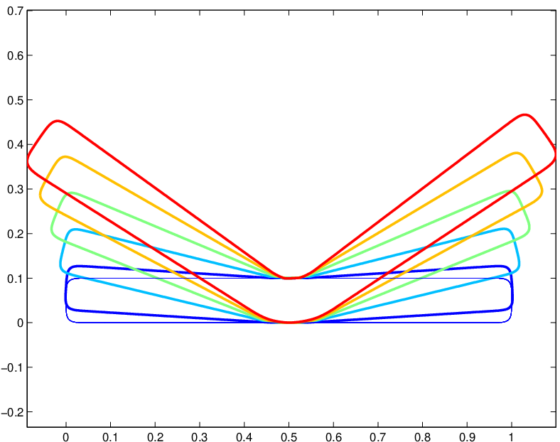
λ=.01\lambda=.01 λ=50\lambda=50
Refer to caption
λ=300\lambda=300 λ=2000\lambda=2000
Figure 4: Piecewise similarity Finsler flow evolutions for ρ=0.3\rho=0.3 and for different values of λ\lambda.

Influence of λ\lambda.

We first re-use the synthetic example introduced in Section 7.1 to illustrate the influence of the parameter λ\lambda. We thus use an evolution driven by the flow F⁡(Γ)∈TΓ​ℬF(\Gamma)\in T_{\Gamma}\mathscr{B} defined in (7.1). Figure 4 shows how λ\lambda allows one to interpolate between the piecewise rigid model (when λ=0\lambda=0) to a piecewise similarity model when λ\lambda increases. For large value of λ\lambda, one clearly sees the global scaling introduced by the model which is helpful to better follow the flow of FF.

Figure 5 compares the evolution obtained with the initial flow (7.2) (corresponding to (ρ,λ)=(0,0)(\rho,\lambda)=(0,0), i.e. the Finsler gradient is equal to F⁡(Γ)F(\Gamma)), the piecewise rigid flow (corresponding to ρ>0\rho>0 and λ=0\lambda=0) and the piecewise similarity flow (corresponding to ρ>0\rho>0 and λ>0\lambda>0).

Refer to caption Refer to caption
L2L^{2} (ρ,λ)=(0.5,0)(\rho,\lambda)=(0.5,0) (ρ,λ)=(0.5,200)(\rho,\lambda)=(0.5,200)
Figure 5: From left to right: evolutions by using the L2L^{2} gradient, piecewise rigid Finsler gradient, piecewise similarity Finsler gradient.

Application to the matching problem.

We now show an application of the Finsler descent method to the curve matching problem, by minimizing the energy EE defined in (5.4). Figure 6 shows the results obtained with the piecewise similarity penalty for well chosen parameters (σ,δ,λ,ρ)(\sigma,\delta,\lambda,\rho). These evolutions should be compared with the ones reported in Section 7.2. Allowing the length of the curve to vary using a parameter λ>0\lambda>0 allows the evolutions to better capture the geometry of the target shape and thus leads to better matchings.

Refer to caption Refer to caption Refer to caption
Refer to caption Refer to caption Refer to caption Refer to caption
Figure 6: Curve matching by piecewise similarity motions. Each image displays the target curve Λ\Lambda (dash line) and the current curve Γk\Gamma_{k} (solid line). We used the following parameters: top row: σ=0.8\sigma=0.8, δ=0.04\delta=0.04, λ=2000\lambda=2000, ρ=0.85\rho=0.85 ; middle row: σ=0.8\sigma=0.8, δ=0.08\delta=0.08, λ=2000\lambda=2000, ρ=0.95\rho=0.95 ; bottom row: σ=0.9\sigma=0.9, δ=0.03\delta=0.03, λ=2000\lambda=2000, ρ=0.87\rho=0.87.

Conclusion

This paper has presented a novel way to encode piecewise regular constraints for curve evolutions. This is achieved by designing Finsler penalties in the tangent space of curves. This method offers a unifying treatment of this class of evolutions. A distinctive feature of this approach is that it uses a convex modeling of the geometric constraints. For the particular case of piecewise rigid and piecewise similarity transforms, this avoids the need to specify the location of the articular points, which is a difficult problem. Instead, these articulations are obtained, at each iteration, through the resolution of a convex program. This novel method opens the doors to many fascinating theoretical questions, such as the definition of a continous flow when letting τk→0\tau_{k}\rightarrow 0, and the properties of Finslerian spaces of curves.

Acknowledgment

This work has been supported by the European Research Council (ERC project SIGMA-Vision).

9 Appendix: B​VBV and B​V2BV^{2} functions

In this section we remind the definition of B​VBV and B​V2BV^{2} functions in dimension one.

Definition 9.1.

Let u∈L1​([0,1],ℝ)u\in L^{1}([0,1],\mathbb{R}). We say that u is a function of bounded variation in [0,1][0,1] if

|Du|([0,1])=sup{∫01ug′dx:g∈Cc∞([0,1],ℝ),∥g∥L∞​([0,1],ℝ)⩽1}<∞.|Du|([0,1])=\sup\left\{\int_{0}^{1}u\,g^{\prime}\,\mathrm{d}x\;:\;g\in\mathrm{C}^{\infty}_{c}([0,1],\mathbb{R}),\|g\|_{L^{\infty}([0,1],\mathbb{R})}\leqslant 1\right\}<\infty\,. (9.1)

By Riesz’s representation theorem this is equivalent to state that there exists a unique finite Radon measure, denoted by D​uDu, such that

∫01ug′dx=−∫01gdDu∀g∈Cc1([0,1]).\int_{0}^{1}u\,g^{\prime}\,\mathrm{d}x=-\int_{0}^{1}g\,\mathrm{d}Du\quad\forall\,g\in\mathrm{C}^{1}_{c}({[0,1]})\,.

Clearly the total variation of the measure D​uDu on [0,1][0,1], i.e., |D​u|​([0,1])|Du|([0,1]), coincides with the quantity defined in (9.1) and this justifies our notations. We denote the space of functions of bounded variation in [0,1][0,1] by B​V​([0,1],ℝ)BV([0,1],\mathbb{R}). The space B​V​([0,1],ℝ)BV([0,1],\mathbb{R}) equipped with the norm

‖u‖B​V=‖u‖L1+|D​u|([0,1])\|u\|_{BV}=\|u\|_{L^{1}}+|Du|([0,1])

is a Banach space. We say that {uh}\{u_{h}\} weakly* converges in B​V​([0,1],ℝ)BV([0,1],\mathbb{R}) to uu if

uh​⟶L1​uandD​uh​⇀∗​D​u,ash→∞.u_{h}\overset{L^{1}}{\longrightarrow}u\quad\mbox{and}\quad Du_{h}\overset{*}{\rightharpoonup}Du\,,\quad\mbox{as}\quad h\rightarrow\infty\,.

We now define the set of B​V2BV^{2}-functions as the functions whose second derivative are Radon measures:

Definition 9.2.

Let u∈W1,1​([0,1],ℝ)u\in W^{1,1}([0,1],\mathbb{R}). We say that uu belongs to B​V2​([0,1],ℝ)BV^{2}([0,1],\mathbb{R}) if

|D2u|([0,1]):=sup{∫01ug′′dx:g∈Cc∞([0,1],ℝ),∥g∥L∞​([0,1],ℝ)⩽1}<∞.|D^{2}u|([0,1]):=\sup\left\{\int_{0}^{1}u\,g^{\prime\prime}\,\mathrm{d}x\;:\;g\in\mathrm{C}^{\infty}_{c}({[0,1]},\mathbb{R}),\|g\|_{L^{\infty}([0,1],\mathbb{R})}\leqslant 1\right\}<\infty\,. (9.2)

As for the first variation, the functional considered in (9.2) can be represented by a measure D2​uD^{2}u whose total variation coincides with the quantity |D2​u|​([0,1])|D^{2}u|([0,1]) previously defined.

B​V2​([0,1],ℝ)BV^{2}([0,1],\mathbb{R}) equipped with the norm

‖u‖B​V2=‖u‖B​V+|D2​u|([0,1])\|u\|_{BV^{2}}=\|u\|_{BV}+|D^{2}u|([0,1]) (9.3)

is a Banach space. In particular we have W2,1​([0,1],ℝ)⊂B​V2​([0,1],ℝ)W^{2,1}([0,1],\mathbb{R})\subset BV^{2}([0,1],\mathbb{R}). We say that {uh}\{u_{h}\} weakly* converges in B​V2​([0,1],ℝ)BV^{2}([0,1],\mathbb{R}) to uu if

uh​⟶W1,1​uandD2​uh​⇀∗​D2​u,ash→∞.u_{h}\overset{W^{1,1}}{\longrightarrow}u\quad\mbox{and}\quad D^{2}u_{h}\overset{*}{\rightharpoonup}D^{2}u\,,\quad\mbox{as}\quad h\rightarrow\infty\,.

We remind that if {uh}⊂B​V2​([0,1],ℝ)\{u_{h}\}\subset BV^{2}([0,1],\mathbb{R}) is such that supℎ​‖uh‖B​V2<M\underset{h}{\sup}\,\|u_{h}\|_{BV^{2}}<M then there exists u∈B​V2​([0,1],ℝ)u\in BV^{2}([0,1],\mathbb{R}) and a subsequence (not relabeled) {uh}\{u_{h}\} that weakly* converges in B​V2​([0,1],ℝ)BV^{2}([0,1],\mathbb{R}) toward uu and

|D2​u|​([0,1])⩽lim infh→∞​|D2​uh|​([0,1]).|D^{2}u|([0,1])\leqslant\,\underset{h\rightarrow\infty}{\liminf}\,|D^{2}u_{h}|([0,1])\,.

Moreover we have the following proposition showing the link between B​VBV and B​V2BV^{2} functions

Proposition 9.3.

A function uu belongs to B​V2​([0,1],ℝ)BV^{2}([0,1],\mathbb{R}) if and only if u∈W1,1​([0,1],ℝ)u\in W^{1,1}([0,1],\mathbb{R}) and u′∈B​V​([0,1],ℝ)u^{\prime}\in BV([0,1],\mathbb{R}), for every i=1,…,ni=1,...,n. Moreover

|D2​u|​([0,1])=|D​u′|​([0,1]).|D^{2}u|([0,1])=\left|Du^{\prime}\right|([0,1])\,.

We also remind that B​V2​([0,1],ℝ)BV^{2}([0,1],\mathbb{R}) is embedded in W1,∞​([0,1],ℝ)W^{1,\infty}([0,1],\mathbb{R}) so B​V2BV^{2} functions are Lipschitz continuous (see Theorem 5, [19] pag. 131). Then, as [0,1]⊂ℝ[0,1]\subset{\mathbb{R}} is bounded, B​V2​([0,1],ℝ)BV^{2}([0,1],\mathbb{R}) is embedded W1,p​([0,1],ℝ)W^{1,p}([0,1],\mathbb{R}), for every p⩾1p\geqslant 1. In particular this implies that B​V2​([0,1],ℝ)BV^{2}([0,1],\mathbb{R}) is dense in W1,p​([0,1],ℝ)W^{1,p}([0,1],\mathbb{R}), for every p⩾1p\geqslant 1.

A vector field 𝐮{\bf u} belongs to B​V​([0,1],ℝ2)BV([0,1],\mathbb{R}^{2}) (B​V2​([0,1],ℝ2)BV^{2}([0,1],\mathbb{R}^{2}) respectively) if every component of 𝐮{\bf u} belongs to B​V​([0,1],ℝ)BV([0,1],\mathbb{R}) (B​V2​([0,1],ℝ)BV^{2}([0,1],\mathbb{R}) respectively). We refer to [3] and [18] for more properties of these spaces.

References

  • [1] P.-A. Absil, R. Mahony, and R. Sepulchre. Optimization on manifolds: Methods and applications. Recent Advances in Optimization and its Applications in Engineering. The 14th Belgian-French-German Conference on Optimization. Springer, pages 125–144, 2010.
  • [2] Y. I. Alber, R. S. Burachik, and A. N. Iusem. A proximal point method for nonsmooth convex optimization problems in banach spaces. Abstract and Applied Analysis, 2(1–2):97–120, 1997.
  • [3] L. Ambrosio, N. Fusco, and D. Pallara. Functions of Bounded Variation and Free Discontinuity Problems. Oxford Science Publications, 2000.
  • [4] L. Ambrosio, N. Gigli, and L. Savaré. Gradient Flows in Metric Spaces and in Spaces of the Probability Measures. Birkhäuser, 2008.
  • [5] K. Aoyama, F. Kohsaka, and W. Takahashi Abstract. Proximal Point Methods For Monotone Operators In Banach Spaces. Taiwanese Journal of Mathematics, 15(1):259–281, 2011.
  • [6] N. Aronszajn. Theory of reproducing kernels. Trans. Am. Math. Soc., 68(3):337–404, 1950.
  • [7] J. Ashburner. A fast diffeomorphic image registration algorithm. NeuroImage, 38(1):95–113, 2007.
  • [8] D. Bao, S.S. Chern, and Z. Shen. An introduction to Riemaniann-Finsler geometry. Springer-Verlag New York, Inc., 2000.
  • [9] S. Boyd and L. Vandenberghe. Convex optimization. Cambridge University Press, 2004.
  • [10] H. Brezis. Functional Analysis, Sobolev Spaces, and Partial Differential Equations. Springer, 2010.
  • [11] V. Caselles, R. Kimmel, and G. Sapiro. Geodesic active contours. International Journal of Computer Vision, 22(1):61–79, 1997.
  • [12] T. Chan and L. Vese. Active contours without edges. IEEE Transactions on Image Processing, 10(2):266–277, 2001.
  • [13] W. Chang and M. Zwicker. Automatic registration for articulated shapes. Computer Graphics Forum (Proceedings of SGP 2008), 27(5):1459–1468, 2008.
  • [14] G. Charpiat, R. Keriven, J. P. Pons, and O. D. Faugeras. Designing spatially coherent minimizing flows for variational problems based on active contours. Proc. ICCV, 2:1403–1408, 2005.
  • [15] G. Charpiat, P. Maurel, J. P. Pons, R. Keriven, and O. D. Faugeras. Generalized Gradients: Priors on Minimization Flows. International Journal of Computer Vision, 73(3):325–344, July 2007.
  • [16] Y. Chen and G. Medioni. Object modeling by registration of multiple range images. Proc. Conf. on Robotics and Automation, pages 2724–2729, 1991.
  • [17] F.H. Clarke. On the inverse function theorem. Pacific J. Math., 64(1):97–102, 1976.
  • [18] F. Demengel. Fonctions à hessien borné. Annales de l’Institut Fourier, 34(2):155–190, 1984.
  • [19] L. Evans and R.F. Garipey. Measure theory and fine properties of functions. CRC Press, 1992.
  • [20] G. Gilboa and S. Osher. Nonlocal linear image regularization and supervised segmentation. SIAM Multiscale Modeling and Simulation, 6:595–630, 2007.
  • [21] J. Glaunes, A. Trouvé, and L. Younes. Diffeomorphic matching of distributions : A new approach for unlabelled point-sets and sub-manifolds matching. Proc. of CVPR’04, 2:712–718, 2004.
  • [22] P. Harms and A. Mennucci. Geodesics in infinite dimensional Stiefel and Grassmann manifolds. Compte Rendus de l’Acadámie des Sciences, 350(15?16):773–776, 2012.
  • [23] A. Herbulot, S. Jehan Besson, S. Duffner, M. Barlaud, and G. Aubert. Segmentation of vectorial image features using shape gradients and information measures. Journal of Mathematical Imaging and Vision, 25:365–386, 2006.
  • [24] M. Hinze, R. Pinnau, M. Ulbrich, and S. Ulbrich. Optimization with PDE-Constraints. Springer, 2008.
  • [25] M. Kass, A. Witkin, and D. Terzopoulos. Snakes: Active contour models. International Journal of Computer Vision, 1(4):321–331, January 1988.
  • [26] M. Kilian, N.J. Mitra, and H. Pottmann. Geometric modeling in shape space. ACM Transactions on Graphics, 26(3):1–8, 2007.
  • [27] J. Kim, J.W. Fisher, A. Yezziand, M. Cetin, and A.S. Willsky. A nonparametric statistical method for image segmentation using information theory and curve evolution. IEEE Trans. Image Proc., 14:486–502, 2005.
  • [28] R. Malladi, J. A. Sethian, and B. C. Vemuri. Shape modeling with front propagation: A level set approach. IEEE Trans. Patt. Anal. and Mach. Intell., 17(2):158–175, 1995.
  • [29] A.C. Mennucci. Level set and PDE based reconstruction methods: Applications to inverse problems and image processing. Lecture Notes in Mathematics, Lectures given at the C.I.M.E. Summer School held in Cetraro, 8-13 September 2008, Springer-Verlag, 2013.
  • [30] P.W. Michor and D. Mumford. Riemannian geometries on spaces of plane curves. J. Eur. Math. Soc., 8(1):1–48, 2006.
  • [31] D. Mumford and J. Shah. Optimal approximations by piecewise smooth functions and associated variational problems. Communications on Pure and Applied Mathematics, XLII(4), 1989.
  • [32] K. Ni, X. Bresson, T.F. Chan, and S. Esedoglu. Local histogram based segmentation using the Wasserstein distanc. International Journal of Computer Vision, 84:97–111, 2009.
  • [33] J. Nocedal and S.J. Wright. Numerical optimization. Springer, 1999.
  • [34] W. Ring and B. Wirth. Optimization methods on Riemannian manifolds and their application to shape space. SIAM Journal on Optimization, 22(2):596–627, 2012.
  • [35] L. Risser, F.-X. Vialard, R. Wolz, M. Murgasova, D. Holm, and D. Rueckert. Simultaneous multiscale registration using large deformation diffeomorphic metric mapping. IEEE Transactions on Medical Imaging, 30(10):1746–1759, 2011.
  • [36] C.R. Shelton. Morphable surface models. Int. J. Comput. Vision, 38(1):75–91, June 2000.
  • [37] A. Sotiras, C. Davatzikos, and N. Paragios. Deformable medical image registration: A survey. IEEE Trans. Med. Imaging, 32(7):1153–1190, 2013.
  • [38] G. Sundaramoorthi, J.D. Jackson, A. J. Yezzi, and A. C. Mennucci. Tracking with Sobolev active contours. Proc. CVPR, 1:674–680, 2006.
  • [39] G. Sundaramoorthi, A.C.G. Mennucci, S. Soatto, and A. Yezzi. A new geometric metric in the space of curves, and applications to tracking deforming objects by prediction and filtering. SIAM J. Imaging Sciences, 4(1):109–145, 2011.
  • [40] G. Sundaramoorthi, A. J. Yezzi, and A. C. Mennucci. Sobolev Active Contours. International Journal of Computer Vision, 73(3):345–366, July 2007.
  • [41] G. Sundaramoorthi, A. J. Yezzi, and A. C. Mennucci. Properties of Sobolev-type metrics in the space of curves. Interfaces and Free Boundaries, 10(4):423–445, 2008.
  • [42] G. Sundaramoorthi, A. J. Yezzi, A. C. Mennucci, and G. Sapiro. New Possibilities with Sobolev Active Contours. International Journal of Computer Vision, 84(2):113–129, August 2009.
  • [43] A. Trouvé and F.-X. Vialard. Shape splines and stochastic shape evolutions: A second order point of view. Quarterly of Applied Mathematics, 70:219–251, 2012.
  • [44] M. Vaillant and J. Glaunès. Surface matching via currents. Information Processing in Medical Imaging, Lecture Notes in Computer Science, 3565:381–392, 2005.
  • [45] M. Vaillant, M. I Miller, L. Younes, and A. Trouvé. Statistics on diffeomorphisms via tangent space representations. NeuroImage, 23(1):161–169, 2004.
  • [46] Tom Vercauteren, Xavier Pennec, Aymeric Perchant, and Nicholas Ayache. Diffeomorphic demons: Efficient non-parametric image registration. NeuroImage, 45(1, supplement 1):S61–S72, 2009.
  • [47] G. Wahba. Spline models for observational data. CBMS-NSF Regional conference series. SIAM, 1990.
  • [48] A. Yezzi and A. Mennucci. Conformal metrics and true “gradient flows” for curves. Proc. ICCV, 1:913–919, 2005.
  • [49] A. Yezzi and A. Mennucci. Metrics in the space of curves. arXiv:math/0412454v2, 2005.
  • [50] L. Younes. Computable elastic distances between shapes. SIAM Journal of Applied Mathematics, 58(2):565–586, 1998.
  • [51] L. Younes, P.W. Michor, J. Shah, and D. Mumford. A metric on shape space with explicit geodesics. Rend. Lincei Mat. Appl., 19(1):25–57, 2008.