Route Swarm: Wireless Network
Optimization through Mobility

Consider a system of $n=m+s$ agents consisting of $m$ mobile robots indexed by $\mathcal{I}_{M}\triangleq\{1,\ldots,m\}$, and $s$ static sensors indexed by $\mathcal{I}_{S}\triangleq\{m+1,\ldots,m+s\}$. The mobile robots are assumed to have single integrator dynamics

where $x_{i},u_{i}\in\mathbb{R}^{2}$ are the position and the velocity control input for an agent $i\in\mathcal{I}_{M}$, respectively. Assume that all agents can intercommunicate in a proximity-limited way, inducing interactions (or topology) of a time varying nature. Specifically, letting $d_{ij}\triangleq\lVert x_{ij}\rVert\triangleq\lVert x_{i}-x_{j}\rVert$ denote the distance between agents $i$ and $j$, and $(i,j)$ a link between connected agents, the spatial neighborhood of each agent is partitioned by defining concentric radii $\rho_{2}>\rho_{1}>\rho_{0}$ as in Fig. 1, where we refer to $\rho_{2},\rho_{1},\rho_{0}$ as the interaction, connection, and collision avoidance radii, respectively. The radii introduce a hysteresis in interaction by assuming that links $(i,j)$ are established only after $d_{ij}\leq\rho_{1}$, with link loss then occurring when $d_{ij}>\rho_{2}$, generating the annulus of $\rho_{2}-\rho_{1}$ where decisions on link additions and deletions are made (c.f. Section V-A).

The above spatial interaction model is formalized by the undirected dynamic graph, $\mathbb{G}=(\mathcal{V},\mathcal{E})$, with vertices (nodes) $\mathcal{V}$ indexed by $\mathcal{I}_{M}\cup\mathcal{I}_{S}$ (the agents), and edges $\mathcal{E}\subseteq\mathcal{V}\times\mathcal{V}$ such that $(i,j)\in\mathcal{E}\Leftrightarrow(\lVert x_{ij}\rVert\leq\rho_{2})\;\wedge\;\sigma_{ij}$, with switching signals [15]:

where $(i,i)\notin\mathcal{E}$ (no self-loops) and $(i,j)\in\mathcal{E}\Leftrightarrow(j,i)\in\mathcal{E}$ (symmetry) hold for all $i,j\in\mathcal{V}$. Nodes with $(i,j)\in\mathcal{E}$ are called neighbors and the neighbor set for an agent $i$ is denoted $\mathcal{N}_{i}=\{j\in\mathcal{V}\,|\,(i,j)\in\mathcal{E}\}$.

From the set of static sensors $\mathcal{I}_{S}$ we construct $f$ information flows indexed by $\mathcal{I}_{F}\triangleq\{n+1,\ldots,n+f\}$, each consisting of source-destination pairs defining a desired flow of network information. For a given flow $i\in\mathcal{I}_{F}$, we use the following notation: $\mathcal{F}_{i}\in\mathcal{I}_{S}\times\mathcal{I}_{S}$ represents the source and destination nodes for flow $i$, with $\mathcal{F}_{i}^{s}\in\mathcal{I}_{S}$ and $\mathcal{F}_{i}^{d}\in\mathcal{I}_{S}$ representing source and destination indices, respectively. Further, for convenience we use notation $x_{i}^{s},x_{i}^{d}\in\mathbb{R}^{2}$ to represent the position of the source and destination for the flow $i\in\mathcal{I}_{F}$. The set of flow pairs is denoted $\mathcal{F}\triangleq\{\mathcal{F}_{1},\ldots,\mathcal{F}_{f}\}$. At any time, a subset of these static pairs is active, forming the set of active flows $\mathcal{I}_{F}$, calling for dynamic configurability of the hybrid network, our contribution in this work. Thus, at a high level our system objective is to facilitate information flow for each source/destination pair by configuring the mobile robots such that each flow is connected and is at least approximately optimal in terms of data transmission, and that the entire network itself $\mathbb{G}$ is connected to guarantee complete network collaboration.

To measure link quality towards optimizing a given flow, we assume that each $(i,j)\in\mathcal{E}$ has a weight parameter $w_{ij}$ that describes their cost with respect to transmitting information. A commonly used metric for link quality is ETX, i.e. the expected number of transmissions per successfully delivered packet. This can be modeled as the inverse of the successful packet reception rate $\lambda_{ij}$ over the link. As the expected packet reception rate has been empirically observed and analytically shown to be a sigmoidal function of distance decaying from 1 to 0 as distance $d_{ij}$ is increased [16], it can be modeled as follows:

where $a,b\in\mathbb{R}_{+}$ are shape and center parameters depending on the communication range and the variance of environmental fading. Accordingly, the link weights $w_{ij}$, if chosen to represent ETX, can be modeled as a convex function of the inter-node distance $d_{ij}$:

The cost for flow $k\in\mathcal{I}_{F}$ is then taken to be the sum of ETX values on the path of the flow, i.e.:

where we apply notation $\mathbb{G}_{F}^{k}=(\mathcal{V}_{F}^{k},\mathcal{E}_{F}^{k})$ as the graph defining the interconnection over flow $k\in\mathcal{I}_{F}$ (we give a concrete definition of flow membership in Section IV-A). Our problem in this work is then formalized as follows:

In solving the connectivity constrained version of the flow optimization of Theorems IV.1, IV.2, and IV.3, due to problem complexity we provide a heuristic algorithm to solve the inter-flow allocation problem, leaving the intra-flow optimization to the PCP (Section V). Algorithm 1 depicts the high-level components of the proposed heuristic, each of which is detailed in the sequel.

To begin, we define the flow membership for an agent as $i\in\mathcal{I}_{M}$ as $\mathcal{M}_{i}\in\mathcal{I}_{F}$, where the set of memberships is denoted as $\mathcal{M}\triangleq\{\mathcal{M}_{1},\ldots,\mathcal{M}_{n}\}$. We denote with $\mathbb{G}_{F}^{i}=(\mathcal{V}_{F}^{i},\mathcal{E}_{F}^{i})$ the graph defining the interconnection over flow $i\in\mathcal{I}_{F}$ of agents $j\in\mathcal{I}_{S}\cup\mathcal{I}_{M}$ with $i\in\mathcal{M}_{j}$. Thus we have $\mathcal{V}_{F}^{i}=\{j\in\mathcal{I}_{S}\cup\mathcal{I}_{M}\,|\,i\in\mathcal{M}_{j}\}$ and $(j,k)\in\mathcal{E}_{F}^{i}\Leftrightarrow(i\in\mathcal{M}_{j}\cap\mathcal{M}_{k})\wedge(j\in\mathcal{N}_{k})$, with $k\in\mathcal{I}_{S}\cup\mathcal{I}_{M}$. Notice that by definition $\mathbb{G}_{F}^{i}\subseteq\mathbb{G}$. We will also refer to the collection of flow graphs simply by $\mathbb{G}_{F}$. We also have flow neighbors defined as $\mathcal{N}_{i}^{F}=\{j\in\mathcal{N}_{i}\,|\,\mathcal{M}_{j}\cap\mathcal{M}_{i}\neq\emptyset\}$. Furthermore, we denote with $\mathcal{D}_{i}\in\mathcal{I}_{M}$ the detachable agents $j\in\mathcal{I}_{M}$ for flow $i\in\mathcal{I}_{F}$, i.e. those agents for which reconfiguration does not impact network connectedness. The set of detachments is denoted by $\mathcal{D}\triangleq\{\mathcal{D}_{1},\ldots,\mathcal{D}_{f}\}$.

Due to the system connectivity constraint, the ICP is not free to select any mobile agent for flow reallocation, specifically as intra-flow connectivity or overall flow-to-flow connectivity may be lost. Thus, the ICP must detect bridges, i.e., mobile nodes whose reconfiguration might break flow-to-flow connectivity over the network, and also consider safe detachments (flow-to-flow motion), i.e., a node whose reconfiguration in the workspace does not impact the connectivity of the source flow.

Respecting our connectivity constraint, we first detect initial flow membership by computing the shortest path (in terms of link cost) for each source/destination pair per flow by using for example Dijkstra’s algorithm (lines 3-5 of Algorithm 1). This defines the connected backbone for each flow implicitly identifying the mobile nodes required to maintain flow-connectivity. Additionally, we have optimality of the connected flow backbones as we maximize the link utility (or minimize path costs) between source and destination nodes.

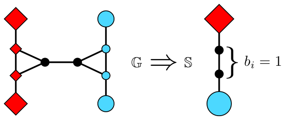
In detecting bridge agents we follow the process outlined by Algorithms 2, 3, and 4, where we denote by $b_{i}\in\{0,1\}$ the status of agent $i\in\mathcal{I}_{S}\cup\mathcal{I}_{M}$ as a connectivity preserving bridge, with $b=\{b_{1},\ldots,b_{n}\}$. Briefly speaking, the primary problem of this process is the construction of a supergraph, denoted $\mathbb{S}=(\mathcal{V}_{\mathbb{S}},\mathcal{E}_{\mathbb{S}})$, defining the interconnection of the flows. In this way, we can identify nodes which are critical in defining the flow-to-flow connectivity over the system. Figure 2 depicts an example of supergraph construction. We first add one node for each flow in the system, and then we add a node for each non-flow member in the system that represents potential bridge candidates. Edges between non-flow members are preserved, while there is only one edge between any given non-flow member and the node which represents a flow in the supergraph. Bridges can then be simply detected as the members of the shortest path between any pair of nodes representing flows in the supergraph (e.g. Fig. 2), where connectivity is guaranteed by construction:

In order to control the properties of $\mathbb{G}$ (i.e. connectivity) we exploit the constrained interaction framework proposed by Williams and Sukhatme in [9]. The constrained interaction framework acts through hysteresis (2) to regulate links spatially with simple application of attraction and repulsion to retain established links or reject new links with respect to topological constraints. Define the discernment region $\lVert x_{ij}\rVert\in(\rho_{1},\rho_{2}]$, where agent $i$ decides relative to system constraints (here connectivity) whether agent $j$ is a candidate for link addition ($j\notin\mathcal{N}_{i}$) or deletion ($j\in\mathcal{N}_{i}$), or if agent $j$ should be attracted (retain $(i,j)\in\mathcal{E}$) or repelled (deny $(i,j)\notin\mathcal{E}$). Define predicates for link addition and deletion, $P_{ij}^{a},P_{ij}^{d}:\mathcal{V}\times\mathcal{V}\rightarrow\{0,1\}$, activated at $\rho_{2}$ and $\rho_{1}$, respectively, that indicate constraint violations if the link $(i,j)$ were allowed to be either created or destroyed, i.e. $\lVert x_{ij}\rVert$ transits $\rho_{1}$ or $\rho_{2}$. The predicates designate for the $i$th agent the membership of nearby agents in link addition and deletion candidate sets $\mathcal{C}_{i}^{a},\mathcal{C}^{d}_{i}$, and attraction and repulsion sets $\mathcal{D}_{i}^{a},\mathcal{D}_{i}^{r}$. Link control is then achieved by choosing control $u_{i}$ having attractive and repulsive potential fields between members of $\mathcal{D}_{i}^{a},\mathcal{D}_{i}^{r}$, respectively.

In particular, to regulate network topology spatially, we design the agent controls as follows:

with potentials $\psi_{ij}^{a},\psi_{ij}^{r},\psi_{ij}^{c}\colon\mathbb{R}_{+}\rightarrow\mathbb{R}_{+}$, serving the purposes of attraction, repulsion, and collision avoidance, where $\Pi_{i}=\{j\in\mathcal{V}\,|\,\lVert x_{ij}\rVert\leq\rho_{0}\}$ is the collision avoidance set for agent $i$. Further, each agent can also apply (based on $\mathcal{S}_{i}$) an exogenous objective (i.e. non-cooperative) controller $u_{i}^{e}\in\mathbb{R}^{2}$ and an inter-agent coordination objective $u_{i}^{o}\in\mathbb{R}^{2}$ (e.g. dispersion as will be seen in Section V-D). An appropriate attractive potential which we adopt for this work takes the following form:

where $\Psi_{a}(\lVert x_{ij}\rVert)$ is chosen such that (11) is smooth over the $\rho_{1}$ transitions. Similar to the attractive potential (11), the repulsive potential takes the form

where $\Psi_{r}$ is chosen to guarantee $\psi_{ij}^{r}$ is smooth over the $\rho_{2}$ transition. Finally, a basic collision avoidance is given by potential

with $\Psi_{r}$ chosen to guarantee $\psi_{ij}^{c}$ is smooth over the $\rho_{0}$ transition.

The attractive and repulsive potentials are constructed such that $\psi_{ij}^{a}\rightarrow\infty$ as $d_{ij}\rightarrow\rho_{2}$ and $\psi_{ij}^{r}\rightarrow\infty$ as $d_{ij}\rightarrow\rho_{1}$, guaranteeing link retention and denial, respectively, and allowing us through predicates $P_{ij}^{a},P_{ij}^{d}$ to control desired properties of $\mathbb{G}$ (e.g. connectivity).

Notice that in maintaining network connectivity, we require only link retention action, allowing us to immediately choose

for the link addition predicates, effectively allowing link additions to occur between all interacting agents across all network states³³ 3 Although in this work we allow all link additions, link addition control could be useful for example in regulating neighborhood sizes to mitigate spatial interference, or to disallow interaction between certain agents..

Now, in accordance with Algorithm 7, the link deletion predicates are given by:

where by assumption $i,j\in\mathcal{I}_{M}$, i.e. only mobile agents apply controllers. We choose link retention (15) to guarantee that connectivity is maintained both within flows across $\mathbb{G}_{F}$, and from flow to flow across bridge agents over the supergraph $\mathbb{S}$, noting that idle agents with $\mathcal{M}_{i}=\emptyset$ and reconfiguring agents with $\mathcal{S}_{i}=\textit{RECONFIGURE}$ are free to lose links as they have been deemed redundant by the ICP with respect to network connectivity.

While maintaining connectivity as above, each agent further acts according to ICP reconfiguration commands towards optimizing inter-flow allocations. Specifically, in response to command $\mathcal{C}_{i}$, agent $i$ enters the reconfiguration state $\mathcal{S}_{i}\leftarrow\textit{RECONFIGURE}$, and begins to apply a waypoint controller as follows (c.f. lines 4-7 of Algorithm 7). When $\mathcal{S}_{i}=\textit{RECONFIGURE}$, agent $i$ applies exogenous objective controller

where $x^{w}\in\mathbb{R}^{2}$ is the target waypoint calculated as the midpoint of target flow $\mathcal{C}_{i}$.

The input (16) is a velocity damped waypoint seeking controller, having unique critical point $x_{i}\rightarrow x^{w}$ (i.e. a point at which $u_{i}^{e}=\mathbf{0}$), guaranteeing that the target intra-flow positioning (and thus membership) for agent $i$ is achieved. As the convergence of $x_{i}\rightarrow x^{w}$ is asymptotic in nature, to guarantee finite convergence and state switching, we apply a saturation $\lVert x^{w}-x_{i}\rVert\leq\epsilon^{w}$ with $0<\epsilon^{w}<<1$ to detect waypoint convergence, initiating a switch to $\mathcal{S}_{i}\leftarrow\textit{SWARMING}$ as in lines 23-25 of Algorithm 7.

Once the ICP has assigned flow memberships $\mathcal{M}_{i}\;\forall\;i\in\mathcal{I}_{M}$ and all commanded reconfigurations $\mathcal{C}_{i}$ have been completed, the mobile agents begin to seek to optimize the flow to which they are a member. First, we assume that flow members must configure along the line segment connecting flow source/destination pairs, yielding in the case of proximity-limited communication, a line-of-sight or beamforming style heuristic. The membership of an agent $i\in\mathcal{I}_{M}$ to a flow $j\in\mathcal{M}_{i}$ thus initiates a check to determine if $x_{i}$ lies on the flow path $x_{j}^{s}+\tau x_{j}^{d}$, within a margin $0<\epsilon_{F}<<1$ (c.f. lines 9-16, Algorithm 7). To do so, the projection of $x_{i}$ onto $x_{j}^{s}+\tau x_{j}^{d}$ is determined first by computing

defining whether the projection will lie within or outside of the flow path. Then we have the saturated projection

where $\alpha>0$ is a biasing term such that the projection does not intersect $x_{j}^{s}$ or $x_{j}^{d}$. We then have the state transition condition

which when satisfied gives $\mathcal{S}_{i}\leftarrow\textit{SWARMING}$ (line 14, Algorithm 7, and described below). If condition (19) is not satisfied, agent $i$ transitions to state $\mathcal{S}_{i}\leftarrow\textit{RECONFIGURE}$, applying waypoint controller (16) with $x^{w}\triangleq x_{i\rightarrow\mathcal{F}_{j}}$, guaranteeing a reconfiguration, in a shortest path manner, to a point on the line segment defining its assigned flow $\mathcal{M}_{i}$.

Finally, when an agent $i$ is in the swarming state $\mathcal{S}_{i}=\textit{SWARMING}$ (lines 18-20, Algorithm 7), after all necessary reconfigurations have been made (either by the ICP via $\mathcal{C}_{i}$ or internally by flow alignment), a dispersive inter-neighbor controller is applied in order to optimize the assigned flow. Specifically, each swarming agent $i\in\mathcal{I}_{M}$ applies a coordination controller (regardless of bridge status $b_{i}$):

where

is the set of neighbors that share membership in flow $\mathcal{M}_{i}$, and who are either in flow and actively swarming (i.e. by condition (19)), or are a static source/destination node. Further, we define

as the set of static in flow neighbors for which compensation (Remark V.1, below) must be applied. Controller (20) dictates that mobile flow members disperse equally only with fellow flow members and also with the source/destination nodes of their assigned flow $\mathcal{M}_{i}$.

While dispersive controllers generally yield equilibria in which inter-agent distant is maximized (up to $\rho_{2}$) [17], as each flow is constrained by static source/destination nodes, the dispersion (20) generates our desired equidistant intra-flow configuration as formalized below:

A formal proof is beyond the scope of this work⁴⁴ 4 Informally, an energy balancing argument establishes the result., however note that our controllers operate using only inter-agent distance, an advancement beyond related works such as [13].

References

- [1] V. Gazi and K. Passino, “Stability analysis of swarms,” Automatic Control, IEEE Transactions on, vol. 48, no. 4, pp. 692–697, 2003.
- [2] R. Olfati-Saber, “Flocking for multi-agent dynamic systems: algorithms and theory,” Automatic Control, IEEE Transactions on, vol. 51, no. 3, pp. 401–420, 2006.
- [3] J. Fax and R. Murray, “Information flow and cooperative control of vehicle formations,” Automatic Control, IEEE Transactions on, vol. 49, no. 9, pp. 1465–1476, 2004.
- [4] M. M. Zavlanos and G. J. Pappas, “Distributed connectivity control of mobile networks,” Trans. Rob., vol. 24, no. 6, pp. 1416–1428, Dec. 2008. [Online]. Available: http://dx.doi.org/10.1109/TRO.2008.2006233
- [5] R. K. Williams and G. S. Sukhatme, “Locally Constrained Connectivity Control in Mobile Robot Networks,” in IEEE International Conference on Robotics and Automation, 2013.
- [6] P. Yang, R. A. Freeman, G. J. Gordon, K. M. Lynch, S. S. Srinivasa, and R. Sukthankar, “Brief paper: Decentralized estimation and control of graph connectivity for mobile sensor networks,” Automatica, vol. 46, no. 2, pp. 390–396, Feb. 2010.
- [7] L. Sabattini, C. Secchi, N. Chopra, and A. Gasparri, “Distributed control of multiÐrobot systems with global connectivity maintenance,” Robotics, IEEE Transactions on, pp. 1–6, 2013.
- [8] D. Dimarogonas and K. Kyriakopoulos, “Connectedness preserving distributed swarm aggregation for multiple kinematic robots,” Robotics, IEEE Transactions on, vol. 24, no. 5, pp. 1213–1223, 2008.
- [9] R. Williams and G. Sukhatme, “Constrained interaction and coordination in proximity-limited multiagent systems,” Robotics, IEEE Transactions on, pp. 1–15, 2013.
- [10] G. Wang, G. Cao, P. Berman, and T. La Porta, “Bidding protocols for deploying mobile sensors,” Mobile Computing, IEEE Transactions on, vol. 6, no. 5, pp. 563–576, 2007.
- [11] A. Gasparri, B. Krishnamachari, and G. S. Sukhatme, “A framework for multi-robot node coverage in sensor networks,” Annals of Mathematics and Artificial Intelligence, vol. 52, no. 2-4, pp. 281–305, Apr. 2008.
- [12] N. Chatzipanagiotis, M. M. Zavlanos, and A. Petropulu, “A distributed algorithm for cooperative relay beamforming,” in American Control Conference, Washington, DC, June 2013.
- [13] D. K. Goldenberg, J. Lin, A. S. Morse, B. E. Rosen, and Y. R. Yang, “Towards mobility as a network control primitive,” in Proceedings of the 5th ACM international symposium on Mobile ad hoc networking and computing, ser. MobiHoc ’04. ACM, 2004, pp. 163–174.
- [14] Y. Yan and Y. Mostofi, “Robotic router formation in realistic communication environments,” Robotics, IEEE Transactions on, vol. 28, no. 4, pp. 810–827, 2012.
- [15] M. Ji and M. Egerstedt, “Distributed Coordination Control of Multiagent Systems While Preserving Connectedness,” IEEE Transactions on Robotics, vol. 23, no. 4, pp. 693–703, 2007.
- [16] M. Z. Zamalloa and B. Krishnamachari, “An analysis of unreliability and asymmetry in low-power wireless links,” ACM Trans. Sen. Netw., vol. 3, no. 2, Jun. 2007. [Online]. Available: http://doi.acm.org/10.1145/1240226.1240227
- [17] D. Dimarogonas and K. Kyriakopoulos, “Inverse agreement protocols with application to distributed multi-agent dispersion,” Automatic Control, IEEE Transactions on, vol. 54, no. 3, pp. 657–663, 2009.