The abelian confinement mechanism revisited: new aspects of the Georgi-Glashow model
Abstract:
The confinement problem remains one of the most difficult problems in theoretical physics. An important step toward the solution of this problem is the Polyakov’s work on abelian confinement. The Georgi-Glashow model is a natural testing ground for this mechanism which has been surprising us by its richness and wide applicability. In this work, we shed light on two new aspects of this model in D. First, we develop a many-body description of the effective degrees of freedom. Namely, we consider a non-relativistic gas of W-bosons in the background of monopole-instanton plasma. Many-body treatment is a standard toolkit in condensed matter physics. However, we add a new twist by supplying the monopole-instantons as external background field. Using this construction, we calculate the exact form of the potential between two electric probes as a function of their separation. This potential is expressed in terms of the Meijer-G function which interpolates between logarithmic and linear behavior at small and large distances, respectively. Second, we develop a systematic approach to integrate out the effect of the W-bosons at finite temperature in the range , where is the W-boson mass, starting from the full relativistic partition function of the Georgi-Glashow model. Using a heat kernel expansion that takes into account the non-trivial thermal holonomy, we show that the partition function describes a three-dimensional two-component Coulomb gas. We repeat our analysis using the many-body description which yields the same result and provides a check on our formalism. At temperatures close to the deconfinement temperature, the gas becomes essentially two-dimensional recovering the partition function of the dual sine-Gordon model that was considered in a previous work.
1 Introduction
After almost 60 years since Yang and Mills formulated their theory [1], color confinement remains one of the greatest puzzles in theoretical physics. Eventhough lattice gauge theories have been successful in demonstrating quark confinement in computer simulations, it is safe to say that up to date there is no analytical understanding of the confinement mechanism in dimensions. 11 1 See [2] for a recent review of the confinement problem, and [3] for the elements of the big picture. A breakthrough idea toward the solution of the confinement problem was introduced in the pioneering work of Polyakov [4], who showed that the proliferation of monopole-instantons in the vacuum of compact QED in dimensions leads to the confinement of electric charges. These monopoles are solution to the Euclidean classical equations of motion, and result due to the compact nature of the gauge group. Immediately after this work, Polyakov showed that the same confinement mechanism is at work in the Georgi-Glashow model 22 2 This model was proposed by Georgi and Galshow in the early seventies of the last century in the context of unified field theories [6]. in D [5]. This model consists of an Yang-Mills theory coupled to a triplet of scalar fields. 33 3 The generalization to gauge groups was worked out in [7]. Previously, it was shown in [8, 9] that this model admits finite non-singular and nonperturbative solutions to the classical equations of motion. These are the Polyakov ’t-Hooft magnetic monopoles in D, and monopole-instantons in the Euclidean setup in D. The monopole-instantons are charged under abelian group. This is the unbroken compact subgroup of the original , which breaks spontaneously upon giving a vacuum expectation value to the scalars. The monopole-instantons interact via Coulombic forces and form a gas of monopole plasma. In order to test the effect of the monopole proliferation on two external electric test charges, one computes the behavior of the Wilson loop in the background of the monopole plasma. The Wilson loop is a gauge invariant order parameter for confinement. Usually, we take our loops to be rectangles which represent the creation, propagation and annihilation of two charged probes separated a distance for time . In the confinement phase, the expectation value of the Wilson loop experiences an area-law behavior
| (1) |
where is the area of the loop enclosed by the curve , and is a proportionality constant interpreted as the string tension. In order to understand the area-law behavior, we can think of the Wilson loop as a current loop which itself generates a magnetic field. The monopole and anti-monopoles will line up along the area of the rectangular loop to screen out the generated magnetic field. Therefore, the area-law behavior is associated with the screening sheet of monopoles along the area of the loop.
A complementary way of thinking about the confinement mechanism is to consider the dual superconductivity picture advocated by ’t Hooft and Mandelstam [10, 11]. In superconductors, the condensation of electric charges, known as Cooper pairs, breaks the of electromagnetism spontaneously which in turn gives a mass to the photon. This is the Meissner effect which is responsible for screening the magnetic flux lines in superconductors. However, in type II superconductors magnetic field lines are allowed to exist in the form of flux tubes known as Abrikosov vortices [12]. If we place two magnetic monopoles in the bulk of a type II superconductor, the magnetic flux lines can not spread everywhere in the bulk. Instead, they collimate into a thin flux tube which can be though of a string connecting the two monopoles. Hence, at distance much larger than the screening length of the superconductor the potential between the probes will behave as , where is the string tension. According to ’t Hooft and Mandelstam, the vacuum of Yang-Mills behaves as type II superconductor except with a reversal of the rules of electric and magnetic charges. In fact, the Polyakov works [4, 5] are the first demonstration of the dual superconductivity picture. Later on, a beautiful implementation of this picture was worked out by Seiberg and Witten in D in a supersymmetric context [13, 14].
Since the pioneering work of Polyakov, the Georgi-Glashow model has been a testing ground not only for the confinement phenomena, but also for the deconfinement transition. Pure Yang-Mills theory in D experiences a deconfinement transition at strong coupling which hinders a full understanding of the transition [15]. Hence, one needs a simpler theory that resembles the original one, yet under analytic control. The finite temperature effects in the D Georgi-Glashow model were first considered in [16]. There, it was shown that a confinement-deconfinement transition happens at temperature , where is the Yang-Mills coupling constant. However, the authors in [16] ignored the effect of the W-bosons which plays an important role near the transition region, as was shown later on in [17]. Taking the W-bosons into consideration, the authors in [17] argued that the partition function near the transition region is that of a two-dimensional double Coulomb gas of monopole-instantons and W-bosons. This gas can be mapped into a dual sine-Gordon model which is further studied using bosonization/fermionization techniques. With such technology, it was shown that the inclusion of the W-bosons modifies the transition temperature to and that the transition is second order and belongs to the 2D Ising universality class. 44 4 Also see [18, 19] for reviews.
In this paper, we shed light on some issues that have not been considered before in the Georgi-Glashow model. In the first part of this work, we answer an important question which concerns the behavior of the potential between two external electric probes at intermediate distances. At distances much shorter then the screening length of the monopole-instanton plasma , the potential between the probes is logarithmic. On the other hand, at distances much larger than , the potential is linear. However, an analytic expression for the behavior of the potential in the intermediate region between the logarithmic and linear potential is still lacking. For this purpose, we develop a Euclidean many-body description of the partition function of the system. In this formalism, we consider the external electric probes as well as W-bosons in the background of the field generated by an arbitrary number of monopole-instantons. Since we are interested only in temperatures much lower than the mass of the W-bosons, we can limit ourselves to a non-relativistic description. Many-body treatment is a powerful tool in condensed matter systems. In the present work, we adapt this method to take into account the effect of monopole-instantons which, to the best of our knowledge, has not been considered elsewhere. At zero temperature, the W-bosons do not play any role thanks to the Boltzmann suppression factor . In this case, we can work only with a partition function that describes the external probes in the background of monopole-instanton gas. Further, we assume that the density of the instantons obey a Gaussian distribution. Although this introduces an error in the string tension, such an assumption considerably simplifies our computations. We find that the potential between two probes of charges separated a distance is expressed in terms of the Meijer-G function
which smoothly transits from logarithmic behavior at distances to a linear potential at distances much larger than the screening length. This behavior is illustrated in Figure (1) where we plot the potential and electric field as a function of the separation distance .
In the second part of our work, we perform a systematic study of the finite-temperature partition function of the Georgi-Glashow model in the temperature range , where is the W-boson mass. In this regard, we take two different approaches. In the first approach, we start our treatment from the full relativistic partition function which treats the monopole-instantons as external background field, and then apply a heat kernel expansion technique which takes into account the non-trivial thermal holonomy. This results in an effective action that contains both relevant and irrelevant operators. Ignoring the irrelevant ones, we show that the partition function of the system takes the form of the grand canonical distribution of a non-relativistic three-dimensional double Coulomb gas:
The gas consists of W-bosons and monopole-instantons with fugacities and , respectively. Two W-bosons carrying charges and located at interact logarithmically (which is the two-dimensional potential) at all temperatures in the range . While two monopole-instantons with charges and three-dimensional positions interact via , where is the Green’s function of the Laplacian operator on , and is the thermal circle. In addition, W-bosons interact with monopole-instantons via the Aharonov-Bohm phase . At temperatures much larger than the inverse distance between two-monopole instantons, yet much lower than the deconfinement temperature, the Green’s function reduces to a logarithmic function and the gas becomes essentially two-dimensional recovering the same partition function considered before in [17]. In the second approach, we start from the non-relativistic many-body description and then integrate out the W-bosons to recover (). This also works as an independent check which ensures the validity of our many-body description.
This paper is organized as follows. In Section 2, after a quick review of the Georgi-Glashow model, we write down the relativistic partition function of the system taking into account the monopole-instantons as background field. Then, motivated by a physical picture, we give a non-relativistic many-body description of the system. In Section 3, we use the many-body partition function, aided by a mean-field approach, to derive the potential between two static electric probes at zero temperature. In Section 4, we use both the relativistic and non-relativistic partition functions to show that the finite-temperature Georgi-Glashow model can be thought of as a three-dimensional double Coulomb gas as explained above. Finally, we conclude in Section 4 and provide directions for future research. The paper contains three appendices displaying miscellaneous calculations.
2 Theory and formulation
2.1 The Georgi-Glashow model: perturbative treatment
We consider the Lagrangian of Georgi-Glashow model in
| (6) |
where is the three-dimensional coupling constant, and are matter fields in the adjoint representation of the group. The Greek indices run from to and the color indices run from to . The field strength tensor and the covariant derivative are given by
| (7) |
The field acquires a vacuum expectation value (say in the direction) which breaks the down to . Then, we write the third component of the Higgs field as , where is the physical excitation of the Higgs field. The third color component of the gauge field remains massless, and the other two components form massive vector bosons:
| (8) |
The massive vector bosons, or W-bosons for short, carry electric charge , where . We also define the charged Goldstone Bosons as
| (9) |
Substituting (8) and (9) into (6), we find that the Lagrangian (6) can be rewritten as the sum of quadratic and interaction pieces :
| (10) | |||||
and
| (11) | |||||
where , and . At this stage, let us emphasize that the field does not only describe the photon fluctuations, but it can also include any external background fields, like the monopole-instanton field, as we will explain shortly.
The last line in the quadratic Lagrangian (10) has three terms that may add difficulties to our analysis. We can use integration by parts in the first term to get which is not in the form of a Klein-Gordon operator, i.e. . The other two terms couple the W-bosons to the Goldston bosons. Fortunately, one can get rid of these three terms by entertaining the fact that our Lagrangian has a gauge freedom. Therefore, by choosing an appropriate gauge we can eliminate the unwanted terms. To this end, we add the gauge fixing Lagrangian , where
| (12) |
Thus
| (13) |
It is clear that this gauge fixing Lagrangian eliminates the last three terms in (10). After gauge fixing, we also need to include the ghost contribution , where are the ghost fields. To calculate the quantity we proceed as follows. First, we note that the fields and transform under the infinitesimal gauge transformation as and . Then, we decompose into , the gauge parameter of the unbroken group, and along the and color directions. Hence, we obtain
| (14) |
Then, we find .
In the following, it is more appropriate to work in Euclidean space. A Euclidean version of the Lagrangian can be obtained by performing a Wick rotation. Adding the contribution from the gauge fixing and ghost terms, the total Lagrangian reads (from here on, we do not distinguish between upper and lower indices)
| (15) | |||||
where , and we have used where is the W-boson mass. Notice that the Lagrangian is invariant under the electromagnetic gauge group since the gauge fixing we have used leaves the subgroup of the intact.
This ends our treatment of the perturbative part. However, the Georgi-Glashow model contains also nonperturbative solutions. These are monopole-instantos that were first discovered by Polyakov [9] and ’t Hooft [8] as solitons in the Georgi-Glashow model in D. According to the path integral formulation of field theory, the grand partition function of the system is obtained by summing over all trajectories, that take us from one point in the field space to the other, weighted by their action:
| (16) |
This sum must include contributions from both perturbative and nonperturbative sectors. Before writing down the partition function of the Georgi-Glashow model, in the following section we review the nonperturbative solutions of the theory at hand.
2.2 Nonperturbative effects: adding monopole-instantons
In addition to the perturbative excitations described above, the three-dimensional Georgi-Glashow model admits nonperturbative objects. These are monopole-instantons allowed by the non-trivial homotopy , and are obtained as classical solutions to the Euclidean non-abelian equations of motion. These solutions have to be included in the path integral formulation of the field theory, which can have dramatic effects on the physics. Monopole-instantons are particle-like objects localized in space and time, have internal structure and mediate long range force, thanks to the unbroken . Although a single instanton solution satisfies the equations of motion, two or more instantons do not. However, if these objects are well separated, then a solution that is a superposition of many instantons can still be a good approximate solution to the equations of motion. In a reliable semi-classical treatment, one includes an arbitrary number of these objects in the path integral provided that they are well separated, or in other words, their density is low. This is known as the dilute gas approximation. In such approximation, the internal structure of the instantons does not play any role, and for all purposes we can replace the non-abelian field solution with an abelian one.
The abelian field of a single monopole-instanton localized at the origin is given by
| (17) |
where and are respectively the spatial and Euclidean time coordinates, and is the spherical-polar radius. The above solution is singular at . This is the Dirac string that stems from the location of the monopole-instanton at the origin and extends all the way along the negative -axis. This string is not physical; it is just a gauge artifact as can be shown directly by calculating the monopole field . The magnetic charge carried by a single monopole-instanton is defined as the surface integral of the monopole magnetic field over a 2-sphere, divided by :
| (18) |
In the dilute gas approximation, we add the contribution from an arbitrary number of these monopole-instantons that are randomly distributed all over the spacetime. This results in the total field
| (19) |
where is the position of the monopole-instanton and is its charge. Since monopole-instantons carry charges, they will interact via Coulombic forces. The form of interaction can be obtained from the action
| (20) |
where , and we have introduced the magnetic coupling
| (21) |
The electric and magnetic couplings are related by the Dirac quantization condition . This is twice the minimal value allowed for since the -bosons have twice the minimal charge.
Now, we are ready to include both perturbative and nonperturbative sectors in the path integral sum (16).
2.3 The grand partition function
The grand partition function of the system is obtained as a path integral over the fields , , , , and . Then, one includes the contribution from the nonperturbative sector as a sum over an arbitrary number of positive and negative monopole-instantons. Hence, the grand partition function reads
| (22) | |||||
where the monopole fugacity is given by 55 5 There is a typo in the pre-exponential factor of in the original work [5] which propagated to other places. The correct expression is given in [20], which we use here.
| (23) |
and is a function of the ratio between the W-boson mass and the Higgs mass. This function tends to unity in the Bogomolny-Prasad-Sommerfield (BPS) limit [21, 22], , and tends to in the opposite limit [23]. In the following, we assume that the Higgs mass is heavy and hence the Higgs field is short ranged and we can neglect its effects in our analysis. As we mentioned above, in order for the partition function to make sense, the monopole-instanton gas has to be dilute, or in other words . This in turn requires that we work in the weak coupling limit . Given the monopole fugacity , the average distance between two monopole-instantons is , apart from a dimensionfull pre-exponential factor.
It is very important to stress that the field appearing in the Lagrangian (15) is given by , and hence . Thus, includes contributions from both the fluctuations of the dynamical photon as well as the background field generated by the monopole-instantons. As a check that our formalism gives the standard monopoles interaction, we can turn off the photon field in (15) to find that , which is the monopole-monopole Coulomb interaction. In Section 4, it will be clear how to carry out the path integral rigorously by using an abelian duality transformation.
The partition function (22) encodes all information about the system under study. 66 6 However, this partition function does not contain information about the N-ality. For example, the N-ality zero sector should obey the perimeter rather than the area law. This is the main criticism of the abelian confinement mechanism, see [2]. For example, as Polyakov did, one can completely ignore the W-bosons at zero temperature to find that there is a linear confining potential between two external charged probes. At finite temperature , we compactify the Euclidean time over a circle of radius . At low temperatures compared to the W-boson mass , one can integrate out the W-bosons. This results in an interacting gas of W-bosons and magnetic monopoles. Since at low temperatures the W-bosons have non-relativistic speeds, in the following we consider a non-relativistic version of the partition function (22). We will not try to directly start from (22) and take the non-relativistic limit. Instead, we will write down a partition function motivated by the physics of the problem. Since we have a system of W-bosons and monopole-instantons, it is tempting to write down a many-body partition function of a non-relativitic gas of physical particles (W-bosons) in the background of external field generated by an ensemble of monopole-instantons. Many-body treatment of a non-relativistic gas is a standard procedure in condensed matter that can be found in many books on the subject, see e.g. [24, 25, 26]. The new thing here, which has not been considered before, is that we add instantons to the system as background field.
2.4 The non-relativistic partition function
Let us consider a two-dimensional gas (remember that we are working in dimensions) of interacting W-bosons of mass and charges . These charged W-bosons experience logarithmic Coulomb interactions. In addition, let us consider this gas in the background of monopole-instantons which act as external time-dependent sources. The classical Hamiltonian of the system reads
| (24) | |||||
where is the two-dimensional position of the W-boson, while is its Euclidean time. The expressions for the monopole-instanton field, and , are given by (17) and (19). The first term in (24) is the rest mass of the W-boson gas. The second term is the kinetic term of the non-relativistic W-bosons written in terms of the kinetic momentum . The third term describes the interaction between the W-bosons and the zeroth-component of the monopole-instantons field . The factor is acquired because of working in the Euclidean space. In fact, this term is the Aharonov-Bohm coupling between the electrically charged W-bosons and the magnetically charged monopole-instantons. Finally, the last term is the mutual Coulomb interaction between two W-bosons.
The second-quantized version of the Hamiltonian (24) can be obtained by replacing , and introducing the density operators and for the positively and negatively charged W-bosons, respectively:
| (25) |
The fields and are the annihilation and creation operators for the gauge bosons . They satisfy the equal time commutation relations
| (26) |
The equal-time commutators of all other fields vanish. We also introduce the monopole density operator
| (27) |
Then, the field-theoretical version of the Hamiltonian (24) reads
| (28) | |||||
and is the conserved W-boson number operator
| (29) |
The term can be thought of as a chemical potential added to the Hamiltonian, where is the W-boson rest mass. The second-quantized version of the Lagrangian can be obtained from the Hamiltonian (28) by using the standard procedure and keeping in mind that we are working in the Euclidean space:
| (30) |
The finite temperature non-relativistic grand partition function can be obtained in two steps. First, we regard the annihilation and creation operators, and , as classical complex fields, and , and perform the path integral over the various fields. Then, as we did in the case of relativistic partition function, we perform a sum over an arbitrary number of monopole-instantons located at positions , taking their Coulomb interaction into account. The finite temperature effects can be taken automatically into account by compactifying the Euclidean time over a circle of circumference , where is the inverse temperature, . Then, we demand that the fields satisfy periodic boundary conditions over the circle. 77 7 This is the natural choice for bosonic fields. On the other hand, the natural choice for fermions is anti-periodic boundary conditions. Thus, the partition function reads
| (31) | |||||
where is the monopole fugacity given by (23), and the subscript , for example in , indicates that the fields must satisfy the periodic boundary condition . The full non-relativistic Lagrangian is the sum of the Lagrangian (30) and the monopole-monopole interaction term, taking into account the periodicity of the different quantities over the thermal circle:
| (32) | |||||
The propagator as well as the periodic monopole-instantons field are obtained by summing an infinite number of image charges along the compact dimension
| (33) |
where the superscript indicates the periodicity of the quantity. Notice that we also have to take into account the spin degeneracy factor for the W-bosons. The partition function (31) is one of the main results of the present work. Let us note that the steps of going from (24) to (31) is a standard procedure in many-body physics. However, the inclusion of instantons as background fields is new, and to the best of our knowledge, has not been incorporated before in many-body treatments. At low temperatures , and by neglecting any relativistic effects, the relativistic (22) and the non-relativistic (31) partition functions contain the same information, and in principle one can use either of them to extract the physics.
At this point, one can split the Lagrangian (32) into two parts: a free Lagrangian and interacting part such that , where
and the rest of is defined to be . Then, performing perturbation analysis, one can expand the partition function (31) as
| (35) | |||||
The expansion (35) makes sense only if there is a small expansion parameter. In case of W-W interaction, the small parameter is taken to be the charge . However, for the Aharonov-Bohm term we have . In this case, the true expansion parameter is the small monopole density which is a prerequisite for the validity of the monopole-instanton dilute gas approximation.
In the next section, we use the partition function (35) to calculate the string tension between two external electric probes. In the absence of monopole-instantons the potential between the two probes is logarithmic. However, as Polyakov showed long time ago [5], including the instantons in the background creates a mass gap in the system, which in turn changes the logarithmic behavior into a linear confining potential between the probs. One expects the change from a logarithmic to linear behavior to happen at distances . However, it was never shown explicitly how this happens. Using the above formalism, we show this smooth transition takes place, as expected, at distance of order of the inverse mass gap.
3 The potential between two external electric probes at
3.1 An effective partition function and the Polyakov loop correlator
In this section, we use the perturbative expansion of the partition function (35) to calculate the potential between two external electric charges located in the background of the monopole-instanton gas, which is the same as calculating the Polyakov loop (electric) correlator. We will perform our analysis at zero temperature, or in other words, at infinite compactification radius . However, we retain all expressions as a function of such that the limit should be understood implicitly. At temperatures lower than the W-boson mass, the contribution coming from the W-bosons is accompanied by a Boltzamann suppression factor . Thus, the dynamics of the W-bosons is completely suppressed at , and one can neglect the second, third, fourth, and last terms in the Lagrangian (32). Then, we are left only with the first term, the monopole-monopole interaction. Now, let us introduce two external probes with electric charges and located at and , respectively. We take these charges to be infinitely massive. Hence, the free Hamiltonian takes the form
| (36) |
These prob charges also see a distribution of monopole-instantons in the background, and couple to them via the Aharonov-Bohm interaction term similar to the last term in (32). Therefore, the interaction Hamiltonian reads
| (37) |
where the Dirac-delta functions, and , amount to placing the infinitely heavy charges at and .
Before proceeding, let us elucidate the physics of the second line in (37). The corresponding action can be written as
| (38) | |||||
The integral can be done exactly
| (39) |
where
| (40) |
The angle is a purely two-dimensional quantity that has a discontinuity on the negative -axis. This should be expected since in the gauge (17) the Dirac string stems from the monopole-instanton and runs along the negative -axis. Thus, one can rewrite (38) in the form
| (41) |
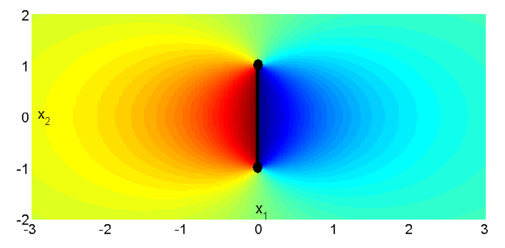
To understand the physics of (41), we compare the expression between braces to the expectation value of the Polyakov loop correlator , where the two circles wind around the thermal direction. This correlator gives us information about the potential between two infinitely heavy electric probes. To understand the geometry of the loop , we start by considering a rectangular loop that lies on the plane at . The Polyakov loop correlator is a gauge invariant quantity and in principle one can choose the loop to lie on any plane. However, our many-body Hamiltonian (37) is written in terms of the potential which is a gauge-dependent quantity. Therefore, given the gauge (17), one is forced to place the loop in a specific plane (the plane in our case) in order to hide the Dirac string singularities, as we will demonstrate shortly. The loop extends from (the position of the first probe) to (the position of the second probe), and from to . Because the coordinate has the geometry of a circle, we identify the edges and keeping in mind that we are working in the limit . This results in the loop or for short. Then, using Gauss’s theorem, we obtain , where is the magnetic flux through the cylinder wrapping the thermal direction. This geometry is illustrated in Figure (2). The magnetic field due to magnetic charge density is . Hence, the quantity can be written as , where is the magnetic flux through the surface due to a unit magnetic charge located at . The computation of is carried out in Appendix A to find , which is the quantity that appears in (41). Further, by studying the properties of , we find that the appropriate jump in the flux happens when the two electric probes are positioned along the -axis. This is illustrated in Figure (3) which explains why we placed the loop in the plane. The only place where we can allow for a discontinuity in the flux is across the line connecting the two charges. Had we placed the charges along any other axis, the flux would be discontinuous across arbitrary places.
In order to further simplify our analysis, we use a mean-field approach to replace the monopole-monopole Coulomb interaction (the first line in (37)) with an effective description. In this approach, one does not have to account for the individual behavior of each monopole. Rather, we use the fact that the monopole-instantons form a plasma of positive and negative charges to deduce the form of the collective behavior of the monopole density correlation function , where the brackets denote a statistical average. We explicitly compute this quantity in the next section assuming the fluctuations of the density to follow a Gaussian distribution, i.e. . Therefore, one can replace the full partition function (35), which involves a sum over an arbitrary number of monopole-instantons, with the ”effective” partition function
| (42) |
where
| (43) |
The subscript in denotes the effective partition function of the ”electric” probes. This is to distinguish it from the effective partition function of the ”magnetic” probes that we consider in the next section.
Since the statistical average in (43) is performed over Gaussian fluctuations, we have for any odd correlator . On the other hand, one can use the Wick’s theorem to write the even correlators in terms of the lowest moment :
| (44) |
Substituting (44) into (42), we finally obtain
| (45) |
To calculate the correlator , it is more appropriate to go to the Fourier basis. The Fourier decomposition of and is given by
| (46) |
where are the Matsubara frequencies. 88 8 In general, given the periodic function , the Fourier transform reads (47) while the inverse Fourier transform is given by (48) The form of the Fourier decomposition of the density-density correlation function, such that depends only on a single momentum , is a consequence of the fact that the monopole-instanton plasma is invariant under spacetime translation. Substituting (46) into we find
Since the external probes are not dynamical, we notice that the expression above has a contribution coming only from the zero Matsubara frequency. The second term in () can be represented diagrammatically as in Figure (4). This expression can also be obtained by performing a perturbative expansion to the expectation value of the Wilson loop, which is presented in Appendix A. Before proceeding to calculate the potential between the external probes in the background of the monopole-instanton plasma, we pause to calculate the correlation function using a mean-field approach.
3.2 The monopole-instanton density-density correlation function: the ’t Hooft loop correlator
The density-density correlation function of the monopole-instanton plasma can be obtained in a similar fashion to what we did in the previous section. In this regard, we introduce two infinitely heavy external magnetic probes with magnetic charges and located respectively at and , where and are the three-dimensional Euclidean position vectors. Calculating the effective potential between these two external probes amounts to the computation of the ’t Hooft magnetic correlator. Since these calculations are performed at , we drop the contribution from the W-bosons. The free action due to the interaction between the two probes reads
| (50) |
The interaction Hamiltonian of the monopole gas in the presence of the external monopole-instanton impurities is
| (51) |
As we did before, we omit the first term in (51) and replace it by an effective description. In this description we encode the effect of the monopole-instanton plasma in the density-density correlation function. Again, we assume that the fluctuations in the density function follow a Gaussian distribution, i.e. . By repeating the same steps that led us from (37) to () we obtain the partition function that describes the ”effective” monopole-instanton plasma in the presence of the external magnetic probes:
| (52) | |||||
where the subscript in denotes the effective ”magnetic” partition function. According to (48), the potential is given by
| (53) | |||||
The quantity between brackets in (52) can be recognized as an effective dielectric constant for the monopole-instanton plasma:
| (54) |
This dielectric constant can be modeled using a mean-field approach. The physics of the three-dimensional monopole-instanton plasma is that the Coulomb interactions are screened. Thus, the potential between two external probes is given by
| (55) |
where is the mass gap or equivalently the inverse Debye screening length of the monopole plasma. 99 9 Contrasting the form of the density-density correlation obtained from the mean-field approach with the same quantity obtained using the Polyakov calculations (reviewed in Appendix A), one can read the relation between the mass gap and the monopole fugacity (56) This potential can be written as , where . Using the definition (54) we obtain
| (57) |
3.3 Calculations of the confinement potential
Having calculated the density-density correlator, the final step before applying the master formula () is to calculate the Fourier transform of :
| (58) | |||||
where is given by (40). The remaining two-dimensional integral can be done by using methods of generalized Fourier transform. Alternatively, we proceed by recalling the discussion after (40). There, we argued that there is a discontinuity in the magnetic flux as we cross the -axis, while the flux is continuous along the -axis. Then, we use the two-dimensional duality between the angle and logarithm , where . Since is continuous along the -axis, we demand that . The Fourier transform of the previous relation is . Then, we obtain
| (59) |
Finally, we are in a position to calculate the potential between two external probes. Putting everything together and remembering that the electric probes are separated a distance along the -axis, we find
| (60) | |||||
The integral can be obtained in a closed form in terms of the Meijer- function [27], and the total potential between the electric probes read
This is one of the main results in the present work. For , we use the asymptotic expansion
to find that the logarithms cancel at large distances
| (67) |
where
| (68) |
is the string tension calculated using the mean-field approach. The behavior of and its derivative (the electric field) is depicted in Figure (1). Interestingly enough, the smooth transition from logarithmic to linear potential is an indication of the conservation of the electric flux. Comparing to the string tension calculated originally in [5], , we find that the mean-field value is off by a factor of . Such discrepancy is attributed to strong coupling physics that is not taken care of in the mean-field approach. Another method to calculate is presented in Appendix A.
4 The finite temperature effects
In the previous section, we performed our calculations strictly at zero temperature. In this section, we consider the finite temperature effects. Unlike the zero temperature case, the W-bosons are now excited and will modify the confinement picture. Their effect is well pronounced near the confinement-deconfinement transition region where they play a prominent role. In order to take these effects into consideration, one needs a systematic approach to start from the relativistic partition function (22) and integrate out the W-bosons. This is achieved using a heat kernel expansion technique that takes into account the presence of the thermal holonomy. One can also obtain the same results starting from the non-relativistic partition function (31). Such calculations work as a non-trivial check on the many-body approach described in the previous section.
4.1 Integrating out the heavy fields: the effective action
Our starting point is the relativistic partition function (22). This partition function encodes all information about the system at all temperatures. Basically, it includes a path sum over the monopole-instanton gas as well as the fluctuations of the electromagnetic , W-boson , Higgs , Goldston boson , and the ghost fields. It is important to emphasize again, as mentioned in section (2), that the electromagnetic field includes both the photon and monopole-instanton contribution ; thus . The fields , , and are massive with mass , while the mass of the Higgs field depends on the quartic coupling constant . In the following, we are interested in the system behavior at temperatures lower than the W-boson mass, . Hence, one can integrate out the fields , , and . Since the Higgs field is massive, it is short ranged and does not participate in the dynamics. Therefore, we can equally well integrate it out or just leave it aside.
Integrating out the heavy fields , , , and , and ignoring the non-quadratic terms in (15), which contribute only to higher order effects, we obtain
| (69) | |||||
where . We leave the dimension of the spacetime unspecified and equal to setting at the end of calculations. Now, we use the identity to write the partition function as
| (70) |
and the effective action is given by
| (71) |
where , , and we neglected the determinant over the Higgs field since it can only modify the short range physics. 1010 10 The effect of a finite Higgs mass on the deconfinement transition was considered in [28]. The trace Tr denotes the trace over both spacetime and Lorentz (Euclidean) indices. Thus we have , where tr denotes the trace over the Lorentz indices. At this stage, it is useful to use the zeta function regularization technique to express the trace s in terms of the diagonal matrix elements of the heat kernel :
| (72) |
Now, we are in a position to calculate the effective action (70) upon compactifying one of the dimensions over a thermal circle . In fact, one just needs to calculate the heat kernels over the manifold . This will be achieved in the next section.
4.2 The heat kernel expansion
The heat kernel expansion methods is a systematic way to carry out a series expansion of the operators in powers of the parameter using only gauge invariant quantities as expansion coefficients. However, the expansion is local and hence is insensitive to the global structure of the background manifold. Therefore, one normally would expect the expansion coefficients to be functions of the local gauge invariant quantity . Such an expansion can easily overlook non-trivial global gauge invariant structures on the background manifold. This is particularly clear in the case of gauge theories formulated on , where the manifold admits a gauge holonomy or the Polyakov loop around the thermal circle:
| (73) |
If we choose a gauge in which is time independent, then we find . Thus, the Polyakov loop is basically the exponent of the zero frequency component of the gauge field along the thermal circle, which constitutes a global gauge invariant quantity. Therefore, one needs to carry out a systematic expansion in powers of with expansion coefficients as functions of the two gauge invariant quantities and , keeping in mind that the Lorentz invariance of the theory is explicitly broken due to the presence of the heat path. Such a systematic approach was developed in [29, 30].
Given a massless Klein-Gordon operator of the form , where is a local function of , the authors in [29, 30] showed that
| (74) |
where denotes the trace over the Lorentz indices. 1111 11 Also, see [31] for the heat kernel expansion for spacetimes with topology . Unlike the case of non-compact spaces, where only integer powers of appear in the expansion, half-integer powers of are also allowed in the present case. The coefficients are given, up to the second power of , by
| (75) |
and the electric field is defined as . 1212 12 Notice that the first non-zero half-integer coefficient is which we do not consider here; see [30]. The functions are periodic functions of the Polyakov loop
| (76) |
where are the Matsubara frequencies. Notice that the potential along the circle as well as the one-loop induced field strength have contributions from both the photon and monopole fields, as was stressed above, i.e. , and .
Since our Klien-Gordon operators , , and are massive, with mass , we need to modify the coefficients in (75). This can be done either by resumming the series in (74) or slightly modifying the derivation in [30] that leads to (75). Simply, noticing that , the part in the coefficients is resummed to give . Then, the heat kernel expansion is given by the modified expression
| (77) |
The coefficients are given by (75) after making the replacement , and we have for (the Lorentz structure is implicitly understood), and for both and .
Taking the trace over the Lorentz indices, we obtain up to the second power in in the heat kernel expansion
| (78) | |||||
where we have used which proves to be useful in simplifying the sums over the Matsubara frequencies. These sums are evaluated in Appendix B. The expressions for the different terms are given by (125), (126), and (127), where we also give the leading-order behavior in the limit . Collecting everything and setting , we find that the effective action in the limit reads
The term is a temperature-independent one-loop correction to the free Lagrangian. Hence, we defined the effective coupling constant as .
Now, a few remarks are in order:
- 1.
The terms and multiply the exponentially small factor . Therefore, both terms can be neglected compared to the kinetic term . This is unlike the term which is responsible for highly non-trivial dynamics. As we show in the following section, the partition function (70) with the effective action
(80) represents a double Coulomb gas of electrically (W-bosons) and magnetically (monopole-instantons) charged particles. Each type of particles carry a positive or negative unit charge and interact via a long-range potential, while the electric and magnetic charges have the Aharonov-Bohm phase interaction. It is the term in (80) that is responsible for the later type of interaction.
- 2.
It is important to emphasize that the effective action (80) is a gauge-invariant quantity. This is obvious since both and are gauge-invariants.
- 3.
The effective action (80) description is valid for all temperatures in the range .
- 4.
The term is the leading order contribution coming from the full calculations of the effective action as presented in Appendix B. Higher order corrections will generally have the form , where is a polynomial in . Such terms describe complex molecules of W-bosons with higher mass and charge and in principle can be added to the Coulomb gas. However, such molecules have highly suppressed dynamics thanks to the Boltzmann suppression factor for all molecules with , and hence we ignore them in the following analysis.
4.3 The double Coulomb gas
The first step in dealing with the partition function (70) is to manipulate the term . Recalling that , as well as the definitions (19) and (73), and taking into account the fact that our theory is formulated on a thermal circle (hence the monopole-instanton field is the result of the sum of an infinite number of images along the circle), we obtain
| (81) | |||||
where we have used the trick in (39), and the angle is defined in (40). Then, we use to expand the terms as follows
| (82) |
where . We apply the expansion (82) to the term to find that the partition function (70) reads
where is the W-boson fugacity. 1313 13 This fugacity can also be obtained by integrating the Boltzmann distribution of a single W-boson , where , over the particle momenta: (84) where is the spin degeneracy factor of the W-bosons. Since the expansion in goes hand in hand with the expansion in the W-boson fugacity , it is natural to interpret as the positions of these W-bosons and as their charges. In fact, as we show below, it turns out that this is the correct interpretation of and .
Next, we turn to the calculations of the path integral over . This path integral is plagued by the presence of monopole-instantons. The reason is that the potential , which naturally describes the force mediation between W-bosons, should also describe the force between monopole-instantons. However, as we mentioned in section 2, such a description is only possible on the expense of allowing Dirac-like singularities to appear in the gauge potential which can lead to inconsistencies. In other words, one has to exercise caution while carrying out the path integral over the field which, in our case, is used to describe both electric and magnetic forces. In the absence of magnetic objects, the gauge potential is a genuine tool to describe the electric force between electrically charged particles. We call this the abelian electric group. On the other hand, in the presence of magnetic charges, and absence of any electric objects, one needs to go to a dual description to avoid the Dirac singularities that appear when using the electric . The dual fields are invariant under a dual that is known as the abelian magnetic group. The dual description can be performed by introducing a Lagrange multiplier field as to the action to enforce the Bianchi identity everywhere except at the position of the magnetic charges. Then, we vary with respect to to find and substitute back into . The result is the action in terms of the dual photon field . This dual description was used in the original work of Polyakov [5] to account for the monopole-instanton plasma.
Fortunately enough, there exists a duality transformation prescription that enables us to perform the integral over without having to run into contradictions even in the presence of both electric and magnetic charges [32]. In this prescription, one enlarges the electric gauge symmetry to . It is this extra gauge redundancy that enables us to perform the path integral over both electric and magnetic objects without running into difficulties. 1414 14 I am grateful to Erich Poppitz for elucidating this method. As a warm up exercise, we first show that the path integral is equivalent to the path integral where
| (85) |
This Lagrangian is invariant under two different s: the first is given by and , while the second is . Setting (or in other words, using the unitary gauage), and varying with respect to we find that the equation of motion of reads . Then, substituting back into we obtain which proves the equivalence of the above mentioned path integrals to each other.
Now, we come to the path integral over in (). According to the duality transformation prescription, we trade the Lagrangian (85) for the term which results from expanding the square in the last line in (). Thus, we express the path integral over as a double path integral over and the additional auxiliary field :
| (86) |
where
| (87) | |||||
Varying with respect to and substituting the resulting equation of motion back into (87), we obtain the final expression of the grand partition function (the details of the procedure are presented in Appendix C):
The Green’s function satisfies , where the Laplacian is defined over . The Green’s function is given by
| (89) |
The partition function () describes a grand-canonical distribution of a three-dimensional double Coulomb gas of W-bosons and monopole-instantons at finite temperature . The W-bosons are physical particles and therefore they sweep world-lines as time elapses. These bosons interact logarithmically at all temperatures which is the expected behavior for particles in D. On the contrary, the monopole-instantons are pseudo-particles; they represent localized events which interact via (89). In addition, the W-bosons and monopole-instantons interact via the Aharonov-Bohm phase . A picture of this gas is depicted in Figure (5).
4.4 Obtaining the Coulomb gas from the non-relativistic partition function
The non-relativistic partition function (31), along with the Lagrangian (32), is readily in the form of a Coulomb gas. Comparing (31) with (), we see the expected form of interaction between the same species: the logarithmic potential between the W-bosons as well as the interaction between the monopole-instantons. What remains to be shown is the Aharonov-Bohm phase interaction between the W-bosons and monopole-instantons. To show that such term arises naturally from (31) we proceed as follows. First, we notice that the term , which accompanies the kinetic factor , is suppressed by the W-boson mass compared to the term , and hence we ignore it. Also, we leave aside the Coulomb interaction terms in (32), which are left intact in our present treatment. Then, we have for the remaining part of the partition function
| (90) |
where
Using (25) and (27) to express the operators and in terms of the defining Dirac-delta functions, and using (17) to perform the integral over , noticing that , we find
| (92) | |||||
Since the action (92) is quadratic in the fields and , we can perform the path integral exactly to obtain
| (93) | |||||
where is the spin degeneracy factor of the W-boson which is in D. Therefore, the partition function (90) can be casted in the form , where
| (94) |
The expression of is in the form of the non-relativistic limit of (124). Following the same procedure that led from (124) to (125), we find
| (95) |
Finally, using (82) and restoring the Coulomb interaction terms, we recover the partition function of the double Coulomb gas (), apart from the trivial renormalization . In fact, these calculations are a non-trivial check on our many-body formulation presented in Section 3.
4.5 The two-dimensional Coulomb gas and deconfinement transition
As we mentioned above, the partition function () encodes all information about the double Coulomb gas for temperatures in the range . At zero temperature, the monopole-insatntons proliferate and form a plasma of magnetic charges. This works as a dual Meissner effect which screens the magnetic field lines. The monopole-instanton fugacity is , where here and in the following analysis we omit dimensionfull pre-exponential factors and work in the BPS limit. Thus, the average distance between two monopoles in the plasma is . Then, two external electric probes separated a distance experience a linear confining potential , where is the string tension. This continues to be the case as we slightly increase the temperature of the gauge theory. However, at any non-zero temperature, the W-bosons will start to proliferate according to the Boltzmann distribution .
At low temperatures, the W-bosons will form electrically neutral dipoles which screen the electric flux lines of the external probes resulting in a decrease of the string tension. The average size of the - dipoles can be determined using simple classical statistical arguments. First, we model the potential between the and constituents of the dipole by
| (96) |
A better model would use the potential (3.3). However, this adds unnecessary complications to our problem. The average size of the - molecule is given by
| (97) |
where is the deconfinement temperature, as we argue below, and is a UV cutoff. At low temperatures, , we expand about to find
| (98) |
This means that at low temperatures, the average size of the W molecules is determined by the UV cutoff of the theory, , where the logarithmic interaction dominates over the linear confinement potential. At temperatures , the average size of the molecules can be obtained by expanding (97) about
| (99) |
Hence, at temperatures , the linear potential dominates over the logarithmic interaction and we can visualize the gas as neutral molecules of W-bosons bound due to the existence of long flux tubes or in other words strings. This behavior is illustrated in Figure 6.
On the other hand, the number density of the W-bosons is . Hence, the average distance between two W-bosons is . Thus, we have for all which justifies the above picture of having a dilute gas of W-molecules. Near the transition temperature from below , the separation between the W-bosons inside the molecules becomes comparable to , and therefore we basically have a gas of free W-bosons. This justifies that is the critical deconfinement temperature.
Such picture can be confirmed more rigorously by studying the phase transition of the double Coulomb gas in (). At temperatures much higher than the inverse distance between monopole-instantons, , yet much lower than the deconfinement transition temperature, , the effective interaction between two monopoles is two-dimensional, and one has for the Green’s function that appears in () . Thus, the double Coulomb gas () becomes essentially two-dimensional. Such a two-dimensional double Coulomb gas was studied previously in [17]. This was done by mapping the gas to a dual-sine-Gordon model. Indeed, it was found that a second-order phase transition takes place at . We do not elaborate further on the nature of the transition, and we refer the reader to the original literature for more details.
5 Conclusion and future directions
In this work, we have studied several issues of the confinement problem in the Georgi-Glashow model in D. The aim of our study was two-fold. First, we worked out a many-body description of the effective degrees of freedom, namely W-bosons and monopole-instantons, for temperatures in the range , where the W-bosons are non-relativistic. In this approach, we wrote down a partition function for the W-bosons in the background of an arbitrary number of monopole-instantons. This partition function, with the aid of a mean-field approximation, enabled us to find an explicit expression for the potential between two external electric probes at all distances.
Then, we used a systematic method to integrate out the W-bosons at finite temperatures. We started with the relativistic partition function in the background of the instantons field and applied a heat kernel expansion technique that takes into account the existence of a non-trivial thermal holonomy. We found that the partition function describes a three-dimensional two-component Coulomb gas; these are W-bosons and Monopole-instantons. The W-bosons interact logarithmically, while the monopoles interact via the potential , where is the Green’s function of the Laplacian operator on and is the thermal circle. In addition, there is the Aharonov-Bohm phase interaction between the W-bosons and monopole-instantons. Further, we used the finite temperature many-body partition function to arrive to the same picture, which works as an independent check on our many-body methods. For temperatures much larger than the inverse distance between two neighboring monopoles, the Coulomb gas becomes two-dimensional and we recover the previous result of [17].
The Georgi-Glashow model has been an important testing ground for the problem of confinement. In the following, we consider a few venues where our methods can be applied:
- 1.
- 2.
Our many-body approach can be used to study the non-equilibrium phenomena in the Gerorgi-Glashow model, see e.g. [35]. This can shed light on the nature of Yang-Mills in the non-equilibrium state. Recently, a tremendous effort has been made to calculate various kinetic coefficients, e.g. shear viscosity, which is important to understand the quark-gluon state of matter.
- 3.
One way of understanding the the color confinement mechanism in -D pure Yang-Mills theory is through the use of abelian monopoles, see e.g. [36, 37]. Moreover, it has been shown that such monopoles can play a prominent role in understanding the deconfinement phase transition in this theory [38]. It will be interesting to use a many-body approach to tackle this problem along the same lines presented in the present work.
- 4.
An important class of theories is Yang-Mills on , where is a spatial circle. These theories abelianize either by adding deformations [39], or by adding adjoint fermions with periodic boundary conditions along the spatial circle [40]. Integrating out the heavy Kaluza-Klein tower results in an effective potential for the gauge-component along the direction, which can be thought of as a compact adjoint scalar. This reduces the Yang-Mills to a Georgi-Glashow model, possibly with adjoint fermions. In [41], it was shown that Yang-Mills with adjoint fermions on , near the confinement-deconfinement transition region, can be mapped to two-dimensional ”affine” XY spin models. These spin models can be studied analytically or numerically, by means of Monte Carlo simulations [42], which can shed light on the nature of the deconfinement transition in Yang-Mills in D. The mapping between the gauge theories and spin models was possible by showing that the partition function of both systems is that of a two-dimensional two-component Coulomb gas. Regarding (1) above, our methods provide a systematic way of deriving the Coulomb gas partition function even in the presence of an additional scalar or fermion fields, which can arise in this class of theories.
Acknowledgment
I would like to thank Erich Poppitz for collaboration at the early stages of this project, for many enlightening discussions and comments on the manuscript. I would also like to thank Mithat Ünsal for valuable comments on the manuscript. I am also thankful to Yulia Smirnova for editing the manuscript. This work has been supported by NSERC Discovery Grant of Canada.
Appendix A The Wilson loop calculations
In this section, we derive the result (68) by performing a perturbative treatment to the expectation value of the Wilson loop. Before performing these calculations, we first review the steps that lead to the exact result of the string tension that was obtained by Polyakov [5]. Then, we redo the Polyakov’s calculations using a Gaussian approximation. This introduces an error in the value of the string tension due to the neglection of the non-Gaussianities. This value of the string tension coincides with the value we obtained in Section 3 using the many-body approach.
A.1 The exact Polyakov calculations
The exact partition function of the monopole-instanton gas was obtained by Polyakov in a seminal paper [5]:
| (100) |
where is the dual photon field, and is its mass. In order to find the string tension, we calculate the expectation value of the Wilson loop:
| (101) |
where and are respectively a closed loop and the surface enclosed by it, and the equality in the above equation is a result of using the Gauss’s theorem. The magnetic field is sourced by the monopole-instantons:
| (102) |
Hence, the Wilson loop can be written as
| (103) |
where
| (104) |
The quantity is the magnetic flux through the surface due to a unit magnetic charge located at position in the Euclidean spacetime. Including the Wilson loop into (100), one finds 1515 15 We refer the reader to the original literature [5] for details.
| (105) |
The dominant contribution to comes from the classical solution to the effective action. Thus, one extremizes to obtain the sine-Gordon equation
| (106) |
We can choose the loop to be an infinite loop that lies on the plane. Hence, the above equation reduces to
| (107) |
where we have used . Solving for and substituting back into , one obtains the string tension
| (108) |
A.2 The Guassian approximation to the Polyakov model
In this section, we redo the Polyakov calculations using the Gaussian approximation (or mean-field approximation), i.e. taking . In this case, the expectation value of the Wilson loop is
| (109) |
The corresponding domain-wall equation (107) reduces to
| (110) |
The solution to this equation is given by
| (111) |
where is the sign function. Substituting back into , we find
| (112) |
This coincides exactly with (68) obtained using the many-body approach. Comparing (112) with the exact result (108), we find that the mean-field calculations, , are off by a factor of .
A.3 The perturbative treatment of the Wilson loop
In this section, we perform a perturbative treatment to the expectation value of the Wilson loop. By doing that, we recover the second term of (), which works as an alternative derivation of the potential between two external probes. We start from (103), assume that the monopole-instanton density follows a Gaussian distribution, i.e. , and expand in to find
| (113) |
where
and we used the fact that the correlators of an odd number of density operators vanish identically in the Gaussian approximation. Taking the Fourier transform, we obtain
| (114) |
Let us notice that expanding in is a legitimate thing to do since the monopole density is assumed to be low. This is a prerequisite for the validity of the dilute gas approximation that we assume throughout this work.
As we mentioned above, we assume that the density-density correlation function can be obtained within the Gaussian approximation. The function can be obtained from (100) by taking the functional derivative of (103) with respect to and . Then, using the Gaussian approximation (109), and taking the functional derivative in the Fourier space, we find
| (115) |
Similarly, the -point density correlator can be calculated by taking the -th functional derivative with respect to some external current source to find 1616 16 We hasten to warn the reader that the density-density correlation function given in [5] is not correct.
| (116) |
For example, the four-point function reads
| (117) | |||||
Next, we compute as given from (104), where the surface is to be taken in the plane setting . In the zero temperature case, we take a loop that extends from to and from to . Alternatively, we can perform our calculations at a finite temperature and then we take . By doing that, we compactify the direction over a circle of radius , and hence we sum over an infinite tower of modes along the direction. In this case, the surface is a cylinder of radius that extends from to , see Figure (2). Thus, we have
| (118) | |||||
Using the definition (40), we can write as
| (119) |
where , and is a unit vector in the -direction. In the limit we find a discontinuity in the value of as we cross the -axis. Hence, , in addition of being the magnetic flux due to a unit magnetic charge, it is also the solid angle seen by a monopole-instanton located at the Euclidean point . Now, we take the Fourier transform of to obtain
| (120) |
where
| (121) |
We note that the choice of the symbol to denote the Fourier transform of is not arbitrary. Recalling (119) and (58), we see that is just the Fourier transform of the angle .
Appendix B Sums and integrals
In this appendix, we perform the Matsubara sums and integrals in (78). First, we consider the function . Integrating over , and taking the derivative with respect to at , we obtain
| (124) |
Since this sum is divergent, we first differentiate the above expression with respect to and perform the sum. Then, we integrate over to get a function that behaves as at . To regularize the integral, we subtract the same form of the integral evaluated at . Then, we find
| (125) | |||||
Next, we turn to the term . Performing the integral over , taking the derivative with respect to at , performing the integral over , and then summing over the Matsubara frequencies, we find
| (126) |
Finally, by repeating the same steps we followed to calculate , we obtain for
| (127) |
Appendix C Performing the path integral using the duality transformation prescription
In this appendix, we work out the details that lead us to the partition function () starting from the auxiliary action
| (128) | |||||
Varying (128) with respect to , we obtain
| (129) |
The solution to the equation of motion (129) is given by
| (130) |
where . The vector field can be decomposed into curl-free and divergence-free parts
| (131) |
where . Substituting (130) and (131) into (129), we find that the parts drop out, while the equation of reads
| (132) |
where the Laplacian is defined on . At this stage, let us define the Green’s function , which satisfies
| (133) |
The solution to (133) on is
| (134) |
Then, the solution is given by
| (135) | |||||
Now, the solution reads
| (136) |
where
| (137) |
Next, we substitute into (128) and use integration by parts to obtain
| (138) |
The term is obviously zero due to the anti-symmetry of , while . Next, we turn to the calculations of the other terms (138). The monopole-instanton field is
| (139) |
where the superscript , as usual, denotes the periodicity along , which can be enforced by summing an infinite number of images along the circle. Then we have
| (140) | |||||
which is zero under symmetric integration. Then, the term is
| (141) | |||||
which is the Coulomb potential between W-bosons. Finally, varying (138) with respect to , we obtain
| (142) |
which is solved by
| (143) |
Collecting everything and substituting in (138), we find
| (144) |
Thus, the full partition function reads
which is valid in the range .
References
- [1] C. -N. Yang and R. L. Mills, “Conservation of Isotopic Spin and Isotopic Gauge Invariance,” Phys. Rev. 96, 191 (1954).
- [2] J. Greensite, “An introduction to the confinement problem,” Lect. Notes Phys. 821, 1 (2011).
- [3] M. Shifman and M. Unsal, “Confinement in Yang-Mills: Elements of a Big Picture,” Nucl. Phys. Proc. Suppl. 186, 235 (2009) [arXiv:0810.3861 [hep-th]].
- [4] A. M. Polyakov, “Compact Gauge Fields and the Infrared Catastrophe,” Phys. Lett. B 59, 82 (1975).
- [5] A. M. Polyakov, “Quark Confinement and Topology of Gauge Groups,” Nucl. Phys. B 120, 429 (1977).
- [6] H. Georgi and S. L. Glashow, “Unified weak and electromagnetic interactions without neutral currents,” Phys. Rev. Lett. 28, 1494 (1972).
- [7] N. J. Snyderman, “The Physics Of Dual Vortices And Static Baryons In (2+1)-dimensions,” Nucl. Phys. B 218, 381 (1983).
- [8] G. ’t Hooft, “Magnetic Monopoles in Unified Gauge Theories,” Nucl. Phys. B 79, 276 (1974).
- [9] A. M. Polyakov, “Particle Spectrum in the Quantum Field Theory,” JETP Lett. 20, 194 (1974) [Pisma Zh. Eksp. Teor. Fiz. 20, 430 (1974)].
- [10] G. ’t Hooft, “Gauge theories with unified weak, electromagnetic, and strong interactions,” In *t’Hooft, G. (ed.): Under the spell of the gauge principle* 174-203, and In *Palermo 1975, Proceedings, High energy physics, vol. 2* 1225-1249. (708497)
- [11] S. Mandelstam, “Vortices And Quark Confinement In Nonabelian Gauge Theories,” Phys. Lett. B 53, 476 (1975).
- [12] A. A. Abrikosov, “On the Magnetic properties of superconductors of the second group,” Sov. Phys. JETP 5, 1174 (1957) [Zh. Eksp. Teor. Fiz. 32, 1442 (1957)].
- [13] N. Seiberg and E. Witten, “Electric - magnetic duality, monopole condensation, and confinement in N=2 supersymmetric Yang-Mills theory,” Nucl. Phys. B 426, 19 (1994) [Erratum-ibid. B 430, 485 (1994)] [hep-th/9407087].
- [14] N. Seiberg and E. Witten, “Monopoles, duality and chiral symmetry breaking in N=2 supersymmetric QCD,” Nucl. Phys. B 431, 484 (1994) [hep-th/9408099].
- [15] D. J. Gross, R. D. Pisarski and L. G. Yaffe, “QCD and Instantons at Finite Temperature,” Rev. Mod. Phys. 53, 43 (1981).
- [16] N. O. Agasian and K. Zarembo, “Phase structure and nonperturbative states in three-dimensional adjoint Higgs model,” Phys. Rev. D 57, 2475 (1998) [hep-th/9708030].
- [17] G. V. Dunne, I. I. Kogan, A. Kovner and B. Tekin, “Deconfining phase transition in (2+1)-dimensions: The Georgi-Glashow model,” JHEP 0101, 032 (2001) [hep-th/0010201].
- [18] I. I. Kogan and A. Kovner, “Monopoles, vortices and strings: Confinement and deconfinement in (2+1)-dimensions at weak coupling,” In *Shifman, N. (ed.): At the frontier of particle physics. Vol. 4* 2335-2407 [hep-th/0205026].
- [19] D. Antonov and M. C. Diamantini, “3D Georgi-Glashow model and confining strings at zero and finite temperatures,” In *Shifman, M. (ed.) et al.: From fields to strings, vol. 1* 188-265 [hep-th/0406272].
- [20] M. Shifman, “Advanced topics in quantum field theory: A lecture course,” Cambridge, UK: Univ. Pr. (2012) 622 p
- [21] M. K. Prasad and C. M. Sommerfield, “An Exact Classical Solution for the ’t Hooft Monopole and the Julia-Zee Dyon,” Phys. Rev. Lett. 35, 760 (1975).
- [22] E. B. Bogomolny, “Stability of Classical Solutions,” Sov. J. Nucl. Phys. 24, 449 (1976) [Yad. Fiz. 24, 861 (1976)].
- [23] T. W. Kirkman and C. K. Zachos, “Asymptotic Analysis Of The Monopole Structure,” Phys. Rev. D 24, 999 (1981).
- [24] X. G. Wen, “Quantum field theory of many-body systems: From the origin of sound to an origin of light and electrons,” Oxford, UK: Univ. Pr. (2004) 505 p
- [25] G. D. Mahana, “Many-Particle Physics (Physics of Solids and Liquids),” Springer; Softcover reprint of hardcover 3rd ed. 2000 edition, 785 p
- [26] A. M. Tsvelik, “Quantum Field theory in condensed matter physics,” Cambridge University Press, second edition (2003), 360 p
- [27] H. Bateman, A. Erdelyi, “ Higher Transcendental Functions, Vol. I,” New York: McGrawHill (1953)
- [28] Y. V. Kovchegov and D. T. Son, “Critical temperature of the deconfining phase transition in (2+1)-d Georgi-Glashow model,” JHEP 0301, 050 (2003) [hep-th/0212230].
- [29] E. Megias, E. Ruiz Arriola and L. L. Salcedo, “The Polyakov loop and the heat kernel expansion at finite temperature,” Phys. Lett. B 563, 173 (2003) [hep-th/0212237].
- [30] E. Megias, E. Ruiz Arriola and L. L. Salcedo, “The Thermal heat kernel expansion and the one loop effective action of QCD at finite temperature,” Phys. Rev. D 69, 116003 (2004) [hep-ph/0312133].
- [31] F. J. Moral-Gamez and L. L. Salcedo, “Derivative expansion of the heat kernel at finite temperature,” Phys. Rev. D 85, 045019 (2012) [arXiv:1110.6300 [hep-th]].
- [32] P. Deligne, P. Etingof, D. S. Freed, L. C. Jeffrey, D. Kazhdan, J. W. Morgan, D. R. Morrison and E. Witten, “Quantum fields and strings: A course for mathematicians. Vol. 1” Providence, USA: AMS (1999) 1-1501
- [33] G. V. Dunne, A. Kovner and S. M. Nishigaki, “Fundamental matter and the deconfining phase transition in (2+1)-D,” Phys. Lett. B 544, 215 (2002) [hep-th/0207049].
- [34] D. Antonov and A. Kovner, “SUSY 3-D Georgi-Glashow model at finite temperature,” Phys. Lett. B 563, 203 (2003) [hep-th/0303184].
- [35] J. Rammer, “Quantum field theory of non-equilibrium states,” Cambridge University Press; Reissue edition (March 3, 2011)
- [36] D. Diakonov and V. Petrov, “Confining ensemble of dyons,” Phys. Rev. D 76, 056001 (2007) [arXiv:0704.3181 [hep-th]].
- [37] F. Bruckmann, S. Dinter, E. -M. Ilgenfritz, B. Maier, M. Muller-Preussker and M. Wagner, “Confining dyon gas with finite-volume effects under control,” Phys. Rev. D 85, 034502 (2012) [arXiv:1111.3158 [hep-ph]].
- [38] A. D’Alessandro, M. D’Elia and E. V. Shuryak, “Thermal Monopole Condensation and Confinement in finite temperature Yang-Mills Theories,” Phys. Rev. D 81, 094501 (2010) [arXiv:1002.4161 [hep-lat]].
- [39] M. Unsal and L. G. Yaffe, “Center-stabilized Yang-Mills theory: Confinement and large N volume independence,” Phys. Rev. D 78, 065035 (2008) [arXiv:0803.0344 [hep-th]].
- [40] M. Unsal, “Magnetic bion condensation: A New mechanism of confinement and mass gap in four dimensions,” Phys. Rev. D 80, 065001 (2009) [arXiv:0709.3269 [hep-th]].
- [41] M. M. Anber, E. Poppitz and M. Unsal, “2d affine XY-spin model/4d gauge theory duality and deconfinement,” JHEP 1204, 040 (2012) [arXiv:1112.6389 [hep-th]].
- [42] M. M. Anber, S. Collier and E. Poppitz, “The QCD(adj) deconfinement transition via the gauge theory/’affine’ XY-model duality,” JHEP 1301, 126 (2013) [arXiv:1211.2824 [hep-th]].