跳到论文正文
W Papers独立论文阅读器 arXiv:1307.8429 论文正文 计算阅读时间 · 0%
引用这篇论文根据当前论文元数据生成,正式投稿前建议核对。


License: arXiv.org perpetual non-exclusive license
arXiv:1307.8429v3 [math.NA] 14 Nov 2013

The Intersection of Bivariate Orthogonal Polynomials on Triangle Patches

Tom H. Koornwinder ††thanks: Korteweg-de Vries Institute for Mathematics, University of Amsterdam, P.O. Box 94248, 1090 GE Amsterdam, Netherlands, e-mail: T.H.Koornwinder@uva.nl    Stefan A. Sauter ††thanks: Institut für Mathematik, Universität Zürich, Winterthurerstrasse 190, CH-8057 Zürich, Switzerland, e-mail: stas@math.uzh.ch
Abstract

In this paper, the intersection of bivariate orthogonal polynomials on triangle patches will be investigated. The result is interesting by its own but also has important applications in the theory of a posteriori error estimation for finite element discretizations with pp-refinement, i.e., if the local polynomial degree of the test and trial functions is increased to improve the accuracy. A triangle patch is a set of disjoint open triangles whose closed union covers a neighborhood of the common triangle vertex. On each triangle we consider the space of orthogonal polynomials of degree nn with respect to the weight function which is the product of the barycentric coordinates. We show that the intersection of these polynomial spaces is the null space. The analysis requires the derivation of subtle representations of orthogonal polynomials on triangles. Up to four triangles have to be considered to identify that the intersection is trivial.
Keywords: A posteriori error estimation, saturation property, pp-refinement, Jacobi polynomials, orthogonal polynomials on the triangle, intersections of nn-th degree orthogonal polynomial spaces
Mathematics Subject Classification (2010): 65N15, 65N30, 65N50, 33C45, 33C50

1 Introduction

In this paper, we will investigate the intersection of bivariate orthogonal polynomials on triangle patches. This problem arises in the theory of a posteriori error estimation for finite element discretizations of elliptic partial differential equations — in particular if the local polynomial degree of the finite element spaces is increased during the solution process. Before we give the precise mathematical formulation of this problem we will sketch its application in the finite element analysis.

A posteriori error estimation and adaptivity are well established methodologies for the numerical solution of partial differential equations by finite elements (cf. [2], [3], [21], [1], [4], [18], [9], [16], [19], [7]).

Some types of error estimators, for example hierarchical ones (see, e.g., [5], [8], [6]), require explicitly or implicitly the saturation assumption which states that the error on the refined mesh and/or with higher polynomial degree is strictly smaller than the error on the previous mesh/polynomial degree. In the pioneering paper [10] the saturation assumption is proved for the Poisson problem in two spatial dimensions under the assumption that the data oscillations are small. In [16] the convergence of adaptive finite element methods (AFEM) for general (nonsymmetric) second order linear elliptic partial differential equations is proved, where the term “adaptivity” is understood in the sense of adaptive mesh refinement and the polynomial degree stays fixed. The theory in [16] also generalizes the proof of the saturation property to quite general 2nd order elliptic problems and estimates the error on the refined mesh by the error of the coarser mesh plus a data oscillation term.

For the proof of the saturation assumption for pp-refinement, i.e., when the local polynomial degree of the finite element space is increased instead of the mesh being refined, a difficulty arises which is related to a polynomial projection property on triangle patches. Here orthogonal polynomials in two variables on a triangle (see [17], [15], [12]) enter, and the problem just raised is also interesting by its own in that area. By the way, these orthogonal polynomials also have important applications in the field of spectral methods for discretizing partial differential equations and we refer to [13] for further details. In particular, orthogonal polynomials on triangles can be efficiently used for discontinous Galerkin (dG) methods or to discretize boundary integral equation of negative order since no continuity is required across simplex boundaries.

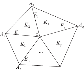
Let us now briefly state the problem which we will solve in this paper. For a two-dimensional domain D⊂ℝ2D\subset\mathbb{R}^{2}, the set of bivariate polynomials of maximal total degree nn is denoted by ℙn​(D)\mathbb{P}_{n}\left(D\right). Put ℙ−1​(D):={0}\mathbb{P}_{-1}(D):=\{0\}. Let z∈ℝ2z\in\mathbb{R}^{2} and let 𝒯:={Ki:1≤i≤q}\mathcal{T}:=\left\{K_{i}:1\leq i\leq q\right\} denote a triangle patch around zz, i.e., 𝒯\mathcal{T} is a set of (open) triangles (cf. Figure 1) which
Refer to caption
Figure 1: Triangle patch 𝒯:={Ki:1≤i≤q}\mathcal{T}:=\left\{K_{i}:1\leq i\leq q\right\} around a point zz. The triangles KiK_{i} and Ki+1K_{i+1} share an edge EiE_{i}. Each triangle KiK_{i} has zz as a vertex while its other vertices are denoted by Ai−1A_{i-1} and AiA_{i}.
  • •

    are pairwise disjoint,

  • •

    have zz as a common vertex.

  • •

    For all 1≤i≤q1\leq i\leq q, the triangles11 1 We use here the convention K0:=KqK_{0}:=K_{q} and Kq+1:=K1K_{q+1}:=K_{1} and analogously for the vertices AiA_{i} and the edges EiE_{i}. Clearly q≥3q\geq 3 holds. KiK_{i} and Ki+1K_{i+1} have one common edge, denoted by EiE_{i}, which connects the common vertices zz and AiA_{i} of KiK_{i} and Ki+1K_{i+1}.

Thus

Ki=convo⁡(z,Ai−1,Ai),K_{i}=\operatorname*{conv^{o}}(z,A_{i-1},A_{i}), (1.1)

where conv denotes the convex hull of the given points and convo\operatorname*{conv^{o}} the open interior of this convex hull.

Let Ω:=int(∪i=1qKi¯)\Omega:=\operatorname*{int}\left(\cup_{i=1}^{q}\overline{K_{i}}\,\right) and let 𝔖:=Ω∩(∪∂i=1q⁡Ki)\mathfrak{S}:=\Omega\cap\left(\cup_{i=1}^{q}\partial K_{i}\right) denote the inner mesh skeleton. We denote by ℙn​(𝒯)\mathbb{P}_{n}\left(\mathcal{T}\right) the space of piecewise polynomials, i.e.,

ℙn(𝒯):={f:Ω\𝔖→ℝ∣∀i∈{1,…,q}f|Ki∈ℙn(Ki)}.\mathbb{P}_{n}\left(\mathcal{T}\right):=\left\{f:\Omega\backslash\mathfrak{S}\rightarrow\mathbb{R}\mid\forall i\in\{1,\ldots,q\}\;\;f\big|_{K_{i}}\in\mathbb{P}_{n}\left(K_{i}\right)\right\}.

We consider ℙn​(Ω)\mathbb{P}_{n}(\Omega) as a linear subspace of ℙn​(𝒯)\mathbb{P}_{n}(\mathcal{T}) by its natural embedding.

For i=1,…,qi=1,\ldots,q define a weight function ωi:=ai​bi​ci\omega_{i}:=a_{i}b_{i}c_{i} on KiK_{i}, where ai,bi,cia_{i},b_{i},c_{i} are affine linear functions which vanish on the respective edges of KiK_{i}. Thus ωi\omega_{i} is the product of the barycentric coordinates in KiK_{i} or, in other terms, a cubic bubble function which is positive on KiK_{i}. We define the inner product (⋅,⋅)𝒯\left(\cdot,\cdot\right)_{\mathcal{T}} on 𝒯\mathcal{T} by

(u,v)𝒯:=∑i=1q(u,v)Ki,\left(u,v\right)_{\mathcal{T}}:=\sum_{i=1}^{q}(u,v)_{K_{i}}, (1.2)

where

(u,v)Ki:=∫Kiu⁡(x,y)​v​(x,y)​ωi​(x,y)​𝑑x​𝑑y.(u,v)_{K_{i}}:=\int_{K_{i}}u(x,y)\,v(x,y)\,\omega_{i}(x,y)\,dx\,dy. (1.3)

Denote by ℙn−1⟂​(Ki)\mathbb{P}_{n-1}^{\perp}(K_{i}) the orthoplement of ℙn−1​(Ki)\mathbb{P}_{n-1}(K_{i}) in ℙn​(Ki)\mathbb{P}_{n}(K_{i}) with respect to the inner product (1.3). Let Πn𝒯:ℙn​(Ω)→ℙn−1​(𝒯)\Pi_{n}^{\mathcal{T}}\colon\mathbb{P}_{n}(\Omega)\to\mathbb{P}_{n-1}(\mathcal{T}) denote the restriction to ℙn​(Ω)\mathbb{P}_{n}(\Omega) of the orthogonal projection of ℙn​(𝒯)\mathbb{P}_{n}(\mathcal{T}) onto ℙn−1​(𝒯)\mathbb{P}_{n-1}(\mathcal{T}) with respect to the inner product (1.2).

Theorem 1.1

Let n≥1n\geq 1. Then the following three statements are equivalent and each of them holds.
(a) If u∈ℙn​(Ω)u\in\mathbb{P}_{n}(\Omega) and (u,w)𝒯=0(u,w)_{\mathcal{T}}=0 for all w∈ℙn−1​(𝒯)w\in\mathbb{P}_{n-1}(\mathcal{T}) then u=0u=0.
(b) ⋂i=1,…,qℙn−1⟂​(Ki)={0}\displaystyle\bigcap_{i=1,\ldots,q}\mathbb{P}_{n-1}^{\perp}(K_{i})=\{0\}.
(c) The map Πn𝒯:ℙn​(Ω)→ℙn−1​(𝒯)\Pi_{n}^{\mathcal{T}}\colon\mathbb{P}_{n}(\Omega)\to\mathbb{P}_{n-1}(\mathcal{T}) is injective.

The equivalence of the three statements is trivial, so we can pick one of them as what we aim to prove. It turns out that (b) is the most convenient statement for a proof. Then it is natural to examine first the intersection of two such spaces for adjacent triangles, i.e., ℙn−1⟂​(Ki)∩ℙn−1⟂​(Ki−1)\mathbb{P}_{n-1}^{\perp}(K_{i})\cap\mathbb{P}_{n-1}^{\perp}(K_{i-1}). This will be the subject of Section 3, where explicit knowledge of orthogonal polynomials on the triangle for the inner product (1.3), to be summarized in Section 2, is crucial.

By Section 3 the intersection for two adjacent triangles is mostly {0}\{0\}, but there are exceptional cases. For these cases it is necessary to consider the intersection of spaces for three adjacent triangles, and in one case for four adjacent triangles, in order to get an intersection {0}\{0\}. This is the subject of Section 4 (for n>1n>1) and of Section 5 (for n=1n=1).

The equivalent formulation (c) of Theorem 1.1 raises the question to estimate (v,Πn𝒯​v)𝒯(v,\Pi_{n}^{\mathcal{T}}v)_{\mathcal{T}} from below, also in dependence of the triangle patch 𝒯\mathcal{T}. Some generalities about this will be given in the final Section 6.

In principle, all computations in this paper can be done by hand. Nevertheless, some of the more tedious computations we have done in Mathematica®{}^{\mbox{\footnotesize\textregistered}}, while we have also checked many of the other computations by this program.

It is quite probable that the results and proofs in this paper can be carried over to the case that ωi:=(ai​bi​ci)α\omega_{i}:=(a_{i}b_{i}c_{i})^{\alpha} (α>−1\alpha>-1), i.e., that the weight function is some power of the product of the barycentric coordinates. We have refrained from doing the computations in this more general case because only the special case is needed in the application we have sketched.

2 Orthogonal polynomials on the triangle

Let α,β>−1\alpha,\beta>-1. The Jacobi polynomial Pn(α,β)P_{n}^{(\alpha,\beta)} (see for instance [20]) is a polynomial of degree nn such that

∫−11Pn(α,β)​(x)​q​(x)​(1−x)α​(1+x)β​𝑑x=0\int_{-1}^{1}P_{n}^{(\alpha,\beta)}(x)\,q(x)\,(1-x)^{\alpha}(1+x)^{\beta}\,dx=0\

for all polynomials qq of degree less than nn, and

Pn(α,β)​(1)=(α+1)nn!.P_{n}^{(\alpha,\beta)}(1)=\frac{(\alpha+1)_{n}}{n!}\,.

Here the shifted factorial is defined by (a)n:=a⁡(a+1)​…​(a+n−1)(a)_{n}:=a(a+1)\ldots(a+n-1) for n>0n>0 and (a)0:=1(a)_{0}:=1. All zeros of Pn(α,β)P_{n}^{(\alpha,\beta)} lie in (−1,1)(-1,1), so it has definite sign on [1,∞)[1,\infty) and on (−∞,−1](-\infty,-1].

The Jacobi polynomial has an explicit expression in terms of a terminating Gauss hypergeometric series

2​F1​(−n,bc,z):=∑k=0n(−n)k​(b)k(c)k​k!​zk\,\mbox{}_{2}F_{1}\!\left(\genfrac{}{}{0.0pt}{}{-n,b}{c};z\right):=\sum_{k=0}^{n}\frac{(-n)_{k}(b)_{k}}{(c)_{k}\,k!}\,z^{k}

as follows:

Pn(α,β)​(x)=(α+1)nn!​2​F1​(−n,n+α+β+1α+1,1−x2).P_{n}^{(\alpha,\beta)}(x)=\frac{(\alpha+1)_{n}}{n!}\,\,\mbox{}_{2}F_{1}\!\left(\genfrac{}{}{0.0pt}{}{-n,n+\al+\be+1}{\al+1};\frac{1-x}{2}\right).

There is the symmetry relation

Pn(α,β)​(−x)=(−1)n​Pn(β,α)​(x).P_{n}^{(\alpha,\beta)}(-x)=(-1)^{n}P_{n}^{(\beta,\alpha)}(x).

Let T1T_{1} be the open (unit) triangle

T1:={(x,y)∣x,y,1−x−y>0}.T_{1}:=\{(x,y)\mid x,y,1-x-y>0\}. (2.1)

Let α,β,γ>−1\alpha,\beta,\gamma>-1. Define in terms of Jacobi polynomials the bivariate polynomial

Pn,k(α,β,γ)​(x,y):=(1−x)k​Pn−k(α,β+γ+2​k+1)​(1−2​x)​Pk(β,γ)​(1−2​y1−x).P_{n,k}^{(\alpha,\beta,\gamma)}(x,y):=(1-x)^{k}\,P_{n-k}^{(\alpha,\beta+\gamma+2k+1)}(1-2x)\,P_{k}^{(\beta,\gamma)}\left(1-\frac{2y}{1-x}\right). (2.2)

This is a polynomial of degree nn in xx and yy. For (n,k)≠(m,j)(n,k)\neq(m,j) we have the orthogonality relation

∫T1Pn,k(α,β,γ)​(x,y)​Pm,j(α,β,γ)​(x,y)​wα,β,γ​(x,y)​𝑑x​𝑑y=0,\int_{T_{1}}P_{n,k}^{(\alpha,\beta,\gamma)}(x,y)P_{m,j}^{(\alpha,\beta,\gamma)}(x,y)\,w_{\alpha,\beta,\gamma}(x,y)\,dx\,dy=0, (2.3)

where wα,β,γ​(x,y):=xα​yβ​(1−x−y)γw_{\alpha,\beta,\gamma}(x,y):=x^{\alpha}y^{\beta}(1-x-y)^{\gamma}. This follows immediately from the orthogonality relations for Jacobi polynomials if we write

∫T1f⁡(x,y)​𝑑x​𝑑y=∫01(∫01−xf⁡(x,y)​𝑑y)​𝑑x=∫01(1−x)​(∫01f⁡(x,(1−x)​t)​dt)​dx.\int_{T_{1}}f(x,y)\,dx\,dy=\int_{0}^{1}\left(\int_{0}^{1-x}f(x,y)\,dy\right)dx\\ =\int_{0}^{1}(1-x)\left(\int_{0}^{1}f(x,(1-x)t)\,dt\right)dx.

Thus with respect to the inner product for L2​(T1,xα​yβ​(1−x−y)γ​d​x​d​y)L^{2}(T_{1},x^{\alpha}y^{\beta}(1-x-y)^{\gamma}\,dx\,dy) the system {Pm,j(α,β,γ)}0≤j≤m≤n\{P_{m,j}^{(\alpha,\beta,\gamma)}\}_{0\leq j\leq m\leq n} is an orthogonal basis of ℙn​(T1)\mathbb{P}_{n}(T_{1}).

These bivariate orthogonal polynomials on the triangle were introduced by Proriol [17], see also the survey [15] and the monograph [12]. In the context of numerical analysis they were rediscovered in special cases in [11] and they got ample coverage in the monograph [14].

Denote by ℙn−1⟂​(T1)\mathbb{P}_{n-1}^{\perp}(T_{1}) the orthoplement of ℙn−1​(T1)\mathbb{P}_{n-1}(T_{1}) in ℙn​(T1)\mathbb{P}_{n}(T_{1}) with respect to the inner product just mentioned. (So ℙ−1⟂​(T1)=ℙ0​(T1)\mathbb{P}_{-1}^{\perp}(T_{1})=\mathbb{P}_{0}(T_{1}) consists of the constant functions.)  Then the system {Pn,j(α,β,γ)}0≤j≤n\{P_{n,j}^{(\alpha,\beta,\gamma)}\}_{0\leq j\leq n} is a basis of ℙn−1⟂​(T1)\mathbb{P}_{n-1}^{\perp}(T_{1}). In particular, the polynomial (x,y)↦Pn(α,β+γ+1)​(1−2​x)(x,y)\mapsto P_{n}^{(\alpha,\beta+\gamma+1)}(1-2x) is in ℙn−1⟂​(T1)\mathbb{P}_{n-1}^{\perp}(T_{1}).

The symmetric group S3S_{3} naturally acts on T1T_{1}. By considering the action of S3S_{3} on (2.3) we obtain five further orthogonal bases for ℙn\mathbb{P}_{n} with respect to the inner product for L2​(T1,xα​yβ​(1−x−y)γ​d​x​d​y)L^{2}(T_{1},x^{\alpha}y^{\beta}(1-x-y)^{\gamma}\,dx\,dy). The six bases are as follows (considered as functions of (x,y)(x,y)).

{Pm,j(α,β,γ)​(x,y)}0≤j≤m≤n,{Pm,j(β,α,γ)​(y,x)}0≤j≤m≤n,{Pm,j(β,γ,α)​(y,1−x−y)}0≤j≤m≤n,{Pm,j(α,γ,β)​(x,1−x−y)}0≤j≤m≤n,{Pm,j(γ,α,β)​(1−x−y,x)}0≤j≤m≤n,{Pm,j(γ,β,α)​(1−x−y,y)}0≤j≤m≤n.\begin{split}&\{P_{m,j}^{(\alpha,\beta,\gamma)}(x,y)\}_{0\leq j\leq m\leq n}\,,\qquad\qquad\;\,\{P_{m,j}^{(\beta,\alpha,\gamma)}(y,x)\}_{0\leq j\leq m\leq n}\,,\\ &\{P_{m,j}^{(\beta,\gamma,\alpha)}(y,1-x-y)\}_{0\leq j\leq m\leq n}\,,\quad\{P_{m,j}^{(\alpha,\gamma,\beta)}(x,1-x-y)\}_{0\leq j\leq m\leq n}\,,\\ &\{P_{m,j}^{(\gamma,\alpha,\beta)}(1-x-y,x)\}_{0\leq j\leq m\leq n}\,,\quad\{P_{m,j}^{(\gamma,\beta,\alpha)}(1-x-y,y)\}_{0\leq j\leq m\leq n}\,.\end{split} (2.4)

In particular, each of these systems, when only taken for m=nm=n, 0≤j≤n0\leq j\leq n, is an orthogonal basis for ℙn−1⟂​(T1)\mathbb{P}_{n-1}^{\perp}(T_{1}). In combination with (2.2) this shows that the following polynomials in (x,y)(x,y) are elements of ℙn−1⟂​(T1)\mathbb{P}_{n-1}^{\perp}(T_{1}):

Pn(α,β+γ+1)​(1−2​x),Pn(β,α+γ+1)​(1−2​y),Pn(γ,α+β+1)​(2​(x+y)−1).P_{n}^{(\alpha,\beta+\gamma+1)}(1-2x),\quad P_{n}^{(\beta,\alpha+\gamma+1)}(1-2y),\quad P_{n}^{(\gamma,\alpha+\beta+1)}(2(x+y)-1). (2.5)

If TT is another open triangle in ℝ2\mathbb{R}^{2} and if Λ\Lambda is an affine transformation of ℝ2\mathbb{R}^{2} which maps TT onto T1T_{1} then the polynomials Pn,k(α,β,γ)∘ΛP_{n,k}^{(\alpha,\beta,\gamma)}\circ\Lambda are orthogonal on TT with respect to the weight function wα,β,γ∘Λw_{\alpha,\beta,\gamma}\circ\Lambda. If α=β=γ\alpha=\beta=\gamma then the inner product on TT is independent, up to constant factor, of the choice of Λ\Lambda. In the sequel we will have α=β=γ=1\alpha=\beta=\gamma=1. Similarly as for T1T_{1}, we denote by ℙn−1⟂​(T)\mathbb{P}_{n-1}^{\perp}(T) the orthoplement of ℙn−1​(T)\mathbb{P}_{n-1}(T) in ℙn​(T)\mathbb{P}_{n}(T) with respect to this inner product.

3 The intersection of nn-th degree orthogonal polynomial spaces for two adjacent triangles

In this section we keep using the conventions and definitions of Section 2 for α=β=γ=1\alpha=\beta=\gamma=1, and we will compare the orthogonal polynomials on the triangle T1T_{1} for the weight function w1,1,1w_{1,1,1} with the orthogonal polynomials on the adjacent triangle

Kc,d:=convo⁡((1,0),(0,0),(−cd−c,1d−c))(c≠d)K_{c,d}:=\operatorname*{conv^{o}}\left((1,0),(0,0),\left(\tfrac{-c}{d-c},\tfrac{1}{d-c}\right)\right)\qquad(c\neq d) (3.1)

for the weight function w1,1,1∘Λw_{1,1,1}\circ\Lambda, where Λ\Lambda is the affine map sending Kc,dK_{c,d} to T1T_{1}, which is given by

Λ⁡(x,y)=(x+c​y,(d−c)​y).\Lambda(x,y)=(x+cy,(d-c)y).

We will prove:

Theorem 3.1

For n>2n>2 the intersection of the spaces of orthogonal polynomials of degree nn on T1T_{1} and Kc,dK_{c,d}, i.e., the space ℙn−1⟂​(T1)∩ℙn−1⟂​(Kc,d)\mathbb{P}_{n-1}^{\perp}(T_{1})\cap\mathbb{P}_{n-1}^{\perp}(K_{c,d}), has dimension zero unless c=0c=0 or d=1d=1 or d−c=1d-c=1 or c=1c=1, d=0d=0. If c=0c=0, d=1d=1 then the intersection trivially has dimension n+1n+1. In all other exceptional cases the intersection has dimension 11.

For n=2n=2 the intersection has dimension zero unless c=0c=0 or d=1d=1 or d−c=±1d-c=\pm 1. If c=0c=0, d=1d=1 then the intersection trivially has dimension 33. In all other exceptional cases the intersection has dimension 11.

For n=1n=1 the intersection has dimension 11 except in the trivial case c=0c=0, d=1d=1, when it has dimension 22.

In the cases that the intersection has dimension 11, it is spanned by a polynomial qn(c,d)​(x,y)q_{n}^{(c,d)}(x,y) as follows:

qn(0,d)​(x,y)\displaystyle q_{n}^{(0,d)}(x,y) =Pn(1,3)​(1−2​x),\displaystyle=P_{n}^{(1,3)}(1-2x), (3.2)
qn(c,1)​(x,y)\displaystyle q_{n}^{(c,1)}(x,y) =Pn(1,3)​(2​(x+y)−1),\displaystyle=P_{n}^{(1,3)}(2(x+y)-1), (3.3)
qn(c,c+1)​(x,y)\displaystyle q_{n}^{(c,c+1)}(x,y) =Pn(1,3)​(1−2​y),\displaystyle=P_{n}^{(1,3)}(1-2y), (3.4)
qn(1,0)​(x,y)\displaystyle q_{n}^{(1,0)}(x,y) =y−1​(Pn+1(1,1)​(1−2​(x+y))−Pn+1(1,1)​(1−2​x)),\displaystyle=y^{-1}\left(P_{n+1}^{(1,1)}(1-2(x+y))-P_{n+1}^{(1,1)}(1-2x)\right),\ (3.5)
q2(c,c−1)​(x,y)\displaystyle q_{2}^{(c,c-1)}(x,y) =28​(6​x2+6​c​x​y+c⁡(c+1)​y2)\displaystyle=28\big(6x^{2}+6cxy+c(c+1)y^{2}\big)
−21​(c+3)​(2​x+c​y)+3​c2+15​c+18,\displaystyle\qquad-21(c+3)(2x+cy)+3c^{2}+15c+18, (3.6)
q1(c,d)​(x,y)\displaystyle q_{1}^{(c,d)}(x,y) =3​(c−d+1)​x+3​c​y−2​c+d−1.\displaystyle=3(c-d+1)x+3cy-2c+d-1. (3.7)

In the case d−c=1d-c=1 the triangles T1T_{1} and Kc,dK_{c,d} have nonempty open intersection, so for the application we have in mind the result for this case is not needed.

Observe that, for n=2n=2, (3.6) agrees up to a constant factor with (3.2), (3.3), (3.5) for c=0,2,1c=0,2,1, respectively.

For usage in the proof we pick from the orthogonal systems in (2.4) one particular orthogonal basis for ℙn−1⟂​(T1)\mathbb{P}_{n-1}^{\perp}(T_{1}), and we also renormalize it. The resulting basis consists of the following polynomials pn,kp_{n,k} (k=0,…,nk=0,\ldots,n).

pn,k​(x,y)\displaystyle p_{n,k}(x,y) :=Pn,k(1,1,1)​(y,x)Pn,k(1,1,1)​(0,0)\displaystyle:=\frac{P_{n,k}^{(1,1,1)}(y,x)}{P_{n,k}^{(1,1,1)}(0,0)} (3.8)
=2​F1​(−n+k,n+k+52,y)​(1−y)k​2​F1​(−k,k+32,x1−y)\displaystyle\;=\mbox{}_{2}F_{1}\!\left(\genfrac{}{}{0.0pt}{}{-n+k,n+k+5}{2};y\right)(1-y)^{k}\,\mbox{}_{2}F_{1}\!\left(\genfrac{}{}{0.0pt}{}{-k,k+3}{2};\frac{x}{1-y}\right)
=2​F1​(−n+k,n+k+52,y)​∑j=0k(−k)j​(k+3)j(2)j​j!​xj​(1−y)k−j.\displaystyle\;=\mbox{}_{2}F_{1}\!\left(\genfrac{}{}{0.0pt}{}{-n+k,n+k+5}{2};y\right)\sum_{j=0}^{k}\frac{(-k)_{j}(k+3)_{j}}{(2)_{j}j!}x^{j}(1-y)^{k-j}. (3.9)

Similarly, for an orthogonal basis of ℙn−1⟂​(Kc,d)\mathbb{P}_{n-1}^{\perp}(K_{c,d}) we will take the polynomials (x,y)↦pn,k​(x+c​y,(d−c)​y)(x,y)\mapsto p_{n,k}(x+cy,(d-c)y) (k=0,…,nk=0,\ldots,n).
Proof of Theorem 3.1. By (2.5) the polynomials

Pn(1,3)​(1−2​x),Pn(1,3)​(1−2​y),Pn(1,3)​(2​(x+y)−1)P_{n}^{(1,3)}(1-2x),\quad P_{n}^{(1,3)}(1-2y),\quad P_{n}^{(1,3)}(2(x+y)-1) (3.10)

in (x,y)(x,y) are elements of ℙn−1⟂​(T1)\mathbb{P}_{n-1}^{\perp}(T_{1}), and the polynomials

Pn(1,3)​(1−2​(x+c​y)),Pn(1,3)​(1−2​(d−c)​y),Pn(1,3)​(2​(x+d​y)−1)P_{n}^{(1,3)}(1-2(x+cy)),\quad P_{n}^{(1,3)}(1-2(d-c)y),\quad P_{n}^{(1,3)}(2(x+dy)-1) (3.11)

are elements of ℙn−1⟂​(Kc,d)\mathbb{P}_{n-1}^{\perp}(K_{c,d}). Hence for c=0c=0 or d=1d=1 or d−c=1d-c=1 the intersection considered in the Theorem has dimension at least 1, and the polynomial given by (3.2), (3.3), (3.4), respectively, is in this intersection.

A general element in ℙn−1⟂​(T1)\mathbb{P}_{n-1}^{\perp}\left(T_{1}\right) has the form ∑k=0nαk​pn,k​(x,y)\sum_{k=0}^{n}\alpha_{k}p_{n,k}(x,y), and a general element in ℙn−1⟂​(Kc,d)\mathbb{P}_{n-1}^{\perp}\left(K_{c,d}\right) has the form ∑k=0nβk​pn,k​(x+c​y,(d−c)​y)\sum_{k=0}^{n}\beta_{k}p_{n,k}(x+cy,(d-c)y). Hence each nonzero element in ℙn−1⟂​(T1)∩ℙn−1⟂​(Kc,d)\mathbb{P}_{n-1}^{\perp}\left(T_{1}\right)\cap\mathbb{P}_{n-1}^{\perp}\left(K_{c,d}\right) corresponds to a nontrivial solution of the homogeneous linear system of equations

coeff⁡(∑k=0n(αk​pn,k​(x,y)−βk​pn,k​(x+c​y,(d−c)​y)),xr​ym)=0(r,m=0,1,…,n,r+m≤n)\begin{split}&\mathrm{coeff}\left(\sum_{k=0}^{n}\big(\alpha_{k}p_{n,k}(x,y)-\beta_{k}p_{n,k}(x+cy,(d-c)y)\big),x^{r}y^{m}\right)=0\\ &\qquad\qquad\qquad\qquad\qquad\qquad\qquad\qquad(r,m=0,1,\ldots,n,\;r+m\leq n)\end{split} (3.12)

of 12​(n+1)​(n+2)\tfrac{1}{2}(n+1)(n+2) equations in the 2​(n+1)2(n+1) unknowns α0,…,αn,β0,…,βn\alpha_{0},\ldots,\alpha_{n},\beta_{0},\ldots,\beta_{n}.

By (3.8) and (2.2) the n+1n+1 equations in (3.12) involving the coefficient of xrx^{r} (r=0,…,nr=0,\ldots,n) amount to

∑k=0n(αk−βk)​Pk(1,1)​(1−2​x)Pk(1,1)​(1)=0,\sum_{k=0}^{n}(\alpha_{k}-\beta_{k})\,\frac{P_{k}^{(1,1)}(1-2x)}{P_{k}^{(1,1)}(1)}=0,

which implies αk=βk\alpha_{k}=\beta_{k} (k=0,…,nk=0,\ldots,n). So the system of equations (3.12) reduces to

∑k=0nαk​coeff​(pn,k​(x,y)−pn,k​(x+c​y,(d−c)​y),xr​ym)=0(r=0,…,n−1,m=1,…,n,r+m≤n),\begin{split}&\sum_{k=0}^{n}\alpha_{k}\,\mathrm{coeff}\left(p_{n,k}(x,y)-p_{n,k}(x+cy,(d-c)y),x^{r}y^{m}\right)=0\\ &\qquad\qquad\qquad\qquad\qquad\qquad(r=0,\ldots,n-1,\;m=1,\ldots,n,\;r+m\leq n),\end{split} (3.13)

which are 12​n​(n+1)\tfrac{1}{2}n(n+1) homogeneous linear equations in the n+1n+1 unknowns α0,…,αn\alpha_{0},\ldots,\alpha_{n}.

First we consider the case n=1n=1. From (3.9) we get that

p1,0​(x,y)=1−3​yp1,1​(x,y)=1−2​x−y.p_{1,0}(x,y)=1-3y\quad p_{1,1}(x,y)=1-2x-y.

Then we have to solve α0,α1\alpha_{0},\alpha_{1} from the equation

α0​(1−3​y)+α1​(1−2​x−y)=α0​(1−3​(d−c)​y)+α1​(1−2​x−(d+c)​y).\alpha_{0}(1-3y)+\alpha_{1}(1-2x-y)=\alpha_{0}(1-3(d-c)y)+\alpha_{1}(1-2x-(d+c)y).

This yields

3​(d−c−1)​α0+(d+c−1)​α1=0,3(d-c-1)\alpha_{0}+(d+c-1)\alpha_{1}=0,

which has (if not c=0c=0, d=1d=1) a one-dimensional solution space spanned by (α0,α1):=(12​(1−d−c),32​(d−c−1))(\alpha_{0},\alpha_{1}):=(\tfrac{1}{2}(1-d-c),\tfrac{3}{2}(d-c-1)). Then q1(c,d)​(x,y)q_{1}^{(c,d)}(x,y) given by (3.7) equals α0​p1,0​(x,y)+α1​p1,1​(x,y)\alpha_{0}p_{1,0}(x,y)+\alpha_{1}p_{1,1}(x,y).

Now let n≥2n\geq 2. The power series coefficients in the left-hand sides of the equations (3.13) can be computed by using (3.9). We can rewrite the system (3.13) as

1r!∑k=rnαkfk,r,m(c,d)=0(r=0,…,n−1,m=1,…,n,r+m≤n),\frac{1}{r!}\sum_{k=r}^{n}\alpha_{k}f_{k,r,m}(c,d)=0\qquad(r=0,\ldots,n-1,\;m=1,\ldots,n,\;r+m\leq n), (3.14)

where

fk,r,m​(c,d)\displaystyle f_{k,r,m}(c,d) =∑i=max⁡(0,m−k+r)min⁡(m,n−k)(−n+k)i​(n+k+5)i(2)i​i!\displaystyle=\sum_{i=\max(0,m-k+r)}^{\min(m,n-k)}\frac{(-n+k)_{i}(n+k+5)_{i}}{(2)_{i}\,i!}
×(−k)r​(k+3)r​(r−k)m−i(2)r​(m−i)!​(1−(d−c)m)\displaystyle\quad\qquad\times\frac{(-k)_{r}(k+3)_{r}(r-k)_{m-i}}{(2)_{r}(m-i)!}\,(1-(d-c)^{m})
−∑i=max⁡(0,m−k+r)min⁡(m−1,n−k)(−n+k)i​(n+k+5)i(2)i​i!\displaystyle\quad-\sum_{i=\max(0,m-k+r)}^{\min(m-1,n-k)}\frac{(-n+k)_{i}(n+k+5)_{i}}{(2)_{i}\,i!}
×∑j=r+1min⁡(k,m+r−i)(−k)j​(k+3)j​(j−k)m+r−i−j(2)j​(j−r)!​(m+r−i−j)!​cj−r​(d−c)m+r−j.\displaystyle\quad\qquad\times\sum_{j=r+1}^{\min(k,m+r-i)}\frac{(-k)_{j}(k+3)_{j}(j-k)_{m+r-i-j}}{(2)_{j}(j-r)!(m+r-i-j)!}\,c^{j-r}(d-c)^{m+r-j}.

In particular,

fr,r,m​(c,d)=(−1)r​(2​r+2)!(r+1)​(r+2)!​(−n+r)m​(n+r+5)m(2)m​m!​(1−(d−c)m),f_{r,r,m}(c,d)=\frac{(-1)^{r}(2r+2)!}{(r+1)\,(r+2)!}\,\frac{(-n+r)_{m}\,(n+r+5)_{m}}{(2)_{m}\,m!}\,(1-(d-c)^{m}),

which is nonzero (note that 0≤m≤n−r0\leq m\leq n-r, hence (−n+r)m≠0(-n+r)_{m}\neq 0) except if d=c+1d=c+1 or d=c−1d=c-1 and mm even. Thus, for d≠c+1d\neq c+1 the system (3.14) has a subsystem

∑k=rnαk​fk,r,1​(c,d)=0(r=0,…,n−1)\sum_{k=r}^{n}\alpha_{k}f_{k,r,1}(c,d)=0\qquad(r=0,\ldots,n-1) (3.15)

with fr,r,1​(c,d)≠0f_{r,r,1}(c,d)\neq 0. Thus αn\alpha_{n} successively determines αn−1,αn−2,…,α0\alpha_{n-1},\alpha_{n-2},\ldots,\alpha_{0}, by which the system (3.14) has a solution space of dimension at most 1 if d≠c+1d\neq c+1.

For d=c+1d=c+1 we have fr,r,m​(c,c+1)=0f_{r,r,m}(c,c+1)=0, while

fr+1,r,m​(c,c+1)=(−1)m+r+1​(n−r−1)!​(n+r+6)m−1(n−r−m)!​(m−1)!​m!​(r+4)r+1r+2​c.f_{r+1,r,m}(c,c+1)=(-1)^{m+r+1}\,\frac{(n-r-1)!\,(n+r+6)_{m-1}}{(n-r-m)!\,(m-1)!\,m!}\,\frac{(r+4)_{r+1}}{r+2}\,c.

This is nonzero unless c=0c=0, but if c=0c=0 then d=1d=1 and we are in the trivial case. Thus, for d=c+1d=c+1, c≠0c\neq 0 we successively get from (3.15) together with fr,r,m​(c,c+1)=0f_{r,r,m}(c,c+1)=0, fr+1,r,m​(c,c+1)≠0f_{r+1,r,m}(c,c+1)\neq 0 that αn=0\alpha_{n}=0, αn−1=0\alpha_{n-1}=0,…,α1=0\alpha_{1}=0. So only α0\alpha_{0} may be nonzero by which the system (3.14) has a solution space of dimension at most 1. In the beginning of the Proof we already saw that this dimension is at least 1. This settles the case d=c+1d=c+1 in the Theorem.

In the next step we consider the cases (r,m)=(n−1,1),(n−2,1),(n−2,2)(r,m)=(n-1,1),(n-2,1),(n-2,2) of (3.14) (for n=2n=2 these are all possible cases). This gives the following system of three homogeneous linear equations in αn,αn−1,αn−2\alpha_{n},\alpha_{n-1},\alpha_{n-2}.

−(−1)n​(c+d−1)​(2​n+1)!(n−1)!​(n+2)!​αn+2​(−1)n​(c−d+1)​(n+2)​(2​n−1)!(n−1)!​(n+1)!​αn−1=0,(−1)n​(c+(c+d−1)​n)​(2​n)!(n−2)!​(n+2)!​αn−(−1)n​ 22​n−1​(c⁡(n+1)−(d−1)​(n+3))​(12)nn​(n+1)​(n−2)!​αn−1−2​(−1)n​(c−d+1)​(2​n+3)​(2​n−3)!(n−2)!​n!​αn−2=0,−(−1)n​(2​c​d+((c+d)2−1)​n)​(2​n)!2​(n−2)!​(n+2)!​αn+(−1)n​(c2−d2+1)​(n+2)​(2​n−1)!(n−2)!​(n+1)!​αn−1−2​(−1)n​((c−d)2−1)​(n+2)​(2​n+3)​(2​n−3)!3​(n−2)!​n!​αn−2=0.\begin{split}&-\,\frac{(-1)^{n}(c+d-1)(2n+1)!}{(n-1)!\,(n+2)!}\,\alpha_{n}+\frac{2(-1)^{n}(c-d+1)(n+2)(2n-1)!}{(n-1)!\,(n+1)!}\,\alpha_{n-1}=0,\\ &\frac{(-1)^{n}(c+(c+d-1)n)(2n)!}{(n-2)!\,(n+2)!}\,\alpha_{n}\\ &\qquad-\,\frac{(-1)^{n}\,2^{2n-1}(c(n+1)-(d-1)(n+3))(\tfrac{1}{2})_{n}}{n(n+1)(n-2)!}\,\alpha_{n-1}\\ &\qquad-\,\frac{2(-1)^{n}(c-d+1)(2n+3)(2n-3)!}{(n-2)!\,n!}\,\alpha_{n-2}=0,\\ &-\,\frac{(-1)^{n}\big(2cd+((c+d)^{2}-1)n\big)(2n)!}{2(n-2)!\,(n+2)!}\,\alpha_{n}\\ &\qquad+\frac{(-1)^{n}(c^{2}-d^{2}+1)(n+2)(2n-1)!}{(n-2)!\,(n+1)!}\,\alpha_{n-1}\\ &\qquad-\,\frac{2(-1)^{n}((c-d)^{2}-1)(n+2)(2n+3)(2n-3)!}{3(n-2)!\,n!}\,\alpha_{n-2}=0.\end{split} (3.16)

The 3×33\times 3 determinant of the coefficients of the system (3.16) can be computed to be equal to

(−1)n+1​24​n​(2​n)!​(12)n−1​(12)n+23​(n−2)!​n!​((n+1)!)2​c​(d−1)​(c−d+1)​(c−d−1).\frac{(-1)^{n+1}2^{4n}(2n)!\,(\tfrac{1}{2})_{n-1}(\tfrac{1}{2})_{n+2}}{3(n-2)!\,n!\,((n+1)!)^{2}}\,c(d-1)(c-d+1)(c-d-1).

Thus αn=αn−1=αn−2=0\alpha_{n}=\alpha_{n-1}=\alpha_{n-2}=0 if not c=0c=0 or d=1d=1 or c−d=±1c-d=\pm 1. Together with (3.15) and fr,r,1​(c,d)≠0f_{r,r,1}(c,d)\neq 0 this implies that all αk\alpha_{k} are zero if not c=0c=0 or d=1d=1 or c−d=±1c-d=\pm 1. This settles the Theorem in the non-exceptional case except if c−d=1c-d=1. For c=0c=0 or d=1d=1 the Theorem is also settled now because we already observed in the beginning of the Proof that the solution space has dimension at least 1 in these cases.

Now consider the case d=c−1d=c-1. Then the third equation in (3.16) is a multiple of the first equation, so we can solve from the first and second equation of (3.16) that

αn−1=(c−1)​n​(2​n+1)(n+2)2​αn,αn−2=(n−1)​n​(2​n−1)​(3​(n+1)+c⁡(c−2)​(2​n+1))(n+1)​(n+2)2​(2​n+3)​αn.\begin{split}&\alpha_{n-1}=\frac{(c-1)n(2n+1)}{(n+2)^{2}}\,\alpha_{n},\\ &\alpha_{n-2}=\frac{(n-1)n(2n-1)\big(3(n+1)+c(c-2)(2n+1)\big)}{(n+1)(n+2)^{2}(2n+3)}\,\alpha_{n}.\end{split} (3.17)

For n=2n=2 we conclude that the intersection has dimension 1 and that it contains the polynomial p2,2​(x,y)+α1​p2,1​(x,y)+α0​p2,0​(x,y)p_{2,2}(x,y)+\alpha_{1}p_{2,1}(x,y)+\alpha_{0}p_{2,0}(x,y) with α1\alpha_{1} and α0\alpha_{0} given by (3.17) for n=2n=2 and α2=1\alpha_{2}=1. Together with (3.9) this yields (3.6).

For n>2n>2 we plug the above two equations into the cases (r,m)=(n−3,1),(n−3,2),(n−3,3)(r,m)=(n-3,1),(n-3,2),(n-3,3) of (3.14) with d=c−1d=c-1. There result three homogeneous linear equations in αn,αn−3\alpha_{n},\alpha_{n-3} of which the one for m=2m=2 is trivial and of which the other two yield αn=αn−3=0\alpha_{n}=\alpha_{n-3}=0 unless c=0,1,2c=0,1,2. Again, together with (3.15) and fr,r,1​(c,d)≠0f_{r,r,1}(c,d)\neq 0 this implies that all αk\alpha_{k} are zero if not c=0,1,2c=0,1,2. For c=0c=0 and for c=2c=2 implying d=1d=1 we already saw that the solution space has dimension 1.

So the only remaining case to be considered is (c,d)=(1,0)(c,d)=(1,0). We will show that qn​(x,y):=qn(1,0)​(x,y)q_{n}(x,y):=q_{n}^{(1,0)}(x,y), given by (3.5), clearly a polynomial of degree nn, yields a (nonzero) element qnq_{n} of ℙn−1⟂​(T1)∩ℙn−1⟂​(Kc,d)\mathbb{P}_{n-1}^{\perp}\left(T_{1}\right)\cap\mathbb{P}_{n-1}^{\perp}\left(K_{c,d}\right). By (2.5) and (2.2) we see that (x,y)↦Pn+1(1,1)​(1−2​x)(x,y)\mapsto P_{n+1}^{(1,1)}(1-2x) is an orthogonal polynomial of degree n+1n+1 on T1T_{1} with respect to the weight function xx and that (x,y)↦Pn+1(1,1)​(1−2​(x+y))=(−1)n​Pn+1(1,1)​(2​(x+y)−1)(x,y)\mapsto P_{n+1}^{(1,1)}(1-2(x+y))=(-1)^{n}P_{n+1}^{(1,1)}(2(x+y)-1) is an orthogonal polynomial of degree n+1n+1 on T1T_{1} with respect to the weight function 1−x−y1-x-y. Then it holds for any polynomial r⁡(x,y)r(x,y) of degree <n<n that

∫∫T1qn​(x,y)​r​(x,y)​x​y​(1−x−y)​𝑑x​𝑑y=∫∫T1Pn+1(1,1)​(1−2​(x+y))​(1−x−y)​r​(x,y)​x​𝑑x​𝑑y−∫∫T1Pn+1(1,1)(1−2x)xr(x,y)(1−x−y)dxdy=0−0=0.\int\!\!\!\int_{T_{1}}q_{n}(x,y)\,r(x,y)\,xy(1-x-y)\,dx\,dy\\ =\int\!\!\!\int_{T_{1}}P_{n+1}^{(1,1)}(1-2(x+y))\,(1-x-y)r(x,y)\,x\,dx\,dy\\ -\int\!\!\!\int_{T_{1}}P_{n+1}^{(1,1)}(1-2x)\,xr(x,y)\,(1-x-y)\,dx\,dy=0-0=0.

Hence qn∈ℙn⟂​(T1)q_{n}\in\mathbb{P}_{n}^{\perp}\left(T_{1}\right). Since qnq_{n} is invariant under the transformation (x,y)↦(x+y,−y)(x,y)\mapsto(x+y,-y), we have qn∈ℙn⟂​(K1,0)∩ℙn⟂​(T1)q_{n}\in\mathbb{P}_{n}^{\perp}\left(K_{1,0}\right)\cap\mathbb{P}_{n}^{\perp}\left(T_{1}\right). Since we already proved that in this case the intersection has dimension at most one, we are finished.   

4 The intersection of nn-th degree orthogonal polynomial spaces for a triangle patch (case n>1n>1)

Since polynomial spaces ℙn​(D)\mathbb{P}_{n}\left(D\right) are invariant under affine coordinate transformations, it suffices to prove Theorem 1.1 for a reference configuration with centre z:=(0,0)z:=(0,0) and with one of the triangles, say KiK_{i}, equal to the unit triangle T1T_{1} given by (2.1). Hence, the adjacent triangle Ki+1K_{i+1} to the left of KiK_{i} lies in the left half plane while the other one, i.e., Ki−1K_{i-1} lies in the lower half plane. See Figure 2.

Refer to caption
Figure 2: Reference configuration. Ki=T1K_{i}=T_{1} is the unit triangle, Ki+1K_{i+1} is in the left half plane and Ki−1K_{i-1} in the lower half plane.

In this Section we will prove the intersection property Theorem 1.1(b) for polynomial degrees n>1n>1. First we will describe the exceptional cases in Theorem 3.1 in terms of geometric quantities. For this we introduce the “critical sets” for a triangle; for an illustration see Figure 3.

Refer to caption
Figure 3: Critical sets for the triangle TT and critical sets for the unit triangle.
Definition 4.1

For a triangle TT with vertices22 2 As a convention we list the vertices A,B,CA,B,C of a triangle T=convo⁡(A,B,C)T=\operatorname*{conv^{o}}\left(A,B,C\right) always in the counterclockwise ordering. A,B,CA,B,C, the critical sets with respect to two vertices A,BA,B are

ℒcritical​(T,A,B):={A+t⁡(B−A):t≥1},\displaystyle\mathcal{L}_{\operatorname{critical}}\left(T,A,B\right):=\left\{A+t\left(B-A\right):t\geq 1\right\},
Qcritical​(T,A):=B+C−A,\displaystyle Q_{\operatorname{critical}}\left(T,A\right):=B+C-A,
ℒcritical2​(T,A):={2​B−A+t⁡(C−B):t∈ℝ},\displaystyle\mathcal{L}_{\operatorname{critical}}^{2}\left(T,A\right):=\left\{2B-A+t\left(C-B\right):t\in\mathbb{R}\right\},
ℒcriticaln,tot​(T,A):=ℒcritical​(T,A,B)∪ℒcritical​(T,A,C)∪{Qcritical​(T,A)}​(n>2),\displaystyle\mathcal{L}_{\operatorname{critical}}^{n,\operatorname{tot}}\left(T,A\right):=\mathcal{L}_{\operatorname{critical}}\left(T,A,B\right)\cup\mathcal{L}_{\operatorname{critical}}\left(T,A,C\right)\cup\left\{Q_{\operatorname{critical}}\left(T,A\right)\right\}\;(n>2),
ℒcritical2,tot​(T,A):=ℒcritical​(T,A,B)∪ℒcritical​(T,A,C)∪ℒcritical2​(T,A)​(n=2).\displaystyle\mathcal{L}_{\operatorname{critical}}^{2,\operatorname{tot}}\left(T,A\right):=\mathcal{L}_{\operatorname{critical}}\left(T,A,B\right)\cup\mathcal{L}_{\operatorname{critical}}\left(T,A,C\right)\cup\mathcal{L}_{\operatorname{critical}}^{2}\left(T,A\right)\;(n=2).

Note that an orientation preserving affine map sending a triangle TT to a triangle T~\tilde{T} maps the critical sets of TT to the corresponding critical sets of T~\tilde{T}. Also note that, for n=2n=2, ℒcritical2​(T,A)\mathcal{L}_{\operatorname{critical}}^{2}\left(T,A\right) contains Qcritical​(T,A)Q_{\operatorname{critical}}\left(T,A\right) and intersects with ℒcritical​(T,A,B)\mathcal{L}_{\operatorname{critical}}\left(T,A,B\right) and with ℒcritical​(T,A,C)\mathcal{L}_{\operatorname{critical}}\left(T,A,C\right).

Proposition 4.2

Let K1=convo⁡(A,B,C)K_{1}=\operatorname*{conv^{o}}\left(A,B,C\right) and K2=convo⁡(B,A,D)K_{2}=\operatorname*{conv^{o}}\left(B,A,D\right) be two disjoint triangles with common edge A​BAB. Then for n>1n>1

dim(ℙn−1⟂​(K1)∩ℙn−1⟂​(K2))={0if ​D∉ℒcriticaln,tot​(K1,C),1if ​D∈ℒcriticaln,tot​(K1,C).\dim\left(\mathbb{P}_{n-1}^{\perp}\left(K_{1}\right)\cap\mathbb{P}_{n-1}^{\perp}\left(K_{2}\right)\right)=\left\{\begin{array}[c]{cc}0&\text{if }D\notin\mathcal{L}_{\operatorname{critical}}^{n,\operatorname{tot}}\left(K_{1},C\right),\\[3.0pt] 1&\text{if }D\in\mathcal{L}_{\operatorname{critical}}^{n,\operatorname{tot}}\left(K_{1},C\right).\end{array}\right.

Proof. We consider first the case that K1=T1K_{1}=T_{1}, and apply Theorem 3.1. Let D=(−cd−c,1d−c)D=\left(\tfrac{-c}{d-c},\tfrac{1}{d-c}\right) (cf. (3.1)). The exceptional cases are given by

  1. 1.

    c=0c=0. Since K1K_{1} and K2K_{2} have disjoint interior this is equivalent to

    D∈ℒcritical​(T1,(0,1),(0,0)).D\in\mathcal{L}_{\operatorname{critical}}\big(T_{1},(0,1),(0,0)\big).
  2. 2.

    d=1d=1. Again, taking into account that K1K_{1} and K2K_{2} have empty open intersection we get that this case is equivalent to

    D∈ℒcritical​(T1,(0,1),(1,0)).D\in\mathcal{L}_{\operatorname{critical}}\big(T_{1},(0,1),(1,0)\big).
  3. 3.

    d−c=1d-c=1. This case contradicts the condition K1∩K2=∅K_{1}\cap K_{2}=\emptyset and, hence, cannot arise.

  4. 4.

    c=1c=1, d=0d=0. This case is equivalent to D=Qcritical​(T1,(0,1))=(1,−1)D=Q_{\operatorname{critical}}\big(T_{1},(0,1)\big)=\left(1,-1\right).

  5. 5.

    n=2n=2 and d=c−1d=c-1. Then D=(s,−1)D=(s,-1) (s∈ℝs\in\mathbb{R}), so this case is equivalent to D∈ℒcritical2​(T1,(0,1))D\in\mathcal{L}_{\operatorname{critical}}^{2}\big(T_{1},(0,1)\big).

The general case follows by employing an affine pullback of a general triangle K1=convo⁡(A,B,C)K_{1}=\operatorname*{conv^{o}}\left(A,B,C\right) to T1T_{1} such that CC is sent to (0,1)(0,1).   

Proof of Theorem 1.1(b) for n>1n>1
We use the numbering of triangles, edges, vertices in 𝒯z\mathcal{T}_{z} as in Figure 1. If there exists an edge EiE_{i} with adjacent triangles KiK_{i}, Ki+1K_{i+1} such that

Ai+1∉ℒcriticaln,tot​(Ki,Ai−1)∨Ai−1∉ℒcriticaln,tot​(Ki+1,Ai+1)A_{i+1}\notin\mathcal{L}_{\operatorname{critical}}^{n,\operatorname{tot}}\left(K_{i},A_{i-1}\right)\quad\vee\quad A_{i-1}\notin\mathcal{L}_{\operatorname{critical}}^{n,\operatorname{tot}}\left(K_{i+1},A_{i+1}\right)

we conclude from Proposition 4.2 that

ℙn−1⟂​(Ki)∩ℙn−1⟂​(Ki+1)={0}\mathbb{P}_{n-1}^{\perp}\left(K_{i}\right)\cap\mathbb{P}_{n-1}^{\perp}\left(K_{i+1}\right)=\left\{0\right\}

and the statement follows.

Hence, for the rest of the proof we always assume that

∀i∈{1,…,q}​Ai+1∈ℒcriticaln,tot​(Ki,Ai−1)∧Ai−1∈ℒcriticaln,tot​(Ki+1,Ai+1).\forall i\in\{1,\ldots,q\}\;A_{i+1}\in\mathcal{L}_{\operatorname{critical}}^{n,\operatorname{tot}}\left(K_{i},A_{i-1}\right)\;\wedge\;A_{i-1}\in\mathcal{L}_{\operatorname{critical}}^{n,\operatorname{tot}}\left(K_{i+1},A_{i+1}\right). (4.1)

Clearly we can pick a vertex AiA_{i} such that the inner angle at AiA_{i}, (i.e., the angle ∠​Ai−1​Ai​Ai+1\angle A_{i-1}A_{i}A_{i+1}, seen from zz) is less than π\pi. This property excludes that Ai+1∈ℒcritical​(Ki,Ai−1,Ai)A_{i+1}\in\mathcal{L}_{\operatorname{critical}}\left(K_{i},A_{i-1},A_{i}\right), or equivalently Ai−1∈ℒcritical​(Ki+1,Ai+1,Ai)A_{i-1}\in\mathcal{L}_{\operatorname{critical}}\left(K_{i+1},A_{i+1},A_{i}\right). The property is also preserved under affine maps. We distinguish between the following cases.
Case a) Ai+1∈ℒcritical​(Ki,Ai−1,z)A_{i+1}\in\mathcal{L}_{\operatorname{critical}}\left(K_{i},A_{i-1},z\right).
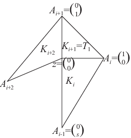
Without loss of generality we can work in the reference situation (cf. Figure 4)
Refer to caption
Figure 4: Illustration of Case a) in the proof of Theorem 1.1(b) for n>1n>1.

that Ki+1=T1K_{i+1}=T_{1}, i.e., Ai+1=(0,1)A_{i+1}=\left(0,1\right), z=(0,0)z=\left(0,0\right) and Ai−1=(0,s)A_{i-1}=\left(0,s\right) for some s<0s<0. From Theorem 3.1, in particular from (3.2), it follows that ℙn−1⟂​(Ki+1)∩ℙn−1⟂​(Ki)\mathbb{P}_{n-1}^{\perp}\left(K_{i+1}\right)\cap\mathbb{P}_{n-1}^{\perp}\left(K_{i}\right) is spanned by the polynomial q⁡(x,y):=Pn(1,3)​(1−2​x)q(x,y):=P_{n}^{(1,3)}\left(1-2x\right). Note that the adjacent triangle Ki+2K_{i+2} left to T1T_{1} lies in the left half plane. Hence qq is either positive on Ki+2K_{i+2} or negative, by which it cannot be orthogonal to all constant functions on Ki+2K_{i+2}. We conclude that

ℙn−1⟂​(Ki+2)∩ℙn−1⟂​(Ki+1)∩ℙn−1⟂​(Ki)={0}.\mathbb{P}_{n-1}^{\perp}\left(K_{i+2}\right)\cap\mathbb{P}_{n-1}^{\perp}\left(K_{i+1}\right)\cap\mathbb{P}_{n-1}^{\perp}\left(K_{i}\right)=\left\{0\right\}.

Case b) Ai+1=Qcritical​(Ki,Ai−1)A_{i+1}=Q_{\operatorname{critical}}\left(K_{i},A_{i-1}\right) and Ai−2∈ℒcritical​(Ki,Ai,z)A_{i-2}\in\mathcal{L}_{\operatorname{critical}}\left(K_{i},A_{i},z\right).
Then Ai∈ℒcritical​(Ki−1,Ai−2,z)A_{i}\in\mathcal{L}_{\operatorname{critical}}\left(K_{i-1},A_{i-2},z\right). So as in case a), but now with Ki=T1K_{i}=T_{1}, we conclude that

ℙn−1⟂​(Ki−1)∩ℙn−1⟂​(Ki)∩ℙn−1⟂​(Ki+1)={0}.\mathbb{P}_{n-1}^{\perp}\left(K_{i-1}\right)\cap\mathbb{P}_{n-1}^{\perp}\left(K_{i}\right)\cap\mathbb{P}_{n-1}^{\perp}\left(K_{i+1}\right)=\left\{0\right\}.

Case c) Ai+1=Qcritical​(Ki,Ai−1)A_{i+1}=Q_{\operatorname{critical}}\left(K_{i},A_{i-1}\right) and Ai−2∈ℒcritical​(Ki,Ai,Ai−1)A_{i-2}\in\mathcal{L}_{\operatorname{critical}}\left(K_{i},A_{i},A_{i-1}\right).

Refer to caption
Figure 5: Illustration of the geometric argument for case c). The points Ai−2,Ai−1,AiA_{i-2},A_{i-1},A_{i} are collinear and Ki∪Ki+1¯\overline{K_{i}\cup K_{i+1}} form a parallelogram.

Without loss of generality we can work in the reference configuration (see Figure 5) that Ki=T1K_{i}=T_{1} with Ai−1=(0,0)A_{i-1}=\left(0,0\right), Ai=(1,0)A_{i}=\left(1,0\right), z=(0,1)z=\left(0,1\right). Then Ki+1=convo⁡((1,0),(1,1),(0,1))K_{i+1}=\operatorname*{conv^{o}}\left((1,0),(1,1),(0,1)\right), Ki−1=convo⁡((0,0),(0,1),(s,0))K_{i-1}=\operatorname*{conv^{o}}\left((0,0),(0,1),(s,0)\right) for some s<0s<0, and Ki+2=convo⁡((0,1),(1,1),(t,u))K_{i+2}=\operatorname*{conv^{o}}\left((0,1),(1,1),(t,u)\right) with u>1u>1. From Theorem 3.1, in particular from (3.4), we conclude that ℙn−1⟂​(Ki)∩ℙn−1⟂​(Ki−1)\mathbb{P}_{n-1}^{\perp}\left(K_{i}\right)\cap\mathbb{P}_{n-1}^{\perp}\left(K_{i-1}\right) is spanned by the polynomial r⁡(x,y):=Pn(1,3)​(1−2​y)r(x,y):=P_{n}^{\left(1,3\right)}\left(1-2y\right). By arguing as in Case a) we conclude that rr is not changing sign in Ki+2K_{i+2} (since y≥1y\geq 1). Hence

ℙn−1⟂​(Ki−1)∩ℙn−1⟂​(Ki)∩ℙn−1⟂​(Ki+1)∩ℙn−1⟂​(Ki+2)={0}.\mathbb{P}_{n-1}^{\perp}\left(K_{i-1}\right)\cap\mathbb{P}_{n-1}^{\perp}\left(K_{i}\right)\cap\mathbb{P}_{n-1}^{\perp}\left(K_{i+1}\right)\cap\mathbb{P}_{n-1}^{\perp}\left(K_{i+2}\right)=\left\{0\right\}.

Case d) Ai+1=Qcritical​(Ki,Ai−1)A_{i+1}=Q_{\operatorname{critical}}\left(K_{i},A_{i-1}\right) and Ai−2=Qcritical​(Ki,Ai)A_{i-2}=Q_{\operatorname{critical}}\left(K_{i},A_{i}\right).
Without loss of generality we can consider the reference situation that Ki=T1K_{i}=T_{1} with z=(0,0)z=(0,0), Ai−2=(1,−1)A_{i-2}=(1,-1), Ai−1=(1,0)A_{i-1}=(1,0), Ai=(0,1)A_{i}=(0,1), Ai+1=(−1,1)A_{i+1}=(-1,1). From Theorem 3.1 we conclude that ℙn−1⟂​(Ki)∩ℙn−1⟂​(Ki−1)\mathbb{P}_{n-1}^{\perp}\left(K_{i}\right)\cap\mathbb{P}_{n-1}^{\perp}\left(K_{i-1}\right) is spanned by the polynomial qn​(x,y):=qn(1,0)​(x,y)q_{n}(x,y):=q_{n}^{(1,0)}(x,y) given by (3.5), and that ℙn−1⟂​(Ki+1)∩ℙn−1⟂​(Ki)\mathbb{P}_{n-1}^{\perp}\left(K_{i+1}\right)\cap\mathbb{P}_{n-1}^{\perp}\left(K_{i}\right) is spanned by the polynomial qn​(y,x)q_{n}(y,x). Since these two polynomials are linearly independent (compare the highest degree part of both polynomials), we have shown that

ℙn−1⟂​(Ki−1)∩ℙn−1⟂​(Ki)∩ℙn−1⟂​(Ki+1)={0}.\mathbb{P}_{n-1}^{\perp}\left(K_{i-1}\right)\cap\mathbb{P}_{n-1}^{\perp}\left(K_{i}\right)\cap\mathbb{P}_{n-1}^{\perp}\left(K_{i+1}\right)=\left\{0\right\}.

Case e) Ai+1∈ℒcritical2​(Ki,Ai−1)A_{i+1}\in\mathcal{L}_{\operatorname{critical}}^{2}\left(K_{i},A_{i-1}\right) and Ai−2∈ℒcritical​(Ki,Ai,Ai−1)A_{i-2}\in\mathcal{L}_{\operatorname{critical}}\left(K_{i},A_{i},A_{i-1}\right).
We can assume that Ki=T1K_{i}=T_{1} with z=(0,0)z=(0,0). Then Ai+1=(−1,c)A_{i+1}=(-1,c). From (3.6) we have that ℙn−1⟂​(Ki+1)∩ℙn−1⟂​(Ki)\mathbb{P}_{n-1}^{\perp}\left(K_{i+1}\right)\cap\mathbb{P}_{n-1}^{\perp}\left(K_{i}\right) is spanned by the polynomial q2(c,c−1)​(y,x)q_{2}^{(c,c-1)}(y,x) and from (3.3) that ℙn−1⟂​(Ki)∩ℙn−1⟂​(Ki−1)\mathbb{P}_{n-1}^{\perp}\left(K_{i}\right)\cap\mathbb{P}_{n-1}^{\perp}\left(K_{i-1}\right) is spanned by the polynomial Pn(1,3)​(2​(x+y)−1)P_{n}^{(1,3)}(2(x+y)-1). A computation shows that these two polynomials are linearly dependent iff c=2c=2. But then the inner angle at AiA_{i} equals π\pi, which we excluded.
Case f) Ai+1∈ℒcritical2​(Ki,Ai−1)A_{i+1}\in\mathcal{L}_{\operatorname{critical}}^{2}\left(K_{i},A_{i-1}\right) and Ai−2∈ℒcritical​(Ki,Ai,z)A_{i-2}\in\mathcal{L}_{\operatorname{critical}}\left(K_{i},A_{i},z\right).
Again assume that Ki=T1K_{i}=T_{1} with z=(0,0)z=(0,0). Then Ai−2=(0,s)A_{i-2}=(0,s) for some s<0s<0. We can argue as in case a), but now with Ki=T1K_{i}=T_{1}.
Case g) Ai+1∈ℒcritical2​(Ki,Ai−1)A_{i+1}\in\mathcal{L}_{\operatorname{critical}}^{2}\left(K_{i},A_{i-1}\right) and Ai−2∈ℒcritical2​(Ki,Ai)A_{i-2}\in\mathcal{L}_{\operatorname{critical}}^{2}\left(K_{i},A_{i}\right).
Again assume that Ki=T1K_{i}=T_{1} with z=(0,0)z=(0,0). Then Ai+1=(−1,c)A_{i+1}=(-1,c) and Ai−2=(d,−1)A_{i-2}=(d,-1) for some c,d∈ℝc,d\in\mathbb{R}. From (3.6) we have that ℙn−1⟂​(Ki+1)∩ℙn−1⟂​(Ki)\mathbb{P}_{n-1}^{\perp}\left(K_{i+1}\right)\cap\mathbb{P}_{n-1}^{\perp}\left(K_{i}\right) is spanned by the polynomial q2(c,c−1)​(y,x)q_{2}^{(c,c-1)}(y,x) and that ℙn−1⟂​(Ki)∩ℙn−1⟂​(Ki−1)\mathbb{P}_{n-1}^{\perp}\left(K_{i}\right)\cap\mathbb{P}_{n-1}^{\perp}\left(K_{i-1}\right) is spanned by the polynomial q2(d,d−1)​(x,y)q_{2}^{(d,d-1)}(x,y). A computation shows that these two polynomials are linearly dependent iff c=d=−3c=d=-3 or c=d=2c=d=2. But in the first case the triangles Ki−1K_{i-1} and Ki+1K_{i+1} intersect, and in the second case the inner angle at AiA_{i} equals π\pi.   

5 The intersection of nn-th degree orthogonal polynomial spaces for a triangle patch (case n=1n=1)

In this Section we will prove the intersection property Theorem 1.1(b) polynomial degrees n=1n=1. We need two simple lemmas.

Lemma 5.1

Let 𝒯:={Ki:1≤i≤q}\mathcal{T}:=\left\{K_{i}:1\leq i\leq q\right\} denote a triangle patch around z∈ℝ2z\in\mathbb{R}^{2}. Then there are Ki−1K_{i-1}, KiK_{i}, Ki+1K_{i+1} of which the barycenters are not collinear.

Proof. Let MiM_{i} be the barycenter of KiK_{i}. We will show that the points MiM_{i} (i=1,…,qi=1,\ldots,q) cannot be collinear. This will imply the statement of the Lemma.

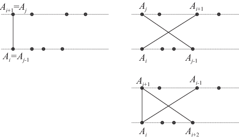
We may choose z=(0,0)z=(0,0). Suppose that the points Mi=13​(Ai−1+Ai)M_{i}=\tfrac{1}{3}(A_{i-1}+A_{i}) (i=1,…,qi=1,\ldots,q) are collinear. Then all vectors 3​(Mi−Mi−1)=Ai−Ai−23(M_{i}-M_{i-1})=A_{i}-A_{i-2} are proportional. If qq is odd then this implies that all vertices AiA_{i} are collinear, which is impossible. If qq is even then the set of vertices A1,A3,…,Aq−1A_{1},A_{3},\ldots,A_{q-1} and the set of vertices A2,A4,…,AqA_{2},A_{4},\ldots,A_{q} are both collinear and the two collinear sets lie on parallel lines. Since all vertices cannot be collinear, these two parallel lines have to be distinct. After applying an affine linear map we may assume that one of the lines is y=0y=0 with Ai=(0,0)A_{i}=(0,0) for some ii and with all other vertices on this line having coordinates (x,0)(x,0) with x>0x>0, and that the other line is y=1y=1 with Aj=(0,1)A_{j}=(0,1) for some j≠ij\neq i and with all other vertices on this line having coordinates (x,1)(x,1) with x>0x>0. First we show that j=i+1j=i+1. Indeed, if j≠i+1j\neq i+1 then the edge connecting AjA_{j} and Aj−1A_{j-1} will cross the edge connecting AiA_{i} and Ai+1A_{i+1}, which is not allowed. Thus Ai+1=(0,1)A_{i+1}=(0,1). But now the edge connecting Ai+1A_{i+1} and Ai+2A_{i+2} will cross the edge connecting AiA_{i} and Ai−1A_{i-1}, which is not allowed (see Figure 6 for this last part of the proof, where we successively arrive twice at a contradiction). Thus we cannot have two collinear sets of vertices if qq is even.   

Refer to caption
Figure 6: Illustration of the last part of the proof of Lemma 5.1 (qq even). Ai+1=AjA_{i+1}=A_{j} (left picture) because otherwise the top right picture gives a contradiction. But now the bottom picture gives a contradiction.
Lemma 5.2

Let KK be a triangle with barycenter MM. Let μ\mu be a finite measure on KK which is invariant under all affine transformations mapping KK onto itself (these form a group ismorphic with S3S_{3}). Then

∫Kp​𝑑μ=p⁡(M)​μ​(K)for all p∈ℙ1​(K).\int_{K}p\,d\mu=p(M)\,\mu(K)\quad\mbox{for all $p\in\mathbb{P}_{1}(K)$.}

This holds in particular if d​μ​(x,y)=ω⁡(x,y)​d​x​d​yd\mu(x,y)=\omega(x,y)\,dx\,dy with ω\omega the product of the barycentric coordinates for KK.

Proof. Let A,B,CA,B,C be the vertices of KK. Since the assertion is trivial for constant functions, it is sufficient to prove the property for affine linear functions pp vanishing on one of the medians A​MAM, B​MBM, C​MCM. Suppose pp vanishes on A​MAM. Then the function p−p⁡(M)p-p(M) is sent to its opposite under the affine map fixing AA and interchanging BB and CC (check this for the reference triangle TT with A=(0,0)A=(0,0), B=(1,0)B=(1,0), C=(0,1)C=(0,1)). Hence ∫K(p−p⁡(M))​𝑑μ=0\int_{K}(p-p(M))\,d\mu=0.    
Proof of Theorem 1.1(b) for n=1n=1
Let 𝒯:={Ki:1≤i≤q}\mathcal{T}:=\left\{K_{i}:1\leq i\leq q\right\} denote a triangle patch around a point z∈ℝ2z\in\mathbb{R}^{2} and let Ω:=∪i=1qKi¯\Omega:=\cup_{i=1}^{q}\overline{K_{i}}. By Lemma 5.1 there are Ki−1,Ki,Ki+1K_{i-1},K_{i},K_{i+1} such that their barycenters Mi−1,Mi,Mi+1M_{i-1},M_{i},M_{i+1} are not collinear. Now suppose that u∈ℙ1​(Ω)u\in\mathbb{P}_{1}(\Omega) and u∈ℙ0⟂​(Kj)u\in\mathbb{P}_{0}^{\perp}(K_{j}) for j=i−1,i,i+1j=i-1,i,i+1. By Lemma 5.2 we have for j∈{i−1,i,i+1}j\in\{i-1,i,i+1\} that

0=∫Kju⁡(x,y)​ωj​(x,y)​𝑑x​𝑑y∫Kjωj​(x,y)​𝑑x​𝑑y=u⁡(Mj).0=\frac{\int_{K_{j}}u(x,y)\,\omega_{j}(x,y)\,dx\,dy}{\int_{K_{j}}\omega_{j}(x,y)\,dx\,dy}=u(M_{j}).

Since the affine linear function uu vanishes on three points which are not collinear, uu is identically zero.   

Remark 5.3

If we take the triangle patch such that Ki=T1K_{i}=T_{1} with z=(0,0)z=(0,0), Ai−1=(1,0)A_{i-1}=(1,0), Ai=(0,1)A_{i}=(0,1), Ai−2=(−cd−c,1d−c)A_{i-2}=(\tfrac{-c}{d-c},\tfrac{1}{d-c}) and Ai+1=(1d′−c′,−c′d′−c′)A_{i+1}=(\tfrac{1}{d^{\prime}-c^{\prime}},\tfrac{-c^{\prime}}{d^{\prime}-c^{\prime}}), then we see from (3.7) that

ℙ0⟂​(Ki−1)∩ℙ0⟂​(Ki)∩ℙ0⟂​(Ki+1)≠{0}.\mathbb{P}_{0}^{\perp}\left(K_{i-1}\right)\cap\mathbb{P}_{0}^{\perp}\left(K_{i}\right)\cap\mathbb{P}_{0}^{\perp}\left(K_{i+1}\right)\neq\left\{0\right\}.

implies that the polynomials q1(c,d)​(x,y)q_{1}^{(c,d)}(x,y) and q1(c′,d′)​(y,x)q_{1}^{(c^{\prime},d^{\prime})}(y,x) are multiples of each other. A computation shows that then

c′=k(c−d+1),d′=k(1−d)+1(0≠k∈ℝ).c^{\prime}=k(c-d+1),\quad d^{\prime}=k(1-d)+1\qquad(0\neq k\in\mathbb{R}).

Hence Ai+1=(11−k​c,k⁡(d−c−1)1−k​c)A_{i+1}=(\tfrac{1}{1-kc},\tfrac{k(d-c-1)}{1-kc}). Then Ai+1−Ai−1A_{i+1}-A_{i-1} and Ai−Ai−2A_{i}-A_{i-2} are proportional. By the Proof of Lemma 5.1 this gives the collinearity of the barycenters of Ki−1K_{i-1}, KiK_{i} and Ki+1K_{i+1}. Thus we have shown once more that, if the barycenters of these three triangles are not collinear, then ℙ0⟂​(Ki−1)∩ℙ0⟂​(Ki)∩ℙ0⟂​(Ki+1)={0}\mathbb{P}_{0}^{\perp}\left(K_{i-1}\right)\cap\mathbb{P}_{0}^{\perp}\left(K_{i}\right)\cap\mathbb{P}_{0}^{\perp}\left(K_{i+1}\right)=\left\{0\right\}.

6 Injectivity for the polynomial projection
operator: some follow-up

Recall Theorem 1.1(c) about the injectivity of the polynomial projection operator Πn𝒯:ℙn​(Ω)→ℙn−1​(𝒯)\Pi_{n}^{\mathcal{T}}\colon\mathbb{P}_{n}(\Omega)\to\mathbb{P}_{n-1}(\mathcal{T}), Let ‖⋅‖𝒯:=(⋅,⋅)𝒯1/2\left\|\cdot\right\|_{\mathcal{T}}:=\left(\cdot,\cdot\right)_{\mathcal{T}}^{1/2} and define

cn′​(𝒯)\displaystyle c_{n}^{\prime}(\mathcal{T}) :=infv∈ℙn​(Ω)\{0}(v,Πn𝒯​v)𝒯(v,v)𝒯=infv∈ℙn​(Ω)\{0}‖Πn𝒯​v‖𝒯2‖v‖𝒯2>0,\displaystyle:=\inf_{v\in\mathbb{P}_{n}(\Omega)\backslash\{0\}}\frac{(v,\Pi_{n}^{\mathcal{T}}v)_{\mathcal{T}}}{(v,v)_{\mathcal{T}}}=\inf_{v\in\mathbb{P}_{n}(\Omega)\backslash\{0\}}\frac{\|\Pi_{n}^{\mathcal{T}}v\|_{\mathcal{T}}^{2}}{\|v\|_{\mathcal{T}}^{2}}>0, (6.1)
cn′′​(𝒯)\displaystyle c_{n}^{\prime\prime}(\mathcal{T}) :=infv∈ℙn​(Ω)\{0}‖v‖𝒯2‖v‖L2​(Ω)2>0,\displaystyle:=\inf_{v\in\mathbb{P}_{n}(\Omega)\backslash\{0\}}\frac{\|v\|_{\mathcal{T}}^{2}}{\|v\|_{L^{2}(\Omega)}^{2}}>0, (6.2)
cˇn​(𝒯)\displaystyle\check{c}_{n}(\mathcal{T}) :=infv∈ℙn​(Ω)\{0}(v,Πn𝒯​v)𝒯(v,v)L2​(Ω)≥cn′′​(𝒯)​cn′​(𝒯)>0.\displaystyle:=\inf_{v\in\mathbb{P}_{n}(\Omega)\backslash\{0\}}\frac{(v,\Pi_{n}^{\mathcal{T}}v)_{\mathcal{T}}}{(v,v)_{L^{2}(\Omega)}}\geq c_{n}^{\prime\prime}(\mathcal{T})c_{n}^{\prime}(\mathcal{T})>0. (6.3)

The inequality in (6.1) follows from the injectivity of Πn𝒯\Pi_{n}^{\mathcal{T}}, while the inequality in (6.2) is a consequence of the equivalence of all norms on a finite dimensional space.

Remark 6.1

We can expand the squared norms in (6.1) and (6.2). Let Λi\Lambda_{i} be the orientation preserving affine linear map of T1T_{1} onto KiK_{i} which sends (0,0)(0,0) to zz. Let {pm}m=1,…,n⁡(n+1)/2\{p_{m}\}_{m=1,\ldots,n(n+1)/2} be an orthonormal basis for ℙn−1​(T1)\mathbb{P}_{n-1}(T_{1}) with respect to the weight function ω\omega on T1T_{1}. Then

∥Πn𝒯v∥𝒯2=∑i=1qdetΛi∑m=112​n​(n+1)\displaystyle\big\|\Pi_{n}^{\mathcal{T}}v\big\|_{\mathcal{T}}^{2}=\sum_{i=1}^{q}\det\Lambda_{i}\sum_{m=1}^{\frac{1}{2}n(n+1)} (∫T1v∘Λi​pm​ω)2,\displaystyle\left(\int_{T_{1}}v\circ\Lambda_{i}\;p_{m}\,\omega\right)^{2},
‖v‖𝒯2=∑i=1qdetΛi​∫T1(v∘Λi)2​ω,\displaystyle\|v\|_{\mathcal{T}}^{2}=\sum_{i=1}^{q}\det\Lambda_{i}\int_{T_{1}}(v\circ\Lambda_{i})^{2}\,\omega,\qquad ‖v‖L2​(Ω)2=∑i=1qdetΛi​∫T1(v∘Λi)2.\displaystyle\|v\|_{L^{2}(\Omega)}^{2}=\sum_{i=1}^{q}\det\Lambda_{i}\int_{T_{1}}(v\circ\Lambda_{i})^{2}.

Hence cn′′=cn′′​(𝒯)c_{n}^{\prime\prime}=c_{n}^{\prime\prime}(\mathcal{T}) is independent of the choice of the patch 𝒯\mathcal{T} and it equals

cn′′=infv∈ℙn​(T1)\{0}∫T1v​(x,y)2​x​y​(1−x−y)​𝑑x​𝑑y∫T1v​(x,y)2​𝑑x​𝑑y.c_{n}^{\prime\prime}=\inf_{v\in\mathbb{P}_{n}(T_{1})\backslash\{0\}}\frac{\int_{T_{1}}v(x,y)^{2}\,x\,y\,(1-x-y)\,dx\,dy}{\int_{T_{1}}v(x,y)^{2}\,dx\,dy}\,. (6.4)
Remark 6.2

From [21, Prop. 3.46] there follows an nn-explicit lower bound for cn′′c_{n}^{\prime\prime} as given by (6.4): cn′′≥C/(n+1)4c_{n}^{\prime\prime}\geq C/(n+1)^{4} with a fixed nn-independent constant C>0C>0.

Since the quotients of integrals in (6.1)–(6.3) are invariant under affine linear maps, we might restrict to the case that K1K_{1} is the reference triangle T1T_{1}. But in view of the numerical applications, we consider only translations and rotations of triangle patches. Thus we restrict in the following to the case that z=0z=0 and Aq=(rq,0)A_{q}=(r_{q},0) for some rq>0r_{q}>0. The further data determining 𝒯\mathcal{T} are, for i=1,…,qi=1,\ldots,q, the angles αi,βi,γi\alpha_{i},\beta_{i},\gamma_{i} of the triangle KiK_{i} at z,Ai−1,Aiz,A_{i-1},A_{i}, respectively, together with the length rir_{i} of the edge connecting zz with AiA_{i} (see Figure 7).

Refer to caption
Figure 7: Illustration of angles α1,βi,γi\alpha_{1},\beta_{i},\gamma_{i}, and radii rir_{i} for a triangle patch.

Evident constraints on these numbers are that αi+βi+γi=π\alpha_{i}+\beta_{i}+\gamma_{i}=\pi and α1+⋯+αq=2​π\alpha_{1}+\cdots+\alpha_{q}=2\pi. But 𝒯\mathcal{T} would already be completely determined by α2,…,αq\alpha_{2},\ldots,\alpha_{q}, β2,…,βq\beta_{2},\ldots,\beta_{q} and rqr_{q}, or by α2,…,αq\alpha_{2},\ldots,\alpha_{q} and r1,…,rqr_{1},\ldots,r_{q}. The map (α2,…,αq,β2,…,βq,rq)↔(α2,…,αq,r1,…,rq)(\alpha_{2},\ldots,\alpha_{q},\beta_{2},\ldots,\beta_{q},r_{q})\leftrightarrow(\alpha_{2},\ldots,\alpha_{q},r_{1},\ldots,r_{q}) is continuous in both directions, as can be seen from the following identities obtained by a combination of the sine rule and the cosine rule for the triangle KiK_{i} :

sin⁡αiri−12+ri2−2ri−1ricosαi=sin⁡βiri=sin⁡(π−αi−βi)ri−1.\frac{\sin\alpha_{i}}{\sqrt{r_{i-1}^{2}+r_{i}^{2}-2r_{i-1}r_{i}\cos\alpha_{i}}}=\frac{\sin\beta_{i}}{r_{i}}=\frac{\sin(\pi-\alpha_{i}-\beta_{i})}{r_{i-1}}\,. (6.5)

The quotients of integrals in (6.1)–(6.3) will depend continuously on vv and the data of 𝒯\mathcal{T}. Therefore, the three constants in (6.1)–(6.3) will depend continuously on the data of 𝒯\mathcal{T} and they will remain bounded away from zero if we let range the data of 𝒯\mathcal{T} over a compact set. To fix a compact set, choose δ∈(0,π/3]\delta\in(0,\pi/3] and ρ>0\rho>0.

Definition 6.3

The compact set of triangle patches Xq,δ,ρX_{q,\delta,\rho} consists of all 𝒯\mathcal{T} with αi,βi,γi≥δ\alpha_{i},\beta_{i},\gamma_{i}\geq\delta and ri≥ρr_{i}\geq\rho (i=1,…,qi=1,\ldots,q). Furthermore define

c~n​(q,δ,ρ):=inf𝒯∈Xq,δ,ρcˇn​(𝒯).\tilde{c}_{n}(q,\delta,\rho):=\inf_{\mathcal{T}\in X_{q,\delta,\rho}}\check{c}_{n}(\mathcal{T}). (6.6)

By the second equality in (6.5) we see that, for given δ\delta and qq there exists C>0C>0 such that ρ≤ri≤C​ρ\rho\leq r_{i}\leq C\rho (OPENi=1,…,q)i=1,\ldots,q) if 𝒯∈Xq,δ,ρ\mathcal{T}\in X_{q,\delta,\rho}. Since the quotients of integrals in (6.1)–(6.3) are invariant under dilations, c~n​(q,δ,ρ)\tilde{c}_{n}(q,\delta,\rho) will be independent of ρ\rho. Since necessarily q​δ≤2​πq\delta\leq 2\pi, Xq,δ,ρX_{q,\delta,\rho} is non-empty for only finitely many values of qq. We conclude:

Theorem 6.4

infρ>0,q≥3c~n​(q,δ,ρ)>0\displaystyle\inf_{\rho>0,\;q\geq 3}\tilde{c}_{n}(q,\delta,\rho)>0.

References

  • [1] M. Ainsworth and J. T. Oden. A posteriori error estimation in finite element analysis. Wiley, 2000.
  • [2] I. Babuška and W. C. Rheinboldt. A-posteriori error estimates for the finite element method. Internat. J. Numer. Meth. Engrg., 12:1597–1615, 1978.
  • [3] I. Babuška and W. C. Rheinboldt. Error estimates for adaptive finite element computations. SIAM J. Numer. Anal., 15:736–754, 1978.
  • [4] W. Bangerth and R. Rannacher. Adaptive finite eement methods for differential equations. Birkhäuser, Basel, 2003.
  • [5] R. E. Bank and A. Weiser. Some a posteriori error estimators for elliptic partial differential equations. Math. Comp., 44:283–301, 1985.
  • [6] R. E. Bank and J. Xu. Asymptotically exact a posteriori error estimators. II. General unstructured grids. SIAM J. Numer. Anal., 41:2313–2332, 2003.
  • [7] P. Binev, W. Dahmen, and R. DeVore. Adaptive finite element methods with convergence rates. Numer. Math., 97:219–268, 2004.
  • [8] F. A. Bornemann, B. Erdmann, and R. Kornhuber. A posteriori error estimates for elliptic problems in two and three space dimensions. SIAM J. Numer. Anal., 33:1188–1204, 1996.
  • [9] W. Dörfler. A convergent adaptive algorithm for Poisson’s equation. SIAM J. Numer. Anal., 33:1106–1124, 1996.
  • [10] W. Dörfler and R. H. Nochetto. Small data oscillation implies the saturation assumption. Numer. Math., 91:1–12, 2002.
  • [11] M. Dubiner. Spectral methods on triangles and other domains. J. Sci. Comput., 6:345–390, 1991.
  • [12] C. F. Dunkl and Y. Xu. Orthogonal polynomials of several variables. Encyclopedia of Mathematics and its Applications, Vol. 81. Cambridge University Press, Cambridge, 2001.
  • [13] J. S. Hesthaven and T. Warburton. Nodal high-order methods on unstructured grids. I. Time-domain solution of Maxwell’s equations. J. Comput. Phys., 181:186–221, 2002.
  • [14] G. E. Karniadakis and S. J. Sherwin. Spectral/h​php element methods for computational fluid dynamics. Numerical Mathematics and Scientific Computation. Oxford University Press, Oxford, second edition, 2005.
  • [15] T. Koornwinder. Two-variable analogues of the classical orthogonal polynomials. In Theory and application of special functions, pages 435–495. Academic Press, New York, 1975.
  • [16] K. Mekchay and R. H. Nochetto. Convergence of adaptive finite element methods for general second order linear elliptic PDEs. SIAM J. Numer. Anal., 43:1803–1827, 2005.
  • [17] J. Proriol. Sur une famille de polynomes à deux variables orthogonaux dans un triangle. C. R. Acad. Sci. Paris, 245:2459–2461, 1957.
  • [18] S. Repin. A posteriori estimates for partial differential equations, volume 4. Walter de Gruyter, Berlin, 2008.
  • [19] R. Stevenson. Optimality of a standard adaptive finite element method. Found. Comput. Math., 7:245–269, 2007.
  • [20] G. Szegő. Orthogonal polynomials. Colloquium Publications, Vol. XXIII. American Mathematical Society, Providence, R.I., fourth edition, 1975.
  • [21] R. Verfürth. A posteriori error estimation techniques for finite element methods. Numerical Mathematics and Scientific Computation. Oxford University Press, Oxford, 2013.