Technical Report: An MGF-based Unified Framework to Determine the Joint Statistics of Partial Sums of Ordered i.n.d. Random Variables
Abstract
The joint statistics of partial sums of ordered random variables (RVs) are often needed for the accurate performance characterization of a wide variety of wireless communication systems. A unified analytical framework to determine the joint statistics of partial sums of ordered independent and identically distributed (i.i.d.) random variables was recently presented. However, the identical distribution assumption may not be valid in several real-world applications. With this motivation in mind, we consider in this paper the more general case in which the random variables are independent but not necessarily identically distributed (i.n.d.). More specifically, we extend the previous analysis and introduce a new more general unified analytical framework to determine the joint statistics of partial sums of ordered i.n.d. RVs. Our mathematical formalism is illustrated with an application on the exact performance analysis of the capture probability of generalized selection combining (GSC)-based RAKE receivers operating over frequency-selective fading channels with a non-uniform power delay profile. We also discussed a couple of other sample applications of the generic results presented in this work.
Index Terms:
Order statistics, Joint statistics, Non-identical distribution, Moment generating function (MGF), Probability density function (PDF), Exponential distribution.I Introduction
The subject of order statistics deals with the properties and distributions of the ordered random variables (RVs) and their functions. It has found applications in many areas of statistical theory and practice [1], with examples in life-testing, quality control, radar, as well as signal and image processing [2, 3, 4, 5, 6, 7, 8]. Order statistics has made over the last decade an increasing number of appearances in the design and analysis of wireless communication systems, specifically for the performance analysis of advanced diversity techniques, adaptive transmission techniques, and multiuser scheduling techniques (see for example [9, 10, 11, 12, 13, 14, 15, 16, 17, 18, 19, 20, 21, 22]). In these performance analysis exercises, the joint statistics of partial sums of ordered RVs are often necessary for the accurate characterization of system performance [12, 19, 23]. Note that even if the original unordered RVs are independently distributed, their ordered versions are dependent due to the inequality relations among them, which makes it challenging to such joint statistics. Recently, a successive conditioning approach was used to convert dependent ordered random variables into independent unordered ones [10, 11]. However, this approach requires some case-specific manipulations, which may not always be generalizable.
Motivated by these facts, we introduced in [24] a unified analytical framework to determine the joint statistics of partial sums of ordered independent and identically distributed (i.i.d.) RVs by extending the interesting results published in [25, 26, 4]. More specifically, our approach can be applied not only to the cases when all the ordered RVs are involved but also to the cases when only the best RVs are considered. With the proposed approach, we can systematically derive the joint statistics of any partial sums of ordered statistics, in terms of the moment generating function (MGF) and the probability density function (PDF). These statistical results can be used for the performance analysis of various wireless communication systems over generalized fading channels [9]. However, the identical fading assumption on all diversity branches is not always valid in real-life applications. The average fading power may vary from one path to the other because the branches of a diversity system are sometimes unbalanced and the communication system is sometimes operating over frequency-selective channels with a non-uniform power delay profile or channel multipath intensity profile (i.e. the average SNR of the diversity paths are not necessary the same).
We therefore introduce in this paper an unified analytical framework to determine the joint statistics of partial sums of ordered independent non-identically distributed (i.n.d.) RVs by extending our previous work for i.i.d. fading scenarios [24]. More specifically, we use an MGF based systematic analytical approach to investigate the joint statistics of any partial sums of ordered statistics for general i.n.d. fading, in terms of MGF and the PDF. We would like to emphasize that such generalization.The main challenge for generalizing the work in [24] to i.n.d. general fading cases is that joint PDF of ordered i.n.d. RVs is much more complicated than that of ordered i.i.d. RVs. We need to carry out more detailed manipulation and introduce new mathematical representation to obtain the generic results (e.g. joint MGF and related joint PDF) for i.n.d. general cases in a compact form. In addition, we present the closed-form expressions for the exponential RV special case, which is most widely used in wireless literature. For other type of RVs, our approach will lead to much simpler results than the conventional approach involving multiple-fold integration. Furthermore, the exponential distribution is frequently used in the performance evaluation analysis of networks and telecommunication systems. It is also used to model the waiting times between occurrences of rare events, lifetimes of electrical or mechanical devices [27, 3, 2, 28]. Finally, as an application of our analytical framework, we generalize the performance results of GSC-based RAKE receivers in [23] by maintaining the assumption of independence among the diversity paths but relaxing the identically distributed assumption. We also discussed a couple of other sample applications of the generic results presented in this work.
II Problem Statement and Main Idea
Order statistics deals with the distributions and statistical properties of the new random variables obtained after ordering the realizations of some random variables. Let , denote i.n.d. nonnegative random variables with PDF and CDF . Let denote the random variable corresponding to the -th largest observation of the original random variables (also called -th order statistics), such that . The -dimensional joint PDF of the ordered RVs is given by [1]
| (1) |
Similarly, the -dimensional joint PDF of is given by [1]
| (2) | |||||
The objective is to derive the joint PDF of partial sums involving either all or the first () ordered RVs for the more general case in which the diversity paths are independent but not necessarily identically distributed. Similar to [24], we adopt a general two-step approach:
-
Step I: Obtain the analytical expressions of the joint MGF of partial sums (not necessarily the partial sums of interest as will be seen later).
-
Step II: Apply inverse Laplace transform to derive the joint PDF of partial sums (additional integration may be required to obtain the desired joint PDF).
In step I, by interchanging the order of integration, while ensuring each pair of limits is chosen to be as tight as possible, the multiple integral can be rewritten into compact equivalent representations. After obtaining the joint MGF in a compact form, we can derive joint PDF of selected partial sum through inverse Laplace transform. For most cases of our interest, the joint MGF involves basic functions, for which the inverse Laplace transform can be calculated analytically. In the worst case, we may rely on the Bromwich contour integral. In most of the case, the result involves a single one-dimensional contour integration, which can be easily and accurately evaluated numerically with the help of integral tables [29, 30] or using standard mathematical packages such as Mathematica and Matlab.
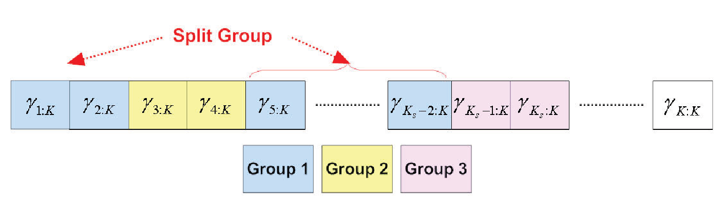
The above general steps can be directly applied when all ordered RVs are considered and the RVs in the partial sums are continuous. When either of these conditions do not hold, we need to apply some extra steps in the analysis in order to obtain a valid joint MGF [24]. For example, when the RVs involved in one partial sum is not continuous, i.e., separated by the other RVs, we need to divide these RVs into smaller sums. For example in Fig. 1, we consider 3-dimensional joint PDF of , , , , , and for . Note that the first group is not continuous. As a result, we will derive 5-dimensional joint MGF in step I, , , , , . After the joint PDF of the new substituted partial sums are derived with inverse Laplace transform in step II, we can transform it to a lower dimensional desired joint PDF with finite integration.
III Common Functions and Useful Relations
In the following sections, we present several examples to illustrate the proposed analytical framework. Our focus is on how to obtain compact expressions of the joint MGFs for i.n.d. general fading conditions, which can be greatly simplified with the application of the following function and relations.
III-A Common Functions
- i)
A mixture of a CDF and an MGF :
(3) where denotes the PDF of the RV of interest. Note that is the CDF and leads to the MGF. Here, the variable is real, while can be complex.
- ii)
A mixture of an exceedance distribution function (EDF) and an MGF, :
(4) Note that is the EDF while gives the MGF.
- iii)
An interval MGF :
(5) Note that gives the MGF.
Note that the functions defined in (3), (4) and (5) are related as follows:
| (6) | |||||
| (7) |
III-B Simplifying Relationship
- i)
Integral :
Based on the derivation given in Appendix A, the integral defined as:(8) can be simply expressed in terms of the function as
(9) In here, the complicated summation notation used in eq. (8) is simplified based on the following power set definition. We define index set as . The subset of with elements is denoted by . The remaining index can be grouped in the set . Based on these definitions, a summation in (8) includes all possible subsets of the index set excluding the subset with elements and these subsets with elements can be denoted by .
- ii)
Integral :
Following the similar derivation as given in Appendix B, the integral , defined as(10) can be simply re-written in terms of the function with the help of the definition of power set used in III-B-i) as
(11) - iii)
Integral :
Based on the derivation given in Appendix C, the integral , defined as(12) can be simply re-written in terms of the function as
(13)
IV Sample Cases when All Ordered RVs are Considered
Theorem IV.1
(PDF of among ordered RVs)
Let for convenience. We can derive the PDF of as
| (14) | |||||
where denotes the inverse Laplace transform with respect to .
Proof:
The MGF of is given by the expectation
| (15) | |||||
where denotes the expectation operator. By applying (9), we can obtain the MGF of as
| (16) |
Therefore, we can derive the PDF of by applying the inverse Laplace transform as
| (17) | |||||
∎
Theorem IV.2
(Joint PDF of and )
Let and for convenience, then we can derive the 2-dimensional joint PDF of as
| (18) | |||||
Proof:
The second order MGF of is given by the expectation
| (19) | |||||
We show in Appendix D that by applying (9) and [24, Eq. (2)] and then (11), we can obtain the second order MGF of as
| (20) | |||||
Again, letting and , we can obtain the desired 2-dimensional joint PDF of and by applying the inverse Laplace transform as
| (21) | |||||
∎
Theorem IV.3
(Joint PDF of and )
Let and for convenience. We can obtain the 2-dimensional joint PDF of as
| (22) |
V Sample cases when only ordered RVs are considered
Let us now consider the cases where only the best () ordered RVs are involved.
Theorem V.1
(PDF of , )
Let for convenience, then we can derive the PDF of as
| (23) |
where
| (24) | |||||
Proof:
We only need to consider separately in this case. Let and . The target second order MGF of is given by the expectation in
| (25) | |||||
By simply applying [24, Eq. (2)] and then (11) to (25), we can obtain the second order MGF result as
| (26) | |||||
Again, letting and , we can obtain the 2-dimensional joint PDF of and by applying the inverse Laplace transform as
| (27) | |||||
Finally, noting that , we can obtain the target PDF of with the following finite integration
| (28) |
∎
Theorem V.2
(Joint PDF of and for )
Let and , then the joint PDF of can be obtained as
| (29) | |||||
Proof:
For the joint PDF of and , as one of original groups is split by , we should consider substituted groups for the split group instead of original groups as shown in Fig. 2. As a result, we will start by obtaining a four order MGF. In this case, the higher dimensional joint PDF can then be used to find the desired 2-dimensional joint PDF of interest by transformation.
Applying the results in [24, Eq. (2)], (9), (11) and (13), we derive in Appendix E the target joint MGF. Let , , , and , then
| (30) | |||||
Starting from the MGF expressions given above, we apply inverse Laplace transforms in Appendix E in order to derive the following joint PDFs
| (31) | |||||
∎Note that (29) involves only finite integrations of joint PDFs. Therefore, while a generic closed-form expression is not possible, the desired joint PDF can be easily numerically evaluated with the help of integral tables [29, 30] or using standard mathematical packages, such as Mathematica or Matlab etc.
Theorem V.3
(Joint PDF of and )
Let and , then we can simply obtain the joint PDF of as
| (32) | |||||
Proof:
Omitted. ∎Note again that only the finite integrations of joint PDFs are involved.
VI Closed-form expressions for exponential RV case
Now, we focus on obtaining the joint PDFs for i.n.d. exponential RV special cases in a ready-to-use form. The PDF and the CDF of the RVs are given by and for , respectively, where is the average of the -th RV.
The above novel generic results are quite general and apply to any RVs. We now focus on obtaining the joint PDFs for i.n.d. exponential RV special cases in a ready-to-use form and illustrate in this section some results for the independent non-identical exponential RV special case, where the PDF and the CDF of are given by and for , respectively, where is the average of the -th RV. As shown in Appendix F, (9), (11) and (13) can be specialized to
- i)
For special case:
(33) (34) (35) - ii)
For general case:
(36) (37) (38) where
(39) (40)
After substituting (36), (37) and (38) into the derived expressions of the joint PDF of partial sums of ordered statistics presented in the previous sections, it is easy to derive the following closed-form expressions for the PDFs by applying the classical inverse Laplace transform pair and the property given in [24, Appendix I]. While some of these results have been derived using the successive conditioning approach previously, we list them here for the sake of convenience and completeness in the next page.
- 1)
PDF of :
(41) where
(42) - 2)
Joint PDF of and :
(43) where
(44) (45) (46) - 3)
Joint PDF of and :
(47) where
(48) (49) (50) - 4)
PDF of :
(51) where
(52) (53) - 5)
Joint PDF of and for :
(54) where
(55) (56) (57) (58) (59) (60)
VII Application Example
The above derived joint PDFs of partial sums of ordered statistics can be applied to the performance analysis of various wireless communication systems. In this section, we discuss several selected application examples.
VII-A Derivation of the Capture Probability of GSC RAKE receiver over i.n.d. Rayleigh fading conditions
Recently, we presented the exact performance analyses of the capture probability on GSC RAKE receivers in [23]. For analytical simplification, the fading was assumed both independent and identically distributed from path to path. However, the average SNR of each path (or branch) is different for most practical channel models, especially for wide-band SS signals since the average fading power may vary from one path to the other. For example, experimental measurements indicate that the radio channel is characterized by an exponentially decaying multipath intensity profile (MIP) for indoor office buildings [31] as well as urban [32] and suburban areas [33]. Based on this motivation in mind, with the help of our derived results in Sec V, we can extend our previous result (a closed-form formula of the capture probability on GSC RAKE receivers) by maintaining the assumption of independence among the diversity paths but relaxing the identically distributed assumption.
Let be the order statistics obtained by arranging nonnegative i.n.d. RVs, , in decreasing order of magnitude such that . Based on the system model and definition in [23], the capture probability can be written as
| (61) |
where and . If we assume , and , then (61) can be calculated in terms of the 2-dimensional joint PDF of and easily as
| (62) |
The joint PDF of and , can be derived with the help of our extended approach in this paper. More specifically, inserting (47) into (62), the closed-form expression for i.n.d. Rayleigh fading conditions is shown at the top of the next page (refer to Appendix-G for details).
| (63) | |||||
The closed-form expressions of integral parts in the expression presented in (63) can be derived as
- i)
The first integral part:
(64) - ii)
The second integral part:
(65) - iii)
The third integral part:
(66) - iv)
The forth integral part:
(67) - v)
The fifth integral part:
(68) - vi)
The sixth integral part:
(69)
VII-B Finger Replacement Schemes for RAKE Receivers in the Soft Handover Region over i.n.d. fading channels
Recently, new finger replacement techniques for RAKE reception in the soft handover (SHO) region [34] has been proposed and analyzed over independent and identical fading (i.i.d.) channel. The proposed schemes are basically based on the block comparison among groups of resolvable paths from different base stations and lead to the reduction of complexity while offering commensurate performance. If we let , and (for ), where () and () are the order statistics obtained by arranging nonnegative i.n.d. path SNRs corresponding to the th base station () in descending order, then the RAKE combiner output SNR with GSC is given by . and are dependent but and are independent. In practice, the i.i.d. fading assumption on the diversity paths is not always realistic due to, for example, the different adjacent multipath routes with the same path loss. Although non-identical fading is important for practical implementation, [34] have only investigated the non-uniform power delay profile case only through computer simulation due to the high analysis complexity. The major difficulty in this problem is to derive the joint statistics of ordered exponential variates over non-identical fading assumptions, which can be obtained by applying Theorem V.1 and V.3 of section V. Due to space limitation, the analytical details are omitted in this work.
VII-C Outage Probability of GSC RAKE Receivers Over i.n.d. Rayleigh Fading Channel subject to self-interference
Recently, the outage probability of GSC RAKE receivers subject to self-interference over independent and identically distributed Rayleigh fading channels has been investigated in [23]. Let be the SNR of the -th diversity path and () be the order statistics obtained by arranging nonnegative i.n.d. RVs, , in decreasing order of magnitude such that . Then, the outage probability, denoted by , is then defined as [23],
| (70) |
where is the outage threshold and is the self-interference cancellation coefficient (in practice, each path may have the different value of ). The closed-form expression for this outage probability over i.i.d. Rayleigh fading paths has been derived and compared to that of partial RAKE receivers. However, the average signal-to-noise ratio (SNR) of each path (or branch) is different for most practical channel models, especially for wide-band spread spectrum signals. As results, to evaluate the outage probability over i.n.d. fading channel subject to self-interference, the major difficulty is to derive the joint PDF of and for i.n.d. case. Fortunately, the target joint PDF can be obtained with the help of Theorem IV.2 in Section IV.
Appendices
Appendix A Derivation of
In this appendix, we derive Eq. (9). At first, we derive special case and then we extend this result to general case for arbitrary and .
A-A Special Case
| (72) |
To simply (72), we consider separately.
- i)
for
In this case, we can obtain the following result by deploying (72) as(73) In (73), noting that , after applying integration by part similar to [24], we can obtain the following result
(74) (75) (76) - ii)
- iii)
From results (75), (78), and (80), we can finally simplify (71) as
| (81) |
A-B General Case
With arbitrary and , we can re-write (71) as
| (82) | |||||
Appendix B Derivation of
In this appendix, we derive Eq. (11). At first, we similarly derive special case and and then we extend this result to general case for arbitrary and .
B-A Special Case
B-B General Case
With arbitrary and , we can re-write (84) as
| (86) | |||||
Appendix C Derivation of
In this appendix, we show the derivation of Eq.(13). Similar to the derivation progress of (9) and (11), we first derive special case and and then we extend this result to general case for arbitrary and .
C-A Special Case
Let us first consider and case as
| (88) |
In here, by deploying (88), (88) can be re-written as
| (89) |
In (89), using similar manipulations with (74) to the ones used in the previous Appendices A and B, the first, the second and the third multiple integral terms can be also re-written as, respectively
| (90) |
| (91) |
| (92) |
Similarly in (89), the -th, -th and the final multiple integral terms can be also re-written as respectively
| (93) |
| (94) |
| (95) |
Using all the above results from (90) to (95) in (89) and then after some manipulations similar to the one used in previous Appendices A and B, (89) can be simplified as
| (96) |
In (96), after applying (74) to the first integral terms and then some manipulations, it can be simply re-written as
| (97) |
Using (97) in (96), (96) can be simplified as
| (98) |
In (98), after applying (74) to the first integral terms with the help of similar manipulations used in (97), the first integral terms in (98) can be simply re-written as
| (99) |
Now, using (99), after adding (99) and the second integral term in (98), we can obtain the following result
By simplifying (101), we can obtain the final closed-form for special case and as
| (102) | |||
| (103) |
C-B General Case
With arbitrary and , we can also re-write (88) as
| (104) | |||||
Appendix D Derivation of (20)
Starting with (19), with the help of integral solution, (19) can be simply re-written as
| (106) |
In (106), by simply applying (9) and (11), we can easily obtain each of the following results
| (107) | |||
| (108) |
By inserting (107) and (108) in order into (19), we can obtain the second order MGF of and as
| (109) | |||||
Appendix E Derivation of the joint PDF of and for among ordered RVs
In this Appendix, we derive the joint PDF of and among ordered RVs by considering .
Let , , and . The 4-dimensional MGF of is given by the expectation
| (110) |
With the help of integral solution presented in [24], (9), (11) and (13), we can easily obtain the 4-dimensional MGF of , , and as
| (111) |
Having a MGF expression given in (111), we are now in the position to derive the 4-dimensional joint PDF of , , and . Letting , , , and we can derive the 4-dimensional PDF of , , and by applying an inverse Laplace transform yielding
| (112) |
With this 4-dimensional joint PDF, letting and we can obtain the 2-dimensional joint PDF of by integrating over and yielding
| (113) |
or equivalently we can obtain the 2-dimensional joint PDF of by integrating over and giving
| (114) |
Appendix F Derivation of Multiple Product of Common Functions
In VI-ii), (36), (37), and (38) have the form of multiple product of (33), (34), and (35), respectively. Therefore, to apply an inverse LT for deriving final PDF closed-form expressions from MGF expressions, a multiple product expression needs to be converted to a summation expression of function. In this appendix, we derive simple summation expressions of function from multiple product expressions. To derive them, the following four formulas should be converted to a summation expression.
- i)
At first, we derive special case for a) the multiple product from to and then we extend this result to general case for b) the multiple product from arbitrary to .
For case a), we need to convert the following multiple product from to to a summation expression.
(115) With (115), after deploying the multiple product term and then rearrange and simplify them, the multiple product term can be converted to the summation expression of just as
(116) where ,
(117) (118) For the case of the multiple product from arbitrary to , after applying the same derivation progress as (116), we can obtain the final result as
(119) where
(120) (121) - ii)
Similar to F-i), at first, we derive special case for a) the multiple product from to and then we extend this result to general case for b) the multiple product from arbitrary to .
For case a), after deploying the multiple product term of exponential function from to and then simplify them, the multiple product term can be converted to the summation expression of as
(122) where .
For case b), after applying the same derivation progress as (122), the multiple product from arbitrary to can be obtained as
(123) - iii)
Similar to F-i) and ii), especially, using the similar manipulation used in F-i) and ii) in (123), the final simple summation expression from arbitrary to can be obtained as
(124) - iv)
In this case, with the help of the property of exponential multiplication, we can easily derive the summation expression from the multiple product expression from arbitrary to , respectively, as
(125)
Based on the above results, we can now obtain the summation expressions of (33), (34), and (35) for arbitrary to . With (33), (34), and (35), we can write the multiple product of (33), (34), and (35) for arbitrary to respectively as
| (126) |
| (127) |
| (128) |
For the summation expression of the multiple product of (33) for arbitrary to , using (119) and (123) in (126), we can obtain the final summation closed-form expression (36).
Appendix G Capture Probability of GSC RAKE receivers
G-A Joint PDF
In (129), there are two integral expressions and the first integral part can be directly derived as the following closed form expression
| (130) |
However, for the second integral part, we need to consider two cases separately based on the valid integral region of , , and as
| (131) |
With simplified (131), we can get the following closed-form expressions, respectively, as
| (132) |
and
| (133) |
G-B Capture Probability
Starting from (62), inserting the closed-form expression of (47) presented in G-A into (62), the closed-form expression for i.n.d. Rayleigh fading conditions can be written in (63). In (63), there are six double-integral expressions. For the first and second cases, we can directly obtain the closed-from expression as shown in (64) and (65). However, for others, we need to carefully consider the valid integral region respectively as
- iii)
The third integral expression:
In this case, for valid integration, we need to consider two cases separately. If , then and . If , then and . As a result, we can re-write the third integral expression as(134) From (134), we can directly derive the closed-form expressions as
(135) and
(136) - iv)
The forth integral expression:
In this case, similar to the case iii), we also need to consider two cases separately. As a result, we can re-write the forth integral expression as(137) With (137), we can also directly derive the closed-form expressions as
(138) and
(139) - v)
The fifth integral expression:
In this case, we need to consider two cases separately for valid integration. If , then and . If , then there is no valid overlap integration region. As a result, we can re-write the third integral expression as(140) With (140), we can also directly derive the closed-form expressions as
(141) - vi)
The sixth integral expression:
In this case, similar to the case v), we also need to consider two cases separately. As a result, we can re-write the forth integral expression as
References
- [1] H. A. David, Order Statistics. New York, NY: John Wiley & Sons, 1981.
- [2] N. Balakrishnan and C. R. Rao, Handbook of Statistics 17: Order Statistics: Applications, 2nd ed. North-Holland: Elsevier, 1998.
- [3] A. Goldsmith, Wireless Communications. New York, NY: Cambridge University Press, 2005.
- [4] A. H. Nuttall and P. M. Baggenstoss, “Joint distributions for two useful classes of statistics, with applications to classification and hypothesis testing,” IEEE Trans. Signal Processing, submitted for publication. [Online]. Available: http://www.npt.nuwc.navy.mil/Csf/papers/order.pdf
- [5] S. M. Kay, A. H. Nuttall, and P. M. Baggenstoss, “Multidimensional probability density function approximations for detection, classification, and model order selection,” IEEE Trans. Signal Processing, vol. 49, no. 10, pp. 2240–2252, 2001.
- [6] J. N. Hwang and J. A. Ritcey, “Systolic architectures for radar CFAR detectors,” IEEE Trans. Signal Processing, vol. 39, no. 10, pp. 2286–2295, 1991.
- [7] R. C. Hardie and C. G. Boncelet, “LUM filters: A class of rank-order-based filters for smoothing and sharpening,” IEEE Trans. Signal Processing, vol. 41, no. 3, pp. 1061–1076, 1993.
- [8] C. Kotropoulos and I. Pitas, “Multichannel L filters based on marginal data ordering,” IEEE Trans. Signal Processing, vol. 42, no. 10, pp. 2581–2595, 1994.
- [9] M. K. Simon and M. -S. Alouini, Digital Communications over Generalized Fading Channels, 2nd ed. New York, NY: John Wiley & Sons, 2004.
- [10] H.-C. Yang, “New results on ordered statistics and analysis of minimum-selection generalized selection combining (GSC),” IEEE Trans. Wireless Commun., vol. 5, no. 7, pp. 1876–1885, July 2006.
- [11] Y.-C. Ko, H.-C. Yang, and M.-S. Alouini, “Adaptive modulation and diversity combining based on output-threshold MRC,” IEEE Trans. Wireless Commun., vol. 6, no. 10, pp. 3727–3737, Oct. 2007.
- [12] S. Choi, M.-S. Alouini, K. A. Qaraqe, and H.-C. Yang, “Finger replacement method for RAKE receivers in the soft handover region,” IEEE Trans. Wireless Commun., vol. TWC-7, no. 4, pp. 1152–1156, Apr. 2008.
- [13] P. Lu, H.-C. Yang, and Y.-C. Ko, “Sum-rate analysis of MIMO broadcast channel with random unitary beamforming,” in Proc. of IEEE Wireless Commun. and Networking Conf. (WCNC’08), Las Vegas, Nevada, Mar. 2008.
- [14] M.-S. Alouini and M. K. Simon, “An MGF-based performance analysis of generalized selective combining over Rayleigh fading channels,” IEEE Trans. Commun., vol. 48, no. 3, pp. 401–415, March 2000.
- [15] Y. Ma and C. C. Chai, “Unified error probability analysis for generalized selection combining in Nakagami fading channels,” IEEE J. Select. Areas Commun., vol. 18, no. 11, pp. 2198–2210, November 2000.
- [16] M. Z. Win and J. H. Winters, “Virtual branch analysis of sysmbol error probability for hybrid selection/maximal-ratio combining Rayleigh fading,” IEEE Trans. Commun., vol. 49, no. 11, pp. 1926–1934, Nov. 2001.
- [17] A. Annamalai and C. Tellambura, “Analysis of hybrid selection/maximal-ratio diversity combiners with Gaussian errors,” IEEE Trans. Wireless Commun., vol. 1, no. 3, pp. 498–511, July 2002.
- [18] R. K. Mallik, D. Gupta, and Q. T. Zhang, “Minimum selection GSC in independent Rayleigh fading,” IEEE Trans. Veh. Technol., vol. 54, no. 3, pp. 1013–1021, May 2005.
- [19] Z. Bouida, N. Belhaj, M.-S. Alouini, and K. A. Qaraqe, “Minimum selection GSC with down-link power control,” IEEE Trans. Wireless Commun., vol. 7, no. 7, pp. 2492–2501, July 2008.
- [20] H. C. Yang and M. S. Alouini, Order Statistics in Wireless Communications, 1st ed. New York, NY: Cambridge University Press, 2011.
- [21] G. Chen, Y. Gong, and J. Chambers, “Study of relay selection in a multi-cell cognitive network,” Accepted for publication in IEEE Wireless Commun. Lett., 2013.
- [22] D. B. Smith and D. Miniutti, “Cooperative selection combining in body area networks: Switching rates in Gamma fading,” IEEE Wireless Commun. Lett., vol. 1, no. 4, pp. 284–287, Aug. 2012.
- [23] S. S. Nam, M.-S. Alouini, and M. O. Hasna, “Joint statistics of partial sums of ordered exponential variates and performance of GSC receivers over Rayleigh fading channel,” IEEE Trans. Commun., vol. 59, no. 8, pp. 2241–2253, Aug. 2011.
- [24] S. S. Nam, M.-S. Alouini, and H. C. Yang, “A MGF-based unified framework to determine the joint statistics of partial sums of ordered random variables,” IEEE Trans. Inform. Theory, vol. 56, no. 8, pp. 5655–5672, Nov. 2010.
- [25] A. H. Nuttall, “An integral solution for the joint PDF of order statistics and residual sum,” NUWC-NPT,” Technical Report, Oct. 2001.
- [26] ——, “Joint probability density function of selected order statistics and the sum of the remaining random variables,” NUWC-NPT,” Technical Report, Jan. 2002.
- [27] I. Stojmenovic, Handbook of Wireless Networks and Mobile Computing. New York, NY: John Wiley & Sons, 2002.
- [28] W. Feller, An Introduction to Probability Theory and Its Applications. New York, NY: John Wiley & Sons, 1971.
- [29] M. Abramowitz and I. A. Stegun, Handbook of Mathematical Functions. New York, NY: Dover Publications, 1972.
- [30] I. S. Gradshteyn and I. M. Ryzhik, Table of Integrals, Series, and Products, 6th ed. San Diego, CA: Academic Press, 2000.
- [31] H. Hashemi, “Impulse response modeling of indoor radio propagation channels,” IEEE J. Select. Areas Commun., vol. 11, pp. 967–978, Sept. 1993.
- [32] V. Erceg, D. G. Michelson, S. S. Ghassemzadeh, L. J. Greenstein, J. A. J. Rustako, P. B. Gurelain, M. K. Dennison, R. S. Roman, D. J. Barnickel, S. C. Wang, and R. R. Miller, “A model for the multipath delay profile of fixed wireless channels,” IEEE J. Select. Areas Commun., vol. 17, no. 3, pp. 399–410, Mar. 1999.
- [33] G. L. Turin, F. D. Clapp, T. L. Johnston, S. B. Fine, and D. Lavry, “A statistical model of urban multipath propagation,” IEEE Trans. Veh. Technol., vol. 21, no. 2, pp. 1–9, Feb. 1972.
- [34] S. Choi, M.-S. Alouini, K. A. Qaraqe, and H.-C. Yang, “Finger replacement schemes for RAKE receivers in the soft handover region with multiple base stations,” IEEE Trans. Veh. Technol., vol. 57, no. 4, pp. 2114–2122, 2008.