Modified gravity with logarithmic curvature corrections and the structure of relativistic stars
Abstract
We consider the effect of a logarithmic theory, motivated by the form of the one-loop effective action arising from gluons in curved spacetime, on the structure of relativistic stars. In addition to analysing the consistency constraints on the potential of the scalar degree of freedom, we discuss the possibility of observational features arising from a fifth force in the vicinity of the neutron star surface. We find that the model exhibits a chameleon effect that completely suppresses the effect of the modification on scales exceeding a few radii, but close to the surface of the neutron star, the deviation from General Relativity can significantly affect the surface redshift that determines the shift in absorption (or emission) lines. We also use the method of perturbative constraints to solve the modified Tolman-Oppenheimer-Volkov equations for normal and self-bound neutron stars (quark stars).
I Introduction
The modification of the Einstein-Hilbert (EH) action to include higher order curvature invariants has a distinguished history, beginning just a few years after the introduction of General Relativity (GR) [1, *Weyl]. However, it was the realisation that renormalization at one loop demands that the EH action be supplemented with higher order terms that stimulated interest in modifications in the strong gravity regime, such as Starobinsky’s well-known curvature driven inflationary scenario [3]. The possibility that such corrections could affect gravitational phenomenology at low energies was not seriously considered until the discovery of the acceleration of the expansion of the universe [4, *Perlmutter:1998np], whereupon models in particular, in which the EH action is replaced with a more general function of the Ricci scalar, have been intensely studied by many authors (see [6, 7] for comprehensive reviews).
Modifications of gravity that lead to deviations in the low energy regime, corresponding to the late universe, must, in addition to compatibility with cosmological observations and internal consistency requirements, stand up to a host of constraints arising from equivalence principle tests and solar system measurements on local scales. Since theories can be reformulated as a scalar-tensor theory with a fixed coupling to matter, these tests are sufficient to rule out the models, unless the fifth force generated by the scalar degree of freedom is effectively screened, as in the chameleon mechanism [8, *Khoury:2003rn, 10].
By comparison, the strong gravity regime is poorly constrained by observations [11]. One can consider the stability of relativistic stars in gravity as a test of the theory’s viability; indeed, it was claimed by the authors of [12] that the formation of compact objects is actually prohibited in cosmologically successful models that modify the EH action in the low-curvature regime, due to the presence of a physically accessible curvature singularity. However, it was later shown explicitly that this claim does not hold, and that by taking account of the chameleon effect (i.e. considering the nonlinearity of the field equations [13]) or using a more realistic equation of state [14, 15] such solutions can be constructed.
One difficulty with the models discussed in the last paragraph is that the purported instabilities occur when treating the model as exact at scales far removed from the phenomena they were constructed to describe. This consideration has led Cooney et al. [16]. to treat relativistic stars as a framework in which to study models under the assumption that the modifications are next to leading order corrections to the EH action. Using the method of perturbative constraints and corrections of the form , they showed that the predicted mass-radius relation for neutron stars differs from that calculated in the General Relativity, although this is degenerate with the neutron star equation of state. Subsequent studies by other authors have focused on -squared models with [17, 18] and also [19] terms (see also [20, 21]) where in the former the value of is constrained to be (cf. [22] for a detailed discussion on this point.) Recently, the same model was applied to a neutron star with a strong magnetic field and the constraints on the parameter obtained as [23]. The problem of gravitational collapse and hydrostatic equilibrium in gravity has also been considered by several authors [24, *Capozziello:2011gm, *Bamba:2011sm, *Borisov:2011fu, *Reverberi:2012ew, *Sharif:2012zzb].
In this paper, by considering the semiclassical approach to quantum gravity, we propose a phenomenological model of the form that is relevant for the strong field regime in the interior of relativistic stars. theories with logarithmic terms have been previously considered as models of dark energy [30] and modified gravity models of this form have also been discussed in early works [31, *vilenkin, *Shore1980] in the context of the Starobinsky inflationary model. Cosmological evolution in a logarithmic model arising from a running gravitational coupling has also been studied in the recent work [34].
It is well known that in the absence of a viable theory of quantum gravity, semiclassical methods like quantum field theory in curved spacetime are useful tools to study the influence of gravitational fields on quantum phenomena [35]. The curvature of spacetime modifies the gluon propagator with terms proportional to the Ricci scalar in a constant-curvature spacetime locally around the gluons. As was first shown by Leen [36] and Calzetta et al. [37, *PhysRevD.33.953] (see also [39]), one-loop renormalization of non-Abelian gauge theories in a general curved spacetime induces terms logarithmic in that dominate at large curvature. Neutron stars probe the dense QCD phase diagram at low temperature and high baryon densities, where the baryon density in the stellar interior can reach an order of magnitude beyond the nuclear saturation density . In such a dense medium, where the strong nuclear force plays an paramount role, we consider the effect of corrections to the EH action involving terms of the form on the observational features of the neutron star.
We shall also consider the effect of the model on a separate class of neutron stars: self-bound stars, consisting of strange quark matter with finite density but zero pressure at their surface [40, 41, 42]. The interior of the star is made up of deconfined quarks that form a colour superconductor, leading to a softer equation of state with possible observable effects on the minimum mass, radii, cooling behaviour and other observables [43, *Lattimer:2000nx, *Ozel:2006bv].
The structure of this paper is as follows. In Sec. II we motivate the model by considering the calculation of the gauge invariant effective action for gauge fields in curved spacetime. Then in section III, we investigate constraints imposed upon the model from the requirements of internal consistency and compatibility with observations, and discuss the potential observational signatures due to a change in the effective gravitational constant near the surface of the star. In section IV the structure of relativistic stars is considered in the framework of the theory, and we summarise our results in section V. Unless otherwise stated, we use a metric with signature +2, and define the Riemann tensor by . We use units such that .
II Motivations
The behaviour of gauge theories in curved spacetime was studied in detail by several authors some thirty years ago, with the intention of seeing if quantitatively new effects appear in the high-curvature limit (cf. [46] for a textbook discussion and original references). In particular it was shown by Calzetta et al. [37, *PhysRevD.33.953] that for a pure gauge theory in a general curved space-time, the effective value of the gauge coupling constant can become small in the high curvature limit, due to the presence of terms in the renormalised gauge-invariant effective action: a situation referred to as curvature-induced asymptotic freedom. Without going into details, in this section we sketch how this result comes about, and use the form of the full result to motivate the phenomenological theory that will be investigated in more detail in the remainder of the paper.
The classical action for a pure gauge field is11 1 In this section we use the shorthand for fields , with components , . , where is a gauge field in the adjoint representation, , and the field strength is
| (1) |
in terms of the metric covariant derivative . The generating function for disconnected graphs in the presence of a background gauge field and a source is
| (2) |
where is the gauge fixing term and is the ghost field action. Here refers to the (gauge) covariant derivative . Renormalizability in curved spacetime requires the inclusion of squared-curvature terms in addition to the Einstein-Hilbert action
| (3) |
where and the authors of [37, *PhysRevD.33.953] use a metric with signature -2 and, relative to our convention, the opposite sign for . The gauge-invariant effective action is obtained via a Legendre transformation from the functional . To one-loop order, it is given by
| (4) |
where
| (5) |
and . Since is gauge invariant, the calculation may be simplified without affecting the final result by choosing the Feynman gauge . In general, one has a choice concerning the separation of the full action into a free part and an interacting part, which determines which terms provide propagators entering into Feynman diagrams and which provide vertices. The above choice corresponds to taking the free part to consist of all terms quadratic in the quantum fields .22 2 Another possibility is to treat terms involving the background field as interaction terms, in which case the inverse propagator involves only the first and last terms in (5). As shown in [38], the final results for the two methods agree. Regularising using dimensional regularisation gives
| (6) |
where , is the dimension of the gauge group and stands for curvature and field strength terms entering into the relevant Schwinger-DeWitt series. The subscript indicates that these terms involve bare quantities. Adopting the minimal subtraction scheme, the renormalised gauge-invariant effective action is found to be
| (7) |
where + contain finite renormalised coefficients and is the Euler-Mascheroni constant. Here, the minus sign is kept in the logarithm to emphasise that it is that plays the role of ‘squared mass’ in the loop integrals, however, the integrals leading to this result are well-defined regardless of the sign of [38]. From a phenomenological perspective the is simply another finite contribution entering into the coefficients of the squared curvature and field strength terms in the gravitational and gauge field actions. It should also be noted that for effects such as curvature-induced asymptotic freedom, only the real part , where is a scalar curvature chosen so that is small and so perturbation theory is valid, enters the expressions for the effective coupling constant [37].
In a maximally symmetric spacetime with constant curvature, the gravitational part of the effective Lagrangian for a non-Abelian gauge field such as the gluon field would thus consist of and terms. On large scales, far removed from those relevant for subatomic particles, relaxing the constant curvature condition would lead to a non-standard dependence of the gravitational action on the curvature. In this article we are interested in the effect of modifications to the EH action on the structure of relativistic stars, where QCD plays an important role. Motivated by the results summarised in this section, we propose a phenomenological model
| (8) |
where the constants , and should be determined by observations. As we consider only astrophysical scales, we do not include the effect of the cosmological constant term. We note that modified gravity theories of this form have also been discussed in early works discussing the effective gravitational action of conformally covariant fields [31, *vilenkin, *Shore1980] in the context of the Starobinsky inflationary model.
As we are considering neutron stars, a natural choice of the parameter should contain the relevant mass scales. We will assume
| (9) |
where is the neutron mass and is the Planck mass. is then of the order of the curvature of a typical neutron star.
III Constraints on the model
In section IV we shall investigate the phenomenology of relativistic stars in the theory described by the action (8), working in the metric formalism. Firstly, in sections III.1 and III.2 we consider consistency and observational constraints to check the viability of the model in such a medium. It is important to emphasise that we treat the model as an effective theory valid in the interior and vicinity of ultra-dense matter, and so do not consider cosmological or solar system tests.
III.1 Consistency constraints
An model inevitably introduces a scalar degree of freedom, which is constrained by the requirement that the model must be free of instabilities [6]. Such consistency constraints are not always obvious at first sight; indeed, generalising the findings of Dolgov and Kawasaki [47], it was pointed out by Frolov [48] that many models that deviate from General Relativity in the infrared possess a crippling nonlinear instability. In this section, we illustrate how these constraints can restrict the parameters of our model.
From (8) we have
| (10) |
In this section and throughout this paper, we shall restrict ourselves to the case in which the term is subdominant to the term i.e. , where
| (11) |
The system is best studied in the original frame (i.e without performing a conformal transformation to the Einstein frame). The equation of motion for the scalar degree of freedom is
| (12) |
where is the trace of the stress-energy tensor. Defining
| (13) |
where , this can be recast in the form
| (14) |
where appears as a force term and is a potential satisfying
| (15) |
In the model at hand, the form of and its derivatives are given by
| (16) | |||||
| (17) | |||||
| (18) |
so that
| (19) |
As we shall see in Sec. IV, the modified Einstein equations involve , which is not analytic at . Hence, we shall restrict our analysis to non-negative values of the curvature scalar. To obtain the form of the potential without inverting, one can multiply (19) by (18) and integrate with respect to to yield the parametric equations33 3 Note that in order to show the full form of the potential obtained from (10) using the range , we have adjusted the numerical factors here so that the arguments of the logs depend on . We shall only consider the part corresponding to .
| (20) |
and
| (21) |
The potential is shown in Fig. 1. One can see immediately that in the limit of large curvature () while (for negative the potential turns back on itself after an inflection point to reach negative .) This should be contrasted with the behavior of the basic model, where the potential is a simple quadratic in the -field. Thus, Frolov’s singularity — in which the curvature singularity is a finite distance in field and energy values away from the stable solution — will be avoided.
 |
 |
 |
What is the the nature of the stable solution in this model in the absence of matter? From (19) we note that there are two stationary points, at and respectively; to ensure perturbative stability, the scalar degree of freedom should satisfy the important requirement that its squared mass term is positive . It follows from (18) that
| (22) |
however, one cannot substitute into this expression due to the singularity in the term in (18). For small we have from the form of the potential
| (23) |
which should be positive as if is a minimum. Assuming , this is true only when , regardless of the sign of .
For to be a minimum, one needs . As we do not consider negative curvature, and the condition is equivalent to
| (24) |
where we have defined
| (25) |
When , the dimensionless ratio is exponentially large for negative and exponentially small for positive . We conclude that the stationary point at is only stable for negative alpha.
Since maximally symmetric solutions lead to a constant Ricci scalar [and so the derivatives of vanish in (14)] one can conclude from this that the maximally symmetric solution is Minkowski spacetime () when and de Sitter spacetime when , .
We can also analyse the sign of away from the stationary points. For negative we find
| (26) |
which in terms of is . For positive one must also take the numerator of (22) into account, giving
| (27) |
The relevant interval depends on whether the condition is satisfied. Since we are only interested in positive here we can write this as
| (28) |
As discussed in Sec. IV, in order to make use of the method of perturbative constraints we shall work with parameter values such that . Hence, when , is easily satisfied if . Similarly, when .
The requirement that the graviton is not a ghost44 4 As calculated by expanding the propagator about Minkowski spacetime. , or equivalently that the effective gravitational constant is positive, imposes the well-known condition . Using the definition of this gives . We can write this condition in terms of : for , the range of the scalar curvature is bounded
where is the upper branch of the Lambert W function. If , the exponential in the argument is small, so the upper limit is
| (29) |
Thus, the condition ensuring the positivity of the scalar mass (26) is sufficient to ensure that . If we were to consider positive , we need only recognise that since the function is decreasing as it crosses the axis at the smallest value it can reach is . The condition can thus be expressed as
| (30) |
which, as noted above, is easily satisfied with the choice . For negative we find55 5 Since the inverse function is multivalued, for , there is a second valid region: . However, this corresponds to an extremely large value of the scalar curvature.
| (31) |
where and indicate the upper and lower branches of the Lambert W function respectively. Since for large , , and for small , , when , we have
| (32) |
as in the case i.e. . For this is a stronger upper bound than that in (27). For , is positive and so (32) is weaker than (26), which already restricts to exponentially small values. One difference between this and the model is that the negative case is not ruled out by the condition, so can be considered as a viable parameter choice, albeit for a restricted range of values of . These constraints are summarised in Table 1.
| Parameters | Unitarity | ||
|---|---|---|---|
As with many models in the literature, the potential is multivalued, with branches at the points (see Fig. 1). As long as the conditions derived above are satisfied, the field will not reach these critical points. In the case of negative (with ) this amounts to a (large) upper limit of the value of the spacetime curvature for which the model can be considered valid, which is far away from the stable solution at and for the small values of considered here, significantly larger than the curvature encountered in neutron stars. However, for positive , the potential has no stable minimum when and the branch point occurs at the lower limit of the range of validity, corresponding to a value of much smaller than the characteristic curvature of a neutron star. In a realistic scenario, this could be remedied by the presence of a matter term , which would give rise to a minimum in the effective potential. Since the model in this paper is considered phenomenologically as an (ultraviolet) modification to General Relativity that is relevant in the presence of dense nuclear matter, and in reality neutron stars are not completely isolated but instead occur in astrophysical situations with a non-zero stress-tensor, the instability may be avoided in practice. This notwithstanding, in the remainder of this paper we will consider only negative values of .
The results of this subsection are presented in Table 1. In particular we note that for , the condition ensuring unitarity — equivalent to for theories — is satisfied for a wide range of curvature values when is positive, but is restricted to values less than (as in the case) when . In the latter case, however, the condition for positive squared mass is significantly tighter, so this choice of parameters would lead to instabilities for all but a tiny range of curvature values in the absence of matter. Despite this, in the numerical work in Sec. IV we shall consider both positive and negative values of , so as to compare with other works in the literature.
III.2 Observational constraints
We begin this subsection by considering the fifth force due to the extra scalar degree of freedom of the theory. This fifth force can affect the effective gravitational constant and gravitational redshift at the surface of a neutron star . By performing a conformal transformation
| (33) |
where
| (34) |
the action (8) can be written in the Einstein frame
| (35) | ||||
| (36) |
where a tilde indicates quantities in the Einstein frame, stands for the matter fields and for theories
| (37) |
Varying the action (35) with respect to the scalar field yields (in the spherical symmetric case)
| (38) |
where and the effective potential is
| (39) |
with the conserved energy density in the Einstein frame . The effective potential in a medium with the density has a minimum at which is the solution of with the corresponding mass . The chameleon mechanism [8, *Khoury:2003rn] can be described as follows. Inside the star (), the chameleon field is almost frozen at its minimum value , with corresponding mass determined by the internal density . Then near the surface at (where is the star radius), the chameleon field changes suddenly. Outside the star the scalar field is close to its minimum value , with corresponding mass determined by the outside density . The exact form of the chameleon field outside the star can be written as [8, *Khoury:2003rn, 49]
| (40) |
where is the total mass of the star and is the thin shell parameter
| (41) |
and the Newtonian potential at the surface of the star is . The effective coupling constant is defined as in the thin-shell regime () and in the thick-shell regime (). The thin-shell parameter , is an essential parameter of the chameleon mechanism. This parameter determines if the modified theory satisfies the local constraints or not. For example, the post-Newtonian parameter is given by
| (42) |
For brevity, in the remainder of this section we drop the tilde on quantities in the Einstein frame. The force mediated by the chameleon field on a test body of mass at distance from a central body of mass and radius is66 6 The geodesic equation in the Jordan frame is: and in the Einstein frame: where . In the nonrelativistic limit the last term can be neglected and the chameleon force on a test particle is given by
| (43) |
where is given in (40). One can write for the total force (gravitational and chameleon)
| (44) |
where the effective gravitational coupling constant is defined as:
| (45) | |||||
| (46) |
and G is the bare gravitational coupling constant
 |
 |
The parameter can be constrained with binary pulsar tests [50]. For example, observations of the famous Hulse-Taylor binary pulsar PSR B1913+16 [51] give . The binary pulsars PSR J141-6545 [52] and PSR1534+12 [53] give and respectively.
The parameter for a neutron star of mass and radius for two values of parameter and fixed is plotted in Fig. 2. In this figure one can see that for the case with , for , so the model easily satisfies the observational constraints quoted above. For the larger value, , takes larger values further from the surface of the star, however, since binary pulsar tests are sensitive to the scale , corresponding of the order of the mean separation of the two stars, any effect on the orbital motion of a binary system is completely negligible.77 7 One could also consider gravitational radiation from binary pulsars as a potential discriminant between GR and modified gravity [54]. It has been shown in [55] that an application of to the gravitational radiation of a hypothetical binary pulsar system requires that , under the assumption that the dipole power accounts for at most 1% of the quadrupole power. However, as we shall see in the following section, consistent application of the perturbative method means that we must restrict to values . Thus, as far as our assumption that the logarithmic term constitutes only a subdominant correction to the term holds true, the model considered here is not significantly constrained by measurements of the orbital period decay of double neutron stars.
However, near the surface of the star, the deviation from GR is larger: this deviation has observational effects on redshift of surface atomic lines that could in principle distinguish GR from modified theories of gravity [56, *Psaltis:2007rv]. The thermal spectrum of a neutron star will be detected by an observer at infinity with a gravitational redshift equal to
| (47) |
where and is the wavelength in the laboratory. Buchdahl’s theorem [58] limits the value of for a spherical symmetric star in GR to , so the maximum possible value of the of the redshift from the surface is .
In Fig. 3 we have plotted as a function of in the immediate vicinity of the surface of a typical neutron star with mass and radius for . We can see that in this case of , the deviation from GR is considerable, but for and , the gravitational redshift is close to the GR value . A large number of neutron stars exhibiting thermal emission have been observed by X-ray satellites such as the Chandra X-ray Observatory, and XMM-Newton (see [59] for a recent review) and proposed missions such as ATHENA [60] promise an increase in the number and quality of the lines that can be used to analyse neutron star properties. In principle then, for large this deviation could be observed in lines originating close to the surface of the neutron star; in practice this would be dogged by uncertainties relating to the composition of the outer envelope of the neutron star, and would require a careful treatment that is beyond the scope of this paper.
 |
IV The structure of relativistic stars
As mentioned in the introduction, neutron stars probe the dense QCD phase diagram at low temperature and high baryon densities, where the baryon density in the stellar interior can reach an order of magnitude beyond the nuclear saturation density . In such densities, matter can pass into a regime where the quark degrees of freedom are exited. In this section we consider the internal structure of relativistic stars within the framework of the phenomenological model (8) and calculate the effect on the neutron star mass-radius (M-R) relation.
IV.1 Field Equations
To obtain the field equations, we will use the method of perturbation constraints adopted by Cooney et al. [16] for the study of neutron stars in theory, and later used (in a slightly different form) by other authors [17, 18, 19, 23]. This method is useful for investigating corrections to GR that give rise to field equations that would otherwise be almost unmanageable. The correction terms are treated as next to leading order terms in a larger expansion. To this end, the modified theory in Eq. (10) is rewritten as
| (48a) | ||||
| (48b) | ||||
where we consider values such that , so the logarithmic term is a subdominant correction to the term. The field equations arising from the action (48) are
| (49) |
where and . Taking the trace of Eq. (49)
| (50) |
and substituting from Eq. (50) in to Eq. (49) gives
| (51) |
We shall consider the perturbative expansion in the dimensionless constant
| (52) |
(recall from (9) that is of the order of the curvature of a typical neutron star). At zeroth order in , the equations are ordinary GR equations with solutions; in the perturbative approach we expand the quantities in the metric and stress-energy tensor up to first order in i.e.
| (53) |
Considering the line element
| (54) |
and assuming a perfect fluid inside the star () the field equations (51) can be written
| (55a) | ||||
| (55b) | ||||
| (55c) | ||||
where a prime indicates differentiation with respect to r. To first order in the pressure and the energy density are and respectively.
IV.2 Modified Tolmann-Oppenheimer-Volkov equations
In astrophysics, the Tolman-Oppenheimer-Volkoff (TOV) equations constrain the structure of a spherically symmetric body of isotropic material that is in static gravitational equilibrium [61]. Before considering an ansatz for the solutions inside the star and obtaining the modified Tolmann-Oppenheimer-Volkov equations (MTOV), something should be said about the exterior solutions. As the modified theory in Eq. (48) is considered for high curvature regimes in presence of matter, we assume that, outside of the star, the solutions can be approximately explained by the Schwarzschild solution
| (56) |
where for a few radii far from the star, receives no corrections due to the modified theory. However for distances close to the surface of the star, a good approximation should include the corrections.
The ansatz for the interior solutions is then
| (57) |
where contains corrections to the first order in arising from the form of . Using Eqs. (55) and the geometrical relation
| (58) |
the first MTOV equation is found to be
| (59) |
The second MTOV equation is derived by using Eq. (55c), the conservation equation
| (60) |
and the relation
| (61) |
This gives
| (62) |
IV.3 Neutron stars
The structure of neutron stars has been previously studied in models of the form [16, 17, 18] and the Starobinsky model [14] as well as in models incorporating terms [19, 20] and the gravitational aether theory [21]. The modification to GR manifests itself in observable features such as the mass-radius (M-R) relation of neutron stars. To solve Eqs. (59) and (62) a third equation is needed to relate the matter density and the pressure i.e. the equation of state (EoS) of the neutron star. The EoS contains information about the behavior of the matter inside the star. As the properties of matter at high densities are not well known, there are different types of equation of state that give rise to different M-R relationships [44, 62]. Here, we consider two types of EoS: the simpler polytropic EoS and a more realistic SLy EoS [63].
IV.3.1 Polytopic EoS
In this case we consider a simplified polytropic equation of state
| (63) |
where
| (64) |
The MTOV equations (59) and (62), together with (63), were then solved numerically, using a Fehlberg fourth-fifth order Runge-Kutta method to integrate from the center of star to the surface. We define the surface of the star as the point where the density drops to a value of order . In the model in hand, includes the term, which is not well defined at . Thus, we restrict the calculation to the domain.
The density at the center of star is increased from ( is the nuclear saturation density) until the point where the Ricci scalar goes to zero. The numerical results for this case are shown in Fig. 4. In this case the deviation from GR can clearly be seen to increase for larger values of . For this type of equation of state it can also be seen that the deviation from GR becomes more asymmetric for negative and positive values of as increases, and positive (negative) values of give rise to lower (higher) mass stars for a given radius.
 |
 |
 |
 |
IV.3.2 SLy EoS
The SLy equation of state models the behavior of nuclear matter at high densities . An explicit analytic representation is
| (65) | |||||
where and are defined as in (64) and
| (66) |
The coefficients are listed in [63]. The results are shown in Fig. 5. Here again the density at the center of star changes from to the point where the Ricci scalar goes to zero. As the SLy equation of state is stiff and , when we do not obtain stars with a radius smaller than , compared to for the R-squared model (left-top panel). The deviation from the GR case is most prominent where the central density (and thus the pressure) takes intermediate values such that is large. At this point, which corresponds to extremely low-mass stars, an asymmetric deviation from GR that increases in magnitude with can be seen, as with the polytropic equation of state. However, here it is the solutions corresponding to positive that exhibit the greatest deviation from GR.
As in the model [17, 18] there is an inversion of the modified gravity effect near the central density for the SLy equation of state. This point corresponds to stars with a mass ; since this is close to the point where (beyond which the logarithmic model is not valid) there is little deviation from the GR case for stars with astrophysical masses for this equation of state. If one were to use a softer equation of state (which permits a larger range of central densities) one would expect larger deviations from the GR case after this inversion point.
 |
 |
 |
 |
IV.4 Quark stars
The concept of a star made of strange quark matter was first suggested by Itoh [40] and later expanded upon by Witten [41]. The unusual physical properties, such as the absence of a minimum mass and a finite density but zero pressure at their surface were later studied by Alcock et al. [65, 42]. In this model it is assumed that the star is made mostly of u, d, s quarks together with electrons, which give total charge neutrality. The interior of the star is made up of deconfined quarks that form a colour superconductor, leading to a softer equation of state with possible observable effects on the minimum mass, radii, cooling behaviour and other observables [43, *Lattimer:2000nx, *Ozel:2006bv]. In this subsection we investigate the effect of the modified gravity on the structure of this type of self-bound star.
The equation of state of strange matter made up of u,d, s quarks can be considered in the framework of the MIT bag model. In this model, a linear approximation is assumed as [66]
| (67) |
where is the density of the strange matter at zero pressure. The MIT bag model describing the strange quark matter involves three parameters, viz. The bag constant , the strange quark mass and the QCD coupling constant . If we neglect the strange quark mass, then . For MeV we have . In units of , the constant is restricted to [66]. The M-R diagram for a quark star with and is shown in Fig. 6. From this figure it is clear that the masses of quark stars with negative values of are always enhanced with respect to GR and the masses of quark stars with positive values of are diminished relative to GR, irrespective of the value of . Compared to the SLy and polytropic equations of state, larger values of [i.e. ] can give rise to stars with masses and radii in the ranges allowed by the observational constraints. As in the previous subsection, it can be seen that the deviation is larger for larger values of . In the case of the quark star, however, the equation of state is less stiff so there is more deviation in the mass-radius diagram with respect to GR.
 |
 |
 |
 |
IV.5 The perturbative regime
In all considered cases, it is important to stay in the perturbative regime, so that the first order corrections to the metric in (53) are small. This can be measured quantitatively with
| (68) |
where is the rr component of the metric defined in Eq. (57) and the subscripts MG and GR refer to the modified gravity and General Relativity cases respectively.
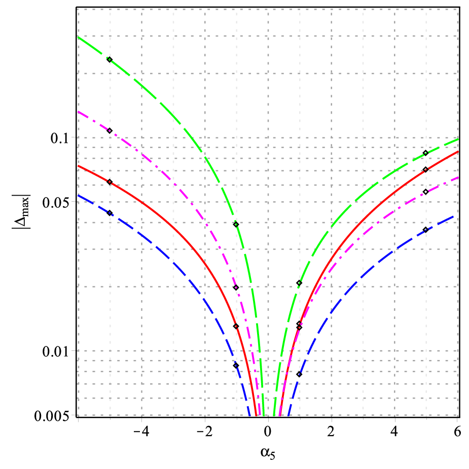
This quantity varies as a function of radius for each star, and also depends on the corresponding central density. In Fig. 7, we have plotted the quantity as a function of (where the subscript refers to the maximum value for a given choice of parameters) for the SLy, polytropic and quark star equations of state.
A necessary condition for the validity of the perturbative approach is . The plots for the SLy and polytropic equations of state (left and middle) show that the model can be treated pertubatively for . The dependence of on is linear, with the slope depending on the value of . Including a small logarithmic term () decreases , however, increasing further leads to larger deviations from GR and thus larger values of . As mentioned above, in the quark star case, we can reach larger values of respect to neutron stars while remaining in the the perturbative regime.
 |
 |
 |
V Summary
In this article we have considered the effect of a logarithmic theory, , motivated by the form of the one-loop effective action arising from gluons in curved spacetime, on the structure of relativistic stars. Unlike many theories in the literature, the modifications to General Relativity are significant in the strong-field regime, which is less well constrained by observations. Considering the motivation, we treat the model as an effective theory, valid in the interior and near vicinity of neutron stars, where QCD effects play an important role.
An theory inevitably introduces a scalar degree of freedom, and in Section III.1 we have derived the constraints imposed upon the parameters of the model due to stability and internal consistency requirements. Unlike the related model, we find that, when the logarithmic term is a subdominant correction — i.e. , which we assume throughout this work — one can consider positive and negative values of . In addition, in the absence of matter, the existence of a stable minimum at forces us to work with negative values of the coefficient of the logarithmic term .
In Section III.2, we have also considered the constraints imposed upon the model by observations; in particular relating to the possibility of a fifth force due to the scalar degree of freedom. Since we treat the model as an effective theory valid only in the vicinity of ultra-dense matter, we do not need to contend with cosmological or terrestrial constraints, however, it is important to consider the effect of the modification on binary pulsars and direct observations of neutron stars. Transforming the theory to the Einstein frame, we have shown that the model exhibits a chameleon effect, completely suppressing the effect of the modification on scales exceeding a few radii, so that any effect on the orbital motion of a binary system is completely negligible. We showed that this model satisfies the binary star observations of the effective gravitational constant for a wide range of parameters and .
On smaller scales, near the surface of the neutron star, the deviation from General Relativity can be significant. Observations of bursting neutron stars depend strongly on the surface redshift , which determines the shift in absorption (or emission) lines due to elements in the atmosphere, as well as the Eddington critical luminosity. In Fig. 3 we have plotted the dependence of on the radial coordinate in the immediate vicinity of the neutron star surface (which is directly related to the observable quantity ) showing that there are strong -dependent deviations from General Relativity, which could in principle be detected, utilising data from future X-ray missions.
In section IV, we have used the method of perturbative constraints to derive and solve the modified Tolman-Oppenheimer-Volkov equations for neutron and quark stars. The changes to the mass-radius diagram for neutron stars are shown in Fig. 4 for a toy polytropic equation of state and in Fig. 5 for a realistic SLy equation of state. As in the model [17, 18] there is an inversion of the modified gravity effect near the central density for the SLy equation of state. For the SLy equation of state, the deviation from GR is more evident for smaller central densities (corresponding to the lower-right of the plots in Fig. 5). However, in the polytropic case, for higher central densities (top-left part of the plots in Fig. 4) one can observe a larger deviation from GR with respect to lower central densities (bottom-right on the plots). In addition, in the polytropic case, the deviation from GR is much larger than the SLy case for equal values of the parameter . For the polytropic equation of state, the asymmetry in the M-R diagram for positive and negative values of parameter is also reduced.
As has been noted in the case of other models, there is a degeneracy with the choice of equation of state that is largely unconstrained. To break this degeneracy, one could consider other observables, such as those relating to the cooling [67] or spin properties [68] of the neutron stars. In particular, it was suggested in [16] that since cooling by neutron emission — which is the dominant cooling mechanism for young ( years) neutron stars — is particularly sensitive to the central density of the star, measurements of the surface temperature could offer a discriminant. However, in practice, the neutrino cooling rate is difficult to model due to the strong dependence on features such as condensates in the star’s composition.
We find that the range of the parameter that is consistent with the perturbative treatment in our model for the SLy and polytropic equations of state is comparable with that in related works, where [17, 23], [18]. In the quark star case, one can reach larger values of while remaining in the the perturbative regime.
Finally, in section IV.4, we have considered the case of self-bound stars, consisting of strange quark matter. We found that the - diagram and internal density distribution were insensitive to the presence of the logarithmic term, and for positive the mass is always enhanced relative to that calculated using General Relativity.
As the modified Tolman-Oppenheimer-Volkov equations for the model considered here involve terms that are not well defined at we have restricted our analysis to the domain. Since neutron star equations of state are stiff and , when we cannot consider central densities above a maximum value. This is particularly evident in Fig. 5, as the largest deviations from GR occur for stars with low masses, corresponding to a medium central density. Using an equation of state that is less stiff for large densities would give rise to more significant deviations for larger mass stars. This can be seen in the quark star case.
To conclude, we have shown that considering the finite logarithmic terms arising in the calculation of the effective action for a gauge field in a phenomenological framework leads to interesting observational consequences differing from the predictions of General Relativity. To make this connection more definite is beyond the scope of this article, although as observational data improve, one can entertain the possibility that neutron star systems may in the future have a role to play in analysing the predictions of quantum field theory in curved spacetime.
Acknowledgements
We would like to thank F. R. Klinkhamer, C. Rahmede, V. Emelyanov, J. Creighton and Y. Ekşi for helpful and useful discussions and comments. The work of JMW is supported by the “Helmholtz Alliance for Astroparticle Physics HAP”, funded by the Initiative and Networking Fund of the Helmholtz Association.
References
References
- [1] A. S. Eddington, Mathematical Theory of Relativity (Cambridge University Press, Cambridge, 1923).
- [2] H. Weyl, Annalen der Physik 364, 101 (1919).
- [3] A. Starobinsky, Physics Letters B 91, 99 (1980).
- [4] A. G. Riess et al. (Supernova Search Team), Astron.J. 116, 1009 (1998), arXiv:astro-ph/9805201 [astro-ph] .
- [5] S. Perlmutter et al. (Supernova Cosmology Project), Astrophys. J. 517, 565 (1999), arXiv:astro-ph/9812133 [astro-ph] .
- [6] T. P. Sotiriou and V. Faraoni, Rev.Mod.Phys. 82, 451 (2010), arXiv:0805.1726 [gr-qc] .
- [7] A. De Felice and S. Tsujikawa, Living Reviews in Relativity 13, 3 (2010), arXiv:1002.4928 [gr-qc] .
- [8] J. Khoury and A. Weltman, Phys. Rev. Lett. 93, 171104 (2004a), arXiv:astro-ph/0309300 [astro-ph] .
- [9] J. Khoury and A. Weltman, Phys. Rev. D69, 044026 (2004b), arXiv:astro-ph/0309411 [astro-ph] .
- [10] P. Brax, C. van de Bruck, A.-C. Davis, and D. J. Shaw, Phys. Rev. D78, 104021 (2008), arXiv:0806.3415 [astro-ph] .
- [11] D. Psaltis, Living Reviews in Relativity 11 (2008a), arXiv:0806.1531 [astro-ph] .
- [12] T. Kobayashi and K.-i. Maeda, Phys.Rev. D78, 064019 (2008), arXiv:0807.2503 [astro-ph] .
- [13] A. Upadhye and W. Hu, Phys.Rev. D80, 064002 (2009), arXiv:0905.4055 [astro-ph.CO] .
- [14] E. Babichev and D. Langlois, Phys.Rev. D81, 124051 (2010), arXiv:0911.1297 [gr-qc] .
- [15] E. Babichev and D. Langlois, Phys.Rev. D80, 121501 (2009), arXiv:0904.1382 [gr-qc] .
- [16] A. Cooney, S. DeDeo, and D. Psaltis, Phys.Rev. D82, 064033 (2010), arXiv:0910.5480 [astro-ph.HE] .
- [17] A. S. Arapoglu, C. Deliduman, and K. Y. Eksi, JCAP 1107, 020 (2011), arXiv:1003.3179 [gr-qc] .
- [18] M. Orellana, F. Garcia, F. A. Teppa Pannia, and G. E. Romero, Gen. Relativ. Gravit. (2013), arXiv:1301.5189 [astro-ph.CO] .
- [19] C. Deliduman, K. Eksi, and V. Keles, JCAP 1205, 036 (2012), arXiv:1112.4154 [gr-qc] .
- [20] E. Santos, Astrophys. Space Sci. 341, 411 (2012), arXiv:1104.2140 [gr-qc] .
- [21] F. Kamiab and N. Afshordi, Phys. Rev. D84, 063011 (2011), arXiv:1104.5704 [astro-ph.CO] .
- [22] E. Santos, Phys.Rev. D81, 064030 (2010), arXiv:0909.0120 [gr-qc] .
- [23] M.-K. Cheoun, C. Deliduman, C. Güngör, V. Keleş, C. Ryu, et al., (2013), arXiv:1304.1871 [astro-ph.HE] .
- [24] S. Capozziello, M. De Laurentis, S. Odintsov, and A. Stabile, Phys.Rev. D83, 064004 (2011), arXiv:1101.0219 [gr-qc] .
- [25] S. Capozziello, M. De Laurentis, I. De Martino, M. Formisano, and S. Odintsov, Phys.Rev. D85, 044022 (2012), arXiv:1112.0761 [gr-qc] .
- [26] K. Bamba, S. Nojiri, and S. D. Odintsov, Phys.Lett. B698, 451 (2011), arXiv:1101.2820 [gr-qc] .
- [27] A. Borisov, B. Jain, and P. Zhang, Phys.Rev. D85, 063518 (2012), arXiv:1102.4839 [astro-ph.CO] .
- [28] L. Reverberi, Phys. Rev. D 87, 084005 (2013), 10.1103/PhysRevD.87.084005, arXiv:1212.2870 [gr-qc] .
- [29] M. Sharif and H. R. Kausar, Astrophys.Space Sci. 337, 805 (2012).
- [30] S. Nojiri and S. D. Odintsov, Gen. Rel. Grav. 36, 1765 (2004), arXiv:hep-th/0308176 [hep-th] .
- [31] M. B. Baibosunov, V. T. Gurovich, and U. M. Imanaliev, Soviet Journal of Experimental and Theoretical Physics 71, 636 (1990).
- [32] A. Vilenkin, Phys. Rev. D 32, 2511 (1985).
- [33] G. M. Shore, Annals of Physics 128, 376 (1980).
- [34] J.-Q. Guo and A. V. Frolov, (2013), arXiv:1305.7290 [astro-ph.CO] .
- [35] N. Birrell and P. Davies, Quantum Fields in Curved Space, Cambridge Monographs on Mathematical Physics (Cambridge University Press, 1982).
- [36] T. Leen, Annals of Physics 147, 417 (1983).
- [37] E. Calzetta, I. Jack, and L. Parker, Phys. Rev. Lett. 55, 1241 (1985).
- [38] E. Calzetta, I. Jack, and L. Parker, Phys. Rev. D 33, 953 (1986).
- [39] N. K. Nielsen and B. S. Skagerstam, Phys. Rev. D 34, 3025 (1986).
- [40] N. Itoh, Progress of Theoretical Physics 44, 291 (1970).
- [41] E. Witten, Phys. Rev. D 30, 272 (1984).
- [42] C. Alcock and A. Olinto, Ann. Rev. Nucl. Part. Sci. 38, 161 (1988).
- [43] F. Weber, A. Torres i Cuadrat, A. Ho, and P. Rosenfield, PoS JHW2005, 018 (2006), arXiv:astro-ph/0602047 [astro-ph] .
- [44] J. Lattimer and M. Prakash, Astrophys. J. 550, 426 (2001), arXiv:astro-ph/0002232 [astro-ph] .
- [45] F. Ozel, Nature 441, 1115 (2006).
- [46] L. Parker and D. Toms, Quantum field theory in curved spacetime. Quantized fields and gravity. (Cambridge Monographs on Mathematical Physics. Cambridge University Press, 2009).
- [47] A. Dolgov and M. Kawasaki, Phys. Lett. B573, 1 (2003), arXiv:astro-ph/0307285 [astro-ph] .
- [48] A. V. Frolov, Phys.Rev.Lett. 101, 061103 (2008), arXiv:0803.2500 [astro-ph] .
- [49] D. F. Mota and D. J. Shaw, Phys.Rev. D75, 063501 (2007), arXiv:hep-ph/0608078 [hep-ph] .
- [50] G. Esposito-Farese, (2004), arXiv:gr-qc/0402007 [gr-qc] .
- [51] J. M. Weisberg and J. H. Taylor, ASP Conf.Ser. (2002), arXiv:astro-ph/0211217 [astro-ph] .
- [52] M. Bailes, S. Ord, H. Knight, and A. Hotan, Astrophys. J. 595, L49 (2003), arXiv:astro-ph/0307468 [astro-ph] .
- [53] A. Wolszczan, Nature 350, 688 (1991).
- [54] T. Damour and G. Esposito-Farese, Phys. Rev. D58, 042001 (1998), arXiv:gr-qc/9803031 [gr-qc] .
- [55] J. Naf and P. Jetzer, Phys.Rev. D84, 024027 (2011), arXiv:1104.2200 [gr-qc] .
- [56] S. DeDeo and D. Psaltis, Phys. Rev. Lett. 90, 141101 (2003), arXiv:astro-ph/0302095 [astro-ph] .
- [57] D. Psaltis, Phys. Rev. D77, 064006 (2008b), arXiv:0704.2426 [astro-ph] .
- [58] H. A. Buchdahl, Phys.Rev. 116, 1027 (1959).
- [59] F. Özel, Rept. Prog. Phys. 76, 016901 (2013), arXiv:1210.0916 [astro-ph.HE] .
- [60] X. Barcons, D. Barret, A. Decourchelle, J.-W. Herder, T. Dotani, et al., (2012), arXiv:1207.2745 [astro-ph.HE] .
- [61] J. R. Oppenheimer and G. M. Volkoff, Phys. Rev. 55, 374 (1939).
- [62] A. W. Steiner, J. M. Lattimer, and E. F. Brown, Astrophys.J. 722, 33 (2010), arXiv:1005.0811 [astro-ph.HE] .
- [63] P. Haensel and A. Y. Potekhin, Astron. Astrophys. 428, 191 (2004), arXiv:astro-ph/0408324 [astro-ph] .
- [64] F. Ozel, G. Baym, and T. Guver, Phys.Rev. D82, 101301 (2010), arXiv:1002.3153 [astro-ph.HE] .
- [65] C. Alcock, E. Farhi, and A. Olinto, Astrophys. J. 310, 261 (1986).
- [66] N. Stergioulas, Living Rev.Rel. 6, 3 (2003), arXiv:gr-qc/0302034 [gr-qc] .
- [67] D. Page, U. Geppert, and F. Weber, Nucl.Phys. A777, 497 (2006), arXiv:astro-ph/0508056 [astro-ph] .
- [68] M. Baubock, E. Berti, D. Psaltis, and F. Özel, (2013), arXiv:1306.0569 [astro-ph.HE] .