Thermal Instability behind a Shock Wave in HI and Molecular CloudsNote: Not to appear in Nonlearned J., 45.
Abstract
We performed one-dimensional hydrodynamic simulations with detailed cooling, heating and chemical processes to examine the thermal stability of shocked gas in cold neutral medium (CNM) and molecular clouds. We find that both CNM and molecular clouds can be thermally unstable in the cooling layer behind the shock wave. The characteristic wavelength of the thermal instability ranges from pc to pc in the CNM, and from pc to pc in the molecular clouds. This coincides with the size of observed tiny scale structures in the CNM and molecular clouds, indicating that the thermal instability in the shocked gas could be a formation mechanism of these tiny structures in the interstellar medium. We have also calculated the -folding number of the thermal instability to estimate the amplification of the density fluctuation in the shocked gas. Density perturbations in the CNM grow by a factor of exp(5), whereas the perturbations in the molecular clouds grow only by a factor of a few behind a high Mach number shock. The amplification factor is larger at lower densities and higher velocities. Formation of very small-scale structures by thermal instability in shocked gas is more effective in lower densities.
Keywords:
ISM: clouds – ISM: molecules – ISM: structure – Shock wavesI Introduction
Thermal instability is an important physical process to determine the structure in the interstellar medium [8]. It is well established that the neutral gas in the interstellar medium (ISM) consists of two distinct phases: cold neutral medium (CNM) and warm neutral medium (WNM) (e.g., Field, Goldsmith & Habing 9; Wolfire et al. 63, Heiles & Troland 22). [9] calculated the thermal equilibrium state in ISM considering the cosmic ray heating and line cooling by H, O, and C[II]. They showed that there are three physical states under the pressure equilibrium: two stable states and one unstable state. The stable states correspond to the CNM and the WNM. When the WNM transforms to the CNM in converging flows and/or shocks, the gas goes through a thermally unstable state (e.g., Hennebelle & Pérault 29, Koyama & Inutsuka 39; Heitsch et al. 26, Vázquez-Semadeni et al. 60).
Many authors have studied the dynamical condensation and fragmentation processes of the ISM driven by the thermal instability in the shock in WNM. [39, 40] showed that small-scale clumps of CNM are formed behind the shock front in WNM (see also, Hennebelle & Pérault 29, Hennebelle & Audit 27, Inoue & Inutsuka 35, Inoue & Inutsuka 36, Heitsch et al. 25, Vázquez-Semadeni et al. 59). [39] also investigated the shock propagation within the CNM, and found that the shocked layer in the CNM is thermally unstable, as well. More recently, Inoue & Inutsuka [37] has succeeded in forming very turbulent molecular clouds by accretion of CNM mixed with WNM.
The thermal instability works as follows. Consider an isobaric gas with small density perturbation. If the gas in small density enhancement (i.e. temperature decline) has a larger cooling rate than the surrounding gas, the density enhancement grows. In other words, the condition is determined by how the cooling rate depends on the density and temperature. Thermal instability thus could occur in denser regions like molecular clouds as well, and has actually been studied. [5] investigated the thermal-chemical instability (e.g., Glassgold & Langer 15) in the chemical transition region where the dominant form of carbon changes from C[II] to CO (Glassgold & Langer 14), and showed that the thermal-chemical instability is not active. [13] investigated thermal instability in molecular clouds with density cm-3 and temperature - , and found that such a cloud is thermally unstable. [48, 49] investigated thermal instability in molecular cloud cores ( cm-3) with the effect of the ambipolar diffusion, and showed that the thermal instability can grow in quasi-magnetohydrostatic, self-gravitating slab (Nejad-Asghar 48) and axisymmetric cylindrical core (Nejad-Asghar 49).
On the other hand, to our best knowledge, the role of thermal instability in shock heated molecular clouds has not yet been studied. Molecular clouds are characterized by supersonic velocity dispersions, which are most probably due to turbulence (Larson 42, Solomon et al. 53). Dissipation of the supersonic turbulence would be accompanied by shocks. Shock waves are also driven by collisions of protostellar outflows with ambient gas.
Molecular clouds are known to have clumpy structures. While many of the clumps are gravitationally bound, there are very small-scale structures as well: a size of 1000AU and density of cm-3 [41, 24, 51, 56]. Since they are gravitationally unbound (), they cannot be formed by gravitational instability. Although shock compression by turbulence often makes gravitationally unbound structure, it would not be easy to make very small-scale structure ( pc) by shock compression alone. Firstly, the shock compresses the gas as a whole, and thus cannot make fragments. Since turbulence has eddies of various spatial scales, one may imagine that the shock compression at small scale eddied can make very small-scale structures or fragments. But it should be noted that the turbulence (i.e. velocity dispersion in molecular clouds) becomes subsonic at 0.1 pc according to Larson’s law (see e.g., Heyer & Brunt 31). Structures smaller than this scale thus cannot be formed by shock compression by turbulence. If the shocked molecular gas is thermally unstable, it could generate very small-scale fragments. The effect of thermal instability on the shocked molecular gas must be explored.
In this paper, we examine the thermal stability of shocked gas in molecular clouds using one-dimensional hydrodynamic simulations including detailed cooling, heating and chemical processes. Although our main target is molecular clouds, we also calculate one model of CNM, in order to compare our results with Koyama & Inutsuka [39], and to compare the e-folding numbers in CNM and molecular clouds. This paper is organized as follows. In §2, we describe our physical and chemical models. Then, we explain the condition for the thermal instability and how we evaluate the growth of perturbation in §3. In §4, we show the results of our simulations of shock propagation in CNM and molecular clouds. Finally, we summarize our results in §5.
II The model
We investigate the evolution of ISM swept by a shock wave in a plane-parallel gas. Figure 1 schematically shows the configuration of our model; we consider a collision of oppositely oriented gas flows which have the same density, temperature and chemical composition. The external radiation irradiates both ends of the numerical domain. We calculate the temporal variation of temperature, density, and chemical composition in the shocked region.
II.1 Basic Equations
We solve the following equations:
where , , and are the gas mass density, velocity, thermal pressure, ratio of specific heat, heating and cooling rate per unit mass, respectively. We use an operator-splitting technique to solve these equations, which are split into three parts: (1) ideal hydrodynamics, (2) cooling and heating, and (3) chemical reactions (e.g., Inoue & Inutsuka 35). The first part, ideal hydrodynamics, is calculated by employing a second-order Godunov method with Lagrangian coordinates [61]. We solve the exact Riemann problem iteratively at each grid cell interface to calculate numerical fluxes, and determine the position of grid cell interface in the next time step. Thus, we can appropriately calculate small-scale compressed dense regions and large-scale pre-shock regions at once. The energy equation
is solved by the second-order explicit method. Temporal variation of the number density of chemical species is determined by the rate equations
where is the rate coefficient of the chemical reactions. The rate equations are calculated by a first-order implicit method [30].
The time step of the integration is set to be small enough to satisfy the CFL condition, and to be much smaller ( %) than the cooling time scale of the gas. The details of the physical and chemical processes considered in our model are described in the following.
II.2 Heating and Cooling Processes
A full list of the thermal processes included in our model is listed in Table 1. Our model includes the cooling by the line emission of H, C[II], O[I], and CO with the effect of radiative trapping, recombination on grains, and dust-gas collision. We adopt the formula of escape probability by [5] for the line cooling by C[II] and O[I], and by [32] for CO. The escape probability is a function of the column density of the molecule or atom ; the number density is integrated from the edge of the numerical domain to the center of each grid cell. Since our model is 1D, we calculate the escape probabilities towards the right-hand-side and left-hand-side edges of the numerical domain, and use the average of these two values. Gas is also cooled by collisions with dust; the dust temperature is set to 10K (e.g., section 5 of Tielens 57). Heating processes include photo-electric heating by PAH [1], cosmic ray [17], and H2 photo-dissociation [4]. In the calculation of photo-electric heating, we consider the attenuation of external radiation. Visual extinction, , is calculated by
where the numerator is the column density of hydrogen nuclei integrated from the edge of the numerical domain to the center of each grid cell (e.g., Mathis et al. 45).
II.3 Chemical reactions
We calculate the chemical reaction network in the gas phase, which consists of 462 species and 9578 reactions.
Chemical reactions and rate coefficients are adopted mainly from OSU network
(http://www.physics.ohio-state.edu/~eric), which is developed for interstellar chemistry.
Namely, we use the network of [12] at K
and [19] (see also Harada et al. 20, the errata of Harada et al. 19) at K.
These networks contain cosmic ray ionization, ion-molecule reactions, neutral-neutral reactions, recombination of ion,
photo reactions, and grain surface reactions.
We also include the collisional dissociations in Table A1 of [62],
but some rate coefficients are modified (see the appendix of Furuya et al. 11).
We do not consider grain-surface reactions except for H2 formation.
Cosmic-ray ionization rate is set to be 1.3 s-1.
In the model of CNM gas, the total column density of hydrogen nuclei is only cm-2,
and the molecules are destroyed by photo reactions.
We take into account the self-shielding effects of H2, CO and C atom referring to [43] and [58];
the shielding factors are given as a function of and the column densities of specific species integrated from
the edges of the numerical domain to each grid cell at every time step.
Elemental abundances in the gas phase are listed in Table 2.
II.4 Initial and Boundary conditions
The initial temperature and chemical composition of the colliding gases are determined by calculating the thermal and chemical equilibrium. In the model of CNM, these initial conditions vary spatially depending on the visual extinction at each position in the numerical domain. In the model of molecular clouds, is set to be 5 mag for all grid cells; our numerical domain is an embedded small portion of the molecular cloud. In total, we calculate one CNM model and 45 molecular cloud models. The model parameters are summarized in Table 3.
Our initial condition of the CNM is basically the same as that of Koyama & Inutsuka [39] (see their §3.4); we assume the number density to be cm-3. Thermal equilibrium determines the gas temperature, which is about 110 K at any position. The velocity of the colliding gas (see Figure 1) is 10km/s, which corresponds to the velocity of gas flow associated with old supernova remnants. Total column density of hydrogen nuclei is set to be cm-2, i.e. mag.
For the molecular cloud models, we explore the parameter space of the number density : , , , and cm-3. The velocity ranges from 0.5 to 4.5 km s-1, referring to the turbulent velocities in molecular clouds [42, 10]. We also investigate a model with km s-1, which is a typical velocity of protostellar outflows (e.g., Moriarty-Schieven & Snell 47).
In the model of the CNM, the size of our numerical domain is 3.24 pc, which covers the whole region of the CNM. In order to calculate the post-shock region with a high spatial resolution, we set 225 grid cells at , and 35 grid cells at (see Figure 1). Initially, is 0.972 pc. Both and change with time, since we are using Lagrangian coordinates. In the models of molecular clouds, our numerical domain varies from 0.01 pc to 0.28 pc depending on the model parameters (see Table 3). The numerical domain is divided into 300 grid cells with equal intervals.
We adopt the free-boundary condition;
i.e. we assume that the physical values of left and right side of boundary are the same when we solve the exact Riemann problem at boundary. Basically, the boundary condition is not important, because we stop the calculation before the shock wave reaches the boundary.
III Amplitude of thermal instability
[2] showed that for any unperturbed state, the gas is thermally unstable if
| (1) |
where is specific entropy, is temperature, and is a thermodynamic variable kept constant in the perturbation. Since the ISM is mostly in pressure equilibrium, the isobaric condition, , is satisfied, which leads to
| (2) |
[52] and [39] performed a linear analysis of thermal instability in isochorically cooling gas and isobarically contracting gas, respectively. When the gas is thermally unstable, the density perturbation grows as . The growth rate in isobarically contracting gas is
| (3) | |||||
where is the mean molecular mass, and and are the cooling and heating time scales, respectively. is a function of density and temperature, that changes with time as the gas goes through the shock wave and enters the cooling region. When the gas is thermally unstable, takes a positive value.
In this paper, we evaluate the integrated -folding number as an indicator of the amplification of the perturbation, where the -folding number is calculated for each fluid element in Lagrangian coordinate, and the integral is executed only when the Balbus criterion (Eq 1) is satisfied. Then, using the -folding number, we obtain the amplification of the thermal instability .
In the linear analysis, the growth rate is a function of the wavelength of the perturbation, and Eq. (3) is the rate for the most unstable mode at
| (4) |
The Field length is
| (5) |
where the thermal conductivity is 2.5 cm-1 K-1 s-1 [50]. The acoustic length is
| (6) |
where is the sound speed, is the specific internal energy, and is the net cooling time scale [8]. It should be noted, however, that the dependence of the growth rate on perturbation wavelength is considerably weak around the most unstable wavelength. The growth rate is comparable to equation (3) in the wavelength range of
| (7) |
(Field 8, see also Appendix B of Koyama & Inutsuka 39).
Ideally, the growth of density perturbation should be measured in hydrodynamic simulations starting from an initial condition with small amplitude perturbations. But it is not easy in practice. First of all, the thickness of the unstable layer is comparable to or smaller than the most unstable wavelength (see Figure 3). In one dimensional flow, the perturbation grows as long as Eq. (1) is satisfied, but when the gas is compressed to be in thermally stable state, the perturbation is dispersed, which is an artifact. In 2D and/or 3D simulations, large scale perturbations up to the acoustic length can grow in directions parallel to the shock front, and these clump structures remain in the post-shock regions (e.g., Inoue & Inutsuka 35). The 2D/3D simulation is, however, very time consuming, especially if we are to resolve the perturbations with very small wavelengths. It is well established that the growth rate derived from the linear analysis is applicable to non-linear regime of thermal instability. For instance, we can see in Figure 1 of [38] that the isobaric condition, which is required for the thermal instability to grow with the linear growth rate, is met throughout the evolution without interceptive feedback effects. Therefore, it is reasonable to estimate the amplification of the density perturbation by integrating the e-folding number along the 1D flow. It should at least be done before investing a large computational time on 2D hydrodynamic simulation with perturbation and very high spatial resolution. We also note here that our present work is analogous to [39]; they performed 1D shock calculation to find that the gas becomes thermally unstable in the shock-compressed layer and predicted that small clumps would be formed. Later, [40] indeed showed that such clumps are formed in the 2D simulation.
IV Results
We have calculated the generation and propagation of shock waves in CNM and molecular clouds by solving the basic equations in §2.1. In the following, we show the spatial distribution of physical parameters and the e-folding number when the shock wave reaches a steady state.
IV.1 Shock Propagation in CNM
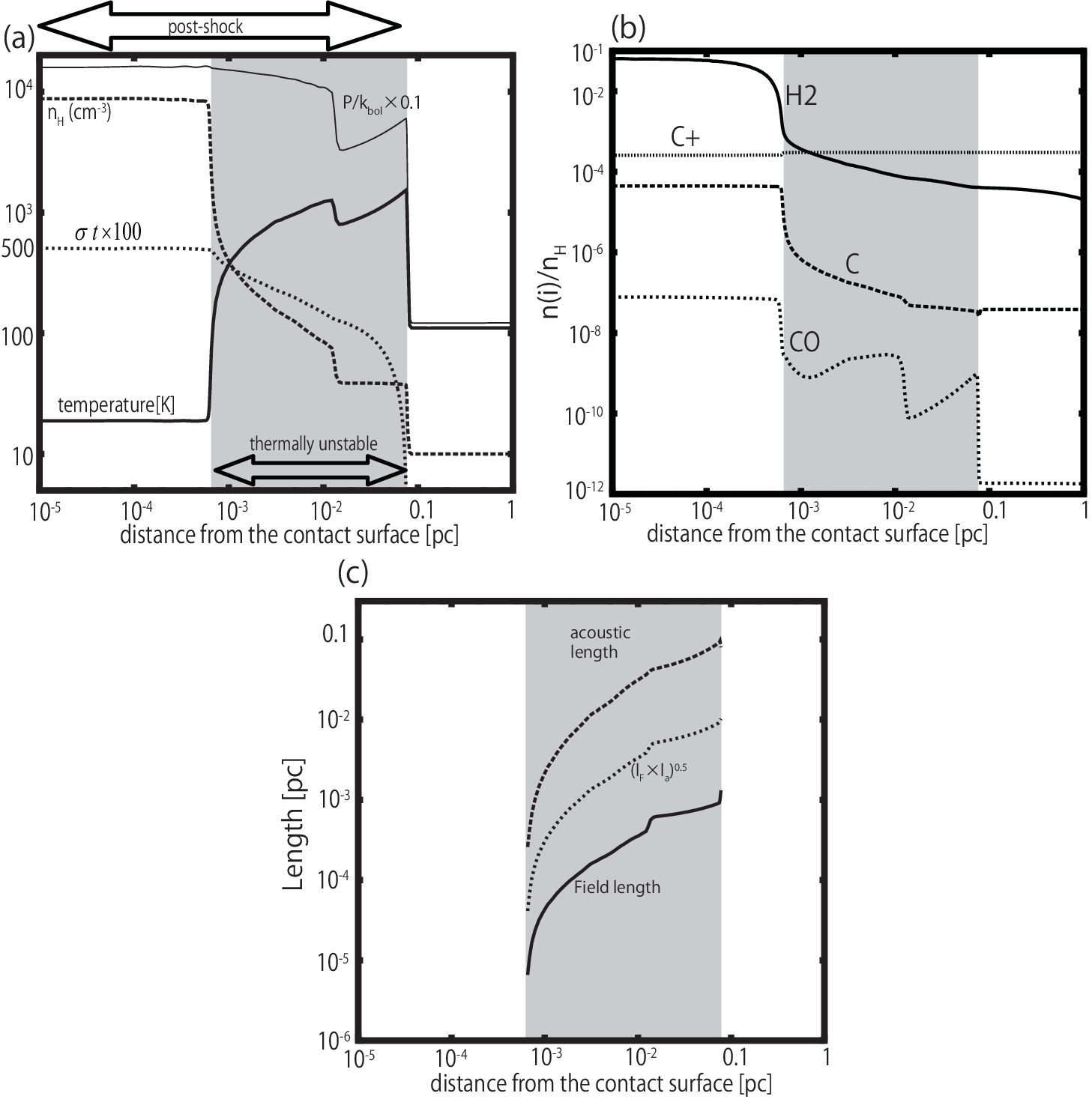
Figure 2 (a) shows the distribution of temperature, number density of hydrogen nuclei (), thermal pressure, and integrated -folding number at yr in the CNM model. A similar simulation was performed by [39]. Temperature and density distributions in Figure 2 are indeed similar to Figure 7 of [39], who found that the shocked CNM evolves through a thermally unstable state. The gray shade in Figure 2 depicts the thermally unstable region, in which the condition (1) is satisfied. CNM becomes thermally unstable immediately behind the shock and then evolves to a thermally stable dense gas with basically isobaric condition (see Figure 7 (a) of Koyama & Inutsuka 39). The main coolants are CII(158m) and OI(63m). Now, we go one step further from [39] and calculate the e-folding number. The integrated -folding number is approximately 5, which means that the density fluctuation grows by a factor of exp(5). Note that the density profile shown in Figure 2 is the unperturbed value. For example, if the pre-shock gas has a density fluctuation of 10, i.e. 11 cm-3 in the pre-shock gas of 10 cm-3, the fluctuation grows by a factor of 150, 1.6 104 cm-3 in the post-shock gas of 1.0 103 cm-3.
We also show the distribution of assorted chemical species (Figure 2 ). Molecular hydrogen in the pre-shock region in our model is more abundant than that of [39] due to the difference in the self-shielding model; [39] used the formulation by [58], while we use the Table 10 in [43]. In the dense stable region ( pc), on the other hand, the H2 abundance in our model is almost the same as that in [39]. H2 is formed by the association of H atoms on grain surfaces and destroyed by photo-dissociation. Figure 2 (b) also shows the abundances of C+, C and CO. Although [39] did not show the spatial distribution of CO, they reported that 0.02 % of the carbon is in CO in the dense stable gas in the post-shock region. In our model 0.03 % of carbon is in CO. It should be noted that we solve the detailed chemical network, whereas [39] adopted a simplified chemical model that assumed a direct conversion of C+ to CO without accounting explicitly for the intermediate reactions. Consistency of our model results with [39] validates their simplified model.
Figure 2 (c) shows the Field length, acoustic length and the most unstable wavelength of perturbation in the unstable region. The Field length is pc and the acoustic length is pc. The most unstable wavelength ranges from to pc, which coincides with the size of the tiny scale structures observed in CNM, pc (see Table 1 of Heiles 21). Such tiny structures can be formed by thermal instability [39].
IV.2 Shock Propagation in Molecular Clouds
Figure 3 (a) shows the spatial distribution of temperature, number density of hydrogen nuclei (), thermal pressure, and integrated -folding number in the model with 4.5 km s-1 and a pre-shock density cm-3 at yr. The gas becomes thermally unstable immediately behind the shock, where the gas temperature reaches near 1000 K. The gas evolves in the post-shock region with the isobaric condition. The main coolant is CO in this warm gas. The integrated -folding number is 1.25; if we calculate the HD simulation with a small perturbation, it grows only by a factor of 3.5.
Figure 3 (b), on the other hand, shows a model with a higher initial density cm-3 at yr. In this model, the post-shock gas becomes thermally unstable right behind the shock front, but then becomes stable, although the temperature (several hundreds of K) in this region is similar to that in the unstable post-shock gas in Figure 3 (a). Once the number density reaches several times 105 cm-3, the dust-gas collisional cooling becomes dominant and the gas becomes thermally unstable again. The integrated -folding number is even smaller than in the model of Figure 3 (a).
Figure 3 (c) and (d) show the spatial distribution of the Field length, acoustic length and the most unstable wavelength in the two models of molecular gas. In the model with higher gas density, the cooling rate is higher (see below), and thus these scale lengths become shorter (see Eq (5) and (6)).
We summarize the integrated -folding number in our molecular cloud models in Table 4. We can see that the shocked molecular gas is unstable when is larger than km s-1, and that the integrated -folding number increases with increasing and decreasing initial gas density. These dependences can be understood as follows. When the net cooling rate per unit mass is proportional to , the criterion for thermal instability by [2] can be rewritten as (see Appendix A). The gas is more unstable when is larger and is smaller. In other words, the perturbation grows faster when the dependence of the cooling rate on the temperature is weaker and/or dependence of the cooling rate on gas density is stronger. The cooling rate actually is a more complicated function of density and temperature than a power law . But we can define and as a local tangent in logarithmic plot. Figures 4 (a) and (b) show the local tangent, and , of the cooling rate by CO rotational lines as a function of temperature and density at a typical molecular cloud condition. We can see that is larger at lower densities and is larger at low temperatures. In general, when the gas temperature is high enough to excite the coolant species (e.g., C+, CO), the cooling rate does not significantly decrease as the temperature is lowered. When the gas temperature is comparable to the upper state energy of the line, on the other hand, the cooling rate decreases steeply as the gas temperature is lowered. The dependence of on density can be understood by considering the critical density, which is cm-3 for CO rotational lines [46]. When the gas density is much smaller than the critical density, the cooling rate per unit volume is proportional to , whereas at the critical density or higher, the dependence is weaker than because of collisional de-excitation (see e.g., section 2.3.1 of Tielens 57).
In Table 4, asterisks indicate that the dust-gas collisional cooling dominates over the CO cooling in the model. The cooling rate by dust-gas collision per unit mass is given as
where is the mean molecular mass and we set Å and K [33]. It is obvious that is always 1 in any density region, and that dust-gas collisional cooling is important at high densities. Figure 4 (c) shows the power index . The cooling rate is proportional to when , but becomes larger than 1.5 when (see Appendix B). Since the dust temperature is 10 K in our model, the gas is more unstable at higher temperatures.
V Summary and Discussion
We performed the one-dimensional hydrodynamic simulations with the effects of heating, cooling and chemical reactions in order to study the thermal stability of shocked gas in CNM and molecular clouds. Taking advantage of the fact that the growth rate derived from the linear analysis [52, 39] is applicable to the non-linear regime in thermal instability, we calculate the -folding number along the flow to evaluate the amplification of density perturbation behind the shock wave. Our findings are as follows
- •
Both CNM and molecular cloud can be thermally unstable behind a shock wave.
- •
A molecular cloud becomes thermally unstable behind a shock when km s-1.
- •
The integrated -folding number in the shocked molecular cloud increases with increasing and decreasing pre-shock density.
- •
The wavelength, , the perturbation of which can grow within the cooling time scale, ranges from pc to pc in the CNM, and from pc to in molecular clouds. The unstable wavelength is a decreasing function of pre-shock density and fluid velocity, since both the Field length and acoustic length scale decrease with gas density.
The unstable wavelength of the thermal instability coincides with the size of the tiny scale structures observed in the CNM [21, 55] and molecular clouds [41, 24, 51, 56]. Thermal instability could thus explain the formation of such small gravitationally-unbound clumps in the ISM. In the CNM, the initial perturbation is amplified by a factor of in the thermally unstable region behind a shock. In molecular clouds, on the other hand, the initial perturbation is amplified only by a factor of a few. It should be noted, however, that the super-sonic velocity dispersion is ubiquitous in molecular clouds. Small clumps would be formed if the molecular cloud is swept by multiple shocks.
Finally, we discuss the fate of the structure formed by the thermal instability. In the HI medium, the CNM can coexist with the WNM thanks to the thermally bistable nature (Field, Goldsmith & Habing 9). If the molecular clouds are isothermal uni-phase medium, the density fluctuations enhanced by the thermal instability could exist only in the very narrow shock transition layer, because the post-shock gas eventually returns to the same temperature as the pre-shock gas. However, recent numerical simulations of molecular cloud formation (e.g., Banerjee et al. 3, Inoue & Inutsuka 37) have shown that molecular clouds are composed of the cold molecular gas ( K and 100 cm-3) and the non-equilibrium diffuse warm gas ( K and 1 cm-3). The diffuse warm component, which is generated by the cloud-forming shocks at the envelope of molecular cloud, is in high pressure and thermally unstable. The implication of this result is twofold. Firstly, it shows that a bistability of thermal equilibrium gas is not needed for density fluctuations to survive in post shock gas. Secondly, in such a ”non-equilibrium two-phase medium”, the structure formed by the thermal instability behind the shock within molecular clouds would be more likely to survive in the non-equilibrium diffuse gas. If the perturbed gas can fragment and coexist with the diffuse gas, the very small-scale structure could survive until at least the diffuse gas cools down ( Myr). But it is still an open question, and multi-dimensional simulations are necessary to confirm our expectation.
Appendix A Modification of Balbus criterion
We assume a gas with the cooling rate (cf. Elmegreen 6). The number density and temperature of an unperturbed state are and . Then the gas is compressed isobarically; the perturbed gas density and temperatures are () and . Balbus criterion becomes
Considering , and , it is straightforward to derive
We can see that the Balbus criterion is satisfied if .
Appendix B Temperature dependence of dust-gas collisional cooling
The cooling function of dust-gas collisional cooling is
| (B1) |
where is constant, and and are temperatures of gas and dust, respectively. The power index becomes
| (B2) |
where . We set , and it is straightforward to derive
| (B3) |
If (), and if (), becomes larger than 1.5.
References
- [1] Bakes, E.L.O., & Tielens, A.G.G.M. 1994 ApJ, 427, 822
- [2] Balbus, S.A. 1986, ApJ, 303, L79
- [3] Banerjee, R., Vázquez-Semadeni, E., Hennebelle, P., & Klessen, R.S. 2009, MNRAS, 398, 1082
- [4] Black, J.H., & Dalgarno, A. 1977, ApJS, 34, 405
- [5] de Jong, T., Dalgarno, A., & Boland, W. 1980, A&A, 91, 68
- [6] Elmegreen, B.G. 1991, in The Physics of Star Formation and Early Stellar Evolution, ed. C.J. Lada & N. D. Kylafis (NATO ASI Ser. C, 342; Dordrecht:Kluwer), 35
- [7] Elmegreen, B.G., & Scalo, J. 2004, ARA&A, 42, 211
- [8] Field, G.B. 1965, ApJ, 142, 531
- [9] Field, G.B., Goldsmith, D.W., & Habing, H.J. 1969, ApJ, 155, L149
- [10] Fukui, Y., Kawamura, A., Minamidani, T. et al. 2008, ApJS, 178, 56
- [11] Furuya, K., Aikawa, Y., Tomida, K. et al. 2012, ApJ, 758, 86
- [12] Garrod, R.T., & Herbst, E., 2006, A&A, 457, 927
- [13] Gilden, D.L. 1984, ApJ, 283, 679
- [14] Glassgold, A.E., & Langer, W.D. 1975, ApJ, 197, 347
- [15] Glassgold, A.E., & Langer, W.D. 1976, ApJ, 204, 403
- [16] Glover, S.C.O., Mac Low, M-M. 2007, ApJS, 169, 239
- [17] Goldsmith, P.F., & Langer, W.D. 1978, ApJ, 222, 881
- [18] Habing, H.J. 1968, Bull. Astron. Inst. Netherlands, 19, 421
- [19] Harada, N., Herbst, E. & Wakelam, V., 2010, ApJ, 721, 1570
- [20] Harada, N., Herbst, E. & Wakelam, V., 2012, ApJ, 756, 104
- [21] Heiles, C. 1997, ApJ, 481, 193
- [22] Heiles, C., & Troland, T.H. 2003, ApJ, 586, 1067
- [23] Heiles, C., & Troland, T.H. 2005, ApJ, 624, 773
- [24] Heithausen, A. 2002, A&A, 393, L41
- [25] Heitsch, F., Hartmann, L.W., Slyz, A.D., Devriendt, J.E.G., & Burkert, A. 2008, ApJ, 674, 316
- [26] Heitsch, F., Burkert, A., Hartmann, L.W., Slyz, A.D., & Devriendt, J.E.G. 2005, ApJ, 633, L113
- [27] Hennebelle, P., & Audit, E. 2007, A&A, 465, 431
- [28] Hennebelle, P., & Falgarone, E. 2012, A&ARv, 20, 55
- [29] Hennebelle, P., & Pérault, M. 1999, A&A, 351, 309
- [30] Hersant, F., Wakelam, V., Dutrey, A., Guilloteau, S., & Herbst, E. 2009, A&A, 493, L49
- [31] Heyer, M.H., & Brunt, C.M. 2004, ApJ, 615, L45
- [32] Hollenbach, D., & McKee, C.F. 1979, ApJS, 41, 555
- [33] Hollenbach, D., & McKee, C.F. 1989, ApJ, 342, 306
- [34] Hosokawa, T., & Inutsuka, S. 2006, ApJ, 646, 240
- [35] Inoue, T. & Inutsuka, S. 2008, ApJ, 687, 303
- [36] Inoue, T. & Inutsuka, S. 2009, ApJ, 704, 161
- [37] Inoue, T. & Inutsuka, S. 2012, ApJ, 759, 35
- [38] Inoue, T., Inutsuka, S., & Koyama, H. 2007, ApJ, 658, L99
- [39] Koyama, H. & Inutsuka, S. 2000, ApJ, 532, 980
- [40] Koyama, H. & Inutsuka, S. 2002, ApJ, 564, L97
- [41] Langer, W.D., Velusamy, T., Kuiper, T.B.H. et al. 1995, ApJ, 453, 293
- [42] Larson, R.B. 1981, MNRAS, 194, 809
- [43] Lee, H.-H., Herbst, E., Pineau des Foréts, G., Roueff, E., & Le Bourlot, J. 1996, A&A, 311, 690
- [44] Mac Low, M-M., & Klessen, R.S. 2004, Rev.Mod.Phys., 76, 125
- [45] Mathis, J.S., Mezger, P.G., & Panagia, N. 1983, A&A, 128, 212
- [46] McKee, C.F., Storey, J.W.V., Watson, D.M., & Green, S. 1982, ApJ, 259, 647
- [47] Moriarty-Schieven, G.H., & Snell, R.L. 1988, ApJ, 332, 364
- [48] Nejad-Asghar, M. 2007, MNRAS, 379, 222
- [49] Nejad-Asghar, M. 2011, MNRAS, 414, 470
- [50] Parker, E.N. 1953, ApJ, 117, 431
- [51] Sakamoto, S., & Sunada, K. 2003, ApJ, 594, 340
- [52] Schwarz, J., McCray, R., & Stein, R.F. 1972, ApJ, 175, 673
- [53] Solomon, P.M., Rivolo, A.R., Barrett, J., & Yahil, A. 1987, ApJ, 319, 730
- [54] Spitzer, L. 1978, Physical Processes in the Interstellar Medium (New York:Wiley)
- [55] Stanimirović, S., & Heiles, C. 2005, ApJ, 631, 371
- [56] Tachihara, K., Saigo, K., Higuchi, A. et al. 2012, ApJ, 754, 95
- [57] Tielens, A.G.G.M. 2005, The Physics and Chemistry of the Interstellar Medium (Cambridge University Press)
- [58] Tielens, A.G.G.M., & Hollenbach, D. 1985, ApJ, 291, 722
- [59] Vázquez-Semadeni, E., Gómez, G.C., Jappsen, A.K. et al. 2007, ApJ 657, 870
- [60] Vázquez-Semadeni, E., Ryu, D., Passot, T., González, R.F., & Gazol, A. 2006, ApJ 643, 245
- [61] Van Leer, B. 1979, J. Comput. Phys., 32, 101
- [62] Willacy, K., Klahr, H.H., Millar, T.J., Henning, Th. 1998, A&A, 338, 995
- [63] Wolfire, M.G., Hollenbach, D., McKee, C.F., Tielens, A.G.G.M. & Bakes, E.L.O. 1995, ApJ, 443, 152
- [64] Wolfire, M.G., McKee, C.F., Hollenbach, D., & Tielens, A.G.G.M. 2003, ApJ, 587, 278
| Cooling & heating process | reference |
|---|---|
| Ly- cooling | [54] |
| C+ fine structure cooling(158m) | [5], [33] |
| O fine structure cooling(63m) | [5], [64] |
| CO rotational cooling | [32], [34] |
| CO vibrational cooling | [33] |
| Cooling due to recombination on grains | [1] |
| Cooling by the collision with dust | [33] |
| Photoelectric heating by PAH | [1], [64] |
| Cosmic ray heating | [17] |
| H2 photo-dissociation heating | [4] |
| element | abundance | element | abundance |
|---|---|---|---|
| He | 9.75 | Fe | 2.47 |
| O | 4.5 | Na | 2.25 |
| C | 3.02 | Mg | 1.09 |
| N | 2.47 | P | 2.16 |
| S | 9.14 | Cl | 1.0 |
| Si | 2.47 |
| nH [cm-3] | T [K] | G0 aaExternal FUV radiation normalized to the local interstellar radiation field (1.6 ergs cm-2 s-1) of [18]. | H atom bbRelative abundance of chemical species to hydrogen nuclei(). means . | H2 bbRelative abundance of chemical species to hydrogen nuclei(). means . | C atom bbRelative abundance of chemical species to hydrogen nuclei(). means . | CO bbRelative abundance of chemical species to hydrogen nuclei(). means . | C+ bbRelative abundance of chemical species to hydrogen nuclei(). means . | ccInitial numerical domain (see Figure 1). [pc] |
|---|---|---|---|---|---|---|---|---|
| CNM | ||||||||
| 10 | 110 | 1.7 | 1.0 | 2.5(-5) | 3.8(-8) | 1.8(-12) | 3.0(-4) | 3.24 |
| molecular cloud | ||||||||
| 100 | 22 | 1.0 | 1.0(-2) | 0.49 | 1.2(-4) | 1.64(-4) | 1.5(-5) | 0.28 |
| 300 | 15 | 1.0 | 3.0(-3) | 0.5 | 1.6(-6) | 3.0(-4) | 3.3(-7) | 0.15 |
| 13 | 1.0 | 1.0(-3) | 0.5 | 3.8(-7) | 3.0(-4) | 1.1(-7) | 0.05 | |
| 3 | 10.5 | 1.0 | 4.2(-4) | 0.5 | 9.7(-8) | 3.0(-4) | 4.3(-8) | 0.02 |
| 9.3 | 1.0 | 1.3(-4) | 0.5 | 2.3(-8) | 3.0(-4) | 1.4(-8) | 0.01 | |
| Vfluid | [cm-3] | ||||
|---|---|---|---|---|---|
| [km s-1] | |||||
| 0.5 | |||||
| 1.0 | 0.08 | ||||
| 1.5 | 0.35 | 0.005 | |||
| 2.0 | 0.6 | 0.1 | |||
| 2.5 | 0.7 | 0.25 | 0.03 | ||
| 3.0 | 0.9 | 0.35 | 0.1 | 0.002 | |
| 3.5 | 1.0 | 0.5 | 0.2 | 0.04 | |
| 4.0 | 1.1 | 0.6 | 0.3 | 0.1 | 0.02 |
| 4.5 | 1.25 | 0.7 | 0.4 | 0.2* | 0.3* |
| 10.0 | 2.0 | 1.4 | 1.3* | 1.3* | 1.3* |