An effective field theory for non-relativistic Majorana neutrinos
Abstract
Heavy Majorana neutrinos enter in many scenarios of physics beyond the Standard Model: in the original seesaw mechanism they provide a natural explanation for the small masses of the Standard Model neutrinos and in the simplest leptogenesis framework they are at the origin of the baryonic matter of the universe. In this paper, we develop an effective field theory for non-relativistic Majorana particles, which is analogous to the heavy-quark effective theory. Then, we apply it to the case of a heavy Majorana neutrino decaying in a hot and dense plasma of Standard Model particles, whose temperature is much smaller than the mass of the Majorana neutrino but still much larger than the electroweak scale. The neutrino width gets zero-temperature contributions that can be computed from in-vacuum matrix elements, and thermal corrections. Only the latter will be addressed. Symmetry and power counting arguments made manifest by the effective field theory restrict the form of the thermal corrections and simplify their calculation. The final result agrees with recent determinations obtained with different methods. The effective field theory presented here is suitable to be used for a variety of different models involving non-relativistic Majorana fermions.
1 Motivation and introduction
Neutrino flavour oscillations, the large matter-antimatter asymmetry of the universe and dark matter are commonly interpreted as major experimental observations that require going beyond the Standard Model (SM) of particle physics. Among the many possible extensions of the SM that have been proposed, a minimal extension would consist in the inclusion of some generations of right-handed neutrinos. Right-handed neutrinos are singlet under the SM gauge groups, therefore they are often called sterile neutrinos. Models have been considered with different sterile neutrino generations and with neutrino masses spanning from the eV scale to GeV. As we are going to list briefly in the following paragraph, these models provide some natural explanations of the above observations. We refer to [1] for a recent review and a large body of references.
The experimental observation of neutrino mixing [2, 3] implies that neutrinos carry a finite mass. A simple model capable of giving mass to the observed SM neutrinos and at the same time providing a natural explanation for its smallness is the seesaw mechanism originally proposed in [4, 5, 6]. In this model, right-handed neutrinos, whose mass, , is much larger than the electroweak scale, , are coupled to lepton doublets like right-handed leptons in the SM are. The small ratio ensures the existence of very light mass eigenstates that may be identified with the observed light neutrinos. Concerning the baryon asymmetry of the universe, although the SM contains all the requirements necessary to dynamically generate the asymmetry, it fails to explain an asymmetry as large as the one observed [7], and now accurately determined by cosmic microwave background anisotropy measurements [8]. Baryogenesis through leptogenesis in the original formulation of [9] is a possible mechanism to explain the baryon asymmetry. In this scenario, heavy right-handed neutrinos provide both a source of lepton number and CP violation, moreover, they can be out of equilibrium at temperatures where the SM particles are still thermalized. Finally, together with many other candidates [10], light right-handed neutrinos, minimally coupled to SM particles like in the seesaw mechanism, may provide suitable candidates for dark-matter particles [11].
Heavy right-handed neutrino play therefore a crucial role in models trying to explain the neutrino masses and mass hierarchy, and in leptogenesis. They may also constitute the heavy partners of light neutrino families responsible for dark matter. What qualifies a neutrino as heavy in this context is that its mass is much larger than the electroweak scale, and consequently of any SM particle. This allows for a temperature window in the early universe, where the temperature is larger than the electroweak scale, but much smaller than the neutrino mass. In this temperature window the heavy neutrino is out of equilibrium, and therefore contributing to the lepton asymmetry of the universe, while the SM particles may be seen as part of an in-equilibrium plasma at a temperature . For such temperatures the relevant hierarchy of energy scales is
| (1) |
The hierarchy of energy scales (1) calls for a non-relativistic treatment of the heavy neutrino. Because right-handed neutrinos can be embedded into Majorana neutrinos, we may want to construct a non-relativistic effective field theory (EFT) for Majorana fermions along the same line as a non-relativistic EFT for heavy quarks, the heavy quark effective theory (HQET), has been built for Dirac fermions [12, 13]. The construction of this EFT will be the subject of the first part of the paper. An analogous study can be found in [14]. The advantages of an EFT treatment for heavy particles over exploiting the hierarchy (1) in the course of fully relativistic calculations in thermal field theory are manifold. First, the EFT makes manifest, already at the Lagrangian level, the non-relativistic nature of the Majorana particle. Second, it allows to separate the computation of relativistic and thermal corrections: relativistic corrections are computed setting and contribute to the Wilson coefficients of the EFT, whereas thermal corrections are computed in the EFT as small corrections affecting the propagation of the non-relativistic Majorana particles in the plasma. Finally, as we will see, the power counting of the EFT allows a rather transparent organization of the calculation leading to several simplifications that would not be obvious at the level of the relativistic thermal field theory.
As an application and non-trivial test of the effective field theory, in the second part of the paper we compute the thermal corrections to the decay rate of a non-relativistic Majorana neutrino within a hot plasma at first order in the SM couplings and at order . This calculation has been recently done in [15, 16], but with different methods. We will reproduce their result. In both cases, relativistic thermal field theories have been employed: in [15] in the so-called real-time formalism, while in [16] in the imaginary-time formalism. Here we will use the real-time formalism.11 1 Eventually, at the accuracy of this work, the choice between the two formalisms will only affect the way thermal condensates are calculated. It comes as a great simplification within the non-relativistic EFT that we will not have to deal with the doubling of degrees of freedom typical of a real-time relativistic field theory. As we will see, the thermal calculation becomes trivial, while all the computational effort goes into the one loop matching of the EFT, which may be performed at zero temperature. In the future, the EFT presented here can be used to simplify computations of the decay rates taking into account CP violation and a medium out of thermal equilibrium, as well as for studies of thermal effects in other models in which non-relativistic Majorana particles play a role.
The paper is organized as follows. In section 2, we discuss the non-relativistic degrees of freedom of the EFT. In section 3, we review some relevant aspects of the model that we use to calculate the Majorana neutrino thermal width. In section 4 we derive the relevant EFT Lagrangian. Its one-loop Wilson coefficients are calculated in appendix A. The thermal corrections to the width and the final result are presented in section 5. Some conclusions can be found in section 6.
2 Non-relativistic Majorana fermions
In this section, we derive some general properties of a free Majorana fermion in the limit where its mass is much larger than the energy and momentum of any other particle in the system. Our aim is to identify the low-energy modes, write the Majorana free propagator and construct the corresponding Lagrangian. Low-energy modes are those that may be excited at energies below . In the next sections, we will identify the Majorana fermion studied here with a Majorana neutrino, and the low-energy degrees of freedom with the low-energy modes of the neutrino and the SM particles.
If is a spinor describing a relativistic Majorana particle, then
| (2) |
where denotes the charge-conjugate spinor and the charge-conjugation matrix that satisfies and .22 2 A possible choice for is . Thus a Majorana spinor has only two independent components. It is different from a Dirac spinor that has instead four independent components corresponding to a distinguishable particle and antiparticle. The relativistic propagators for a free Majorana particle are:
| (3) | |||||
| (4) | |||||
| (5) |
where and are Lorentz indices and stands for the time-ordered product. Note that, due to the Majorana nature of the fermions and at variance with the Dirac fermion case, the combinations and do not vanish. This is a feature that has to be accounted for in the relativistic theory when computing amplitudes, since Majorana fields may be contracted with vertices involving either particle or antiparticle fields.
In order to identify the low-energy modes of a heavy Majorana field, , let us assume first that , rather than a Majorana field, is a Dirac field describing a heavy quark. Low-energy modes of a non-relativistic Dirac field have been studied in the framework of HQET [17]. In a given reference frame, the momentum of a non-relativistic heavy quark of mass is , where , up to fluctuations whose momenta, , are much smaller than . These fluctuations may come from the interactions with other particles that, by assumption, carry energies and momenta much smaller than . The Dirac field describing a heavy quark can be split into a large component, , whose energy is of order , and a small component, , whose energy is much smaller than :
| (6) |
According to the above definition: and . The small component field, , is eventually matched into the field of HQET. This is the field, made of two independent components, that describes in HQET the low-energy modes of the heavy quark. It satisfies
| (7) |
The field annihilates a heavy quark but does not create an antiquark. It satisfies the following equal time anti-commutation relations [18]:
| (8) | |||||
| (9) |
The charge conjugated of (6) is
| (10) |
whose small component, , may be eventually matched into a HQET field, made again of two independent components, that describes the low-energy modes of a heavy antiquark. Clearly this field is independent from the one describing the heavy quark: it annihilates a heavy antiquark but does not create a quark. It satisfies similar equal time anti-commutation relations as the field .
Let us now go back to consider a field describing a heavy Majorana particle whose momentum in some reference frame is up to fluctuations, , that are much smaller than . Like in (6) we may decompose the four-component Majorana spinor into a large and a small component. From (2) it follows, however, that in this case (6) and (10) describe the same field, hence
| (11) |
This implies that the small component of the Majorana particle field coincides with the small component of the Majorana antiparticle field. In the EFT that describes the low-energy modes of non-relativistic Majorana fermions, both the particle and antiparticle modes are described by the same field . The field matches in the fundamental theory and fulfills
| (12) |
This is consistent with the Majorana nature of the fermion: we cannot distinguish a particle from its antiparticle. Note that, while in the fundamental theory a Majorana fermion and antifermion are described by the same spinor that is self conjugated, in the non-relativistic EFT a Majorana fermion and antifermion are described by the same spinor that is not self conjugated but has by construction only two independent components. Analogously to the field in HQET, the field annihilates a heavy Majorana fermion (or antifermion). It satisfies the following equal time anti-commutation relations:
| (13) | |||||
| (14) |
which may be also derived from the full relativistic expression of the Majorana spinors given in [19]. Finally, we provide the expression for the non-relativistic Majorana propagator. Starting from eqs. (3)-(5), projecting on the small components of the Majorana fields and putting , where , we obtain in the large limit
| (15) |
whereas the other possible time-ordered combinations vanish as they contain only creation or annihilation operators. The corresponding Lagrangian for a free Majorana fermion is like the HQET Lagrangian:
| (16) |
An analysis of heavy Majorana fermions in an EFT framework analogous to the one presented in this section can be also found in [14] (see also [20]).
3 Thermal leptogenesis and Majorana neutrinos
Starting from this section we will assume an extension of the SM that has been implemented in several leptogenesis scenarios [9, 21, 22, 23]. It consists of the addition to the SM of some sterile neutrinos with at least one of them having mass much larger than the electroweak scale.33 3 A similar model but with neutrinos not heavier than the electroweak scale is in [24, 25]. If the temperature of the system, , is such that standard thermal leptogenesis is efficiently active, then is also well above the electroweak scale. Assuming that we have well separated neutrino masses, the production of a net lepton asymmetry starts when the lightest of the sterile neutrinos, whose mass, , is above the electroweak scale, decouples from the plasma reaching an out of equilibrium condition. This happens when the temperature drops to . During the universe expansion, the sterile neutrino continues to decay in the regime . For the recombination process is almost absent and a net lepton asymmetry is generated. For illustration, we will consider in the following the simplest case of a SM extension involving only one heavy right-handed neutrino. The Lagrangian reads [26]:
| (17) |
where is the Majorana field embedding the right-handed neutrino field , , with the Higgs doublet, and are lepton doublets with flavor . The Majorana neutrino has mass , is a (complex) Yukawa coupling and , are the left-handed and right-handed projectors respectively. Lepton doublets, , carry SU(2) indices, which are contracted with those of the Higgs doublet, , and Lorentz indices, which are contracted with those carried by the Majorana fields. Right-handed neutrinos are sterile, hence their interaction has not been gauged. Because we are considering the Lagrangian (17) for a neutrino mass and a temperature much larger than the electroweak scale, the SM Lagrangian, , is symmetric under an unbroken SU(2)U(1) gauge symmetry and its particles are massless.
4 Effective field theory for non-relativistic Majorana neutrinos
By construction, an EFT suitable to describe non-relativistic Majorana neutrinos must be, under the condition (1), equivalent to our fundamental theory (17) order by order in . The scale is the ultraviolet cut-off of the EFT and is such that . The relevant degrees of freedom at the scale of the temperature are the non-relativistic Majorana field, , introduced in section 2, which describes the Majorana neutrino, and the SM particles. The temperature is well above the electroweak scale. Hence, the relevant symmetry is an unbroken SU(2)U(1) gauge symmetry, which implies that all particles with the exception of the heavy Majorana neutrino are massless. The EFT is written as an expansion in local operators and powers of . The higher the dimension of the operator, the more its contribution to physical observables is suppressed by powers of . In the following, we will consider only operators up to dimension seven, i.e. contributing up to order to physical observables.
The EFT Lagrangian has the general structure
| (18) |
where describes the propagation of the non-relativistic Majorana neutrino and its interaction with the SM particles. The Lagrangian’s parts and are determined by matching at the scale matrix elements in the EFT with matrix elements computed in (17). A crucial observation is that, in the matching, can be set to zero because ; hence can be computed in the vacuum. In the following two paragraphs, we will write and at the accuracy needed to compute the Majorana neutrino thermal width at first order in the SM couplings and at order . In a given reference frame the momentum of the Majorana neutrino is up to fluctuations, which are much smaller than .
At order the Lagrangian would coincide with (16), if the Majorana neutrino would be stable at zero temperature. However, the Majorana neutrino may decay into a Higgs and a lepton. Accounting for this modifies the Lagrangian (16) into
| (19) |
where is the decay width at zero temperature in the heavy-mass limit. It has been computed previously in the literature [15, 16] and reads at leading order
| (20) |
where .

The Lagrangian , organized in an expansion in , reads
| (21) |
where includes all operators of dimension . They describe the effective interactions between the Majorana neutrino and the Higgs field , the lepton doublets of all flavours , the heavy-quark doublets , where stands for the top field and for the bottom field, the right-handed top field and the SU(2)U(1) gauge bosons (see diagrams in figure 1). We consider only Yukawa couplings with the top quark and neglect Yukawa couplings with other quarks and leptons, for the ratio of Yukawa couplings is proportional to the ratio of the corresponding fermion masses when the gauge symmetry is spontaneously broken. The number of operators contributing to may be further significantly reduced by assuming the Majorana neutrino at rest and by selecting only operators that could contribute to the Majorana neutrino thermal width at first order in the SM couplings and at order . At first order in the SM couplings, thermal corrections are encoded into tadpole diagrams. Hence we need to consider only operators with imaginary coefficients (tadpoles do not develop an imaginary part), made of two Majorana fields with no derivatives acting on them (the Majorana neutrino is at rest), coupled to bosonic operators with an even number of spatial and time derivatives (the boson propagator in the tadpole is even for space and time reflections) and to fermionic operators with an odd number of derivatives (the massless fermion propagator in the tadpole is odd for spacetime reflections). Finally, we may use field redefinitions to get rid of operators containing terms like (fermion field) or (boson field). The Lagrangian reads
| (22) |
The Lagrangian does not contribute to our observable because it involves either boson fields with one derivative or fermion fields with no derivatives. The Lagrangian reads
| (23) | |||||
The fields and are the field strength tensors of the SU(2) gauge fields, , and U(1) gauge fields, , respectively. For the operators multiplying and the SU(2) indices of and are contracted with each other while their Lorentz indices are contracted with gamma matrices and Majorana fields.
The Wilson coefficients , , , and encode all contributions coming from the high-energy modes of order that have been integrated out when matching from the fundamental theory (17) to the EFT (18). We are interested only in their imaginary parts. At first order in the SM couplings they read
| (24) | |||
| (25) | |||
| (26) | |||
| (27) | |||
| (28) | |||
| (29) | |||
| (30) | |||
| (31) | |||
| (32) |
where is the SU(2) coupling, the U(1) coupling, the four-Higgs coupling and the top Yukawa coupling. We refer to appendix A for details on the calculation.
If the Majorana neutrino is not at rest, then we need to add to (23) operators that depend on the neutrino momentum. The leading operator is the dimension seven operator
| (33) |
The Wilson coefficient of this operator is fixed by the relativistic dispersion relation
| (34) |
with , or by methods similar to those developed in [27].
The EFT Lagrangian derived in this section follows from symmetry arguments and standard (one-loop) perturbation theory. Owing to the hierarchy (1), the temperature could be set to zero when computing the Wilson coefficients. Thermal effects factorize. We consider this factorization the main advantage in the use of the EFT. Moreover, the calculation of the Majorana neutrino thermal width will turn out to be very simple. Indeed, already at this level, the structure and power counting of the EFT allow to make some general statements about the origin and size of the different contributions. The width will be the sum of contributions coming from the scattering with Higgs, SM fermions (either leptons or left-handed heavy quarks or right-handed tops) and gauge fields in the early universe plasma. We call these contributions , and respectively. The leading operator responsible for the interaction of the Majorana neutrino with the Higgs is the dimension five operator (22), hence the natural power counting of the EFT implies
| (35) |
This is also the leading contribution to the thermal width of the Majorana neutrino. The interaction of the Majorana neutrino with the SM fermions and the gauge bosons is mediated in (23) by operators of dimension seven, hence
| (36) |
In the next section, we will compute , and at first order in the SM couplings.
5 Thermal width
A Majorana neutrino in a plasma of SM particles thermalized at some temperature decays with a width , where is the in-vacuum width and encodes the thermal corrections to the width induced by the interaction with the particles in the plasma. We call the Majorana neutrino thermal width. The decay of the Majorana neutrino happens at a distance of order . The neutrino releases a large amount of energy of the order of its mass into a Higgs and lepton pair. The interaction vertex is described by the Lagrangian (17). At such small distances the neutrino is insensitive to the plasma and the decay happens as in the vacuum. The width is , which at leading order can be read off eq. (20).44 4 Next-to-leading order corrections in the SM couplings to have been calculated in [15, 16]. Those corrections may be taken over in the EFT to improve the expression of the zero-temperature Majorana neutrino width in . At distances of order , the vertices involving Majorana neutrinos in the fundamental Lagrangian (17) cannot be resolved, instead the Majorana neutrino effectively interacts with Higgs, fermion and gauge boson pairs as shown in figure 1. These are the vertices in the EFT that can be read off eqs. (22) and (23). The effective couplings of these vertices are the Wilson coefficients listed in (24)-(32). They are all of first order in the SM couplings , , and . Hence, at that order, only tadpole diagrams of the type shown in figure 2 can contribute to the Majorana neutrino width. Tadpoles do not vanish (in dimensional regularization) only if the momentum circulating in the loop is of the order of the plasma temperature, instead they induce a thermal correction, , to the width. In the following, we will calculate assuming that the thermal bath of SM particles is at rest with respect to the Majorana neutrino. Moreover, we choose our reference frame such that .

We calculate finite temperature effects in the so-called real-time formalism. This amounts at modifying the contour of the time integration in the partition function to allow for real time. The modified contour has two lines stretching along the real-time axis. A consequence of this is that in the real-time formalism the degrees of freedom double. One usually refers to them as degrees of freedom of type and . The physical degrees of freedom, those describing initial and final states, are of type . Propagators can mix fields of type with fields of type , while vertices do not couple fields of different types. We refer to textbooks like [28] for more details. It has been shown in [29] that because the component of a heavy-field propagator vanishes in the heavy-mass limit, heavy fields of type decouple from the theory and can be neglected. This also applies to the Majorana neutrino field , which may be considered of type only. In our case, we will calculate the tadpole diagrams shown in figure 2. Because there the SM fields couple directly to the neutrino field , also the SM fields may be considered to be of type only. This is a significant simplification in the calculation that the non-relativistic EFT makes manifest from the beginning.
Tadpole diagrams like those shown in figure 2 involve only components of the real-time propagators of the SM fields. The component is the time-ordered propagator of the physical field; for a bosonic (scalar) field propagating from to it reads
| (37) |
where is the Bose–Einstein distribution in the rest frame, and for a fermionic field propagating from to
| (38) |
where is the Fermi–Dirac distribution in the rest frame. The first terms in (37) and (38) are the in-vacuum propagators. We recall that SM particles are massless in the high-temperature regime (1).
Thermal corrections to the decay width can be computed from the Majorana neutrino propagator in momentum space:
| (39) |
where stands for the thermal average evaluated on the action . In the frame, the Majorana neutrino propagator has the general form (cf. with (15))
| (40) |
The wavefunction normalization , mass shift and width are determined by self-energy diagrams. In our case, we consider only the tadpole diagrams shown in figure 2. Because is given by the derivative of the self-energy with respect to the incoming momentum and because tadpole diagrams do not depend on the incoming momentum, we have that . In the expansion (40), the width is then twice the real part of the residue of the double pole in .
We start by considering the contribution to the decay width from the Higgs tadpole (diagram in figure 2). A Higgs tadpole may contribute to (39) either through the dimension five operator (22) or through the dimension seven operator in the first line of (23) or through higher-order operators. Expanding (39) in , we obtain
| (41) | |||||
where stands for the thermal average evaluated on the action . The Wilson coefficients and can be read off eqs. (24) and (25) respectively. Because the Majorana neutrinos do not thermalize, we have that
| (42) |
where is a free Green’s function that can be computed by contracting the Majorana neutrino fields according to (15), and is a thermal average of SM fields weighted by the SM partition function. Comparing (41) with (40), we obtain
| (43) | |||||
The last line follows from having computed the Higgs thermal condensates at leading order:
| (44) | |||||
| (45) |
We have used dimensional regularization to get rid of the vacuum contributions. We observe that bosonic condensates involving an odd number of spatial or time derivatives would give rise to vanishing momentum integrals.
If the Majorana neutrino is not at rest, the operator (33) induces a momentum dependent correction. It reads
| (46) |
In a similar way we can compute the contribution to the decay width from the fermion tadpoles (diagram in figure 2):
| (47) | |||||
where the Wilson coefficients and can be read off eqs. (26)-(28). The last line of (47) follows from having computed the lepton thermal condensate at leading order,
| (48) |
and similarly the quark condensates, and . We note that fermionic condensates involving an even number of derivatives would give rise to vanishing momentum integrals.
Tadpole diagrams generated by operators multiplying the Wilson coefficients , , and in (23) provide a contribution to the width that depends on the spin coupling of the Majorana neutrino with the medium.55 5 The operator can be also written as , where is the spin operator. If the medium is isotropic, this coupling is zero.
Finally, the contribution to the decay width from the gauge boson tadpoles (diagram in figure 2) gives
| (49) | |||||
where the Wilson coefficients can be read off eq. (31). The last line of (49) follows from having computed the gauge boson thermal electric condensates at leading order [29]: and . The operators and in the last line of (23) do not contribute to the thermal width because at leading order .
The above expressions for the thermal decay widths induced by Higgs, fermions and gauge bosons are consistent with the estimates (35) and (36) obtained by sole power-counting arguments. Summing up , , and and using the explicit expressions of the Wilson coefficients, we get at first order in the SM couplings and at order the Majorana neutrino thermal width:
| (50) |
If the neutrino is at rest, we can set . Equation (50) agrees with the analogous expression derived in [15] up to order . It also agrees with the result of [16] up to order . In [16] also corrections of order have been computed. We note that we could express our results (43), (46), (47) and (49) also in terms of Higgs, lepton, quark and gauge field condensates. This appears to be a straightforward consequence of the EFT, which requires, at the order considered here, that thermal corrections are encoded into tadpole diagrams. In relation to , condensates have been also discussed in [16].
6 Conclusions
In this work we have built an effective field theory for non-relativistic Majorana fermions and we have shown some advantages of such an approach for computations in a thermal medium. The EFT is similar to HQET but keeps track of the Majorana nature of the fermion by describing both the particle and the antiparticle with the same field.
Although the approach is quite general, as a proof of concept we apply it to compute corrections to the Majorana neutrino decay rate induced by a hot plasma of thermalized SM particles. To describe the interaction between the Majorana neutrino and the SM particles we adopt the model (17). We further assume that the neutrino mass and the temperature of the plasma satisfy the condition (1). Symmetry and power counting arguments restrict the form of the corrections and simplify their calculation. Our result, given in (50), agrees with earlier findings [15, 16]. At our accuracy, i.e. first order in the SM couplings and order , the two-loop thermal field theory computation necessary to describe the process in the full theory splits into two one-loop computations in the EFT. The first one-loop computation is required to match the full theory with the EFT. This can be done setting the temperature to zero, so it amounts at the calculation of typical in-vacuum matrix elements. The second one-loop computation is required to calculate the thermal corrections in the EFT. At the accuracy of this work, only tadpole diagrams are involved. These may be easily computed with the real-time formalism or with other methods. The use of the real-time formalism is particularly convenient with heavy particles: since they do not thermalize, heavy particles and particles coupled to them are not affected by the doubling of degrees of freedom typical of the formalism. The situation is again analogous to the one faced when studying heavy quarks in a thermal bath.
The total width of the Majorana neutrino, , is organized as a double expansion in the SM couplings and in . At the present accuracy, the double expansion reflects the hierarchy of energy scales (1) and corresponds in the EFT to the two steps of the computation: matching and thermal loops. The SM couplings entering in the Wilson coefficients of the EFT are computed at the heavy neutrino mass scale, . Whether terms in one expansion are more relevant than terms in the other depends on the considered temperature regime. A temperature close to the Majorana neutrino mass makes terms in the expansion more relevant, although a temperature too close to it may spoil the convergence and signal a breakdown of the non-relativistic treatment.
In the future, non-relativistic EFT approaches to heavy Majorana neutrinos can be used to simplify computations of the decay rate taking into account CP violation and a medium away from thermal equilibrium, as well as in studies of thermal effects within different models.
Acknowledgements.
We thank Marco Drewes for discussions. S.B. thanks Alejandro Ibarra for comments and suggestions. We acknowledge financial support from the DFG cluster of excellence Origin and structure of the universe (www.universe-cluster.de). This research is supported by the DFG grant BR 4058/1-1.Appendix A Matching and Wilson coefficients
In this appendix, we compute the Wilson coefficients (24)-(32). They are obtained by matching matrix elements calculated in the fundamental theory (17) with matrix elements calculated in the EFT (18). The fundamental theory contains the SM with unbroken gauge symmetries, whose Lagrangian reads
| (51) | |||||
The dots stand for terms that are irrelevant for our calculation, e.g. those involving light quarks or right-handed leptons. The covariant derivative is given by
| (52) |
where are the SU(2) generators and is the hypercharge ( for the Higgs, for left-handed leptons). The fields are the SU(2) lepton doublets with flavor , is the heavy-quark SU(2) doublet, is the top quark field, the Higgs doublet, are the SU(2) gauge fields, the U(1) gauge fields and , the corresponding field strength tensors. The couplings , , and are the SU(2) and U(1) gauge couplings, the four-Higgs coupling and the top Yukawa coupling respectively.
The effective theory must reproduce the fundamental one at energies below its cut-off . A way to enforce this is by matching low-energy matrix elements in the two theories. The matching fixes the Wilson coefficients of the EFT, which encode, order by order in the couplings, the contributions from the high-energy modes that have been integrated out. Because in the matching we are integrating out only high-energy modes, we can set to zero any low-energy scale appearing in loops. In particular, as discussed in the main body of the paper, we can set to zero the temperature. A consequence is that, in the matching, loop diagrams in the EFT vanish in dimensional regularization because scaleless. We adopt dimensional regularization in all loop calculations of the paper. The Wilson coefficients that we need to compute are those appearing in (22) and (23). We compute them by matching four-field matrix elements involving two Majorana fields and either two Higgs, two lepton, two quark or two gauge fields. We will discuss the matching of these matrix elements one by one in the rest of the appendix. Before, we add few general considerations.
We perform the matching in the reference frame , where we assume the plasma to be at rest. The leading momentum dependent operator (33) is fixed by symmetry and does not need to be calculated. Since we are interested in the imaginary parts of the Wilson coefficients, we evaluate the imaginary parts of , where are generic Feynman diagrams, by taking the Majorana neutrino mass at . We may also choose the incoming and outgoing SM particles to carry the same momentum . Because is much smaller than , diagrams in the fundamental theory are expanded in powers of . This expansion matches the operator expansion in the EFT.
The fundamental theory (17) is SU(2)U(1) gauge invariant, so are all operators in the EFT. Hence, the Wilson coefficients are gauge independent. As a practical choice, however, we will present results for single diagrams in Landau gauge. This is a convenient gauge in the presence of momentum dependent vertices like those between the Higgs and the gauge bosons. We have explicitly checked gauge invariance by computing the Wilson coefficients also in Feynman gauge.

When computing matrix elements involving Majorana fermions, one has to keep in mind that the relativistic Majorana field may be contracted in two possible ways, (3) and (4), as a consequence of the indistinguishability of the particle from the antiparticle. A similar observation holds for the field . For our calculation, involving matrix elements with two external Majorana neutrinos, this implies that in the fundamental theory we have to consider for each diagram two possible configurations: each one corresponding to the two possible way to contract the Majorana fields and . See diagrams and in figure 3. In the non-relativistic EFT, we have only one possible way to contract the Majorana field , which is (15). See diagram in figure 3. One has to properly account for this when matching the relativistic matrix elements with the ones in the EFT. In our calculation, with the exception of diagrams with external leptons, the two possible configurations give the same result as a consequence of
| (53) |
and because of the insensitivity of the result to the direction of the momentum carried by the Majorana neutrino.
A.1 Higgs
In order to determine the Wilson coefficients and , we compute in the fundamental theory the matrix element
| (54) |
where and are Lorentz indices, and are SU(2) indices and is the ground state of the fundamental theory. The matrix element (54) describes a scattering between a heavy Majorana neutrino at rest and a Higgs boson carrying momentum . In figure 4, we show on the left-hand side of the equality all diagrams that in the fundamental theory contribute to the effective vertices shown on its right-hand side.

In order to compute the imaginary parts of the Wilson coefficients and , we need to consider only the imaginary parts of the diagrams shown in figure 4. In Landau gauge, the diagrams in the fundamental theory read66 6 To keep the notation simple, we drop, from now and in the rest of the appendix, propagators on external legs, and we label the so-obtained amputated Green’s functions with the same indices used for the unamputated ones.
| (55) | |||
| (56) | |||
| (57) | |||
| (58) |
where the subscripts refer to the diagrams as listed in figure 4.77 7 The vanishing of diagram 5 is specific of the Landau gauge. The dots stand for terms that are either proportional to , or to () or to ; we have not displayed terms that are of order or smaller. Such terms do not contribute to the matching of the operators in (22) and (23). Summing up all contributions we get
| (59) |
The symmetries of the EFT enforce that the matrix element (54) is reproduced by the following expression
| (60) |
where the dots stand for contributions coming from operators that are not listed in (22) and (23).
Matching the imaginary part of (60) with (59) fixes the imaginary parts of and :
| (61) |
Note that only the first diagram of figure 4 contributes to the effective operator (22), which provides the leading contribution to the Majorana neutrino thermal width. The remaining diagrams contribute to the subleading operator .

A.2 Leptons
In the fundamental theory, the matrix element
| (62) |
where and are flavor indices, , , and Lorentz indices, and and SU(2) indices, describes a scattering between a heavy Majorana neutrino at rest and a lepton carrying momentum . The diagrams contributing to the matrix element in the fundamental theory are shown on the left-hand side of the equality of figure 5. Their imaginary part in Landau gauge gives
| (63) | |||||
| (64) | |||||
| (65) | |||||
| (66) | |||||
where the subscripts refer to the diagrams as listed in figure 5 and the dots stand either for higher-order terms in the expansion or for terms of order but that do not depend on the momentum . Summing up all contributions and comparing with the corresponding expression in the EFT, which is
| (67) |
we obtain
| (68) |
The dots in (67) stand for contributions coming from operators that are not listed in (23).
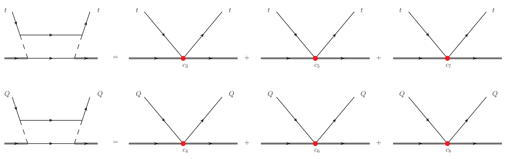
A.3 Quarks
We consider only couplings with top quarks, for while all other Yukawa couplings are negligible. In the fundamental theory, we compute the two matrix elements
| (69) | |||
| (70) |
describing respectively a scattering between a heavy Majorana neutrino at rest and a right-handed top quark carrying momentum , and a scattering between a heavy Majorana neutrino at rest and a left-handed heavy quark carrying momentum . The indices , , and are Lorentz indices, whereas and are the SU(2) indices of the heavy-quark doublet. The diagrams contributing to the matrix elements in the fundamental theory are shown in figure 6. We call the diagram with external top lines and the diagram with external heavy-quark lines. The imaginary parts of and read
| (71) | |||
| (72) |
where the dots stand for higher-order terms in the expansion or terms that are of order but do not depend on the momentum .
The matrix element (69) is matched in the EFT by
| (73) |
and the matrix element (70) by
| (74) |
where the dots in (73) and (74) stand for contributions coming from operators not listed in (23). Comparing (71) and (72) with the imaginary parts of (73) and (74) respectively, we obtain
| (75) | |||||
| (76) | |||||
| (77) |

A.4 Gauge bosons
The couplings of the Majorana neutrino with the gauge bosons are conveniently computed by considering in the fundamental theory the following two matrix elements
| (78) |
and
| (79) |
where and are indices labeling fields in the adjoint representation of SU(2), and and are spatial Lorentz indices. The matrix elements (78) and (79) describe scatterings between heavy Majorana neutrinos at rest and gauge bosons carrying momentum . Each diagram in the full theory, labeled according to figure 7, contributes with an imaginary part that reads for the (78) matrix element
| (80) | |||||
| (81) | |||||
| (82) | |||||
| (83) |
For the matrix element (79) the result is the same after the replacement . The dots stand for terms that are proportional to or or for terms of order or smaller.
The matrix element (78) is matched in the EFT by
| (84) |
and the matrix element (79) by
| (85) |
where the dots stand for contributions coming from operators not listed in (23). Summing up all contributions (80)-(83) for each of the two matrix elements and comparing with the imaginary parts of (84) and (85), we finally find
| (86) | |||||
| (87) |
The same Wilson coefficients satisfy the matching conditions for matrix elements with temporal gauge bosons.
References
- (1) M. Drewes, arXiv:1303.6912 [hep-ph].
- (2) Y. Fukuda et al. [Super-Kamiokande Collaboration], Phys. Rev. Lett. 81 (1998) 1562 [hep-ex/9807003].
- (3) S. N. Ahmed et al. [SNO Collaboration], Phys. Rev. Lett. 92 (2004) 181301 [nucl-ex/0309004].
- (4) P. Minkowski, Phys. Lett. B 67 (1977) 421.
- (5) M. Gell-Mann, P. Ramond and R. Slansky, Conf. Proc. C 790927 (1979) 315 [arXiv:1306.4669 [hep-th]].
- (6) R. N. Mohapatra and G. Senjanovic, Phys. Rev. Lett. 44 (1980) 912.
- (7) A. D. Dolgov, Phys. Rept. 222 (1992) 309.
- (8) E. Komatsu et al. [WMAP Collaboration], Astrophys. J. Suppl. 180 (2009) 330 [arXiv:0803.0547 [astro-ph]].
- (9) M. Fukugita and T. Yanagida, Phys. Lett. B 174 (1986) 45.
- (10) G. Bertone, D. Hooper and J. Silk, Phys. Rept. 405 (2005) 279 [hep-ph/0404175].
- (11) A. Boyarsky, O. Ruchayskiy and M. Shaposhnikov, Ann. Rev. Nucl. Part. Sci. 59 (2009) 191 [arXiv:0901.0011 [hep-ph]].
- (12) N. Isgur and M. B. Wise, Phys. Lett. B 232 (1989) 113.
- (13) E. Eichten and B. R. Hill, Phys. Lett. B 234 (1990) 511.
- (14) K. Kopp and T. Okui Phys. Rev. D 84 (2011) 093007 [arXiv:1108.2702 [hep-ph]].
- (15) A. Salvio, P. Lodone and A. Strumia, JHEP 1108 (2011) 116 [arXiv:1106.2814 [hep-ph]].
- (16) M. Laine and Y. Schröder, JHEP 1202 (2012) 068 [arXiv:1112.1205 [hep-ph]].
- (17) M. Neubert, Phys. Rept. 245 (1994) 259 [hep-ph/9306320].
- (18) M. J. Dugan, M. Golden and B. Grinstein, Phys. Lett. B 282 (1992) 142.
- (19) P. D. Mannheim, Int. J. Theor. Phys. 23 (1984) 643.
- (20) R. J. Hill and M. P. Solon, Phys. Lett. B 707 (2012) 539 [arXiv:1111.0016 [hep-ph]].
- (21) M. A. Luty, Phys. Rev. D 45 (1992) 455.
- (22) W. Buchmüller, R. D. Peccei and T. Yanagida, Ann. Rev. Nucl. Part. Sci. 55 (2005) 311 [hep-ph/0502169].
- (23) S. Davidson, E. Nardi and Y. Nir, Phys. Rept. 466 (2008) 105 [arXiv:0802.2962 [hep-ph]].
- (24) T. Asaka and M. Shaposhnikov, Phys. Lett. B 620 (2005) 17 [hep-ph/0505013].
- (25) T. Asaka, S. Blanchet and M. Shaposhnikov, Phys. Lett. B 631 (2005) 151 [hep-ph/0503065].
- (26) T. Asaka, M. Laine and M. Shaposhnikov, JHEP 0606 (2006) 053 [hep-ph/0605209].
- (27) N. Brambilla, D. Gromes and A. Vairo, Phys. Lett. B 576 (2003) 314 [arXiv:hep-ph/0306107].
- (28) M. Le Bellac, Thermal Field Theory, Cambridge University Press, Cambridge U.K. (1996).
- (29) N. Brambilla, J. Ghiglieri, A. Vairo and P. Petreczky, Phys. Rev. D 78 (2008) 014017 [arXiv:0804.0993 [hep-ph]].