shadows
The Long-Baseline Neutrino Experiment
Exploring Fundamental Symmetries of the Universe
April 15, 2014
Cover design by Diana Brandonisio, Fermilab Visual Media Services
Typeset in LaTeX
See pages - of lbne-sci-opp-auth.pdf
Contents
List of Figures
List of Tables
Abstract
The preponderance of matter over antimatter in the early Universe, the dynamics of the supernova bursts that produced the heavy elements necessary for life and whether protons eventually decay — these mysteries at the forefront of particle physics and astrophysics are key to understanding the early evolution of our Universe, its current state and its eventual fate. The Long-Baseline Neutrino Experiment (LBNE) represents an extensively developed plan for a world-class experiment dedicated to addressing these questions.
Experiments carried out over the past half century have revealed that neutrinos are found in three states, or flavors, and can transform from one flavor into another. These results indicate that each neutrino flavor state is a mixture of three different nonzero mass states, and to date offer the most compelling evidence for physics beyond the Standard Model. In a single experiment, LBNE will enable a broad exploration of the three-flavor model of neutrino physics with unprecedented detail. Chief among its potential discoveries is that of matter-antimatter asymmetries (through the mechanism of charge-parity violation) in neutrino flavor mixing — a step toward unraveling the mystery of matter generation in the early Universe. Independently, determination of the unknown neutrino mass ordering and precise measurement of neutrino mixing parameters by LBNE may reveal new fundamental symmetries of Nature.
Grand Unified Theories, which attempt to describe the unification of the known forces, predict rates for proton decay that cover a range directly accessible with the next generation of large underground detectors such as LBNE’s. The experiment’s sensitivity to key proton decay channels will offer unique opportunities for the ground-breaking discovery of this phenomenon.
Neutrinos emitted in the first few seconds of a core-collapse supernova carry with them the potential for great insight into the evolution of the Universe. LBNE’s capability to collect and analyze this high-statistics neutrino signal from a supernova within our galaxy would provide a rare opportunity to peer inside a newly-formed neutron star and potentially witness the birth of a black hole.
To achieve its goals, LBNE is conceived around three central components: (1) a new, high-intensity neutrino source generated from a megawatt-class proton accelerator at Fermi National Accelerator Laboratory, (2) a fine-grained near neutrino detector installed just downstream of the source, and (3) a massive liquid argon time-projection chamber deployed as a far detector deep underground at the Sanford Underground Research Facility. This facility, located at the site of the former Homestake Mine in Lead, South Dakota, is 1,300 km from the neutrino source at Fermilab — a distance (baseline) that delivers optimal sensitivity to neutrino charge-parity symmetry violation and mass ordering effects. This ambitious yet cost-effective design incorporates scalability and flexibility and can accommodate a variety of upgrades and contributions.
With its exceptional combination of experimental configuration, technical capabilities, and potential for transformative discoveries, LBNE promises to be a vital facility for the field of particle physics worldwide, providing physicists from institutions around the globe with opportunities to collaborate in a twenty to thirty year program of exciting science.
How to Read this Document
The LBNE science document is intended to inform a diverse readership about the goals and capabilities of the LBNE experiment. Your approach to reading this document will depend upon your purpose as well as your level of knowledge about high energy and neutrino physics.
![[Uncaptioned image]](1307.7335v3/figures/green_circle.png)
![[Uncaptioned image]](1307.7335v3/figures/blue_square.png)
The three chapters Chapter 1 Introduction and Executive Summary, Chapter 3 Project and Design and Chapter 9 Summary and Conclusion together provide a comprehensive overview of LBNE’s scientific objectives, its place in the landscape of neutrino physics experiments worldwide, the technologies it will incorporate and the capabilities it will possess. Much of the information in these chapters is accessible to the lay reader, but of course, the scientific concepts, goals and methods around which LBNE is designed are by their nature highly specialized, and the text in certain sections is correspondingly technical.
![[Uncaptioned image]](1307.7335v3/figures/black_diamond.png)
In Chapter 2 The Science of LBNE, the initial paragraphs in each section provide some introductory information, but in general this chapter assumes a working knowledge of high energy physics and, ideally, familiarity with neutrino physics.
The three chapters that delve into the areas corresponding to the scientific objectives of LBNE: Chapter 4 Neutrino Mixing, Mass Hierarchy and CP Violation, Chapter 5 Nucleon Decay Motivated by Grand Unified Theories and Chapter 6 Core-Collapse Supernova Neutrinos, assume a working knowledge of high energy physics and particle astrophysics. This is also true of Chapter 7 Precision Measurements with a High-Intensity Neutrino Beam and Chapter 8 Additional Far Detector Physics Opportunities, as well as the appendices.
Introduction and
Executive Summary
1.1 Overview
Although neutrinos are the most abundant of known matter particles (fermions) in the Universe, their properties are the least well understood. The very existence of neutrino mass constitutes evidence of physics beyond the Standard Model. Understanding the nature of neutrinos has consequently become an essential goal for particle physics.
Observations of oscillations of neutrinos from one type (flavor) to another in numerous recent experiments have provided evidence for neutrino flavor mixing and for small, but nonzero, neutrino masses. The framework characterizing these observations is similar to that describing corresponding phenomena in the quark sector, but with a very different pattern of mixing angle values. As in the quark case, this framework involves a phase parameter, , that changes sign under combined charge conjugation and parity (CP) reversal operations and thus would lead to CP symmetry-violating asymmetries between the pattern of oscillations for neutrinos and antineutrinos. While groundbreaking on its own, the observation of such asymmetries would also provide an experimental underpinning for the basic idea of leptogenesis11 1 Leptogenesis refers to the mechanisms that generated an asymmetry between leptons and antileptons in the early Universe, described in Section 2.2.1. as an explanation for the Baryon Asymmetry of the Universe (BAU).
Neutrino oscillation data so far tell us about differences in the squared masses of the neutrino mass states, and about the sign of the mass-squared difference between two of the states, but not about the difference of those with respect to the third, which may be heavier (normal ordering) or lighter (inverted ordering) than the other two. Resolving this neutrino mass hierarchy ambiguity, along with precise measurements of neutrino mixing angles, would have significant theoretical, cosmological and experimental implications. One important consequence of mass hierarchy determination, in particular, would be the impact on future experiments designed to determine whether — uniquely among the fundamental fermions — neutrinos are their own antiparticles, so-called Majorana particles. Though long suspected, this hypothesis that neutrinos are Majorana particles has yet to be either established or ruled out. Strong evidence for the inverted hierarchy would establish conditions required by the next generation of neutrinoless double-beta decay searches to settle this question even with a null result (no observation). Because the forward scattering of neutrinos in matter alters the oscillation pattern in a hierarchy-dependent way, the long baseline of LBNE — with the neutrinos traveling through the Earth’s mantle — enables a decisive determination of the hierarchy, independent of the value of .
Additionally, the high-precision determination of oscillation parameters such as mixing angles and squared-mass differences will provide insight into the differences between the quark and lepton mixing patterns, which is necessary for deciphering the flavor structure of physics in the Standard Model. Taken together, the above suite of measurements will thoroughly test the standard three-neutrino flavor paradigm that guides our current understanding, and will provide greatly extended sensitivity to signatures for nonstandard neutrino interactions in matter.
The arena of non-accelerator physics using massive underground detectors such as the LBNE far detector is also ripe with discovery potential. The observation of nucleon decay would be a watershed event for the understanding of physics at high energy scales. Neutrinos from supernovae are expected to provide key insights into the physics of gravitational collapse, and may also reveal fundamental properties of the neutrino.
Among massive detectors designed for neutrino and nucleon decay physics, the LArTPC technology offers unmatched capabilities for position and energy resolution and for high-precision reconstruction of complex interaction topologies over a broad energy range. It also provides a compact, scalable approach for achieving the required sensitivity to the primary physics signatures to be explored by LBNE. As these capabilities are also important for non-accelerator neutrino physics, LBNE will complement the large, underground water Cherenkov and/or scintillator-based detectors that may be operating in parallel. LArTPC detectors are especially well-suited to proton decay modes such as the supersymmetry-favored mode, uniquely providing detection efficiency and background rejection sufficient to enable a discovery with a single well-reconstructed event. With regard to supernova-neutrino detection, liquid argon detectors are primarily sensitive to the component of the flux, while interactions dominate for water and scintillator-based detectors. Thus, LBNE will be sensitive to different features of the supernova-neutrino production process. Finally, the LArTPC technology opens up an avenue for precision studies of oscillation physics with atmospheric neutrinos, thereby augmenting the results of the beam-based measurements at the core of the experiment.
The highly capable near detector will measure the absolute flux and energy scales of all four neutrino species in the LBNE beam, as well as neutrino cross sections on argon, water, and other nuclear targets in the beam’s energy range. These measurements are needed to attain the ultimately desired precision of the oscillation parameter measurements. Additionally, the near detector will enable a broad range of precision neutrino-interaction measurements, thereby adding a compelling scientific program of its own.
The unique combination in LBNE of a baseline, exceptional resolution, large target mass and deep underground location offers opportunity for discovery of entirely unanticipated phenomena. History shows that ambitious scientific endeavors with leading-edge instruments have often been rewarded with unexpected signatures of new physics.
LBNE is an extensively developed experiment whose execution will have substantial impact on the overall direction of high energy physics (HEP) in the U.S. The U.S. Department of Energy (DOE) has endorsed the science objectives of LBNE, envisioning the experiment as a phased program, and has given first stage (CD-1) approval with a budget of $867M toward the initial phase. The science scope of this and subsequent phases will depend on the level of investment by additional national and international partners.
This document outlines the LBNE physics program and how it may evolve in the context of long-term planning studies [1]. The physics reach of this program is summarized under scenarios that are consistent with short-, medium- and long-term considerations. The general conclusions regarding the scientific capabilities of LBNE in a phased program are twofold:
- 1.
A full-scope LBNE will provide an exciting broad-based physics program with exceptional capabilities for all of the identified core physics objectives, and many additional ones.
- 2.
A first phase with a LArTPC far detector of fiducial22 2 In neutrino experiments, not all neutrino interactions in the instrumented (active) volume of a detector are used for physics studies. Only interactions that are well contained within the instrumented volume are used. The smaller volume of detector that encompasses the neutrino interactions is known as the fiducial volume and the target mass contained within it is known as the fiducial mass. Unless otherwise noted, this document will use fiducial mass to characterize the far detector size. mass 33 3 The kt refers to a metric kiloton, equivalent to . or greater will substantially advance the field of neutrino oscillation physics while laying the foundations for a broader physics program in a later phase.
1.2 Development of a World-Class Experiment
The concept of a high-intensity neutrino beam directed toward a distant, massive underground detector to simultaneously investigate the nature of the neutrino, proton decay and astrophysical sources of neutrinos has been under serious investigation since the late 1990s [2, 3, 4, 5, 6, 7, 8, 9]. Since that time both the science goals and concepts for implementation have been the subject of intense study and review by distinguished panels. These panels include the National Academies Neutrino Facilities Assessment Committee in 2003 [10], the National Science and Technology Council Committee on Science in 2004 [11], the National Academies EPP2010 panel in 2006 [12], the HEPAP/NSAC Neutrino Scientific Assessment Group in 2007 [13], the HEPAP Particle Physics Project Prioritization Panel (P5) in 2008 [14], the National Academies ad hoc Committee to Assess the Science Proposed for DUSEL in 2011 [15], and most recently the HEPAP Facilities Subpanel in 2013 [16]. High-level studies performed in Europe and Asia have come to similar conclusions (e.g., [17]) about the merits and feasibility of such a program.
1.2.1 Long-Term Vision
LBNE as described in this document has been developed by a collaboration formally established in 2009, which currently comprises over 475 collaborators from over 80 institutions in six countries. In January 2010 the DOE formally recognized the LBNE science objectives with approval of the mission need statement (CD-0) [18]. This action established LBNE as a DOE project. Fermilab has recognized LBNE as a central component of its long-term future program.
The central role of LBNE within the U.S. particle physics program has been acknowledged in other documents prepared for the 2013 particle physics community planning exercise [1], including the Project X Physics Book [19] and the reports from Intensity Frontier working groups on neutrino physics [20] and baryon number violation [21].
The LBNE conceptual design reflects a flexible and cost-effective approach to next-generation neutrino physics experiments that maintains a world-leadership role for the U.S. over the long term. The full-scope LBNE includes a fiducial mass ( total) far detector located in a new experimental area to be excavated at the 4,850-ft level of the Sanford Underground Research Facility 44 4 Much larger detectors could also be accommodated at this facility. in the former Homestake Mine, and a fine-grained near neutrino detector located on the Fermilab site. Simultaneous construction of a new neutrino beamline at Fermilab would permit operation with an initial beam power of , enabled by upgrades to the front end of the accelerator complex carried out within the Proton Improvement Plan-II (PIP-II) program [22]. In anticipation of potential enhancements beyond PIP-II [23], the beamline is designed to support upgrades to accommodate a beam power of . The baseline is in the optimal range for the neutrino oscillation program. The cosmic ray shielding provided by the deep underground site for the far detector enables the non-accelerator portion of the physics program, including proton decay searches, detailed studies of neutrino bursts from galactic supernovae, and precision analyses of atmospheric-neutrino samples.
The overall physics reach of LBNE is predominantly limited by detector mass. From the outset, a guiding principle of the far detector design has been scalability. The conceptual design for the full-scope detector, consisting of two identical ( total) TPC modules housed within separate vessels (cryostats), employs technology developed by the liquefied natural gas (LNG) storage and transport industry. The TPC modules themselves consist of arrays of modular anode and cathode plane assemblies (APAs and CPAs) that are suspended from rails affixed to the top of the cryostats. The APA/CPA dimensions are chosen for ease of transportation and installation. The modularity of the detectors allows flexibility in the geometry and phased construction of the LBNE far detector complex. Cost-effective designs for larger detector masses are readily obtained by increasing the vessel size and simply adding APA/CPA units, thereby also exploiting economies of scale and benefiting from an increased ratio of volume to surface area. Detector mass may also be increased through the addition of distinct detectors of the same or a different technology, either during initial construction or in a later phase.
1.2.2 Present Status of the LBNE Project
Since DOE CD-0 approval, a compete conceptual design for the full-scope LBNE has been developed, consisting of a LArTPC far detector located feet underground, a baseline, a highly capable near neutrino detector, and a multi-megawatt-capable neutrino beamline. This design has been thoroughly reviewed, and found to be sound, most recently at a Fermilab Director’s CD-1 Readiness Review in March 2012 [24]. Since then, considerable effort has been devoted to understanding how the LBNE Project can be staged so as to accommodate anticipated budget conditions while maintaining compelling physics output at each stage [25]. This process led to a first-phase configuration that was reviewed by the DOE in October [26] and November 2012 [27], and that received CD-1 approval [28] in December 2012. This configuration [29, 30, 31, 32, 33, 34] maintained the most important aspects of LBNE: the baseline to the Sanford Underground Research Facility, a large — of order tens of kilotons in fiducial mass — LArTPC far detector design, and a multi-megawatt-capable, wide-band neutrino/antineutrino beam. However, the far detector size was limited at CD-1 to and placed at the surface under minimal overburden, and the near detector was deferred to a later phase.
The DOE CD-1 approval document [28] explicitly allows adjustment of the scope of the first phase of LBNE in advance of CD-2 if additional partners bring significant contributions to LBNE. Using the CD-1 DOE funding as the foundation, the goal for the first phase of LBNE is a deep underground far detector of at least , placed in a cavern that will accommodate up to a detector, coupled with a neutrino beamline, and a highly capable near detector. This goal has been endorsed by the LBNE Collaboration, the LBNE Project, the Fermilab directorate, and the DOE Office of High Energy Physics. Since a large portion of the LBNE Project cost is in civil infrastructure, funding contributions from new partners could have considerable impact on the experimental facilities, and therefore the physics scope, in the first phase.
1.2.3 Global Partnerships
Global conditions are favorable for significant international partnerships in developing and building LBNE. As an example, the 2013 update [17] of the European Strategy for Particle Physics document places long-baseline neutrino physics among the highest-priority large-scale activities for Europe, recognizing that it requires “significant resources, sizeable collaborations and sustained commitment.” It includes the primary recommendation of exploring “the possibility of major participation in leading long-baseline neutrino projects in the U.S. and Japan.” As of March 2014 the LBNE Collaboration includes institutions from the U.S., Brazil, India, Italy, Japan and the United Kingdom. Discussions with a number of potential international partners are underway — some already at an advanced stage. A summary of recent progress in these discussions can be found in the presentation of LBNE status to the U.S. Particle Physics Projects Prioritization Panel in November 2013 [35].
1.2.4 Context for Discussion of Physics Sensitivities
To reflect the physics reach of various phasing scenarios, this document presents many of the parameter sensitivities for the accelerator-based neutrino topics as functions of exposure, defined as the product of detector fiducial mass, beam power and run time. As needed, the capabilities of both a first-phase configuration and the full configuration are explicitly highlighted, each benchmarked for six to ten years of operations with a beam power from the PIP-II accelerator upgrades at Fermilab. Since the U.S. program planning exercises currently under way look beyond the present decade, this document also presents the long-term physics impact of the full-scope LBNE operating with the beam power available with further anticipated upgrades to the Fermilab accelerator complex.
1.3 The LBNE Physics Program
This section summarizes LBNE’s potential for achieving its core physics objectives based on the current experimental landscape, scenarios for staging LBNE, and the technical capabilities of LBNE at each stage.
LBNE’s capability to achieve the physics objectives described in this document has been subject to extensive review over a number of years. In addition to the various reviews of the LBNE Project described in Section 1.2, reviews that focused strongly on LBNE’s science program include the DOE Office of Science Independent Review of Options for Underground Science in the spring of 2011 [36], the LBNE Science Capabilities Review (by an external panel commissioned by LBNE) [37] in the fall of 2011, and the LBNE Reconfiguration Review [25] in the summer of 2012.
1.3.1 Neutrino Mixing, Mass Hierarchy and CP Violation
Neutrino Mass Hierarchy: The baseline establishes one of LBNE’s key strengths: sensitivity to the matter effect. This effect leads to a large discrete asymmetry in the versus oscillation probabilities, the sign of which depends on the mass hierarchy (MH). At this asymmetry is approximately in the region of the peak flux; this is larger than the maximal possible CP-violating asymmetry associated with , meaning that both the MH and can be determined unambiguously with high confidence within the same experiment using the beam neutrinos.
In detail, the sensitivity of LBNE depends on the actual values of poorly known mixing parameters (mainly and ), as well as the true value of the MH itself. The discrimination between the two MH hypotheses is characterized as a function of the a priori unknown true value of by considering the difference, denoted , between the values calculated for a data set with respect to these hypotheses, considering all possible values of 55 5 For the case of the MH determination, the usual association of this test statistic with a distribution for one degree of freedom is incorrect; additionally the assumption of a Gaussian probability density implicit in this notation is not exact. The discussion in Chapter 4 provides a brief description of the statistical considerations.. In terms of this test statistic, the MH sensitivity of LBNE with , and running three years each in and modes in a beam is illustrated in Figure 1.1 for the case of normal hierarchy for two different values of .
Across the overwhelming majority of the parameter space for the mixing parameters that are not well known (mainly and ), LBNE’s determination of the MH will be definitive, but even for unfavorable combinations of the parameter values, a statistically ambiguous outcome is highly unlikely.
The least favorable scenario corresponds to a true value of in which the MH asymmetry is maximally offset by the leptonic CP asymmetry, and where, independently, takes on a value at the low end of its experimentally allowed range. For this scenario, studies indicate that with a LArTPC operating for six years in a beam, LBNE on its own can (in a typical data set) distinguish between normal and inverted hierarchy with . This corresponds to a probability of determining the correct hierarchy. In of data sets, LBNE will measure in this scenario, where measuring with an expected value of corresponds to a significance in excess of three Gaussian standard deviations.
Concurrent analysis of the corresponding atmospheric-neutrino samples in an underground detector will improve the precision with which the MH is resolved. It is important to note that for the initial stages of LBNE, a greatly improved level of precision in the determination of the MH can be achieved by incorporating constraints from NOA and T2K data. With an initial detector, for half the range of possible values, the expected significance exceeds ; again this corresponds to a probability of determining the correct hierarchy. To put this in context, it is notable that even an extended NOA program [38] at four times its nominal exposure (of six years of operation at ), would have coverage at the level or better for only of the range.
CP Violation and the Measurement of : The LBNE program has two somewhat distinct objectives with regard to CP symmetry violation in the oscillation channel. First, LBNE aims to make a precise determination of the value of within the context of the standard three-flavor mixing scenario described by the PMNS matrix (discussed in Section 2.2). Second, and perhaps more significantly, LBNE aims to observe a signal for leptonic CP violation, independent of the underlying nature of neutrino oscillation phenomenology. Within the standard three-flavor mixing scenario, such a signal will be observable, provided is not too close to either of the values for which there is no CP violation (zero and ). Together, the pursuit of these two goals provides a thorough test of the standard three-flavor scenario.
Figure 1.2 shows the expected 1 resolution for as a function of exposure for a proton beam power of . At this beam power, in a six-year run, a far detector will be able to measure to 20∘ 30∘ (depending on its value), independent of other experiments. A full-scope LBNE operating with multi-megawatt beam power in a later phase, will achieve a precision better than , comparable to the current precision on the CP phase in the CKM matrix in the quark sector.
LBNE with a detector, in combination with T2K and NOA, will determine leptonic CP violation with a precision of or greater for of values in a six-year run with beam power. It is important to note that LBNE alone dominates the combined sensitivity and that T2K and NOA have very limited sensitivity to CP violation on their own. To reach for an appreciable fraction of the range of , the full-scope LBNE will be needed to control systematic errors while accumulating large enough samples in the far detector to reach this level of sensitivity. No experiment can provide coverage at 100%, since CP violation effects vanish as or .
Determination of and Octant Resolution: In long-baseline experiments with beams, the magnitude of disappearance and appearance signals is proportional to and , respectively, in the standard three-flavor mixing scenario. Current disappearance data are consistent with maximal mixing, . To obtain the best sensitivity to both the magnitude of its deviation from as well as its sign ( octant), a combined analysis of the two channels is needed [39]. As demonstrated in Chapter 4, a LBNE detector will be able to resolve the octant at the level or better for values less than or greater than , provided is not too close to zero or . A full-scope LBNE will measure with a precision of or less, even for values within a few degrees of .
1.3.2 Nucleon Decay Physics Motivated by Grand Unified Theories
The LBNE far detector will significantly extend lifetime sensitivity for specific nucleon decay modes by virtue of its high detection efficiency relative to water Cherenkov detectors and its low background rates. As an example, LBNE has enhanced capability for detecting the channel, where lifetime predictions from supersymmetric models extend beyond, but remain close to, the current (preliminary) Super-Kamiokande limit of (90% CL) from a exposure [40]66 6 The lifetime shown here is divided by the branching fraction for this decay mode, , and as such is a partial lifetime.. The signature for an isolated semi-monochromatic charged kaon in a LArTPC is distinctive, with multiple levels of redundancy. A LBNE far detector deep underground will reach a limit of after ten years of operation (Figure 1.3), and would see nine events with a background of 0.3 should be , just beyond the current limit. Even a detector (placed underground) would yield an intriguing signal of a few events after a ten-year exposure in this scenario.

1.3.3 Supernova-Neutrino Physics and Astrophysics
The neutrinos from a core-collapse supernova are emitted in a burst of a few tens of seconds duration, with about half in the first second. Energies are in the range of a few tens of MeV, and the luminosity is divided roughly equally between the three known neutrino flavors. Currently, experiments worldwide are sensitive primarily to electron antineutrinos (), with detection through the inverse-beta decay process on free protons77 7 This refers to neutrino interactions with the nucleus of a hydrogen atom in H2O in water detectors or in hydrocarbon chains in liquid scintillator detectors., which dominates the interaction rate in water and liquid-scintillator detectors. Liquid argon has a unique sensitivity to the electron-neutrino () component of the flux, via the absorption interaction on 40Ar as follows:
This interaction can be tagged via the coincidence of the emitted electron and the accompanying photon cascade from the de-excitation. About 900 events would be expected in a fiducial mass liquid argon detector for a supernova at a distance of . In the neutrino channel the oscillation features are in general more pronounced, since the spectrum is always significantly different from the () spectra in the initial core-collapse stages, to a larger degree than is the case for the corresponding spectrum. Detection of a large neutrino signal in LBNE would help provide critical information on key astrophysical phenomena such as
- 1.
the neutronization burst
- 2.
formation of a black hole
- 3.
shock wave effects
- 4.
shock instability oscillations
- 5.
turbulence effects
1.3.4 Precision Measurements with a High-Intensity Neutrino Source and High-Resolution Near Detector
The near neutrino detector will provide precision measurements of neutrino interactions, which in the medium to long term are essential for controlling the systematic uncertainties in the long-baseline oscillation physics program. The near detector, which will include argon targets, will measure the absolute flux and energy-dependent shape of all four neutrino species, , , and to accurately predict for each species the far/near flux ratio as a function of energy. It will also measure the four-momenta of secondary hadrons, such as charged and neutral mesons, produced in the neutral and charged current interactions that constitute the dominant backgrounds to the oscillation signals.
With () () charged current and () neutral current interactions per ton per protons-on-target at in the () beam, the near detector will also be the source of data for a rich program of neutrino-interaction physics in its own right. These numbers correspond to neutrino interactions per year for the range of beam configurations and near detector designs under consideration. Measurement of fluxes, cross sections and particle production over a large energy range of (which can also help constrain backgrounds to proton decay signals from atmospheric neutrinos) are the key elements of this program. Furthermore, since the near detector data will feature very large samples of events that are amenable to precision reconstruction and analysis, they can be exploited for sensitive studies of electroweak physics and nucleon structure, as well as for searches for new physics in unexplored regions (heavy sterile neutrinos, high- oscillations, light Dark Matter particles, and so on).
1.4 Summary
This chapter has touched only briefly on the most prominent portion of the full suite of physics opportunities enabled by LBNE. The following chapters cover these in detail, as well as topics that were omitted here in the interest of brevity and focus. In Chapter 9 progress toward LBNE physics milestones is addressed, based on one potential scenario for the operation of successive stages of LBNE detector and PIP-II implementations, and the broad role of LBNE is discussed in the context of such scenarios. The present chapter concludes with a summary of its key points.
The primary science goals of LBNE are drivers for the advancement of particle physics. The questions being addressed are of wide-ranging consequence: the origin of flavor and the generation structure of the fermions (i.e., the existence of three families of quark and lepton flavors), the physical mechanism that provides the CP violation needed to generate the Baryon Asymmetry of the Universe, and the high energy physics that would lead to the instability of matter. Achieving these goals requires a dedicated, ambitious and long-term program. No other proposed long-baseline neutrino oscillation program with the scientific scope and sensitivity of LBNE is as advanced in terms of engineering development and project planning. A phased program with a far detector of even modest size in the initial stage (e.g., 10 kt) will enable exciting physics in the intermediate term, including a definitive mass hierarchy determination and a measurement of the CP phase without ambiguities, while providing the fastest route toward achieving the full range of LBNE’s science objectives. Should LBNE find that the CP phase is not zero or , it will have found strong indications () of leptonic CP violation. Global interest is favorable for contributions from international partners to accelerate and enhance this program, including the LBNE first-phase scope.
Implementing the vision that has brought LBNE to this point will allow the U.S. to host this world-leading program, bringing together the world’s neutrino community to explore key questions at the forefront of particle physics and astrophysics. Moreover, the excitement generated by both the technical challenges of mounting LBNE and the potential physics payoffs are widely shared — among the generation of scientists who have been paving the way for these innovations, as well as the young scientists for whom LBNE will provide numerous research opportunities over the next two decades.
The Science
of LBNE
LBNE has been designed to address a wide range of scientific topics using well-characterized, high-intensity, accelerator-based neutrino beams, a long baseline for neutrino oscillations, and a very large, deep-underground detector with excellent particle identification capabilities over a large range of energies. While maximizing the reach for a core set of scientific objectives, its design — described in Chapter 3 — accommodates the flexibility to extend the scope of measurements as additional resources become available.
2.1 Scientific Objectives of LBNE
The scientific objectives of LBNE have been categorized into primary, secondary, and additional secondary objectives according to priorities developed and agreed upon by the LBNE community and accepted as part of the CD-0 (Mission Need) approval by the U.S. Department of Energy [41].
Primary objectives of LBNE, in priority order, are the following measurements:
- 1.
precision measurements of the parameters that govern oscillations; this includes precision measurement of the third mixing angle , measurement of the charge-parity (CP) violating phase , and determination of the neutrino mass ordering (the sign of ), the so-called mass hierarchy
- 2.
precision measurements of the mixing angle , including the determination of the octant in which this angle lies, and the value of the mass difference, ||, in oscillations
- 3.
search for proton decay, yielding significant improvement in the current limits on the partial lifetime of the proton (/BR) in one or more important candidate decay modes, e.g.,
- 4.
detection and measurement of the neutrino flux from a core-collapse supernova within our galaxy, should one occur during the lifetime of LBNE
In a phased approach to LBNE, the goal of the first phase is to maximize the effectiveness of the facility to achieve the first two objectives, above. The mass hierarchy determination and the precision determination of will most likely be complete in the first phase of LBNE; while the precision determination of CP violation will require the full-scope LBNE, an initial measurement of the CP phase parameter will be performed in earlier phases.
Secondary objectives, which may also be enabled by the facility designed to achieve the primary objectives, include:
- 1.
other accelerator-based, neutrino oscillation measurements; these could include further sensitivity to Beyond Standard Model (BSM) physics such as nonstandard interactions
- 2.
measurements of neutrino oscillation phenomena using atmospheric neutrinos
- 3.
measurement of other astrophysical phenomena using medium-energy neutrinos
Additional secondary objectives, the achievement of which may require upgrades to the facility that is designed to achieve the primary physics objectives (e.g., deployment of additional detector mass or alternate detector technologies), include:
- 1.
detection and measurement of the diffuse supernova-neutrino flux
- 2.
measurements of neutrino oscillation phenomena and of solar physics using solar neutrinos
- 3.
measurements of astrophysical and geophysical neutrinos of low energy
In addition, a rich set of science objectives enabled by a sophisticated near neutrino detector have been identified. A primary and a secondary objective, respectively, are:
- 1.
measurements necessary to achieve the primary physics research objectives listed above
- 2.
studies of neutrino interactions that may be enabled either by the facility designed to achieve the primary objectives or by future upgrades to the facility and detectors; these include precision studies of the weak interaction, studies of nuclear and nucleon structure, and searches for new physics
2.2 Neutrino Three-Flavor Mixing, CP Violation and the Mass Hierarchy
The Standard Model of particle physics (Figure 2.1) presents a remarkably accurate description of the elementary particles and their interactions. However, its limitations beg deeper questions about Nature. The unexplained patterns of quarks, leptons, flavors and generations imply that a more fundamental underlying theory must exist. LBNE plans to pursue a detailed study of neutrino mixing, resolve the neutrino mass ordering, and search for CP violation in the lepton sector by studying the oscillation patterns of high-intensity and beams measured over a long baseline.
Neutrino oscillation arises from mixing between the flavor and mass eigenstates of neutrinos, corresponding to the weak and gravitational interactions, respectively. This three-flavor-mixing scenario can be described by a rotation between the weak-interaction eigenstate basis and the basis of states of definite mass . In direct correspondence with mixing in the quark sector, the transformations between basis states is expressed in the form of a complex unitary matrix, known as the PMNS matrix :
| (2.1) |
The PMNS matrix in full generality depends on just three mixing angles and a CP-violating phase. The mixing angles and phase are designated as and . This matrix can be parameterized as the product of three two-flavor mixing matrices as follows, where and :
| (2.2) |
The parameters of the PMNS matrix determine the probability amplitudes of the neutrino oscillation phenomena that arise from mixing.
The relationship between the three mixing angles , and and the mixing between the neutrino flavor and mass states can be described as follows [45]: (2.3) (2.4) (2.5) The frequency of neutrino oscillation among the weak-interaction (flavor) eigenstates depends on the difference in the squares of the neutrino masses, ; a set of three neutrino mass states implies two independent mass-squared differences ( and ). The ordering of the mass states is known as the neutrino mass hierarchy. An ordering of is known as the normal hierarchy since it matches the ordering of the quarks in the Standard Model, whereas an ordering of is referred to as the inverted hierarchy. Since each flavor eigenstate is a mixture of three mass eigenstates, there can be an overall phase difference between the quantum states, referred to as . A nonzero value of this phase implies that neutrinos and antineutrinos oscillate differently — a phenomenon known as charge-parity (CP) violation. is therefore often referred to as the CP phase or the CP-violating phase.The entire complement of neutrino experiments to date has measured five of the mixing parameters: the three angles , and (recently) , and the two mass differences and . The sign of is known, but not that of , which is the crux of the mass hierarchy ambiguity. The values of and are large, while is smaller [46]. The value of is unknown. The real values of the entries of the PMNS mixing matrix, which contains information on the strength of flavor-changing weak decays in the lepton sector, can be expressed in approximate form as
| (2.6) |
The three-flavor-mixing scenario for neutrinos is now well established. However, the mixing parameters are not known to the same precision as are those in the corresponding quark sector, and several important quantities, including the value of and the sign of the large mass splitting, are still undetermined. In addition, several recent anomalous experimental results count among their possible interpretations phenomena that do not fit this model [47, 48, 49, 50].
The relationships between the values of the parameters in the neutrino and quark sectors suggest that mixing in the two sectors is qualitatively different. Illustrating this difference, the value of the entries of the CKM quark-mixing matrix (analogous to the PMNS matrix for neutrinos, and thus indicative of the strength of flavor-changing weak decays in the quark sector) can be expressed in approximate form as
| (2.7) |
and compared to the entries of the PMNS matrix given in Equation 2.6. As discussed in [51], the question of why the quark mixing angles are smaller than the lepton mixing angles is an important part of the “flavor problem.”
Quoting the discussion in [20], “while the CKM matrix is almost proportional to the identity matrix plus hierarchically ordered off-diagonal elements, the PMNS matrix is far from diagonal and, with the possible exception of the element, all elements are .” One theoretical method often used to address this question involves the use of non-Abelian discrete subgroups of as flavor symmetries; the popularity of this method comes partially from the fact that these symmetries can give rise to the nearly tri-bi-maximal11 1 Tri-bi-maximal mixing refers to a form of the neutrino mixing matrix with effective bimaximal mixing of and at the atmospheric scale ( ) and effective trimaximal mixing for with and at the solar scale ( ) [52]. structure of the PMNS matrix. Whether employing these flavor symmetries or other methods, any theoretical principle that attempts to describe the fundamental symmetries implied by the observed organization of quark and neutrino mixing — such as those proposed in unification models — leads to testable predictions such as sum rules between CKM and PMNS parameters [20, 42, 51, 53]. Data on the patterns of neutrino mixing are already proving crucial in the quest for a relationship between quarks and leptons and their seemingly arbitrary generation structure. Table 2.1 displays the comparison between quark and lepton mixing in terms of the fundamental parameters and the precision to which they are known22 2 A global fit [54] to existing results from current experiments sensitive to neutrino oscillation effects is the source for the PMNS matrix values., highlighting the limited precision of the neutrino-mixing parameter measurements.
| Parameter | Value (neutrino PMNS matrix) | Value (quark CKM matrix) |
|---|---|---|
| eV2 | ||
| eV2 | ||
Clearly much work remains in order to complete the standard three-flavor mixing picture, particularly with regard to (is it less than, greater than, or equal to ?), mass hierarchy (normal or inverted?) and . Additionally, there is great value in obtaining a set of measurements for multiple parameters from a single experiment, so that correlations and systematic uncertainties can be handled properly. Such an experiment would also be well positioned to extensively test the standard picture of three-flavor mixing. LBNE is designed to be this experiment.
2.2.1 CP Violation in the Quark and Lepton Sectors
In the particular parameterization of the PMNS matrix shown in Equation 2.2, the middle factor, labeled ‘II’, describes the mixing between the and mass states, and depends on the CP-violating phase . In the three-flavor model, leptonic CP violation in an oscillation mode occurs due to the interference of contributions from terms in this factor — some of which contain (i.e., involve the - mixing directly) and some of which do not. The presence of nonzero CP-odd terms, e.g., Equation 2.15, (which requires or ) in the interference patterns would result in an asymmetry in neutrino versus antineutrino oscillations. The magnitude of the CP-violating terms in the oscillation depends most directly on the size of the Jarlskog Invariant [56], a function that was introduced to provide a measure of CP violation independent of mixing-matrix parameterization. In terms of the three mixing angles and the (as yet unmeasured) CP-violating phase, the Jarlskog Invariant is:
| (2.8) |
The relatively large values of the mixing angles in the lepton sector imply that leptonic CP-violation effects may be quite large — depending on the value of the phase , which is currently unknown. Experimentally, it is unconstrained at the 2 level by the global fit [54]. Many theoretical models, examples of which include [57, 58, 59, 60, 61, 62], provide predictions for , but these predictions range over all possible values so do not yet provide any guidance.
Given the current best-fit values of the mixing angles [54] and assuming normal hierarchy,
| (2.9) |
This is in sharp contrast to the very small mixing in the quark sector, which leads to a very small value of the corresponding quark-sector Jarlskog Invariant [55],
| (2.10) |
despite the large value of .
To date, all observed CP-violating effects have occurred in experiments involving systems of quarks, in particular strange and -mesons [55]. Furthermore, in spite of several decades of experimental searches for other sources of CP violation, all of these effects are explained by the CKM quark-mixing paradigm, and all are functions of the quark-sector CP phase parameter, . In cosmology, successful synthesis of the light elements after the Big Bang [63, 64] (Big Bang Nucleosynthesis) requires that there be an imbalance in the number of baryons and antibaryons to one part in a billion when the Universe is a few minutes old [65]. CP violation in the quark sector has not, however, been able to explain the observed Baryon Asymmetry of the Universe (BAU), due to the small value of .
Baryogenesis [66] is a likely mechanism for generating the observed matter-antimatter asymmetry of our Universe. One way that it is elegantly achieved is by first having leptogenesis in the very early Universe. That mechanism can come about from the production and decay of very heavy right-handed neutrinos, if they are Majorana states (i.e. do not conserve lepton number33 3 In the Standard Model, lepton number () and baryon number () are conserved quantum numbers. Leptons have and and antileptons have . A quark has and and an antiquark has . ), CP symmetry is violated in their decays (thus distinguishing particles and antiparticles) and the Universe is in non-equilibrium. Leptogenesis will lead to an early dominance of antileptons over leptons. When the cooling Universe reaches the electroweak phase transition, , a baryon number excess is generated from the lepton asymmetry by a conserving mechanism (analogous to proton decay in that it violates and separately but conserves ) already present in the Standard Model.
The heavy Majorana right-handed neutrino states that could give rise to leptogenesis in the very early Universe are also a natural consequence of the GUT-based seesaw mechanism [67] — the simplest and most natural explanation of the observed super-light neutrino mass scales. The seesaw mechanism is a theoretical attempt to reconcile the very small masses of neutrinos to the much larger masses of the other elementary particles in the Standard Model. The seesaw mechanism achieves this unification by assuming an unknown new physics scale that connects the observed low-energy neutrino masses with a higher mass scale that involves very heavy sterile neutrino states. The seesaw mechanism as generator of neutrino mass is in addition to the Higgs mechanism that is now known to be responsible for the generation of the quark, charged lepton, and vector boson masses.
The no-equilibrium leptogenesis ingredient is expected in a hot Big Bang scenario, but the Majorana nature of the heavy neutrinos and needed CP violation can only be indirectly inferred from light neutrino experiments by finding lepton number violation (validating their Majorana nature via neutrinoless double-beta decay) and observing CP violation in ordinary neutrino oscillations.
Recent theoretical advances have demonstrated that CP violation, necessary for the generation of the Baryon Asymmetry of the Universe at the GUT scale (baryogenesis), can be directly related to the low-energy CP violation in the lepton sector that could manifest in neutrino oscillations. As an example, the theoretical model described in [68] predicts that leptogenesis, the generation of the analogous lepton asymmetry, can be achieved if (2.11) This implies given the latest global fit value of [69].The goal of establishing an experimental basis for assessing this possibility should rank very high on the list of programmatic priorities within particle physics, and can be effectively addressed by LBNE.
2.2.2 Observation of CP-Violating Effects in Neutrino Oscillation Experiments
Whereas the Standard Model allows for violation of charge-parity (CP) symmetries in weak interactions, CP transformations followed by time-reversal transformations (CPT) are invariant. Under CPT invariance, the probabilities of neutrino oscillation and antineutrino oscillation are equivalent, i.e., where . Measurements of oscillations in which the flavor of the neutrino before and after oscillations remains the same are referred to as disappearance or survival measurements. CPT invariance in neutrino oscillations was recently tested by measurements of and oscillations [70]; no evidence for CPT violation was found. Therefore, asymmetries in neutrino versus antineutrino oscillations arising from CP violation effects can only be accessed in appearance experiments, defined as oscillations of , in which the flavor of the neutrino after oscillations has changed. Because of the intrinsic challenges of producing and detecting ’s, the oscillation modes provide the most promising experimental signatures of leptonic CP violation.
For oscillations that occur as the neutrinos propagate through matter, as in terrestrial long-baseline experiments, the coherent forward scattering of ’s on electrons in matter modifies the energy and path-length dependence of the vacuum oscillation probability in a way that depends on the magnitude and sign of . This is the Mikheyev-Smirnov-Wolfenstein (MSW) effect [71, 72] that has already been observed in solar-neutrino oscillation (disappearance) experiments [73, 74, 75, 76]. The oscillation probability of through matter, in a constant density approximation, keeping terms up to second order in and , is [77, 55]:
| (2.12) |
where
| (2.13) | |||||
| (2.14) | |||||
| (2.15) | |||||
| (2.16) |
and where
In the above, the CP phase appears (via ) in the expressions for (the CP-odd term) which switches sign in going from to the channel, and (the CP-conserving term) which does not. The matter effect also introduces a neutrino-antineutrino asymmetry, the origin of which is simply the presence of electrons and absence of positrons in the Earth.
Recall that in Equation 2.2, the CP phase appears in the PMNS matrix through the mixing of the and mass states. The physical characteristics of an appearance experiment are therefore determined by the baseline and neutrino energy at which the mixing between the and states is maximal, as follows:
| (2.17) | |||||
| (2.18) |
where denotes the oscillation nodes at which the appearance probability is maximal.
The dependences on of the oscillation probability for the LBNE baseline of 1,300 km are plotted on the right in Figures 2.3 and 2.4. The colored curves demonstrate the variation in the appearance probability as a function of , for three different values of .
The variation in the oscillation probabilities with the value of indicates that it is experimentally possible to measure the value of at a fixed baseline using only the observed shape of the or the appearance signal measured over an energy range that encompasses at least one full oscillation interval. A measurement of the value of , assuming that neutrino mixing follows the three-flavor model, would imply CP violation. The CP asymmetry, , is defined as
| (2.19) |
In the three-flavor model the asymmetry can be approximated to leading order in as [78]:
| (2.20) |
Regardless of the value obtained for , it is clear that the explicit observation of an asymmetry between and is sought to directly demonstrate the leptonic CP violation effect that a value of different from zero or implies. For long-baseline experiments such as LBNE, where the neutrino beam propagates through the Earth’s mantle, the leptonic CP-violation effects must be disentangled from the matter effects.
2.2.3 Probing the Neutrino Mass Hierarchy via the Matter Effect
The asymmetry induced by matter effects as neutrinos pass through the Earth arises from the change in sign of the factors proportional to (namely , and ; Equations 2.12 to 2.16) in going from the normal to the inverted neutrino mass hierarchy. This sign change provides a means for determining the currently unknown mass hierarchy. The oscillation probabilities given in these approximate equations for as a function of baseline in kilometers and energy in GeV are calculated numerically with an exact formalism [79] and shown in the oscillograms of Figure 2.3 and 2.4 for , for normal and inverted hierarchies, respectively. The oscillograms include the matter effect, assuming an Earth density and electron fraction described by [80]. These values are taken as a constant average over paths through regions of the Earth with continuous density change. Any baseline long enough to pass through a discontinuity is split into three or more segments each of constant average density and electron fraction. The solid black curves in the oscillograms indicate the location of the first and second oscillation maxima as given by Equation 2.18, assuming oscillations in a vacuum; matter effects will change the neutrino energy values at which the mixing between the and mass states is maximal.
The significant impact of the matter effect on the and oscillation probabilities at longer baselines (Figures 2.3 and 2.4) implies that appearance measurements over long distances through the Earth provide a powerful probe into the neutrino mass hierarchy question: is or vice-versa?The dependence of the matter effect on the mass hierarchy is illustrated in the oscillograms plotted on the left hand side of Figures 2.3 and 2.4, and can be characterized as follows:
- •
For normal hierarchy, is enhanced and is suppressed. The effect increases with baseline at a fixed .
- •
For inverted hierarchy, is suppressed and is enhanced. The effect increases with baseline at a fixed .
- •
The matter effect has the largest impact on the probability amplitude at the first oscillation maximum.
- •
The matter effect introduces a phase shift in the oscillation pattern, shifting it to a lower energy for a given baseline when the hierarchy changes from normal to inverted. The shift is approximately MeV.
2.2.4 Disentangling CP-Violating and Matter Effects
In Figure 2.5, the asymmetries induced by matter and maximal CP violation (at ) are shown separately as 2D oscillograms in baseline and neutrino energy. The matter effect induces an asymmetry in and that adds to the CP asymmetry. At longer baselines (km), the matter asymmetry in the energy region of the first oscillation node is driven primarily by the change in the appearance amplitude. At shorter baselines () the asymmetry is driven by the phase shift. The dependence of the asymmetry on baseline and energy, where the oscillation probabilities peak and the appearance signals are largest, can be approximated as follows:
| (2.21) | |||||
| (2.22) |
The phenomenology of oscillations described in Section 2.2.2 implies that the experimental sensitivity to CP violation and the mass hierarchy from measurements of the total asymmetry between and requires the disambiguation of the asymmetry induced by the matter effect and that induced by CP violation. This is particularly true for experiments designed to access mixing between the and mass states using neutrino beams of . Such beams require baselines of at least several hundred kilometers, at which the matter asymmetries are significant. The currently known values of the oscillation parameters permit calculation of the magnitude of the matter asymmetry within an uncertainty of ; only the sign of the asymmetry, which depends on the sign of , is unknown. Since the magnitude of the matter asymmetry is known, baselines at which the size of the matter asymmetry exceeds that of the maximal possible CP asymmetry are required in order to separate the two effects.
Figure 2.6 illustrates the ambiguities that can arise from the interference of the matter and CP asymmetries. The plots show the total asymmetry as a function of at four baseline values (clockwise from top left): 290 km, 810 km, 2,300 km and 1,300 km. The curves in black and red illustrate the asymmetries at the first and second oscillation nodes, respectively. The solid lines represent normal hierarchy, and the dashed lines represent inverted hierarchy. The plots demonstrate that experimental measurements of the asymmetry (Equation 2.19) at the first oscillation node could yield ambiguous results for short baselines if the hierarchy is unknown. This occurs in regions of the () phase space where the matter and CP asymmetries cancel partially or totally. For example, the green lines in Figure 2.6 indicate the asymmetry at the first node for maximal CP violation () with an inverted hierarchy. At a baseline of 290 km, the measured asymmetry at (inverted hierarchy) is degenerate with that at (normal hierarchy) at the first node. Measurements of the asymmetry at different or at different baselines can break the degeneracies (Equation 2.22). At very long baselines, for which the matter asymmetry exceeds the maximal CP asymmetry at the first oscillation node, there are no degeneracies and the mass hierarchy and CP asymmetries can be resolved within the same experiment. For the current best-fit values of the oscillation parameters, the matter asymmetry exceeds the maximal possible CP asymmetry at baselines of 1,200 km.
2.2.5 Optimization of the Oscillation Baseline for CPV and Mass Hierarchy
The simple arguments above suggest that a baseline 1,200 km is required to search for CP violation and determine the mass hierarchy simultaneously in a single long-baseline neutrino oscillation experiment. To understand the performance of a long-baseline experiment as a function of baseline using realistic neutrino beamline designs, a study of the sensitivities to CP violation and the mass hierarchy as a function of baseline was carried out using a neutrino beamline design optimized individually for each baseline. A LArTPC neutrino detector at the far site was assumed since it has a high -identification efficiency that is flat over a large range of energies (Chapter 4). The beamline design was based on the NuMI beamline utilizing the , proton beam from the Fermilab Main Injector and was fully simulated using GEANT3 [82]. Varying the distance between the target and the first horn allowed selection of a beam spectrum that covered the first oscillation node and part of the second. The design incorporated an evacuated decay pipe of 4-m diameter and a length that varied from 280 to . For baselines less than , the oscillation occurs at neutrino energies where on-axis beams produce too little flux. Therefore, off-axis beams — which produce narrow-band, low-energy neutrino fluxes — were simulated for these baselines, with the off-axis angle chosen to provide the most coverage of the first oscillation node. The results of this study [81] are summarized in Figure 2.7. The sensitivity to CP violation (bottom plot) assumes that the mass hierarchy is unknown. An updated study with more detail is available [83]. The baseline study indicates that with realistic experimental conditions, baselines between 1,000 and 1,300 km are near optimal for determination of CP violation. With baselines 1,500 km, the correct mass hierarchy could be determined with a probability greater than 99% for all values of with a large LArTPC far detector. However, at very long baselines, in one of the neutrino beam polarities (/ for inverted/normal hierarchy) the event rate suppression due to the matter effect becomes very large, making it difficult to observe an explicit CP-violation asymmetry.
2.2.6 Physics from Precision Measurements of Neutrino Mixing
Precision measurements of the neutrino mixing parameters in long-baseline oscillations not only reveal the neutrino mixing patterns in greater detail, but also serve as probes of new physics that manifests as perturbations in the oscillation patterns driven by three-flavor mixing.
The determination of whether there is maximal mixing between and — or a measurement of the deviation from maximal — is of great interest theoretically [59, 84, 85, 86, 87, 88]. Models of quark-lepton universality propose that the quark and lepton mixing matrices (Equations 2.7 and 2.6, respectively) are given by
| (2.23) | |||||
| (2.24) |
where is determined by Majorana physics [89] and refers to small terms driven by the Cabbibo weak mixing angle (). In such models , where is of order the Cabbibo angle, , and . It is therefore important to determine experimentally both the value of and the octant of if .
Direct unitarity tests, in which the individual components of the PMNS matrix are measured separately, are challenging due to limited experimentally available oscillation channels [90, 91]. Application of the “proof by contradiction” principle offers another way to perform the unitarity tests. In these tests, the mixing angles are extracted from the data by assuming unitarity in the standard three-flavor framework. If measurements of the same mixing angle by two different processes are inconsistent, then the standard three-flavor framework is insufficient and new physics beyond this framework is required. Observation of unitarity violation will constrain the phase space of possible new physics. In particular, the precision measurement of provides the most promising unitarity test [91] for the PMNS matrix. It is important to note that several theoretical models of new physics, such as the existence of sterile neutrinos or nonstandard interactions, could lead to apparent deviations of the value measured in appearance experiments from that measured in reactor ( disappearance) experiments.
Precision measurements of and survival over long baselines could reveal nonstandard physics driven by new interactions in matter. Examples of some of these effects and the experimental signatures in long-baseline oscillations are discussed in Chapter 4.
In addition, experiments with long enough baselines and sufficient neutrino flux at GeV, coupled with high-resolution tracking detectors, as in the LBNE design, can also probe appearance with higher precision than is currently possible using charged-current interactions. The combination of , , and can ultimately over-constrain the three-flavor model of neutrino oscillations both in neutrino and antineutrino modes.
2.2.7 Oscillation Physics with Atmospheric Neutrinos
Atmospheric neutrinos are unique among sources used to study oscillations; the flux contains neutrinos and antineutrinos of all flavors, matter effects play a significant role, both values contribute to the oscillation patterns, and the oscillation phenomenology occurs over several orders of magnitude in both energy (Figure 2.8) and path length. These characteristics make atmospheric neutrinos ideal for the study of oscillations and provide a laboratory suitable to search for exotic phenomena for which the dependence of the flavor-transition and survival probabilities on energy and path length can be defined. The probabilities of atmospheric and oscillations for normal and inverted hierarchies are shown as a function of zenith angle in Figure 2.9.
Even with dedicated long-baseline experiments exploring the large mass splitting () for nearly a decade, atmospheric data continue to contribute substantially to our understanding of the neutrino sector. Broadly speaking:
- •
The data demonstrate complementarity with beam results via two- and three-flavor fits and the measurement of a appearance signal consistent with expectations.
- •
The data serve to increase measurement precision through global fits, given that the sensitivity of atmospheric neutrinos to the mass hierarchy is largely independent of and the octant of .
- •
New physics searches with atmospheric neutrinos have placed limits on CPT violation, nonstandard interactions, mass-varying neutrinos and Lorentz-invariance violation.
Atmospheric neutrinos can continue to play these roles in the LBNE era given LBNE’s deep-underground far detector. In particular, complementarity will be vital in a future where, worldwide, the number of high-precision, long-baseline beam/detector facilities is small. The physics potential of a large underground liquid argon detector for measuring atmospheric neutrinos is discussed in Section 4.6.
2.3 Nucleon Decay Physics Motivated by Grand Unified Theories
2.3.1 Theoretical Motivation from GUTs
The class of theories known as Grand Unified Theories (GUTs) make predictions about both baryon number violation and proton lifetime that may be within reach of the full-scope LBNE experiment. The theoretical motivation for the study of proton decay has a long and distinguished history [92, 93, 94] and has been reviewed many times [95, 96, 97]. Early GUTs provided the original motivation for proton decay searches in kiloton-scale detectors placed deep underground to limit backgrounds. The Super–Kamiokande experiment extended the search for proton decay by more than an order of magnitude relative to the previous generation of experiments. Contemporary reviews [98, 99, 100] discuss the strict limits already set by Super–Kamiokande and the context of the proposed next generation of larger underground experiments such as Hyper-Kamiokande and LBNE.
Although no evidence for proton decay has been detected, the lifetime limits from the current generation of experiments already constrain the construction of many contemporary GUT models. In some cases, these lifetime limits are approaching the upper limits allowed by GUT models. This situation points naturally toward continuing the search with new, larger detectors. These searches are motivated by a range of scientific issues:
- •
Conservation laws arise from underlying symmetries in Nature [101]. Conservation of baryon number is therefore unexplained since it corresponds to no known long-range force or symmetry.
- •
Baryon number non-conservation has cosmological consequences, such as a role in inflation and the matter-antimatter asymmetry of the Universe.
- •
Proton decay is predicted at some level by almost all GUTs.
- •
Some GUTs can accommodate neutrinos with nonzero mass and characteristics consistent with experimental observations.
- •
GUTs incorporate other previously unexplained features of the Standard Model such as the relationship between quark and lepton electric charges.
- •
The unification scale is suggested both experimentally and theoretically by the apparent convergence of the running coupling constants of the Standard Model. The unification scale is in excess of .
- •
The unification scale is not accessible by any accelerator experiment; it can only be probed by virtual processes such as with proton decay.
- •
GUTs usually predict the relative branching fractions of different nucleon decay modes. Testing these predictions would, however, require a sizeable sample of proton decay events.
- •
The dominant proton decay mode of a GUT is often sufficient to roughly identify the likely characteristics of the GUT, such as gauge mediation or the involvement of supersymmetry.
2.3.2 Proton Decay Modes
From the body of literature, two decay modes (shown in Figure 2.10) emerge that dominate the LBNE experimental design. The more well-known of the two, the decay mode of , arises from gauge mediation. It is often predicted to have the higher branching fraction and is also demonstrably the more straightforward experimental signature for a water Cherenkov detector. In this mode, the total mass of the proton is converted into the electromagnetic shower energy of the positron and two photons from decay, with a net momentum vector near zero.
The second key mode is . This mode is dominant in most supersymmetric GUTs, many of which also favor additional modes involving kaons in the final state. This decay mode with a charged kaon is uniquely interesting; since stopping kaons have a higher ionization density than other particles, a LArTPC could detect it with extremely high efficiency, as described in Chapter 5. In addition, many final states of decay would be fully reconstructable in a LArTPC.
There are many other allowed modes of proton or bound neutron into antilepton plus meson decay that conserve 44 4 In these models, the quantum number is expected to be conserved even though and are not individually conserved., but none of these will influence the design of a next-generation experiment. The most stringent limits, besides those on , include the lifetime limits on and , both of which are greater than years [102]. Any experiment that will do well for will also do well for these decay modes. The decays or may have large theoretically predicted branching fractions, but they are experimentally difficult due to the sizeable backgrounds from atmospheric-neutrino interactions. The decay can be detected relatively efficiently by either water Cherenkov or LArTPC detectors.
A number of other possible modes exist, such as those that conserve , that violate only baryon number, or that decay into only leptons. These possibilities are less well-motivated theoretically, as they do not appear in a wide range of models, and are therefore not considered here.
Figure 2.11 shows a comparison of experimental limits, dominated by recent results from Super–Kamiokande to the ranges of lifetimes predicted by an assortment of GUTs. At this time, the theory literature does not attempt to precisely predict lifetimes, concentrating instead on suggesting the dominant decay modes and relative branching ratios. The uncertainty in the lifetime predictions comes from details of the theory, such as masses and coupling constants of unknown heavy particles, as well as poorly known details of matrix elements for quarks within the nucleon.
It is apparent from Figure 2.11 that a continued search for proton decay is by no means assured of obtaining a positive result. With that caveat, an experiment with sensitivity to proton lifetimes between and years is searching in the right territory over virtually all GUTs; even if no proton decay is detected, stringent lifetime limits will provide strong constraints on such models. Minimal SU(5) was ruled out by the early work of IMB and Kamiokande and minimal SUSY SU(5) is considered to be ruled out by Super–Kamiokande. In most cases, another order of magnitude in improved limits will not rule out specific models but will constrain their allowed parameters; this could allow identification of models which must be fine-tuned in order to accommodate the data, and are thus less favored.
As Chapter 5 will show, the performance and scalability of the LArTPC technology opens up nucleon decay channels that are not as readily accessible in existing and proposed water Cherenkov detectors, providing LBNE with a unique and compelling opportunity for discovery.
2.4 Supernova-Neutrino Physics and Astrophysics
For over half a century, researchers have been grappling to understand the physics of the neutrino-driven core-collapse supernova. The interest in observing the core-collapse supernova explosion mechanism comes from the key role supernovae of this type have played in the history of the Universe. Without taking supernova feedback into account, for example, modern simulations of galaxy formation cannot reproduce the structure of our galactic disk. More poetically, the heavy elements that are the basis of life on Earth were synthesized inside stars and ejected by supernova explosions.
Neutrinos from a core-collapse supernova are emitted in a burst of a few tens of seconds duration, with about half emitted in the first second. They record the information about the physical processes in the center of the explosion during the first several seconds — as it is happening. Energies are in the few-tens-of-MeV range and luminosity is divided roughly equally between flavors. The basic model of core collapse was confirmed by the observation of neutrino events from SN1987A, a supernova in the Large Magellanic Cloud — outside the Milky Way — 50 kpc (kiloparsecs) away. Nineteen events were detected in two water Cherenkov detectors [103, 104] and additional events were reported in a scintillator detector [105]. The neutrino signal from a core-collapse supernova in the Milky Way is expected to generate a high-statistics signal from which LBNE could extract a wealth of information [106, 107].
The expected rate of core-collapse supernovae is two to three per century in the Milky Way [108, 109]. In a 20-year experimental run, LBNE’s probability of observing neutrinos from a core-collapse supernova in the Milky Way is about 40%. The detection of thousands of supernova-burst neutrinos from this event would dramatically expand the science reach of the experiment, allowing observation of the development of the explosion in the star’s core and probing the equation-of-state of matter at nuclear densities. In addition, independent measurements of the neutrino mass hierarchy and the mixing angle are possible, as well as additional constraints on physics beyond the Standard Model. Each of the topics that can be addressed by studying supernova-burst neutrinos represent important outstanding problems in modern physics, each worthy of a separate, dedicated experiment, and the neutrino physics and astrophysics communities would receive payback simultaneously. The opportunity of targeting these topics in a single experiment is very attractive, especially since it may come only at incremental cost to the LBNE Project.The explosion mechanism is thought to have three distinct stages: the collapse of the iron core, with the formation of the shock and its breakout through the neutrinosphere; the accretion phase, in which the shock temporarily stalls at a radius of about 200 km while the material keeps raining in; and the cooling stage, in which the hot proto-neutron star loses its energy and trapped lepton number, while the re-energized shock expands to push out the rest of the star. Each of these three stages is predicted to have a distinct signature in the neutrino signal. Thus, it should be possible to directly observe, for example, how long the shock is stalled. More exotic features of the collapse may be observable in the neutrino flux as well, such as possible transitions to quark matter or to a black hole. (An observation in conjunction with a gravitational wave detection would be especially interesting; e.g. [110, 111].)
Over the last two decades, neutrino flavor oscillations have been firmly established in solar neutrinos and a variety of terrestrial sources. The physics of the oscillations in the supernova environment promises to be much richer than in any of the cases measured to date, for a variety of reasons:
- •
Neutrinos travel through the changing profile of the explosion with stochastic density fluctuations behind the expanding shock and, due to their coherent scattering off of each other, their flavor states are coupled.
- •
The oscillation patterns come out very differently for the normal and inverted mass hierarchies.
- •
The expanding shock and turbulence leave a unique imprint in the neutrino signal.
- •
- •
- •
The oscillations of neutrinos and antineutrinos from a core-collapse supernova manifest very differently. In the neutrino channel, the oscillation features are in general more pronounced, since the initial spectra of and () are always significantly different. It would be extremely valuable to detect both neutrino and antineutrino channels with high statistics.
Only about two dozen neutrinos were observed from SN1987A, which occurred in a nearby galaxy; in contrast, the currently proposed next-generation detectors would register thousands or tens of thousands of interactions from a core-collapse supernova in our galaxy. The type of observed interactions will depend on the detector technology: a water-Cherenkov detector is primarily sensitive to ’s, whereas a LArTPC detector has excellent sensitivity to ’s. In each case, the high event rate implies that it should be possible to measure not only the time-integrated spectra, but also their second-by-second evolution. This is a key feature of the supernova-burst physics potential of the planned LBNE experiment.
Currently, experiments worldwide are sensitive primarily to ’s, via inverse-beta decay on free protons, which dominates the interaction rate in water and liquid-scintillator detectors. Liquid argon exhibits a unique sensitivity to the component of the flux, via the absorption interaction on 40Ar, . In principle, this interaction can be tagged via the coincidence of the electron and the de-excitation gamma cascade. About 900 events would be expected in a fiducial liquid argon detector for a core-collapse supernova at 10 kpc. The number of signal events scales with mass and the inverse square of distance, as shown in Figure 2.12.

For a collapse in the Andromeda galaxy, massive detectors of hundreds of kilotons would be required to observe a handful of events. However, for supernovae within the Milky Way, even a relatively small detector would gather a significant signal.
Because the neutrinos emerge promptly after core collapse, in contrast to the electromagnetic radiation which must beat its way out of the stellar envelope, an observation could provide a prompt supernova alert [116, 117], allowing astronomers to find the supernova in early light turn-on stages, which could yield information about the progenitor (in turn, important for understanding oscillations). Further, observations and measurements by multiple, geographically separated detectors during a core collapse — of which several are expected to be online over the next few decades [106, 118] — will enhance the potential science yield from such a rare and spectacular event [112].
Project and
Design
3.1 LBNE and the U.S. Neutrino Physics Program

In its 2008 report, the U.S. Particle Physics Project Prioritization Panel (P5)11 1 P5 is an advisory panel to the two main funding bodies for particle physics in the United States, the Department of Energy (DOE) and the National Science Foundation (NSF). recommended a world-class neutrino physics program as a core component of a U.S. particle physics program [14] that revolves around three research frontiers as shown in Figure 3.1. Included in the report is the long-term vision of a large far detector at the site of the former Homestake Mine in Lead, SD, and a high-intensity, wide-band neutrino source at Fermilab. At the time, the proposed Deep Underground Science and Engineering Laboratory (DUSEL) was planned to occupy the site of the former mine; it is now the Sanford Underground Research Facility.
On January 8, 2010 the DOE approved the Mission Need [18] statement22 2 A Mission Need statement initiates the process and provides initial funding toward developing the conceptual design of a DOE scientific project. for a new long-baseline neutrino experiment that would enable this world-class program and firmly establish the U.S. as the leader in neutrino science. The LBNE experiment is designed to meet this Mission Need.
With the facilities provided by the LBNE Project and the unique features of the experiment — in particular the long baseline of 1,300 km, the wide-band beam and the high-resolution, underground far detector --- LBNE will conduct a broad scientific program addressing key physics questions concerning the nature of our Universe as described in Chapter 2. The focus of the long-baseline neutrino program will be the explicit demonstration of leptonic CP violation, if it exists, and the determination of the neutrino mass hierarchy.
The focus of the non-beam scientific program will be to search for proton decay, to enable detailed studies of atmospheric neutrinos, and to detect and measure the neutrino flux from a supernova, should one occur within our galaxy.
It is currently planned to implement LBNE as a phased program, with increased scientific capabilities at each phase. The initial phase of LBNE will achieve significant advances with respect to its primary scientific objectives as compared to current experiments. The goal for the initial phase of LBNE is:
- 1.
A new neutrino beamline at Fermilab driven by a 60 to proton beam with power of up to .
- 2.
A liquid argon time-projection chamber (LArTPC) detector of fiducial mass at least 10 kt located at the Sanford Underground Research Facility at a depth of 4,850 feet.
- 3.
A high-precision near neutrino detector on the Fermilab site.
The cost for this initial phase (with a far detector) is estimated to be 1.2B U.S.$ according to DOE standard project accounting.
In December of 2012, the DOE issued CD-1 (Conceptual Design phase) approval for a budget of 867M$ U.S. based on a reduced scope that excluded the near neutrino detector and the underground placement of the far detector. Domestic and international partners are being sought to enable construction of the full first-phase scope outlined above. Subsequent phases of LBNE are expected to include additional far detector mass and upgrades of the beam to capability.
3.2 Near Site: Fermi National Accelerator Laboratory
Fermi National Accelerator Laboratory, originally named the National Accelerator Laboratory, was commissioned by the U.S. Atomic Energy Commission, under a bill signed by President Lyndon B. Johnson on November 21, 1967. On May 11, 1974, the laboratory was renamed in honor of 1938 Nobel Prize winner Enrico Fermi, one of the preeminent physicists of the atomic age.
Today, the DOE operates national laboratories throughout the United States, including Fermilab. The DOE awarded to Fermi Research Alliance (FRA) the management and operating contract for Fermilab, effective January 1, 2007. The FRA is a tax-exempt, limited liability company (LLC) organized and operated for charitable, scientific and educational purposes under Section 501(c)(3) of the Internal Revenue Code. The two members of FRA are the University of Chicago and the Universities Research Association (URA). FRA has earned extensions to the Fermilab contract through Dec. 31, 2015.
At Fermilab, a robust scientific program pushes forward on the three interrelated scientific frontiers specified by the P5 panel in 2008 [14] and illustrated in Figure 3.1:
- 1.
At the Energy Frontier, Fermilab scientists are significant contributors to the LHC and to the CMS experiment.
- 2.
At the Intensity Frontier, Fermilab operates two neutrino beams that support a number of experiments. In the next few years several new neutrino and muon experiments will be coming online, of which LBNE will be the largest.
- 3.
At the Cosmic Frontier, Fermilab runs and/or participates in several experiments, with instruments installed in North America, South America and Europe.

The neutrino beams at Fermilab come from two of the lab’s proton accelerators (Figure 3.2), the Booster, which feeds the Booster Neutrino Beamline (BNB), and the Main Injector (MI), which feeds the NuMI beamline. The LBNE beamline, described in Section 3.4, will utilize the MI beam.
NuMI, on which LBNE’s beamline design is based, is a high-energy neutrino beam that has been operating since 2004. It was designed for steady operation and achieved that goal by the end of the MINOS experimental run in 2012. As shown in Figure 3.3, the NuMI beamline was running with an average of protons per week ( protons-on-target per year) in mid 2012.


Upgrades to the Recycler33 3 The Recycler, a fixed 8-GeV kinetic energy storage ring located directly above the MI beamline, stores protons from the 8-GeV Booster during MI ramp up. and MI as part of the NOA Project, as well as the Proton Improvement Plan (PIP) that is currently underway, comprise a set of improvements to the existing Linac, Booster and MI aimed at supporting 15-Hz beam operations from the Booster (Figure 3.4).
In combination, the NOA upgrades and the PIP create a capability of delivering from the MI at 120 GeV ( proton-on-target per year) by 2016. The proton beam power expected to be available as a function of MI beam energy after completion of the PIP upgrades is shown in Figure 3.5.

A conceptual plan for further upgrades to the Fermilab accelerator complex has been completed. Called the Proton Improvement Plan-II (PIP-II) [22], its goal is to increase the capabilities of the existing accelerator complex to support delivery of 1.2 MW of beam power to the LBNE production target at the initiation of operations, while simultaneously providing a platform for subsequent upgrades of the complex to multi-MW capability. The starting point of this plan is the Project X Reference Design Report [23].
The primary bottleneck to providing increased beam power at Fermilab is the Fermilab Booster, limited by space-charge forces at injection. In the intermediate term the most cost-effective approach to removing this bottleneck is to increase the injection energy into the Booster. The PIP-II meets this goal via an superconducting linear accelerator (linac), operated at low duty factor, but constructed of accelerating modules that are capable of continuous-wave (CW) operations if provided with sufficient cryogenic cooling and appropriate RF power. This is expected to increase the beam intensity delivered from the Booster by 50% relative to current operations. Shortening the MI cycle time to s yields a beam power of at 120 GeV. The conceptual site layout of PIP-II is shown in Figure 3.6. Further possible upgrades beyond PIP-II would require replacing the Booster with a superconducting linac injecting into the MI at energies between 6 and 8 GeV as shown in Figure 3.6, eventually increasing the power from the MI to 2.0–2.3 MW at 60–120 GeV.


3.3 Far Site: Sanford Underground Research Facility


In 2006, Barrick Gold Corporation donated the Homestake Gold Mine site, located in Lead, South Dakota (Figure 3.7) to the State of South Dakota, following over 125 years of mining. Mining operations created over 600 km of tunnels and shafts in the facility, extending from the surface to over 8,000 feet below ground. The mining levels are distributed 150 feet apart and are referenced by their depth below the facility entrance, e.g., the level 4,850 feet below ground is referred to as the 4850L. This former mine encompasses the deepest caverns in the western hemisphere, offering extensive drifts both vertically and laterally. A detailed vertical cross section of the 60 underground levels developed for mining is shown in Figure 3.8.
In 2004, the South Dakota state legislature created the South Dakota Science and Technology Authority (SDSTA) to foster scientific and technological investigations, experimentation and development in South Dakota. A six-member board of directors appointed by the governor of South Dakota directs the SDSTA. The SDSTA’s first task was to reopen the former Homestake site to the 4,850-foot level for scientific research. At this site, the SDSTA now operates and maintains the Sanford Underground Research Facility through a contract managed and overseen by a dedicated operations office at Lawrence Berkeley National Laboratory as a deep-underground research laboratory. The Sanford Underground Research Facility property comprises 186 acres on the surface and 7,700 acres underground. The surface campus includes approximately 253,000 gross square feet of existing structures. A surface schematic of the campus is shown in Figure 3.9.
The state legislature has since committed more than $40 million in state funds to the development of the Sanford Underground Research Facility, and the state has also obtained a $10 million Community Development Block Grant to help rehabilitate the site. In addition, a $70 million donation from philanthropist T. Denny Sanford has been used to reopen the site for science and to establish the Sanford Center for Science Education. The initial concepts for the facility were developed with the support of the U.S. National Science Foundation (NSF) as the primary site for the NSF’s Deep Underground Science and Engineering Laboratory (DUSEL). With the National Science Board’s decision to halt development of the NSF-supported underground laboratory, the DOE now supports the operation of the facility in addition to state and private funding. Both the NSF and the DOE support experiments at the site.
Access to the underground areas has been reestablished and the primary access rehabilitated and improved. The facility has been stabilized and the accumulated underground water has been pumped out below 5,680 ft. The area around the Davis cavern at the 4850L, named for the late Ray Davis, has been enlarged and adapted primarily for current and next-generation dark matter and neutrinoless double-beta decay experiments. This upgraded area of the 4850L is now called the Davis Campus. Additional science efforts are located throughout the facility, including an ultrapure detector development laboratory, geophysics and geological efforts, and a public outreach program. A 3D schematic highlighting the planned development of the 4850L is shown in Figure 3.10.

The LBNE far detector will be located in new excavated spaces near the bottom of the Ross Shaft, about 1 km from the Davis Campus. The depth makes it an extremely competitive location in terms of cosmic-ray background suppression for undertaking the nucleon decay and supernova neutrino studies that LBNE plans to address. Figure 3.11 shows the predicted cosmic-ray flux at this site [121] as compared to other underground laboratories worldwide.

Another advantage of the 4850L Sanford Underground Research Facility site for LBNE is the low level of rock radioactivity that could contribute backgrounds to the supernova burst neutrino signal and other low-energy physics searches. It was found that the U/Th/K radioactivity for the underground bedrocks at Homestake is in general very low when compared to common construction materials such as concrete and shotcrete; some samples are in the sub-ppm levels. However, samples from rhyolite intrusions, a very small fraction of the total, show a relatively high content of U, Th, and K more typical of the levels found in other laboratories, in particular those in granitic formations. Regions of potential rhyolite intrusions have been identified and documented as shown in Figure 3.12. In some cases local shielding significantly mitigates the impact of the rhyolite intrusions. Table 3.1 presents some of the assay results, obtained by direct gamma counting for rock samples from the mine, including those collected close to the 4850L [122].
| Uranium (ppm) | Thorium (ppm) | Potassium (%) | |
| Ave. [Range] | Ave. [Range] | Ave. [Range] | |
| U/G Country Rock | 0.22 [0.06-0.77] | 0.33 [0.24-1.59] | 0.96 [0.10-1.94] |
| Shotcrete | 1.89 [1.74-2.23] | 2.85 [2.00-3.46] | 0.88 [0.41-1.27] |
| Concrete Blocks | 2.16 [2.14-2.18] | 3.20 [3.08-3.32] | 1.23 [1.27-1.19] |
| Rhyolite Dike | 8.75 [8.00-10.90] | 10.86 [8.60-12.20] | 4.17 [1.69-6.86] |
The Large Underground Xenon (LUX) experiment is now operating in the cavern first excavated for Davis in the 1960s. LUX is the most sensitive detector yet to search for dark matter [123]. The Majorana Demonstrator experiment (MJD), also being installed in a newly excavated space adjacent to the original Davis cavern, will search for neutrinoless double-beta decay. Figure 3.13 shows four photographs of facilities and activities at the Sanford Underground Research Facility related to the LUX and MJD at the 4850L.

The LBNE far detector will benefit from the common infrastructure being developed to house large experiments underground. The layout of the different proposed experiments at the 4850L, including the LBNE detector, is shown in Figure 3.10.
In addition to LBNE, LUX and MJD, the Sanford Underground Research Facility science program for the coming five to ten years (Figure 3.14) consists of the expansion of the LUX dark matter search, the Center for Ultralow Background Experiments at Dakota (CUBED), and the geoscience installations. Long-term plans are being developed to host a nuclear astrophysics program involving underground particle accelerators (CASPAR and DIANA), and second- and third-generation dark matter experiments.

3.4 Beamline
The LBNE beamline facility will aim a beam of neutrinos toward the LBNE far detector located 1,300 km away at the Sanford Underground Research Facility. The beamline facility, which will be fully contained within Fermilab property, will consist of a primary (proton) beamline, a neutrino beamline, and conventional facilities to support the technical components of the primary and neutrino beamlines [30]. The LBNE beamline reference design parameters approved at CD-1 are summarized in Table 3.2. Improvements to this design that have been made or are being considered are described in this section, including the important change to an initial beam power of , enabled by the planned PIP-II. The beamline needed for the full-scope LBNE will be realized in the first phase of LBNE and will be upgradable to .
| Element | Parameter | Range studied | Reference design |
|---|---|---|---|
| value () | |||
| Proton Beam | energy | ||
| protons per pulse | 4.9 | ||
| cycle time between pulses | |||
| size at target | |||
| duration | 1.0 sec | ||
| POT per year | 6.5 | ||
| Target | material | graphite, beryllium | graphite |
| hybrid [124] | |||
| length | 2 interaction lengths | ||
| profile | rectangular, | rectangular | |
| round ( ) | x | ||
| dist. from Horn 1 (front) | |||
| Focusing Horn 1 [125] | shape | cylindrical-parabolic, | double-parabolic |
| double-parabolic | (NuMI) | ||
| length (focusing region) | |||
| current | |||
| minimum inner radius | |||
| maximum outer radius | |||
| Focusing Horn 2 | shape | double-parabolic | NuMI Horn 2 |
| length (focusing region) | |||
| current | |||
| minimum inner radius | |||
| maximum outer radius | |||
| dist. from Horn 1 (front) | |||
| Decay Pipe | length | ||
| radius | |||
| atmosphere | Air, He, vacuum | air at atm. pressure | |
| dist. from Horn 1 (front) |
The primary beam, composed of protons in the energy range of 60-120 GeV, will be extracted from the MI-10 straight section of the Main Injector using single-turn extraction. The beam will then be transported to the target area within a beam enclosure embedded in an engineered earthen embankment (hill). The primary-beam transport section is designed for very low losses. The embankment’s dimensions are designed to be commensurate with the bending strength of the required dipole magnets so as to provide a net 5.8∘ downward vertical bend to the neutrino beam (Figures 3.15 and 3.16). The beamline is then buried by soil shielding that is placed at a stable angle of repose, resulting in the embankment final geometry.


For operation and with the MI upgrades implemented for the NOA experiment [126], the fast, single-turn extraction will deliver protons to the LBNE target in a pulse. With a cycle time, the beam power for NOA is . Additional accelerator upgrades planned as PIP-II [22] will increase the protons per cycle to and reduce the cycle time to , resulting in an initial beam power for LBNE of 1.2 MW. The LBNE beamline is designed to support additional beam power upgrades beyond PIP-II, discussed in Section 3.2, that can increase the beam power up to . At operation the accelerator and primary beamline complex are expected to deliver protons per year to the target.
Approximately 85% of the protons interact with the solid target, producing pions and kaons that subsequently get focused by a set of magnetic horns into a decay pipe where they decay into muons and neutrinos (Figure 3.17). The neutrinos form a wide-band, sign-selected neutrino or antineutrino beam, designed to provide flux in the energy range of 0.5 to 5 GeV. This energy range will cover the first and second neutrino-oscillation maxima, which for a baseline are at approximately 2.5 and 0.8 GeV, respectively.

The reference target design for LBNE is an upgraded version of the NuMI-LE (Low Energy) target that was used for eight years to deliver beam to the MINOS experiment. The target consists of 47 segments, each 2 cm long, of POCO graphite ZXF-5Q. Focusing of charged particles is achieved by two magnetic horns in series, the first of which partially surrounds the target. They are both NuMI/NOA-design horns with double-paraboloid inner conductor profiles. The NuMI/NOA-design horns currently operate at . The horns have been evaluated and found to be operable with currents up to but the striplines that supply the horn currents are still under evaluation. Additional development of the target and horns is required to adapt the existing designs from the beam power used by NOA to for LBNE. The horn current polarity can be changed to selectively focus positive or negative hadrons, thus producing high purity ( in oscillation region) or beams. Each beam polarity will have a contamination of neutrinos of the “wrong sign” in the oscillation energy region (’s in the beam and vice-versa) from decays of wrong-sign hadrons that propagate down the center of the focusing horns — where there is no magnetic field — into the decay volume. In addition, a contamination of and in the appearance signal region is produced by the decays of tertiary muons from pion decays, and decays of kaons. The neutrino flux components from the LBNE CD-1 beamline design produced using a full Geant4 simulation of both horn polarities are shown in Figure 3.18.
The beamline design provides a wide-band neutrino beam with a peak flux at 2.5 GeV, which matches the location of the first oscillation maximum. The NuMI reference target design used for LBNE allows the target to be moved with respect to Horn 1. The location of the upstream face 44 4 The proton beam direction determines the upstream and downstream conventions. The upstream (front) face of Horn 1 is therefore the Horn 1 face closest to the proton beam window. of the target with respect to the upstream face of Horn 1 can be varied from 35 cm (default location) to 2.85 m, thus the LBNE beamline can produce a wide range of beam spectra. Three possible far-site beam spectra, produced by moving the target from 35 cm (low-energy) to 1.5 m (medium-energy) to 2.5 m (high energy) are shown in Figure 3.19.
The decay volume design for LBNE is a helium-filled, air-cooled pipe of circular cross section with a diameter of 4 m and length from to optimized such that decays of the pions and kaons result in neutrinos in the energy range useful for the experiment. A decay pipe is the maximum length that will allow the near neutrino detector complex to fit within the Fermilab site boundaries. At the end of the decay region, the absorber, a water-cooled structure of aluminum and steel, is designed to remove any residual hadronic particles; it must absorb a large fraction of the incident beam power of up to 2.3 MW. Instrumentation immediately upstream of the absorber measures the transverse distribution of the resultant hadronic showers to monitor the beam on a pulse-by-pulse basis.
An array of muon detectors in a small alcove immediately downstream of the absorber measures tertiary-beam muons and thereby indirectly provides information on the direction, profile and flux of the neutrino beam. This will be described in Section 3.5.
The beamline conventional facilities include the civil construction required to house the beamline components in their planned layout as shown in Figures 3.15 and 3.16. Following the beam from southeast to northwest, or roughly from right to left in Figure 3.15, the elements include the underground Extraction Enclosure, the Primary Beam Enclosure (inside the embankment) and its accompanying surface-based Service Building (LBNE 5), the Target Complex (LBNE 20) located in the embankment, the Decay Pipe, the underground Absorber Hall with the muon alcove, and its surface-based Service Building (LBNE 30). The embankment will need to be approximately 290 m long and 18 m above grade at its peak. The planned near neutrino detector facility is located as near as is feasible to the west site boundary of Fermilab, along the line-of-sight indicated in red in Figure 3.15.
The parameters of the beamline facility were determined taking into account several factors including the physics goals, the Monte Carlo modeling of the facility, spatial and radiological constraints and the experience gained by operating the NuMI facility at Fermilab. The relevant radiological concerns, prompt dose, residual dose, air activation and tritium production have been extensively modeled and the results implemented in the system design. The beamline facility design described above minimizes expensive underground construction and significantly enhances capability for ground-water radiological protection. In general, components of the LBNE beamline system that cannot be replaced or easily modified after substantial irradiation are being designed for operation. Examples of such components are the shielding of the target chase and decay pipe, and the absorber with its associated shielding.
The following LBNE beamline design improvements beyond the CD-1 conceptual design are being assessed:
- •
An increase in the length of the decay pipe up to 250 m (the maximum length allowed by the existing Fermilab site boundaries), and also possibly an increase in its diameter up to 6 m. Increases to the decay pipe size would require additional cost of the order several tens of millions of dollars. Increasing the length of the decay pipe from 200 to 250 m increases the overall event rate in the oscillation region by 12%. Increases in the decay pipe diameter produce a 6% increase in the low-energy neutrino event rate as shown in Table 3.3.
- •
It has recently been decided to fill the decay pipe with helium instead of air. The total event rate increases by about 11%, with a decrease in contamination in the neutrino beam. Introducing helium in the decay pipe requires the design and construction of a decay pipe window.
- •
An increase in the horn current of the horns by a modest amount (from 200 kA to 230 kA); this is expected to increase the neutrino event rates by about 10-12% at the first oscillation maximum [127]. A Finite Element Analysis simulation and a cooling test of the horns are underway to evaluate this option.
- •
Use of an alternate material to the POCO graphite for the target to increase the target longevity. This would involve additional R&D effort and design work. A beryllium target, for example, could be made shorter, potentially improving the horn focusing.
- •
Development of more advanced horn designs that could boost the low-energy flux in the region of the second oscillation maximum. It should be noted that the target and horn systems can be modified or replaced even after operations have begun if improved designs enable higher beam flux.
Table 3.3 summarizes the impact of the beam design improvements after CD-1 and the additional costs required. Together, the changes are anticipated to result in an increase of in the appearance signal rate at the far detector. A 30% increase in signal event rate at the far detector can be achieved for 10 M$ without changing the CD-1 decay pipe size ( diameter length) by changing from an air-filled to a helium-filled decay pipe. Increasing the decay pipe size to diameter length would result in an additional 15% increase in flux but would cost an additional M$ — this includes the cost of a redesigned absorber.
| Changes | 0.5 to 2 GeV | 2 to 5 GeV | Extra Cost |
|---|---|---|---|
| Horn current 200 kA 230 kA | 1.00 | 1.12 | none |
| Proton beam 120 80 GeV at constant power | 1.14 | 1.05 | none |
| Target NuMI-style graphite Be cylinder | 1.10 | 1.00 | 1 M$ |
| Decay pipe Air He | 1.07 | 1.11 | 8 M$ |
| Decay pipe diameter 4 m 6 m | 1.06 | 1.02 | 17 M$ |
| Decay pipe length 200 m 250 m | 1.04 | 1.12 | 30 M$ |
| Total | 1.48 | 1.50 |
3.5 Near Detector
To achieve the precision required to make a significant advancement in the measurement of neutrino oscillation parameters over current experiments and to reach the desired sensitivity to CP violation (discussed in Chapters 4 and 7), LBNE will need to measure the unoscillated flux spectrum, to a few percent, for all neutrino species in the beam: and . This requires a high-resolution, magnetized near neutrino detector with high efficiency for identifying and measuring electrons and muons. To measure the small contamination in the beam with greater precision, the detector would need to be able to distinguish from ; this would require a low-density detector with a commensurately long physical radiation length. In addition, use of an argon target nucleus — similar to the far detector — would allow cancellation of systematic errors. A reference design has been developed for a near neutrino detector that will meet these requirements; in particular it will measure the neutrino event rates and cross sections on argon, water and other nuclear targets for both and charged current (CC) and neutral current (NC) scattering events.

In addition to the near neutrino detector, a sophisticated array of muon detectors will be placed just downstream of the absorber. The muon detectors, shown in Figure 3.20, detect mostly muons from the two-body decays of in the beamline, thus the measured muon and flux distributions are highly correlated. The ionization chamber array will provide pulse-by-pulse monitoring of the beam profile and direction. The variable-threshold gas Cherenkov detectors will map the energy spectrum of the muons exiting the absorber on an on-going basis. The stopped muon detectors will sample the lowest-energy muons, which are known to correlate with the neutrino flux above 3 GeV — equivalent to about half the neutrino flux near the first oscillation maximum — and a decreasing fraction of it at lower energy. This system, together with the existing level of understanding of the similar NuMI beam and experience in previous neutrino oscillation experiments, will provide additional constraints on the understanding of the neutrino beam, and will thus support and complement the near neutrino detector measurements.


The reference design for the near neutrino detector is a fine-grained tracker [128], illustrated in Figure 3.21. It consists of a straw-tube tracking detector (STT) and electromagnetic calorimeter inside of a 0.4-T dipole magnet, illustrated in Figure 3.22, and resistive plate chambers for muon identification (MuID) located in the steel of the magnet and also upstream and downstream of the tracker. High-pressure argon gas targets, as well as water and other nuclear targets, are embedded in the upstream part of the tracking volume. The nominal active volume of the STT corresponds to eight tons of mass. The STT is required to contain sufficient mass of argon gas in tubes (Al or composite material) to provide at least a factor of ten more statistics than expected in the far detector. Table 3.4 summarizes the performance for the fine-grained tracker’s configuration, and Table 3.5 lists its parameters.
| Performance Metric | Value |
|---|---|
| Vertex resolution | |
| Angular resolution | |
| resolution | 5% |
| resolution | 5% |
| / ID | Yes |
| / ID | Yes |
| NC/CC rejection | 0.1% |
| NC/CC rejection | 0.2% |
| NC/CC rejection | 0.01% |
| Parameter | Value |
|---|---|
| STT detector volume | |
| STT detector mass | 8 tons |
| Number of straws in STT | 123,904 |
| Inner magnetic volume | |
| Targets | 1.27-cm thick argon ( ), water and others |
| Transition radiation radiators | 2.5 cm thick |
| ECAL | 10 barrel, 10 backward, 18 forward |
| Number of scintillator bars in ECAL | 32,320 |
| Dipole magnet | 2.4-MW power; 60-cm steel thickness |
| Magnetic field and uniformity | 0.4 T; < 2% variation over inner volume |
| MuID configuration | 32 RPC planes interspersed between 20-cm thick |
| layers of steel |
Figure 3.22 shows the locations of the electromagnetic calorimeter and MuID next to the magnet steel and magnet coils. The fine-grained tracker has excellent position and angular resolutions due to its low-density ( ), high-precision STT. The low density and magnetic field allow it to distinguish from on an event-by-event basis. The high resolution is important for determining the neutrino vertex and determining whether the neutrino interaction occurs in a water or argon target. Electrons are distinguished from hadrons using transition radiation.
The design of the near neutrino detector is the subject of study by the LBNE Collaboration, and alternatives such as a magnetized liquid argon TPC will be investigated further. A detailed description of the fine-grained tracker can be found in [129], and descriptions of it and the alternative LArTPC design are presented in the March 2012 LBNE CDR (Volume 3 of [31]).
High-intensity neutrino beams can be used as probes of new physics and given the broad energy range of the LBNE beam, a diverse range of physics measurements is possible in the high-resolution near neutrino detector. These potentially wide-ranging physics measurements would complement other physics programs, such as those at Jefferson Laboratory, that are using proton, electron or ion beams from colliders and fixed-target facilities. A detailed discussion of the physics capabilities of a high-resolution near detector is presented in Chapter 7 and in [129].
3.6 Far Detector
The liquid argon TPC technology chosen for LBNE combines fine-grained tracking with total absorption calorimetry to provide a detailed view of particle interactions, making it a powerful tool for neutrino physics and underground physics such as proton decay and supernova-neutrino observation. It provides millimeter-scale resolution in 3D for all charged particles. Particle types can be identified both by their and by track patterns, e.g., the decays of stopping particles. The modest radiation length (14 cm) is sufficiently short to identify and contain electromagnetic showers from electrons and photons, but long enough to provide good separation by (one versus two minimum ionizing particles) at the beginning of the shower. In addition, photons can be distinguished from electrons emanating from an event vertex by the flight path before their first interaction. These characteristics allow the LArTPC to identify and reconstruct signal events with high efficiency while rejecting backgrounds to provide a high-purity data sample. The principal design parameters of the full-scope LBNE LArTPC far detector are given in Table 3.6.
| Parameter | Value |
|---|---|
| Total/Active/Fiducial Mass | 50/40/34 kt |
| Number of Detector Modules (Cryostats) | 2 |
| Drift Cell Configuration within Module | 3 wide 2 high 18 long drift cells |
| Drift Cell Dimensions | 2 3.7 m wide (drift) 7 m high 2.5 m long |
| Detector Module Dimensions | 22.4 m wide 14 m high 45.6 m long |
| Anode Wire Spacing | 5 mm |
| Wire Planes (Orientation from vertical) | Grid (0∘), Induction 1 (45∘), Induction 2 (-45∘) |
| Collection (0∘) | |
| Drift Electric Field | 500 V/cm |
| Maximum Drift Time | 2.3 ms |
Scalability has been a design consideration of critical importance for the LBNE Project, and for the far detector in particular, since the Project’s inception in 2009. A LArTPC far detector configuration has been identified as the minimal initial configuration of LBNE that can make significant advances toward the primary scientific goals of LBNE. Because of the scalability built into the LBNE design, other, more capable, configurations could be accomplished either in the initial phase with the identification of additional resources, or at a later stage.
Other important considerations for the construction of LBNE’s large LArTPC far detector include:
- 1.
cryogenic safety and the elimination of hazards associated with large cryogenic liquid volumes
- 2.
attainment of stringent argon purity requirements with respect to electronegative contaminants (e.g., ppb O2 concentration)
- 3.
ease of transport and assembly of TPC mechanical systems
- 4.
efficient deployment of high-sensitivity/low-noise electronics for readout of the ionization signal
The far detector complex for both the first-phase ( ) and full options will be outfitted with two separately instrumented detector vessels instead of a single, larger vessel — an approach which has several benefits. First, this design enables each cryostat and TPC to be filled and commissioned while the other remains available for liquid storage, allowing for repairs to be made after the start of commissioning, should that be necessary. Secondly, it allows deployment of TPCs of different designs. This would enable, for example, international partners to contribute a detector of an alternate design, based on their own experience, or one that would emphasize a particular research interest.
The detector vessels will be constructed using technology standards from the liquefied natural gas (LNG) industry. With similar requirements and geometries, adaptation of industrial LNG cryostat design provides a high-performance, extensively tested approach to the challenge of liquid argon containment for LBNE. The cryostats in large LNG tanker ships are constructed using a thin (1–2 mm), polished, stainless steel inner membrane surrounded by thick foam passive insulation. With stainless steel as the only wetted surface, this is an inherently clean design, ideal for liquid argon detectors where high purity is essential.
The underground detector placement at the 4850L of the Sanford Underground Research Facility was studied in detail during the Conceptual Design Phase of LBNE and presented at the Fermilab Director’s Independent Conceptual Design Review in March of 2012 [24]. Significant effort has been invested to minimize the (dominant) cost of the far site conventional facilities.
3.6.1 The Detector Design

A conceptual design for the initial far detector for the first-phase LBNE Project has been developed that is easily scalable to larger detectors. Many of the detector elements, in particular the modular TPC design and readout electronics, utilize full-scale modules and designs that can easily be replicated in larger numbers to instrument a larger detector. This design consists of two liquid argon vessels [32], each designed to hold a fiducial-mass LArTPC as shown in Figure 3.23.
The cryogenics systems for the detector will consist of two liquid nitrogen liquefaction plants, a liquid argon receiving station, a liquid argon circulation system with liquid purifiers, and a liquid argon re-condensing system. All the cryogenics systems are similar to large-scale systems found in industrial applications.

The LBNE TPC design for the detector consists of three rows of cathode plane assemblies (CPAs) interspersed with two rows of anode plane assemblies (APAs), similar to the layout concept shown in Figure 3.24 bottom right, with readout electronics mounted directly on the APA frames (Figure 3.24, left). These elements run the length of a cryostat module, save for space at one end allocated to the cryogenics systems. A field cage for shaping the electric field covers the top, bottom, and ends of the detector. The spacing between the CPA and APA rows is 3.48 m and the cathode planes will be operated at 173 kV, establishing a drift field of 500 V/cm and a corresponding maximum drift time of 2.16 ms.
The APAs and CPAs are designed in a modular fashion as illustrated in Figure 3.24, top right. Each APA/CPA is constructed with a support frame long and high; these dimensions are chosen for ease of transportation to the detector site and installation within the cryostat. During installation, two APAs are connected end-to-end to form a tall, long unit, which is transported to its final position in the detector and suspended there using a rail system at the top of the detector. Pairs of CPAs are installed in a similar fashion. This system of long detector elements is easily scalable to any desired detector size. A total of 40 APAs and 60 CPAs per cryostat are needed for the detector design, configured as two rows of APAs, ten APA pairs long.
Three sense wire planes (two induction planes and one collection plane) with wire pitches of 4.8 mm are mounted on each side of an APA frame, for sensitivity to ionization signals originating within the TPC cell on either side. The wires on these planes are oriented vertically (collection) and at (induction)55 5 The current design uses a orientation to remove hit assignment ambiguities.. The induction plane wires are wrapped around the APA frame, and are therefore sensitive to charge arriving from either side of the APA, depending on where the charge arrives along the length of the wires. This configuration allows placement of readout electronics at the top and bottom of each two-APA unit. (Cables from the bottom APA are routed up through the support frame, thereby eliminating any obstruction they would otherwise cause.) In this way, adjacent APA-pairs can be abutted so as to minimize the uninstrumented region in the gaps between them along the length of the detector.
Low-noise, low-power CMOS (Complementary Metal Oxide Semiconductor) preamplifier and ADC ASICS (Application Specific Integrated Circuit) have been developed for deployment on circuit boards mounted directly on the APA frames. This scheme ensures good signal-to-noise performance, even allowing for some attenuation of long-drift ionization signals due to residual impurities in the argon. It also offers the possibility of digital signal processing, including multiplexing and zero suppression at the front end, thereby limiting the cable plant within the cryostat and the number of penetrations required, while also easing requirements on the downstream readout/DAQ systems located outside the cryostat. The ASICS have been laid out following design rules developed explicitly for long-term operation at cryogenic temperatures.
In order to separate neutrino beam events from other interactions — particularly for proton decay and supernova neutrino signals — it is necessary to accurately determine the event time relative to the neutrino beam time window or an incoming cosmic muon. If the event time is known at the microsecond level then out-of-time cosmic-ray backgrounds for beam neutrinos can be rejected to the level of (the beam spill duty factor). The slow ionization-electron drift velocity gives the TPC its 3D imaging capability, but an independent fast signal is required to localize events in time and in space along the drift direction. The excellent scintillation properties of liquid argon ( photons per MeV of energy deposition) are exploited to address this issue. A photon detection system is planned for detection of the 128-nm scintillation light that, in turn, allows determination of the event timing. Several photon detector designs are under study. The most advanced design uses cast acrylic bars coated with wavelength shifter, and SiPMs (silicon photomultipliers) at the ends for read-out. These bars will be assembled into paddles of dimensions 10 cm by 2 m, and mounted on the APA frames, fitting within the 5-cm gap between the sets of wire planes located on both sides of the frames. Initial studies indicate a light yield of 0.1 to 0.5 photoelectrons per MeV.
3.6.2 The Detector Design
One possible design of a detector is two modules placed end-to-end in a common cavern at the level of the Sanford Underground Research Facility, as shown in Figure 3.25. This design was reviewed at the Fermilab Director’s Independent Conceptual Design Review in March of 2012 [24].

Alternatively, the detector can be realized by adding a roughly detector of essentially the same design as the detector, housed in a set of two cryostats, each holding ( total) of liquid argon. In this configuration the additional cryostats each have three APA rows (total 84 APAs) and four CPA rows (total 112 CPAs), making them wider than the design described in Section 3.6.1. The APA-to-CPA row spacing is expanded to 3.77 m and the length of each is increased to 14 APA units long.The cryogenics system installed for the design will simply be expanded from two to four refrigerators to service both the and the detector. The detector hall will be excavated parallel to the detector hall as shown in Figure 3.26.

Given the modular design of the detector and the use of industrial technologies in the cryogenics system, there is a great deal of flexibility in possible contributions from new partners to expand the size of the detector. The details of any scope change would depend on the interests, capabilities and resources of the new partners.
A full geotechnical site investigation is underway to characterize the rock mass in which it is planned to site the LBNE far detector. Mapping of existing drifts in the vicinity of the proposed detector location has been completed and a core boring program was launched in early 2014. This investigation will explore the area with enough breadth to allow flexibility in siting and sizing detector modules in the future before design work begins. The proposed boring layouts are shown in Figure 3.27 overlaid with possible and modules to demonstrate the large capacity of this location.
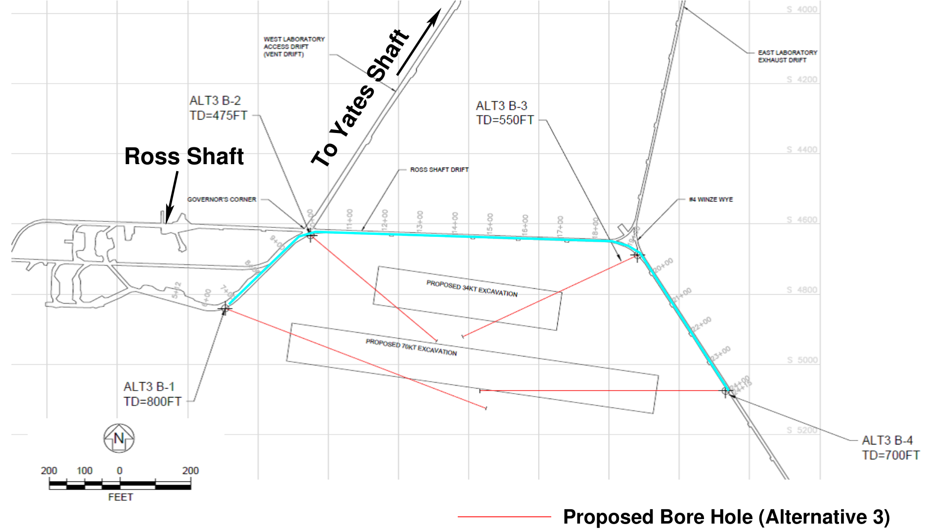
Neutrino Mixing, Mass
Hierarchy and CP Violation
4.1 Experimental Requirements Based on Oscillation Phenomenology
The experimental requirements for designing a neutrino oscillation experiment to simultaneously address neutrino CP violation and the mass hierarchy (MH) can be extrapolated as follows from the phenomenology summarized in Chapter 2:
- 1.
Phenomenology: An appearance experiment is necessary to extract the CP-violating effects.
Experimental requirements:
- •
The experiment will probe oscillations of .
- •
The experiment will identify and with high efficiency and purity in order to tag (or otherwise know) the flavor of the neutrino before and after flavor transformations.
- •
The experiment requires so that it will be possible to perform flavor-tagging of muon neutrinos using the lepton flavor produced in a charged current (CC) interaction ().
- •
- 2.
Phenomenology: In the three-flavor mixing model, the CP-violating Jarlskog invariant arises in the interference term as given by Equation 2.15; the oscillation scale where the interference term is maximal is that determined by the mixing between the and states.
Experimental requirements:
- •
The experimental baseline and corresponding neutrino energy are chosen according to Equation 2.18 such that equals to maximize sensitivity to the CP-violating term in the neutrino flavor mixing.
- •
Flavor-tagging of muon neutrinos that can be produced either at the source or after flavor-mixing requires ; therefore, the experimental baselines over which to measure neutrino oscillations are 11 1 Neutrino experiments using beams from pion decay-at-rest experiments such as DAEALUS are exceptions since the production spectrum is well known and only the flavor after oscillations is tagged through inverse-beta decay. The neutrino energies are below the CC muon-production threshold..
- •
- 3.
Phenomenology: In the three-flavor model oscillations depend on all parameters in the neutrino mixing matrix as well as on the mass differences, as shown in Equations 2.12 to 2.15.
Experimental requirements:
- •
The precision with which can be determined — and the sensitivity to small CP-violating effects or CP violation outside the three-flavor model — requires precision determination of all the other mixing parameters, preferably in the same experiment. The experiment will be designed so as to minimize dependence on external measurements of the oscillation parameters.
- •
- 4.
Phenomenology: Observation of CP violation requires the explicit observation of an asymmetry between and .
Experimental requirements:
- •
The experiment will probe the oscillations of both neutrinos and antineutrinos in an unambiguous way.
- •
The experiment will be capable of charge tagging in addition to flavor tagging. Charge tagging can be achieved at detection using the lepton charge and/or at production by selecting beams purely of neutrinos or antineutrinos.
- •
The experiment will be capable of resolving degeneracies between matter and CP asymmetries in order to determine the MH. This can be achieved by using a baseline greater than or with measurements probing oscillations over a range of values.
- •
- 5.
Phenomenology: CP asymmetries are maximal at the secondary oscillation nodes.
Experimental requirements:
- •
Coverage of the scale of the secondary oscillation nodes improves experimental sensitivity to small values of by enabling measurements of the asymmetry at the secondary nodes where the CP asymmetries are much larger and where there is no degeneracy with the matter asymmetries. The experiment will be performed with a wide-band beam to provide sensitivity to the scale of both the first and second oscillation nodes.
- •
The experimental baseline will be , given that muon flavor tagging is required at either production or detection. The secondary oscillation nodes are located at scales set by Equation 2.18 where . The second oscillation maximum is located at scales given by .
- •
Based on the experimental requirements prescribed by the neutrino oscillation phenomenology detailed above, pursuit of the primary science objectives for LBNE dictates the need for a very large mass () neutrino detector located at a distance greater than from the neutrino source. This large mass coupled with a powerful wide-band beam and long exposures is required to accumulate enough neutrino interactions — () events — to make precision measurements of the parameters that govern the subdominant oscillations. At , the baseline chosen for LBNE, both the first and second oscillation nodes are at neutrino energies , as shown in Figure 4.1. This places both neutrino oscillation nodes in a region that is well matched to the energy spectrum of the high-power conventional neutrino beams that can be obtained using the Main Injector (MI) proton accelerator at Fermilab.
4.2 Simulation of Neutrino Oscillation Experiments
To evaluate the sensitivity of LBNE and to optimize the experiment design, it is important to accurately predict the neutrino flux produced by the neutrino beamline, the neutrino interaction rate at the far detector, and the far detector performance. This is achieved using Monte Carlo (MC) simulations and the GLoBES [130, 131] package. The simulations and experimental assumptions that are used to evaluate the sensitivity of LBNE to neutrino mixing parameters, to the neutrino mass hierarchy (MH) and to CP violation are described in this section.
4.2.1 Expected Signal
The LBNE beamline design, described in Section 3.4, is simulated using Geant4 [132]. The simulated spectrum (unoscillated flux cross section) at obtained from the LBNE beamline using protons from the MI is shown as the black histogram in Figure 4.1. At this baseline, there is no degeneracy between matter and CP asymmetries at the first oscillation node where the LBNE neutrino beam spectrum peaks. The wide coverage of the oscillation patterns enables the search for physics beyond the three-flavor model because new physics effects may interfere with the standard oscillations and induce a distortion in the oscillation patterns. As a next-generation neutrino oscillation experiment, LBNE aims to study in detail the spectral shape of neutrino mixing over the range of energies where the mixing effects are largest. This is crucial for advancing the science beyond the current generation of experiments, which depend primarily on rate asymmetries.
The LBNE reconfiguration study [25] determined that the far detector location at the Sanford Underground Research Facility provides an optimal baseline for precision measurement of neutrino oscillations using a conventional neutrino beam from Fermilab. The baseline optimizes sensitivity to CP violation and is long enough to resolve the MH with a high level of confidence, as shown in Figure 2.7.
| Experiment | Baseline | unosc. | osc. | beam | CC | ||||
|---|---|---|---|---|---|---|---|---|---|
| details | km | CC | CC | CC | NC | CC | , | , | |
| LBNE LE | |||||||||
| 80 GeV, | |||||||||
| POT/year | |||||||||
| 50 | 12721 | 4339 | 108 | 3348 | 156 | 605 | 480 | 350 | |
| 50 | 4248 | 1392 | 34 | 1502 | 48 | 51 | 86 | 106 | |
| LBNE ME | |||||||||
| 120 GeV, | |||||||||
| POT/year | |||||||||
| 50 | 19613 | 12317 | 72 | 5808 | 686 | 435 | 399 | 293 | |
| T2K | 295 | ||||||||
| 30 GeV, | |||||||||
| POT/year | |||||||||
| 50 | 2100 | 898 | 41 | 360 | 73 | 58 | 39 | ||
| MINOS LE | 735 | ||||||||
| 120 GeV, | |||||||||
| POT/year | |||||||||
| 50 | 17574 | 11223 | 178 | 4806 | 115 | 345 | 326 | 232 | |
| 50 | 5607 | 3350 | 56 | 2017 | 32 | 58 | 85 | 88 | |
| NOvA ME | 810 | ||||||||
| 120 GeV, | |||||||||
| POT/year | |||||||||
| 50 | 4676 | 1460 | 74 | 1188 | 10 | 196 | 168 | 116 | |
| 50 | 1388 | 428 | 19 | 485 | 2 | 22 | 35 | 41 | |
| LBNO | |||||||||
| 50 GeV | |||||||||
| POT/year | |||||||||
| 50 | 8553 | 2472 | 48 | 2454 | 570 | 534 | 426 | 336 | |
| 50 | 3066 | 828 | 15 | 1140 | 255 | 24 | 45 | 54 | |
| -Factory | unosc. | osc. | CC | ||||||
| details | CC | CC | NC | CC | , | , | |||
| NuMAX I | |||||||||
| 3 GeV, | |||||||||
| /year | |||||||||
| 50 | 1039 | 339 | 484 | 28 | 71 | 97 | 117 | ||
| 50 | 2743 | 904 | 945 | 89 | 24 | 19 | 12 | ||
| NuMAX II | |||||||||
| 3 GeV, | |||||||||
| /year | |||||||||
| 50 | 6197 | 2018 | 2787 | 300 | 420 | 580 | 700 | ||
| 50 | 16349 | 5390 | 5635 | 534 | 139 | 115 | 85 | ||
Table 4.1 lists the beam neutrino interaction rates for all three known species of neutrinos as expected at the LBNE far detector. This table shows only the raw interaction rates using the neutrino flux from the Geant4 simulations of the LBNE beamline and the default interaction cross sections included in the GLoBeS package [130] with no detector effects included. A tunable LBNE beam spectrum, obtained by varying the distance between the target and the first focusing horn (Horn 1), is assumed. The higher-energy tunes are chosen to enhance the appearance signal and improve the oscillation fits to the three-flavor paradigm. To estimate the NC event rates based on visible energies above , a true-to-visible energy smearing function based on output from the GENIE neutrino MC generator [133] is used. For comparison, the rates at current neutrino oscillation experiments such as T2K [134], MINOS [135] and NOA [126] are shown for similar exposure in mass and time and using the same interaction cross sections. The raw interaction rates from other proposed neutrino oscillation experiments such as LBNO [136] and the NuMAX neutrino factory designs [137] are also shown22 2 T2K uses a JPARC neutrino beam, MINOS and NOA use the Fermilab NuMI neutrino beam and LBNO uses a CERN neutrino beam.. It is important to note that the duty factors for the JPARC and CERN beams are and of NuMI/LBNE respectively. For LBNO, the event rates are obtained using the optimized beam from the HP-PS2 synchrotron [138] with an exposure of . The LBNO duty cycle is assumed to be seconds/year, which corresponds to a beam power of . Note that for Stage 1 and Stage 2 of the NuMAX neutrino factory proposal [137], Project X beams [23] at 3 GeV with 1 and 3 MW, respectively, are needed33 3 Project X has been superseded by PIP-II as of late 2013; PIP-II is briefly described in Section 3.4. It is clear that the LBNE beam design and baseline produce high rates of appearance coupled with large rate asymmetries when CP-violating effects are included. For example, LBNE has significantly higher appearance rates with a Main Injector beam when compared to Stage 1 of the NuMAX neutrino factory with a beam from a linac. The appearance rates are very similar in LBNE and LBNO with normal hierarchy (NH), but the appearance rates (NH) in LBNO are that of LBNE due to the suppression from the larger matter effect (longer baseline) in LBNO.
4.2.2 Detector Simulation using the GLoBES Package
For the sensitivity studies presented here, the GLoBES package [130, 131] was used to simulate the detector response using simple smearing and using detector efficiency values based on results from ICARUS and earlier simulation efforts as documented in [29]. The values used in GLoBES are shown in Table 4.2.
| Parameter | Range of Values | Value Used for LBNE Sensitivities |
|---|---|---|
| For -CC appearance studies | ||
| -CC efficiency | 70-95% | 80% |
| -NC misidentification rate | 0.4-2.0% | 1% |
| -CC misidentification rate | 0.5-2.0% | 1% |
| Other background | 0% | 0% |
| Signal normalization error | 1-5% | 1-5% |
| Background normalization error | 2-15% | 5-15% |
| For -CC disappearance studies | ||
| -CC efficiency | 80-95% | 85% |
| -NC misidentification rate | 0.5–10% | 1% |
| Other background | 0% | 0% |
| Signal normalization error | 1-10% | 5–10% |
| Background normalization error | 2-20% | 10-20% |
| For -NC disappearance studies | ||
| -NC efficiency | 70-95% | 90% |
| -CC misidentification rate | 2-10% | 10% |
| -CC misidentification rate | 1-10% | 10% |
| Other background | 0% | 0% |
| Signal normalization error | 1-5% | under study |
| Background normalization error | 2-10% | under study |
| Neutrino energy resolutions | ||
| -CC energy resolution | ||
| -CC energy resolution | ||
| scale uncertainty | under study | under study |
| scale uncertainty | 1-5% | 2% |
Studies from ICARUS have estimated and measured single-particle energy resolutions in liquid argon. Below , the energy resolution of electrons is . The energy resolution of an electromagnetic shower with energy in the range (50–5000) MeV is [139] and that of hadronic showers is . A significant fraction of the -CC signal in LBNE in the range of comes from non-quasi-elastic CC interactions with a large component of the visible energy in the hadronic system. From recent simulations of neutrino interactions in this region it has been determined that . For this reason, the total energy resolution for the neutrino oscillation sensitivity calculation is chosen to be . In a non-magnetized LArTPC, the muon momentum can be obtained from measurements of range and multiple scattering. The muon momentum resolution for partially contained muons is found to be in the range [140, 141] for muons in the range. The total energy resolution in LBNE is, therefore, assumed to be ; the resolution will be significantly better than this for the small subsample of events in which muons are fully contained by the detector.
| Beam | Hierarchy | Signal Events | Background Events | ||||
| CC | NC | CC | Beam | CC | Total | ||
| (disappearance) | |||||||
| Neutrino | - | 2056/96 | 23 | N/A | - | 18 | 41 |
| Antineutrino | - | 280/655 | 10 | N/A | - | 10 | 20 |
| (appearance) | |||||||
| Neutrino | Normal | 229/3 | 21 | 25 | 47 | 14 | 107 |
| Neutrino | Inverted | 101/5 | 21 | 25 | 49 | 17 | 112 |
| Antineutrino | Normal | 15/41 | 11 | 11 | 24 | 9 | 55 |
| Antineutrino | Inverted | 7/75 | 11 | 11 | 24 | 9 | 55 |
Figures 4.2 and 4.3 show the predicted spectra of observed signal and background events in LBNE produced from the GLoBES implementation, including the effects of neutrino oscillation. Figure 4.2 shows the and -CC sample and Figure 4.3 shows the and -CC appearance sample. Table 4.3 shows the expected LBNE signal and background event rates in disappearance and appearance modes for neutrinos and antineutrinos, for normal (NH) and inverted (IH) hierarchy. The rates are given per of fiducial LArTPC mass.
The GLoBES implementation used in the sensitivity studies presented here appears to be in good agreement with more recent results from the Fast MC, described in Section A.3. Updated sensitivity and systematics studies are currently underway using the Fast MC for detector simulation, and customized GLoBES-based software for the oscillation fits and propagation of systematics. A full MC simulation of the far detector and automated event reconstruction is being developed; this is also described in Appendix A.
4.3 Measurements of Mass Hierarchy and the CP-Violating Phase
The neutrino mass hierarchy (MH) and the value of the CP-violating phase, , are currently unknown. Knowledge of the MH has significant theoretical, cosmological and experimental implications. A determination of the value to be neither zero () nor would constitute the first observation of CP violation in the lepton sector.
The expected performance of a LArTPC far detector downstream from a neutrino source is detailed in the LBNE Conceptual Design Report Volume 1 [29]. Estimated sensitivities to the determination of the MH and discovery of CP violation, presented both here and in the CDR, are calculated using the GLoBES package. The detector response assumed in these calculations is summarized in Table 4.2. The sensitivities are obtained by simultaneously fitting the , , , and oscillated spectra, examples of which are shown in Figures 4.2 and 4.3. The background is not used in the sensitivity calculations since it is expected that further analysis will reduce this background to negligible levels.
In these calculations, experimental sensitivity is quantified using parameters, which are determined by comparing the predicted spectra for various scenarios. These quantities are defined, differently for neutrino MH and CP-violation sensitivity, to be:
| (4.1) | |||||
| (4.2) | |||||
| (4.3) |
These sensitivities are evaluated separately for true NH and IH. Since the true value of is unknown, a scan is performed over all possible values of . The individual values are calculated using
| (4.4) |
where n are event rate vectors in bins of reconstructed energy and represents a nuisance parameter to be profiled. Nuisance parameters include the values of mixing angles, mass splittings, and signal and background normalization. The nuisance parameters are constrained by Gaussian priors; in the case of the oscillation parameters, the Gaussian prior has standard deviation determined by taking 1/6 of the 3 range allowed by the global fit [54].
With the exception of results reported in Section 4.3.1, where more information on the statistical interpretation of MH sensitivity is provided, the sensitivities presented here are for the typical experiment with no statistical fluctuations considered. In the absence of statistical fluctuations, the value for the true spectra is identically zero. Statistical fluctuations are incorporated by repeatedly varying the contents of each energy bin in each sample by drawing from a Poisson distribution with the expected number of events in that bin as the mean.
This section presents the sensitivities of various LBNE configurations to determination of the MH and CP violation. In particular, a far detector and the full-scope far detector are considered. In each case, the performance of LBNE with both the beamline design presented in the CDR [30] as well as the upgraded beam described in Section 3.4 is studied. In addition, the sensitivities at different possible stages of LBNE with increases to far detector mass and Main Injector beam upgrades are estimated.
Figure 4.4 summarizes the sensitivities for determining the MH and CP violation () as a function of the true value of with a LArTPC. The red band shows the sensitivity that is achieved with an exposure of six years with equal exposures in and mode in a beam. The cyan band shows the sensitivity obtained by combining the LBNE with T2K and NOA, where the T2K exposure is POT in mode only and the NOA exposure is six years (assuming POT per year) with equal exposures in and mode. The bands indicate the sensitivity range corresponding to different levels of signal and background normalization uncertainties and different possible beam designs. The gray curves are the expected sensitivities for the combination of NOA and T2K. The known mixing parameters are allowed to float in the fit, but are constrained (using a Gaussian prior) by the uncertainties from the 2012 global best fit [54]. The reactor mixing angle, , is constrained to be . The uncertainty is equal to the size of the current systematic uncertainty from the Daya Bay Experiment [142] and is used as a conservative estimate of the precision that will be achieved by the current generation of reactor experiments. Figure 4.5 shows the sensitivities for determining the MH and CP violation as a function of the true value of after six years of running in the LBNE configuration under the same assumptions.
The sensitivity bands in Figures 4.4 and 4.5 represent the variation in sensitivity as a function of the beam design and normalization uncertainties on the signal and background. The solid curve at the lower end of the red band represents the beamline design described in the LBNE CDR Volume 2 [30] for which there is no near detector. The dashed line above the solid curve represents the sensitivity with the beam design improvements currently under study as described in Section 3.4, still without a near detector. The dashed line at the upper end of the red band represents the case in which both the beam design improvements and a high-resolution, highly capable near detector are implemented. The key design goal of the LBNE near detector and beamline simulation software is to enable a prediction of the far detector unoscillated flux with a precision of . Therefore, the total signal and background normalization uncertainties on the disappearance signal are assumed to be 5% and 10%, respectively. The default appearance signal uncorrelated normalization uncertainties for the full-scope LBNE presented in this chapter are assumed to be 1%. The appearance background uncertainty is expected to be at least as good as the [143] achieved by the appearance search in the MINOS experiment.
A detailed discussion of the systematics assumptions for LBNE is presented in Section 4.3.2. In the case that LBNE has no near neutrino detector, the uncertainties on signal and background are expected to be and , respectively, extrapolating from the performance and detailed knowledge of the NuMI beam on which the LBNE beamline is modeled, in situ measurements of the muon flux at the near site as described in [29], the expectation of improved hadron production measurements with the NA61 and MIPP experiments, and the experience of previous appearance experiments as summarized in Table 4.4.
| Experiment | Year | -NC/CC | -CC | Background | Comment |
| Events | Events | Syst.Error | |||
| BNL E734 [144] | 1985 | 235 | 418 | 20% | No ND |
| BNL E776(NBB) [145] | 1989 | 10 | 9 | 20% | No ND |
| BNL E776 (WBB) [146] | 1992 | 95 | 40 | 14% | No ND |
| NOMAD [147] | 2003 | 300 | 5500 | % | No ND |
| MiniBooNE [148] | 2008 | 460 | 380 | 9% | No ND |
| MiniBooNE [49] | 2013 | 536 | 782 | 5% | SciBooNE |
| MINOS [143] | 2013 | 111 | 36 | 4% | ND–FD |
| T2K [149] | 2013 | 1.1 | 26 | 9%* | ND–FD |
4.3.1 Interpretation of Mass Hierarchy Sensitivities
In the mass hierarchy (MH) determination, only two possible results are considered, as the true MH is either normal (NH) or inverted (IH). Reference [150] presents the statistical considerations of determining the sensitivity of an experiment to the MH, framed partly in the context of two separate but related questions:
- 1.
Given real experimental data, with what significance can the MH be determined?
- 2.
When evaluating future experimental sensitivities, what is the probability that a particular experimental design will be able to determine the MH with a given significance?
Once data are in hand, a number of techniques based either within Bayesian or frequentist statistics make it possible to determine the level of confidence at which one MH hypothesis or the other can be ruled out. In assessing the sensitivity of future experiments, it is common practice to generate a simulated data set (for an assumed true MH) that does not include statistical fluctuations. The expected sensitivity can be reported as , representative of the mean or the most likely value of that would be obtained in an ensemble of experiments for a particular true MH. With the exception of Figure 4.7, the sensitivity plots in this document have been generated using this method.
However, addressing the expected sensitivity of an experiment per the second question above requires consideration of the effect of statistical fluctuations and variations in systematics. If the experiment is repeated many times, a distribution of values will appear. Studies in [150] and elsewhere (e.g., [151]) show that the metric employed here does not follow the commonly expected function for one degree of freedom, which has a mean of and can be interpreted using a Gaussian distribution with a standard deviation of . Rather, these studies show that when the observed counts in the experiment are large enough, the distribution of used here approximately follows a Gaussian distribution with a mean and standard deviation of and , respectively [150].
Figure 4.6 shows the expected distribution of values in LBNE from toy Monte Carlo studies.
The interpretation of pairs of distributions, such as those in the various panels of this figure, depends on the information being sought. For example, one is not necessarily interested simply in the fraction of experiments where has the “right” sign. (An experiment that obtains a small value of , even with the “right” sign, would not be particularly constraining since there is no way a priori to know which is the right sign — this is what the experiment is attempting to measure.) It should also be noted that in general , i.e., true NH, is not necessarily equal to , i.e., true IH, nor do the corresponding distributions necessarily have the same shape. For some ranges in , for example, the event rate in LBNE is sufficiently different for the two MH hypotheses that the corresponding distributions in are quite distinct.
The plots shown on the left in Figure 4.6 illustrate the case for a true value of , where the distributions for NH and IH scenarios are similar. Shown on the right are the corresponding distributions for the case of , where for NH the matter asymmetry is maximally offset by the CP asymmetry, leading to poorer MH discrimination. For the IH case, these effects go in the same direction, leading to better MH discrimination. The converse is the case for . Since the true value of is unknown (although a best-fit value and confidence interval will emerge from the analysis of the data collected), comparison of a given value of with expected distributions for NH and IH cases for the same value of does not in general provide the appropriate test. For simplicity, following [151], the discussion below focuses on the respective values of for which the experiment will have poorest sensitivity for NH () and IH () scenarios.
Given the above introduction to the statistical fluctuation issues, it is natural to employ the statistical language of hypothesis testing in projecting LBNE’s MH sensitivity. Specifically, is defined as the desired Type-I error rate — that is, the probability of rejecting a particular hypothesis, e.g., NH, in the case where this is the true hypothesis. One can then ask what the corresponding Type-II error rate would be, defined as the probability of accepting the hypothesis being tested (NH in this example), when in fact the alternate hypothesis (IH) is true. The pair of and would correspond to a particular value of chosen (in advance of the experiment) as a criterion for deciding whether to rule out the NH (or IH). Historically, many experiments have characterized their anticipated sensitivity by reporting for the case of , which is nothing more than that given by the median value of the test statistic (in this case, ) as described above. Sometimes, the sensitivity is also reported as the square root of .
Due to the approximate symmetry of the MH ambiguity as a function of for the two MH scenarios and the desire to be able to reject exactly one of the two possible mass orderings [151], it is also natural to report a value of for an experiment such that [152, 153, 151]. In this way, it is possible to express just how unlucky an experiment can be while maintaining a corresponding sensitivity . In the case of LBNE, a reasonable benchmark for comparison corresponds to . For this case, specifying yields , which means that the experiment will have a 0.13% probability of ruling out the true MH hypothesis and of accepting the wrong MH hypothesis.
As described above, and as is evident in the plots presented, such as those in Figures 4.4 and 4.5, the sensitivity of LBNE is strongly dependent on the true value of ; Figure 4.7 shows that it also depends on the true value of . While plotting the value of (for some choice of , such as or ) as a function of these parameters encapsulates the sensitivity, a visually helpful presentation is obtained by plotting the expected mean value, , as well as ranges of possible values corresponding to the expected distribution in . Thus, Figure 4.7 shows the dependence of on the true value of for the typical LBNE data set, for two possible values of , as well as the corresponding expectation bands within which 68% (green) and 95% (yellow) of LBNE sensitivities will fall. These expectation bands give a semi-quantitative picture of the likely range of outcomes for the experiment.
The horizontal dashed lines on Figure 4.7 specify the confidence level of an experiment with a particular value of such that:
| (4.5) |
following the convention in [150], where the notation represents the probability of A given condition B, and these probabilities are inferred from the corresponding likelihoods via Bayes’ Theorem. Alternatively, the values shown in these plots can be approximately translated to sensitivities in terms of , for whatever choice of is desired, following, for example, the prescription described in [151].
As seen in Figure 4.7, a typical LBNE data set with a detector can determine the MH with for all values of (for the left plot, where ). From a Bayesian analysis, the probability that an experiment measuring has ruled out the true MH hypothesis is , as indicated for the corresponding horizontal dashed line in the plots in this figure. When considering the effect of statistical fluctuations, for the same value of , about 97.5% of experiments will determine the MH with for the least favorable value of , where corresponds to a CL of 98.9%.
For the bulk of the range of , the sensitivity of LBNE is vastly better than for the least favorable value described above. Furthermore, newer data prefer values of closer to maximal [69], which results in significantly enhanced LBNE MH sensitivity. As shown in the right-hand plot of Figure 4.7, if , the expected MH sensitivity for the typical LBNE experiment at the least favorable point is , which is significantly larger than the sensitivity of expected for the same value of if . This suggests that a typical LBNE data set will determine the MH with well above the benchmark value of mentioned above for even the least favorable values of .
4.3.2 Sensitivities and Systematics
The main systematic uncertainties in any experiment are determined by the analysis strategy employed and the performance of the detector. Figure 4.8 outlines the analysis strategy commonly employed to extract oscillation parameters in two-detector long-baseline neutrino oscillation experiments.
The measured spectrum of events in the near detector, is extrapolated to the far detector and is used to predict both the and appearance signals in the far detector, and respectively. The measured spectrum of candidates in the near detector, , which comprises mostly the beam events and NC misidentified events, is used to predict the background to the appearance signal in the far detector. In LBNE, neutrino oscillation parameters will be extracted using a fit to four far detector data samples: , , , and , which will allow for partial cancellation of uncertainties.
In the current generation of experiments, the measured spectrum of neutrino events in the near detector is a product of beam flux (), detector efficiency and smearing (), and neutrino interaction dynamics (). To extrapolate the observed spectra in the near detector to the far detector, corrections have to be made for:
- 1.
Differences in the beam flux in the near and far detectors, : The near detector is much closer to the neutrino beamline and sees an extended source of neutrinos from the decay pipe as compared to the far detector, which observes a point source. A beam MC is used to correct for these differences. Uncertainties arise from inaccuracies in the simulation of the hadron production from the target, the focusing of the horns, the material in the beamline (which absorbs hadrons before they can decay), and the decay channel geometry.
- 2.
Differences in near and far detector smearing and efficiencies, : The largest uncertainties arise from the different event selection efficiencies in the near and far detectors and, in particular, the imperfect modeling of the energy scales of the near and far detectors. Identical near and far detectors allow most of these uncertainties to cancel in the extrapolation in the case of the signal prediction. The signal prediction is extrapolated from ; thus there are irreducible residual uncertainties arising from different criteria used to select and candidate events and different detector response functions.
- 3.
Differences in the interactions of neutrinos in the near and far detector, : In the case in which both near and far detectors use the same target nucleus, the differences cancel for extrapolation of the signal from the near to the far detector. When using the signal in the near detector to predict the (and ) signals in the far detector, uncertainties arising from differences in () and interactions, , dominate. These uncertainties are limited by theoretical uncertainties and are typically smaller at higher energies.
The estimation of the expected signals at the far detector can be summarized thus:
| (4.6) | |||||
| (4.7) |
| (4.8) | |||||
Expected systematic uncertainties on the LBNE appearance and signal samples in the three-flavor fit for LBNE (Table 4.2) are extrapolated from the current performance of the MINOS [143, 154] and T2K [149] experiments. The dominant uncertainties on the current appearance analysis from MINOS and T2K and the expected corresponding uncertainties in LBNE are shown in Table 4.5.
| Source of | MINOS | T2K | LBNE | Comments |
| Uncertainty | Absolute/ | |||
| Beam Flux | 3%/0.3% | 2.9% | 2% | MINOS is normalization only. |
| after N/F | LBNE normalization and shape | |||
| extrapolation | highly correlated between . | |||
| Detector effects | ||||
| Energy scale | 7%/3.5% | included | (2%) | Included in LBNE sample |
| () | above | uncertainty only in three-flavor fit. | ||
| MINOS dominated by hadronic scale. | ||||
| Absolute energy | 5.7%/2.7% | 3.4% | 2% | Totally active LArTPC with calibration |
| scale () | includes | and test beam data lowers uncertainty. | ||
| all FD | ||||
| effects | ||||
| Fiducial | 2.4%/2.4% | 1% | 1% | Larger detectors = smaller uncertainty. |
| volume | ||||
| Neutrino interaction modeling | ||||
| Simulation | 2.7%/2.7% | 7.5% | Hadronization models are better | |
| includes: | constrained in the LBNE LArTPC. | |||
| hadronization | N/F cancellation larger in MINOS/LBNE. | |||
| cross sections | X-section uncertainties larger at T2K energies. | |||
| nuclear models | Spectral analysis in LBNE provides | |||
| extra constraint. | ||||
| Total | 5.7% | 8.8% | 3.6 % | Uncorrelated uncertainty in |
| full LBNE three-flavor fit = 1-2%. | ||||
The categorization of the dominant experimental uncertainties in Table 4.5 are not always in exact correspondence since T2K and MINOS are very different experiments and deploy different analysis techniques. A detailed description of the expected LBNE performance on each of the dominant uncertainties follows.
Beam flux uncertainties: The LBNE high-resolution near detector is being designed with the goal of accurately measuring the unoscillated beam flux at the near site with a precision for both shape and absolute normalization. Table 4.6 summarizes the precision that can be achieved using different near detector analysis techniques, described in detail in Section 7.1, to measure the absolute normalization and shape of the different components of this flux.
| Technique | Flavor | Absolute | Relative | Near Detector |
| normalization | flux | requirements | ||
| NC Scattering | 2.5% | ID | ||
| Resolution | ||||
| Separation | ||||
| Inverse muon | 3% | ID | ||
| decay | Resolution | |||
| 2-Track (X) Resolution | ||||
| energy scale | ||||
| CC QE | target | |||
| Angular resolution | ||||
| energy resolution | ||||
| Back-Subtraction | ||||
| CC QE | target | |||
| Back-Subtraction | ||||
| Low- | 2.0% | vs | ||
| -Scale | ||||
| Low- Resolution | ||||
| Low- | 2.0% | vs | ||
| -Scale | ||||
| Low- Resolution | ||||
| Low- | / | 1-3% | 2.0% | Separation () |
| CC | / | <1% | 2% | ID & ID |
| / Resolution | ||||
| CC | / | <1% | 2% | ID & ID |
| / Resolution | ||||
| Low-/CohPi | / | 2% | 2% | ID & ID |
| Resolution | ||||
| Resolution |
It is important to note that several of these techniques have already been used and proven to work in neutrino experiments such as MINOS [155] and NOMAD [156, 157]. In particular, the inclusive neutrino charged current (CC) cross-section measurement in the MINOS near detector reported in [155] has already achieved a normalization uncertainty of in the range of GeV using the low- method described in Section 7.1. The total systematic uncertainty on the NuMI neutrino flux determination by the MINOS near detector reported in [155] was and was limited by the detector performance. Recent independent studies on extraction of the neutrino flux using the low- method [158] indicate that the technique can be reliably extended down to .
The LBNE near detector is being designed to significantly improve performance relative to the current generation of high-intensity neutrino detectors. A detailed beamline simulation will enable the extrapolation of the LBNE near detector flux measurements to the unoscillated far detector spectrum with high precision using techniques similar to those used by MINOS [159]. The near-to-far unoscillated-spectrum extrapolation uncertainties already achieved by MINOS are in the MINOS (and also in the LBNE) appearance signal range of [160, 159]. The MINOS extrapolation does not include any independent constraints on the hadron production spectrum from the proton target or information on the horn focusing performance from the muon flux measurements at the near site. The NuMI beamline — the design of which is very similar to LBNE’s — is expected to operate for more than a decade with improved flux measurements using the much more capable MINERA detector [161] in both the low-energy and high-energy tunes. MINERA is designed to measure the absolute NuMI flux with a precision of or better; data from MINERA will be used to further improve the accuracy of the LBNE beamline simulation, reducing the uncertainties on the extrapolation of the flux. A new program of hadron production measurements at the NA61/SHINE [162] experiment will also reduce the near-to-far extrapolation uncertainties from the LBNE beamline simulation. The combination of LBNE near detector flux measurements and improved beamline simulation is expected to enable a prediction of the far detector appearance signal with a precision of % total normalization and shape uncertainty. Since this uncertainty is highly correlated among the four data samples in the three-flavor fit, the final uncorrelated uncertainty on the signal sample will be significantly smaller.
energy-scale uncertainty: Both T2K and MINOS use the reconstructed event spectrum in the near detector to predict the appearance signal at the far detector. Therefore the energy-scale uncertainty in the near detector is propagated as an uncertainty on the appearance signal at the far detector. In MINOS — which has a high proportion of non-QE events — the energy-scale uncertainty is dominated by uncertainty in the hadronic energy scale (7% for GeV) [163] and the muon energy scale (2.5%). Utilization of the low- method for energies less than 3 GeV in LBNE reduces the hadronic energy-scale contribution to the uncertainty in the energy scale in the near detector. As discussed in Chapter 7, it is expected that both the muon and hadronic energy-scale uncertainties in the near detector will be 1%, so far detector energy-scale uncertainties will dominate the uncertainty in the signal prediction. The high-resolution LArTPC far detector and an active program of hadron test-beam experiments planned for LBNE will reduce far detector hadronic energy-scale uncertainties, which also contribute to uncertainty in the energy scale of the far detector signal used in the three-flavor analysis. Extrapolating from MINOS, the LBNE energy-scale uncertainty is thus estimated to be .
In MINOS, the 7% energy-scale uncertainty resulted in a residual uncertainty of 3.5% on the signal prediction. In the LBNE full three-flavor analysis, this uncertainty is 100% correlated between the predicted and signal samples; therefore a energy-scale uncertainty of 2% is assigned to the signal prediction in LBNE. The residual uncorrelated uncertainty on the signal prediction is considered to be negligible.
Absolute energy-scale uncertainties: In Figure 4.9, the MH and CP-violation sensitivity obtained using a rate-only, a shape-only and a rate+shape analysis of appearance is shown. This study demonstrates that a critical component of LBNE’s oscillation sensitivity is an accurate measurement of the shape of the appearance signal.
This measurement depends on the precision with which the detector response to interactions is understood. The energy-scale uncertainty, which is not yet included in the current sensitivity calculation with the GLoBES framework, is therefore expected to be an important systematic uncertainty in the LBNE oscillation analysis.
The effect of energy-scale uncertainty on the signal normalization, determined by the precision of detector calibration, was 2.7% in MINOS and 3.4% in T2K, where the T2K uncertainty actually includes most far detector effects. LBNE’s LArTPC detector technology is expected to outperform both the MINOS sampling calorimeter and the T2K water Cherenkov detector in reconstruction of the interaction. For example, the proton produced from the -QE interaction — the interaction with potentially the best energy resolution — is clearly visible in a LArTPC [164], whereas it is often below Cherenkov threshold in T2K. An active program of test beam experiments with LArTPCs is currently being planned to address the detector response to electrons and hadrons. Results from the test beam experiments and the projected performance of the in situ calibration will enable LBNE to limit the detector energy-scale uncertainties below the level achieved by the current generation of experiments.
Hadronic energy is expected to contribute more than half of the total energy deposit for many and interactions in LBNE. The hadronic energy scale does not depend on neutrino flavor; since it should be identical for and interactions, this portion of the absolute energy-scale uncertainty is expected to largely cancel in the LBNE three-flavor analysis. This cancellation may be reduced to the extent that event-selection criteria vary the hadronic energy fraction among the samples.
Simulation uncertainties: The simulation uncertainties listed in Table 4.5 refer primarily to uncertainties in modeling neutrino interactions with the target nucleus in the near and far detectors. These uncertainties include and cross-section uncertainties, uncertainties arising from the modeling of the structure of the target nucleus, modeling of final-state interactions within the nucleus, and hadronization model uncertainties arising from the break up of the target nucleus in higher-energy inelastic interactions. The deployment of identical nuclear targets in the MINOS (iron) and LBNE (argon) near and far detectors allows for a larger cancellation of the simulation uncertainties as compared to T2K, which used dissimilar target nuclei in its near detector (carbon) and far detector (oxygen). A high-resolution near detector such as that being designed for LBNE will enable further constraints on the hadronization models by resolving many of the individual particles produced in resonance and deep inelastic interactions, which represent 75% of LBNE neutrino interactions.
The MINOS appearance analysis achieved a 2.7% residual uncertainty from simulation after the near-to-far extrapolation. The MINOS simulation uncertainty is dominated by hadronization uncertainties, because cross-section uncertainties largely cancel between the identical nuclei in the near and far detectors. The T2K residual uncertainty after near-to-far extrapolation is 7%. Additionally, the T2K analysis includes more sources of cross-section uncertainties than MINOS and, at the lower T2K energies, larger differences in / cross sections (2.9 %) persist after extrapolating the spectrum in the near detector to the signal prediction in the far.
The LBNE near detector design is required to achieve a cancellation of near-to-far cross-section and hadronization-model uncertainties at the same level as MINOS or better. The appearance signal in LBNE peaks at ; these higher energies will result in lower uncertainties from the cross-section effects considered by T2K. In addition, since cross-section variations impact the observed and spectra differently when compared to oscillation effects, the fit to the wide-band spectrum in LBNE could constrain some of these uncertainties further. Therefore, it is expected that LBNE could reduce the total appearance simulation uncertainties to a level of 2%. Preliminary results from the LBNE Fast MC simulation (described in Section A.3) indicate that many cross-section uncertainties cancel out when combining the disappearance and appearance signal samples in a three-flavor fit, resulting in a much smaller uncorrelated uncertainty on the signal sample.
It is important to note that some simulation uncertainties may not cancel out in the near-to-far extrapolation or in the combined fit; in particular, uncertainties due to nuclear models and intra-nuclear effects are different for interactions. New models of intra-nuclear effects are being evaluated to determine the size of these irreducible residual uncertainties. Additionally, there are uncertainties at the level of 1-2% in the cross sections that will not cancel between and [165]. In the absence of theoretical progress, these should also be considered irreducible.
Fiducial volume uncertainties: One of the dominant uncertainties in the MINOS disappearance analysis — a high-precision oscillation analysis based on a detailed spectral shape — was the fiducial-volume uncertainty, which included near and far detector reconstruction uncertainties. The uncertainty on the fiducial volume of the MINOS far detector alone was 2.4%. T2K, with a much larger far detector ( fiducial), was able to reduce this uncertainty to the 1% level. It is expected that LBNE will be able to achieve this level of uncertainty on the appearance signal. With the combination of all four signal samples () in a three-flavor fit, the uncorrelated portion of this uncertainty is expected to be smaller than 1%.
appearance background systematic uncertainties: The appearance normalization uncertainty is expected to be at least as good as the [143] achieved by the appearance search in the MINOS experiment, using the technique of predicting intrinsic-beam and neutral current (NC) background levels from near detector measurements. The LBNE far detector should be able to provide additional constraints on the background level by independently measuring NC and background.
In Figure 4.10, the MH and CP-violation sensitivities as a function of exposure are evaluated using three different sets of assumptions regarding the uncorrelated signal/background normalization uncertainties: 1%/5% (the goal of the LBNE scientific program), 2%/5% and 5%/10%. The last is a conservative estimate of the uncertainties that can be achieved in LBNE without unoscillated neutrino beam measurements at the near site. The impact of signal and background normalization uncertainties on the MH sensitivity is small even at high exposures given the large asymmetry at and the fact that much of the sensitivity to the MH comes from analysis of the spectral shapes (Figure 4.9). For CP violation, however, the impact of normalization uncertainties is significant at exposures s.
| Systematic uncertainty | CPV Sensitivity | Required Exposure | |
| Fraction | () | ||
| 0 (statistical only) | 50% | 3 | |
| 50% | 5 | ||
| 1%/5% (Sig/bkgd) | 50% | 3 | |
| 50% | 5 | ||
| 2%/5% (Sig/bkgd) | 50% | 3 | |
| 50% | 5 | ||
| 5%/10% (no near det.) | 50% | 3 | |
Table 4.7 summarizes the LBNE exposures required to reach and sensitivity to CP violation for at least 50% of all possible values of . The exposures vary depending on the assumptions made about the normalization uncertainties that can be achieved in LBNE. The normalization uncertainty assumptions range from 1-2%/5% on signal/background to 5%/10%. The uncertainties listed in Table 4.7 and shown in the sensitivity figures pertain to the appearance signal and background normalization. In Figure 4.9 the sensitivities obtained from the rate only, shape only and rate+shape of the appearance spectrum are shown for a detector with an beam. For CP violation (right), the rate information dominates the sensitivity, but the shape information enables the detector to exceed sensitivity for large CP violation. For the MH sensitivity, Figure 4.9 (left) demonstrates that the sensitivity in the least favorable range of values is dominated by the shape information. Further analysis has shown that it is the region of the second oscillation node that is responsible for this effect. The shape of the signal in this region will enable LBNE to determine the sign of , which is sufficient to break the degeneracy with MH effects and determine the correct sign of the mass ordering.
Figures 4.11, 4.12, and 4.13 show the variation in sensitivity to CP violation and MH when the true value of the oscillation parameters , and are varied within the 3 range allowed by the 2012 global fit [54]. These sensitivities are calculated for six years with equal exposures in and mode in a beam for the case in which an upgraded beam and a near detector have both been implemented.
In comparing Figures 4.11, 4.12 and 4.13, the dependence on the true value of is particularly striking. As increases, the sensitivity to CP violation decreases because the CP asymmetry that LBNE measures is inversely proportional to as demonstrated in Equation 2.20. For the same reason, as increases, the degeneracy between the CP and matter asymmetries is broken, which increases the LBNE sensitivity to neutrino MH. The explicit dependence of MH sensitivity on the value of is shown in Figure 4.14.
As this plot makes clear, LBNE resolves the MH with a significance of for nearly all allowed values of and .
4.3.3 Summary of CP-Violation and Mass Hierarchy Sensitivities
For the LBNE, the statistical uncertainties are much larger than the systematic uncertainties. Combining the sensitivity from the LBNE with expected knowledge from the NOA and T2K experiments would allow LBNE to achieve a sensitivity for detecting CP violation for of the allowed values of and a sensitivity for of these values. It is clear that the LBNE sensitivity would be the dominant contribution in the combined sensitivities and would therefore represent a significant advance in the search for leptonic CP violation over the current generation of experiments, particularly in the region where the CP and matter effects are degenerate.
The combination with T2K and NOA would allow the MH to be determined with a minimum precision of over 60% values and for all possible values of . Due to the low event statistics in these experiments, the combination with NOA and T2K only helps the sensitivity in the region of (NH) or < 0 (IH) where there are residual degeneracies between matter and CP-violating effects. As will be discussed in Section 4.6, the combination with atmospheric neutrino oscillation studies can also be used to improve the MH sensitivity in this region for the LBNE configuration.
Table 4.8 summarizes the MH and CP sensitivities that can be reached by a typical experiment with the LBNE and configurations assuming a running time of 3+3 () years with a beam under a variety of scenarios.
| Scenario () | MH sensitivity | CPV sensitivity | ||
|---|---|---|---|---|
| Fraction | () | Fraction | () | |
| LBNE , CDR beam | 50% | 40% | ||
| 100% | - | - | ||
| LBNE , upgraded beam | 50% | 23% | ||
| 100% | 55% | |||
| LBNE , beam, with ND | 50% | 33% | ||
| 100% | 60% | |||
| + NOA (6 yrs), T2K ( POT) | 75% | 30% | ||
| 100% | 50% | |||
| LBNE , CDR beam | 50% | 20% | ||
| 100% | 50% | |||
| LBNE , upgraded beam | 50% | 15% | ||
| 100% | 35% | |||
| LBNE , beam, with ND | 50% | 35% | ||
| 100% | 50% | |||
4.3.4 CP-Violating and Mass Hierarchy Sensitivities with Increased Exposures
Figure 4.16 shows the minimum significance with which the MH can be resolved and CP violation determined by LBNE as a function of increased exposure in units of mass beam power time44 4 Time is denoted in years of running at Fermilab. One year of running at Fermilab corresponds to seconds.. For this study, the LBNE beamline improvements discussed in Section 3.4 are used with , and the signal and background normalization uncertainties are assumed to be 1% and 5%, respectively. Both and appearance signals are used in a combined analysis.
Due to the long baseline, the determination of the MH in LBNE to high precision does not require a large exposure; a sensitivity of for the worst case (NH, or IH, ) requires an exposure of s, but sensitivity can be reached for of the allowed values of with an exposure of less than s. On the other hand, reaching discovery-level sensitivity () to leptonic CP violation for at least 50% of the possible values of will require large exposures of s. Figure 4.17 demonstrates the sensitivity to CP violation as a function of and exposure that can be achieved with various stages of the Fermilab Proton-Improvement-Plan (PIP-II and upgrades to PIP-II). In this study, the PIP-II upgrades are assumed to provide LBNE with 55 5 The assumed exposures are only accurate to the level of 15% due to incomplete knowledge of the PIP-II final design parameters and running conditions. at 80 GeV, followed by further upgrades in which the booster is replaced with a linac that will provide from the Main Injector (MI), also at 80 GeV. The study demonstrates that it is possible to reach 5 sensitivity to CP violation over at least 40% of values running for a little over 10 years, starting with the PIP-II MI power and a LArTPC greater than , and phasing in more detector mass. Other possible staging scenarios of detector mass and beam power are discussed in Chapter 9.
| Exposure | Possible Scenario | CPV sensitivity | |
|---|---|---|---|
| Fraction | () | ||
| s beam | PIP-II, , s | 60% | |
| 33% | |||
| + s beam | PIP-II, , s | 40% | |
| + s beam | Booster replaced, , s | 60% | |
4.4 Measurement of and Determination of the Octant
The value of is measured to be 0.95 at 90% CL using atmospheric neutrino oscillations [166]. This corresponds to a value of near 45∘, but leaves an ambiguity as to whether the value of is in the lower octant (less than 45∘), the upper octant (greater than 45∘) or exactly 45∘. The value of from the 2013 global fit reported by [69] is for normal hierarchy (NH), but as shown in Figure 4.15, the distribution of the from the global fit has another local minimum — particularly if the MH is inverted — at . A maximal mixing value of is therefore still allowed by the data and the octant is still largely undetermined. As discussed in Chapter 2, a value of exactly equal to 45∘ would indicate that and have equal contributions from , which could be evidence for a previously unknown symmetry. It is therefore important experimentally to determine the value of with sufficient precision to determine the octant of .
The measurement of oscillations is sensitive to , whereas the measurement of oscillations is sensitive to . A combination of both appearance and disappearance measurements can probe both maximal mixing and the octant. With the large statistics and rich spectral structure in a wide-band, long-baseline experiment such as LBNE (Figure 4.2), precision measurements of can be significantly improved compared to existing experiments, particularly for values of near .
Figure 4.18 demonstrates the measurement precision of and that can be achieved for different true values of these parameters by a LBNE detector. The subdominant appearance signal in a detector is limited by statistical uncertainties.
The significance with which a LBNE detector can determine the octant is shown in the top plot of Figure 4.19. The metric is defined as:
| (4.9) |
where the value of in the wrong octant is constrained only to have a value within the wrong octant (i.e., it is not required to have the same value of as the true value). The individual values are given by Equation 4.4. As in the metrics for MH and CP violation, the value for the true octant is identically zero in the absence of statistical fluctuations. If is within the bound of the global fit [54], an LBNE detector alone will determine the octant with significance for all values of . Figure 4.19 (bottom) demonstrates the increasing sensitivity to the octant for values closer to maximal - mixing that can be achieved with subsequent phases of LBNE coupled with upgrades in beam power from the Main Injector.
With sufficient exposure, LBNE can resolve the octant with significance even if is within a few degrees of , the value at which the mixing between the and neutrino states is maximal.4.5 Precision Measurements of the Oscillation Parameters in the Three-Flavor Model
The rich oscillation structure that can be observed by LBNE and the excellent particle identification capability of the detector will enable precision measurement in a single experiment of all the mixing parameters governing - and - mixing. As discussed in Chapter 2, theoretical models probing quark-lepton universality predict specific values of the mixing angles and the relations between them. The mixing angle is expected to be measured accurately in reactor experiments by the end of the decade with a precision that will be limited by systematics. The systematic uncertainty on the value of from the Daya Bay reactor neutrino experiment, which has the lowest systematics, is currently % [142].
While the constraint on from the reactor experiments will be important in the early stages of LBNE for determining CP violation, measuring and determining the octant, LBNE itself will eventually be able to measure independently with a precision on par with the final precision expected from the reactor experiments. Whereas the reactor experiments measure using disappearance, LBNE will measure it through and appearance, thus providing an independent constraint on the three-flavor mixing matrix. Figure 4.20 demonstrates the precision with which LBNE can measure and simultaneously, with no external constraints on , as a function of increased exposure, for three different exposures. Both appearance and disappearance modes are included in the fit using the upgraded beam. Signal/background normalization uncertainties of 1%/5% are assumed.
Figure 4.21 shows the expected 1 resolution on different three-flavor oscillation parameters as a function of exposure in in a beam with LBNE alone and LBNE in combination with the expected performance from T2K and NOA.
It should be noted that LBNE alone could reach a precision on of 0.005 with an exposure of s. LBNE can also significantly improve the resolution on beyond what the combination of NOA and T2K can achieve, reaching a precision of with an exposure of s. The precision on will ultimately depend on tight control of energy-scale systematics. Initial studies of the systematics reveal that the measurement of disappearance in LBNE over a full oscillation interval, with two oscillation peaks and two valleys (Figure 4.2), reduces the dependency of the measurement on the energy-scale systematics, which limited the measurement precision in MINOS [163].
4.6 Oscillation Studies Using Atmospheric Neutrinos
LBNE has obtained far detector physics sensitivities based on information from atmospheric neutrinos by using a Fast MC and a three-flavor analysis framework developed for the MINOS experiment [167]. Four-vector-level events are generated using the GENIE neutrino event generator [133]. For atmospheric neutrinos the Bartol [168] flux calculation for the Soudan, MN site was used, and for beam neutrinos the , beamline design described in Section 3.4 was used. In this section, unless otherwise specified, the oscillation parameters are as specified in Table 4.10.
| Parameter | Value |
|---|---|
| (NH) | eV2 |
| 0.40 | |
| eV2 | |
| 0 |
The expected interaction rates in 100 are shown in Table 4.11. All interactions occur on argon and are distributed uniformly throughout a toy detector geometry consisting of two modules, each 14.0 m high, 23.3 m wide, and 45.4 m long. For this study, events with interaction vertices outside the detector volume (e.g., events that produce upward-going stopping or through-going muons) have not been considered. Cosmogenic background has not been studied in detail, but since atmospheric neutrinos are somewhat more tolerant of background than proton decay, a depth that is sufficient for a proton decay search is expected to also be suitable for studies of atmospheric neutrinos. Given the detector’s depth, a veto should not be necessary and the full fiducial mass of the detector should be usable.
| Flavor | CC | NC | Total |
|---|---|---|---|
| Total: |
A Fast MC runs on the produced four-vectors, placing events into containment and flavor categories. Containment is evaluated by tracking leptons through the liquid argon detector box geometry and classifying events as either fully contained (FC) or partially contained (PC). A detection threshold of 50 MeV is assumed for all particles. Flavor determination, in which events are placed into electron-like or muon-like categories, is based on properties of the primary and secondary particles above detection threshold. Electrons are assumed to be correctly identified with 90% probability and other electromagnetic particles (e.g., , ) are misidentified as electrons 5% of the time. Muons are identified with 100% probability and charged pions are misidentified as muons 1% of the time. Events in which neither of the two leading particles is identified as a muon or electron are placed into an NC-like category. With these assumptions, the purities of the flavor-tagged samples are 97.8% for the FC electron-like sample, 99.7% for the FC muon-like sample, and 99.6% for the PC muon-like sample. The NC-like category is not used in this analysis, but would be useful for appearance studies.
| Particle | Resolution |
|---|---|
| Angular Resolutions | |
| Electron | |
| Muon | |
| Hadronic System | |
| Energy Resolutions | |
| Stopping Muon | |
| Exiting Muon | |
| Electron | |
| Hadronic System | 30%/ |
The energy and direction of the event are then assigned by separately smearing these quantities of the leptonic and hadronic systems, where the width of the Gaussian resolution functions for each flavor/containment category are given in Table 4.12. Detector performance assumptions are taken both from the LBNE CDR [29] and from published results from the ICARUS experiment [139, 169, 170, 171]. Including oscillations, the expected number of events in 100 is summarized in Table 4.13.
| Sample | Event rate |
|---|---|
| fully contained electron-like sample | 4,015 |
| fully contained muon-like sample | 5,958 |
| partially contained muon-like sample | 1,963 |

Figure 4.22 shows the expected L/E distribution for high-resolution muon-like events from a exposure; the latest data from Super-Kamiokande are shown for comparison. LBNE defines high-resolution events similarly to Super-Kamiokande, i.e., either by excluding a region of low-energy events or events pointing toward the horizon where the baseline resolution is poor. The data provide excellent resolution of the first two oscillation nodes, even when taking into account the expected statistical uncertainty.
In performing oscillation fits, the data in each flavor/containment category are binned in energy and zenith angle. Figure 4.23 shows the zenith angle distributions for several ranges of reconstructed energy, where oscillation features are clearly evident.
The power to resolve the mass hierarchy (MH) with atmospheric neutrinos comes primarily from the MSW enhancement of few-GeV neutrinos at large zenith angles. This enhancement occurs for neutrinos in the normal hierarchy and antineutrinos in the inverted hierarchy. Figure 4.24 shows zenith angle distributions of events in the relevant energy range for each of the three flavor/containment categories. Small differences are evident in comparing the NH and IH predictions.
Since the resonance peak occurs for neutrinos in the NH and antineutrinos in the IH, the MH sensitivity can be greatly enhanced if neutrino and antineutrino events can be separated. The LBNE detector will not be magnetized; however, its high-resolution imaging offers possibilities for tagging features of events that provide statistical discrimination between neutrinos and antineutrinos. For the sensitivity calculations that follow, two such tags are included: a proton tag and a decay-electron tag. For low-multiplicity events, protons occur preferentially in neutrino interactions; protons are tagged with 100% efficiency if their kinetic energy is greater than 50 MeV. Decay electrons are assumed to be 100% identifiable and are assumed to occur 100% of the time for and 25% of the time for , based on the capture probability on 40Ar.
In the oscillation analysis, 18 nuisance parameters are included, with detector performance parameters correlated between beam and atmospheric data. In all cases, , , and are taken to be fixed at the values given in Table 4.10. The fits then range over , , , and the MH. A 2% constraint is assumed on the value of ; this value is chosen to reflect the expected ultimate precision of the current generation of reactor-neutrino experiments. The systematic errors included in this analysis are given in Table 4.14.
| Atmospheric | Beam (Assumes ND) | |
| Normalization | Overall (15%) | -like (5%) |
| e-like (1%) | ||
| NC Background | e-like (10%) | -like (10%) |
| e-like (5%) | ||
| Spectrum Ratios | up/down (2%) | |
| (2%) | ||
| (5%) | ||
| (5%) | ||
| Spectrum Shape | ||
| where =5% | ||
| Energy Scales | Muons (stopping 1%, exiting 5%) | |
| (Correlated) | Electrons (1%) | |
| Hadronic System (5%) | ||
For the determination of the MH, the value is calculated between the best-fit points in the NH and IH where, at each, the nuisance parameters have been marginalized. The sensitivity in the plots that follow is given as . Figure 4.25 shows the MH sensitivity from a 340- exposure of atmospheric neutrino data alone.
For all values of the MH and , the MH can be determined at . The resolution depends significantly on the true value of ; the sensitivity for three values is shown. The sensitivity depends relatively weakly on the true hierarchy and the true value of . This is in sharp contrast to the MH sensitivity of the beam, which has a strong dependence on the true value of . Figure 4.26 shows the MH sensitivity as a function of the fiducial exposure. Over this range of fiducial exposures, the sensitivity goes essentially as the square root of the exposure, indicating that the measurement is not systematics-limited.
Figure 4.27 shows the octant and CPV sensitivity from a 340- exposure of atmospheric neutrino data alone. For the determination of the octant of , the value is calculated between the best-fit points in the lower () and higher () octants, where at each, the nuisance parameters have been marginalized. The discontinuities in the slopes of the octant sensitivity plot are real features, indicating points at which the best fit moves from one hierarchy to the other. For the detection of CP violation, the exclusion is similarly computed for .
Figure 4.28 shows the combined sensitivity to beam and atmospheric neutrinos for determination of the MH. This assumes a 10-year run with equal amounts of neutrino and antineutrino running in a beam.

Figure 4.29 shows the combined sensitivity to beam and atmospheric neutrinos for determination of MH as a function of the true value of , for the same 340- exposure in a beam. This can be compared to Figure 4.14 in Section 4.3.3, which shows the same sensitivity using only beam neutrinos.
Figure 4.30 shows the combined sensitivity to beam and atmospheric neutrinos for the octant determination and CPV. The role played by atmospheric data in resolving beam-neutrino degeneracies is also clear from considering the combined and beam-only sensitivities in these plots.
4.7 Searches for Physics Beyond the Standard Three-Flavor Neutrino Oscillation Model
This section explores the potential of the full-scope LBNE design to pursue physics beyond the three-flavor neutrino oscillation model.
4.7.1 Search for Nonstandard Interactions
Neutral current (NC) nonstandard interactions (NSI) can be understood as nonstandard matter effects that are visible only in a far detector at a sufficiently long baseline. They can be parameterized as new contributions to the MSW matrix in the neutrino-propagation Hamiltonian:
| (4.10) |
with
| (4.11) |
Here, is the leptonic mixing matrix, and the -parameters give the magnitude of the NSI relative to standard weak interactions. For new physics scales of a few hundred GeV, a value of is expected [172, 173, 174]. LBNE’s baseline provides an advantage in the detection of NSI relative to existing beam-based experiments with shorter baselines. Only atmospheric-neutrino experiments have longer baselines, but the sensitivity of these experiments to NSI is limited by systematic effects.
To assess the sensitivity of LBNE to NC NSI, the NSI discovery reach is defined in the following way: the expected event spectra are simulated using GLoBeS, assuming true values for the NSI parameters, and a fit is then attempted assuming no NSI. If the fit is incompatible with the simulated data at a given confidence level, the chosen true values of the NSI parameters are considered to be within the experimental discovery reach. In Figure 4.31, the NSI discovery reach of LBNE is shown; only one of the parameters at a time is taken to be non-negligible.

4.7.2 Search for Long-Range Interactions
The small scale of neutrino-mass differences implies that minute differences in the interactions of neutrinos and antineutrinos with currently unknown particles or forces may be detected through perturbations to the time evolution of the flavor eigenstates. The longer the experimental baseline, the higher the sensitivity to a new long-distance potential acting on neutrinos. For example, some of the models for such long-range interactions (LRI) as described in [175] (Figure 4.32) could contain discrete symmetries that stabilize the proton and give rise to a dark-matter candidate particle, thus providing new connections between neutrino, proton decay and dark matter experiments. The longer baseline of LBNE improves the sensitivity to LRI beyond that possible with the current generation of long-baseline neutrino experiments. The sensitivity will be determined by the amount of -CC statistics accumulated and the accuracy with which the unoscillated and oscillated spectra can be determined.

4.7.3 Search for Mixing between Active and Sterile Neutrinos
Searches for evidence of active-sterile neutrino mixing at LBNE can be conducted by examining the NC event rate at the far detector and comparing it to a precise estimate of the expected rate extrapolated from flux measurements from the near detector and from beam and detector simulations. Observed deficits in the NC rate could be evidence for mixing between the active neutrino states and unknown sterile neutrino states. The most recent such search in a long-baseline experiment was conducted by the MINOS experiment [176].
LBNE will provide a unique opportunity to revisit this search with higher precision over a large range of neutrino energies and a longer baseline. The expected rate of NC interactions with visible energy 0.5 GeV in a detector over three years is approximately 2,000 events (Table 4.1) in the low-energy beam tune and 3,000 events in the medium-energy beam tune. The NC identification efficiency is high, with a low rate of -CC background misidentification as shown in Table 4.2. The high-resolution LArTPC far detector will enable a coarse measurement of the incoming neutrino energy in a NC interaction by using the event topology and correcting for the missing energy of the invisible neutrino. This will greatly improve the sensitivity of LBNE to active-sterile mixing as compared to current long-baseline experiments such as MINOS+ since both the energy spectrum and the rate of NC interactions can be measured at both near and far detectors. Studies are currently underway to quantify LBNE’s sensitivity to active-sterile mixing.
4.7.4 Search for Large Extra Dimensions
Several theoretical models propose that right-handed neutrinos propagate in large compactified extra dimensions, whereas the standard left-handed neutrinos are confined to the four-dimensional brane [177]. Mixing between the right-handed Kaluza-Klein modes and the standard neutrinos would change the mixing patterns predicted by the three-flavor model. The effects could manifest, for example, as distortions in the disappearance spectrum of . The rich oscillation structure visible in LBNE, measured with its high-resolution detector using both beam and atmospheric oscillations, could provide further opportunities to probe for this type of new physics. Studies are underway to understand the limits that LBNE could impose relative to current limits and those expected from other experiments.
4.8 Comparison of LBNE Sensitivities to other Proposed Experiments
In Figure 4.33, the CP-violation sensitivity of LBNE is compared to that of other proposed neutrino oscillation experiments from an independent study with updated LBNE input based on [178]. The dashed black curve labeled “2020” is the expected sensitivity from the current generation of experiments that could be achieved by 2020. “LBNE-Full” represents a LArTPC running in a beam for 3 () +3 () years. “LBNE-PX” is LBNE staged with PIP-II and further upgraded beams with power up to as shown in Figure 4.17. “T2HK” is a (fiducial mass) water Cherenkov detector running in a beam for 1.5 () + 3.5 () years [179]. “LBNO100” is a LArTPC at a baseline of 2,300 km running in a beam from CERN for 5 () + 5 () years [180]. “IDS-NF” is the Neutrino Factory with a neutrino beam generated from muon decays in a muon storage ring produced from a , Project X proton beam coupled with magnetized iron detectors at a baseline of for 10 () simultaneously) [181]. LBNE can reach sensitivity to CP violation for a large fraction of values with the lowest combination of power-on-target and far detector mass when compared to current and future proposed neutrino oscillation experiments.
Alone, LBNE can potentially reach a precision on between roughly and , i.e., close to the CKM precision on — but an exposure of s is needed. Nevertheless, as shown in Figure 4.34, wide-band, long-baseline experiments such as LBNE (and LBNO) can achieve nearly CKM precision on with much less exposure than is required for existing experiments such as NOA, T2K and proposed short-baseline, off-axis experiments such as T2HK. With the exception of the NuMAX sensitivity, which is taken from [182], the resolutions in the colored bands in Figure 4.34 are calculated independently by LBNE using GLoBES and found to be in good agreement with the values reported by the experiments themselves (T2HK [183], NOA [38], LBNO [184]).
It is important to note that the precision on in the off-axis experiments shown in Figure 4.34 assumes the mass hierarchy (MH) is resolved. If the MH is unknown, the resolution of T2K, NOA and T2HK will be much poorer than indicated. LBNE does not require external information on the MH to reach the precisions described in this section. Only a neutrino factory can possibly out-perform a wide-band, long-baseline experiment — but not by much — for equivalent power, target mass and years of running. To achieve this precision, however, LBNE will need to tightly control the systematic uncertainties on the appearance signal. Its high-resolution near detector will enable it to reach this level of precision, as described in Section 3.5.
An independent study comparing LBNE’s sensitivity to the mass ordering to that of current and future proposed experiments highlights its potential [151]. The study uses frequentist methods of hypothesis testing to define sensitivities. The validity of the approach is tested using toy MC simulations of the various experiments. The comparison of expected MH sensitivities for a variety of current and proposed experiments using different approaches with reasonable estimates as to the start time of the different experiments is summarized in Figure 4.35.
Future upgrades to the Fermilab accelerator complex — in particular the prospect of high-power, low-energy proton beams such as the , beam originally proposed as Stage 4 of Project X — could open up further unique opportunities for LBNE to probe CP violation using on-axis, low-energy beams specifically directed at the second oscillation maximum where CP effects dominate the asymmetries [185]. Such high-power, low-energy beams could even enable studies in - mixing in very long-baseline experiments.
Nucleon Decay Motivated
by Grand Unified Theories
5.1 LBNE and the Current Experimental Context
Current limits on nucleon decay via numerous channels are dominated by Super–Kamiokande (SK) [186], for which the most recently reported preliminary results are based on an overall exposure of . Although the SK search has so far not observed nucleon decay, it has established strict limits ( CL) on the partial lifetimes for decay modes of particular interest to GUT models such as year and year [40]. These are significant limits on theoretical models that constrain model builders and set a high threshold for the next-generation detectors such as LBNE and Hyper-Kamiokande (Hyper-K). After more than ten years of exposure, the SK limits will improve only slowly. A much more massive detector such as Hyper-K — which will have a fiducial mass — is required to make a significant (order-of-magnitude) improvement using the water Cherenkov technique.
The uniqueness of proton decay signatures in a LArTPC and the potential for reconstructing them with redundant information has long been recognized as a key strength of this technology. A LArTPC can reconstruct all final-state charged particles and make an accurate assessment of particle type, distinguishing between muons, pions, kaons and protons. Electromagnetic showers are readily measured, and those that originate from photons generated by decay can be distinguished to a significant degree from those that originate from charged-current (CC) interactions. Kiloton-per-kiloton, LArTPC technology is expected to outperform water Cherenkov in both detection efficiency and atmospheric-neutrino background rejection for most nucleon decay modes, although intranuclear effects, which can smear out some of the proton decay signal, are smaller for oxygen and nonexistent for hydrogen.
When mass and cost are taken into account, water Cherenkov technology is optimum for the final-state topology, where the signal efficiency is roughly 40% and the background rate is two events per . The efficiency estimate for this mode [187] for a LArTPC is 45% with one event per — not a significant enough improvement in efficiency to overcome the penalty of the higher cost per kiloton for liquid argon.
For the channel, on the other hand, the LArTPC technology is superior based on the same criteria. In a LArTPC, the track is reconstructed and identified as a charged kaon. The efficiency for the mode in a LArTPC is estimated to be as high as 97.5% with a background rate of one event per . In water Cherenkov detectors the efficiency for this mode is roughly 19% for a low-background search, with a background rate of four events per . Based on these numbers and a ten-year exposure, LBNE’s LArTPC and the Hyper-K WCD have comparable sensitivity (at 90% CL), but the estimated LArTPC background of 0.3 events is dramatically better than the 22 estimated for Hyper-K (assuming no further improvement in analysis technique past that currently executed for SK [40]).
5.2 Signatures for Nucleon Decay in Liquid Argon
For modes with no electron in the final state, the same displaced vertex performance that underpins long-baseline neutrino oscillation measurements allows the rejection of CC interactions of atmospheric ’s. As will be stressed for the key mode of described in detail below, the capability to reconstruct the charged kaon with the proper range and profile allows for a high-efficiency, background-free analysis. In general, these criteria favor all modes with a kaon, charged or neutral, in the final state. Conversely, the efficiency for decay modes to a lepton plus light meson will be limited by intranuclear reactions that plague liquid argon to a greater extent than they do 16O in a water Cherenkov detector.
An extensive survey [187] of nucleon decay efficiency and background rates for large LArTPCs with various depth/overburden conditions, published in 2007, provides the starting point for the assessment of LBNE’s capabilities. Table 5.1 lists selected modes where LArTPC technology exhibits a significant performance advantage (per kiloton) over the water Cherenkov technology. The remainder of this chapter focuses on the capabilities of LBNE for the channel, as the most promising from theoretical and experimental considerations. Much of the discussion that follows can be applied to cover the other channels with kaons listed in the table.
| Decay Mode | Water Cherenkov | Liquid Argon TPC | ||
|---|---|---|---|---|
| Efficiency | Background | Efficiency | Background | |
| 19% | 4 | 97% | 1 | |
| 10% | 8 | 47% | ||
| 97% | 1 | |||
| 10% | 3 | 96% | ||
| 19% | 2 | 44% | 0.8 | |
The key signature for is the presence of an isolated charged kaon (which would also be monochromatic for the case of free protons, with ). Unlike the case of , where the maximum detection efficiency is limited to 40–45% because of inelastic intranuclear scattering of the , the kaon in emerges intact (because the kaon momentum is below threshold for inelastic reactions) from the nuclear environment of the decaying proton of the time. Nuclear effects come into play in other ways, however: the kaon momentum is smeared by the proton’s Fermi motion and shifted downward by re-scattering [188]. The kaon emerging from this process is below Cherenkov threshold, therefore a water detector would need to detect it after it stops, via its decay products. Not all decay modes are reconstructable, however, and even for those that are, insufficient information exists to determine the initial momentum. Still, water detectors can reconstruct significant hadronic channels such as decay, and the gamma from de-excitation of provides an added signature to help with the channel. The overall detection efficiency in SK [40] thus approaches .
In LArTPC detectors, the can be tracked, its momentum measured by range, and its identity positively resolved via detailed analysis of its energy-loss profile. Additionally, all decay modes can be cleanly reconstructed and identified, including those with neutrinos, since the decaying proton is essentially at rest. With this level of detail, it is possible for a single event to provide overwhelming evidence for the appearance of an isolated kaon of the right momentum originating from a point within the fiducial volume. The strength of this signature is clear from cosmogenic-induced kaons observed by the ICARUS Collaboration in the cosmic-ray (CR) test run of half of the T600 detector, performed at a surface installation in Pavia [189] and in high-energy neutrino interactions with the full T600 in the recent CNGS (CERN Neutrinos to Gran Sasso) run [190]. Figure 5.1 shows a sample event from the CNGS run in which the kaon is observed as a progressively heavily-ionizing track that crosses into the active liquid argon volume, stops, and decays to , producing a muon track that also stops and decays such that the Michel-electron track is also visible. The 3D reconstruction of the event is shown in Figure 5.2.


If it can be demonstrated that background processes mimicking this signature can be rejected at the appropriate level, a single candidate could constitute evidence for proton decay.
5.3 Background Levels and Rejection Capabilities
This section discusses the key background processes and their signatures, focusing on the channel as the benchmark mode11 1 Much of this discussion applies equally well to other nucleon decay modes involving charged or neutral kaons.. The two potential sources of background are cosmic-ray muons and atmospheric neutrinos, described separately below.
5.3.1 Cosmic-Ray Muon Backgrounds
Cosmic-ray (CR) muons contribute background signals when they penetrate the detector. Hence, the self-shielding feature of the LArTPC and the depth of the site are important assets for controlling the rate of signals that can mimic a proton decay event. Additionally, the energy deposition associated with spallation products is well below the hundreds-of-MeV range for depositions from proton decay final-state particles.
The most pernicious CR-muon background in liquid argon for proton decay with kaon final states thus comes from particular pathological processes. Specifically, CR muons that produce kaons via photonuclear interactions in the rock near the detector or in the liquid argon itself but outside the active volume are capable of producing signatures that mimic and other modes with kaons. CR-induced kaon backgrounds as a function of depth have been studied for liquid argon [187, 191, 192].
In particular, at the 4,850-ft level, the vertical rock overburden will be approximately 4-km water equivalent, at which depth the muon rate through a LArTPC will be approximately -1. This is low enough that a veto on the detection of a muon in the liquid argon volume can be applied with negligible loss of live-time. Specifically, assuming a maximum drift time of , the probability of a muon passing through the detector in time with any candidate event (i.e., a candidate for proton decay or other signal of interest) will be . Thus, any candidate event that coincides in time with a large energy deposition from a muon or muon-induced cascade can be rejected with a negligible signal efficiency loss of 0.02%. Only background from events associated with CR muons in which the muon itself does not cross the active region of the detector remain to be considered.
One class of such backgrounds involves production of a charged kaon outside the active volume, which then enters the active region. Assuming unambiguous determination of the drift time (via the scintillation-photon detection system and other cues such as detailed analysis of the profile of the kaon candidate), it will be possible to identify and reject such entering kaons with high efficiency. It should be noted that, through studies of CR muons that interact within the active volume of the detector, backgrounds of this type can be well characterized with data from the detector itself.
A potentially less tractable background for the decay mode occurs when a neutral particle (e.g., a ) originating in a muon-induced cascade outside the detector propagates into the detector volume and undergoes a charge-exchange reaction in the fiducial volume. To further understand the possible rate for this background at LBNE, simulations of CR muons and their secondaries at depth have been run. The rate of positive kaons produced inside the detector by a neutral particle entering from outside (and with no muon inside) has been found to be 0.9 events per year before any other selection criteria are applied. Further studies included the following additional selection criteria:
- 1.
No muon is in the detector active volume.
- 2.
The candidate is produced inside the liquid argon active volume at a distance from the wall greater than .
- 3.
The energy deposition from the and its descendants (excluding decay products) is less than .
- 4.
The total energy deposition from the , its descendants and decay products is less than .
- 5.
Energy deposition from other particles in the muon-induced cascade (i.e., excluding the energy deposition from the positive kaon, its descendants and decay products) is less than .
No event survived the additional selection criteria, resulting in an upper bound on the rate of this type of background event of 0.07 events per year in a LArTPC, equivalent to two events per . A key factor contributing to the rejection of CR backgrounds to this level is that although a large number of ’s generated by cosmic rays deposit an energy similar to that expected from proton decay, the energy depositions from ’s are not the only ones recorded for these events. Other particles from the CR-muon interaction tend also to enter the detector and deposit additional visible energy, making the rejection of background events simpler than would be expected assuming only the appearance of a kaon in the detector.
In addition to the impact of an active veto system for detectors at various depths, the studies of [187] also consider impacts of progressively restrictive fiducial volume cuts. Together, these and the above studies demonstrate that proton decay searches in the LBNE LArTPC at the 4,850-ft level can be made immune to CR-muon backgrounds, without the requirement of an external active veto system. To the extent that there are uncertainties on the rate of kaon production in CR-muon interactions, one has flexibility to suppress background from this source further by application of modest fiducial volume cuts.
5.3.2 Background from Atmospheric-Neutrino Interactions
Unlike the case of CR-muon backgrounds, the contamination of a nucleon decay candidate set due to interactions of atmospheric neutrinos cannot be directly controlled by changing the depth or fiducial volume definition of the LBNE detector. Furthermore the atmospheric-neutrino flux is naturally concentrated around the energy range relevant for proton decay. In the analysis of [187], a single simulated neutral-current (NC) event survived the requirement of having an isolated single kaon with no additional tracks or ’s, and total deposited energy below . This event is responsible for the estimated background rate of 1.0 per .
While this rate is acceptable for LBNE, it is natural to ask to what extent simulations are capable of providing reliable estimates for such rare processes. What if the actual rate for single-kaon atmospheric-neutrino events is higher by a factor of ten or more? Is that even conceivable? To set the scale, it is useful to recall that the atmospheric-neutrino sample size in LBNE is expected to be of order per of exposure (Table 4.11). Hence, “rare-but-not-negligible” in this context denotes a process that occurs at a level of no less than .
Super–Kamiokande has given considerable attention to atmospheric-neutrino backgrounds in its nucleon decay searches (e.g., [193]). In the SK analyses, data obtained with relaxed cuts have been studied to validate the atmospheric-neutrino flux and interaction models employed. Consequently, the atmospheric-neutrino backgrounds for nucleon decay searches are well established at the level required for the water Cherenkov detector approach to this physics.
For the case of LBNE, however, with a different detector technology, and with a goal of being sufficiently background-free to enable a discovery based on observation of a single candidate event, one would like to go further to understand at a detailed level what the rates for the specific background processes are. The first question to ask is what are the physical processes that could produce the exact signature of a event? Some possibilities are discussed below.
Strange particle production in processes: An identified source of background events for SK [193] involves associated production of a pair of strange hadrons, nominally in the strong decay of a nucleonic resonance excited via an inelastic NC neutrino-nucleon interaction. This could be in the form of a kaon accompanying a baryon. Again, conservation of strangeness holds that the baryon cannot be absorbed, and thus a weak decay of the strange quark is guaranteed. For water Cherenkov detectors the strange baryon is produced with a small enough momentum that its decay products are typically below Cherenkov threshold. For a liquid argon detector, these final state particles should be detectable, leaving distinctive signatures that can be reconstructed. Thus in principle, this source of background can be suppressed with appropriate event reconstruction and analysis tools. To understand this prospect in quantitative terms, the range of kinematic distributions are currently under investigation.
It is possible to imagine yet more contrived scenarios, for example where the meson produced is a that escapes detection, while a charged kaon ( in this case) results from the decay of an excited or baryon produced in association. However, one would expect such processes to be even more rare than those described above. Thus if the rates for (say) the production channel described above can be constrained as being sufficiently small, it can be argued that the more contrived scenarios can be ignored.
Strange particle production in processes: A potentially challenging source of background is production of a single charged kaon (in this case a ) in a process. In the simplest case, one could think of it as the Cabibbo-suppressed version of single production in a CC antineutrino interaction. In contrast to the processes described above, no strange baryon is produced in association, and so there are no other hadrons to detect. (Similarly, one could imagine the kaon originating in the decay of a strange baryon resonance produced in a Cabibbo-suppressed neutrino interaction, accompanied by a neutron that goes undetected.) On the other hand, such processes can only occur in CC interactions, and thus a charged lepton will accompany the kaon. This therefore constitutes a background only for cases where the charged lepton is missed, which should be rare. The combination of probabilities associated with (1) Cabibbo-suppression, (2) single hadron production, and (3) circumstances causing the charged lepton to be missed, lead to an overall suppression of this source of background. Thus it should be possible to rule it out as a source of concern for LBNE on the basis of these features alone.
Misidentification of pions in atmospheric neutrino events: While misidentification of leading pions as kaons in atmospheric-neutrino scattering events is a potential problem, it can be argued that the rate for such misidentification events can be controlled. Key signatures for the kaon are found in the distinctive residual-range dependence of its energy deposition near the end of its trajectory (nominally ) as well as in the explicit reconstruction of its decay products. Similarly, tails in the measurement of would be a concern if they led a pion track to mimic a kaon, however the momentum () and hence range of the muon produced in the decay of a stopping pion would not match that of the corresponding muon () in a decay. Thus, it should be possible to control this background experimentally.
One variant of this background source occurs for the case where the pion decays in flight. Two experimental handles on this background can be immediately identified. First is the deviation from the expected profile for a kaon, which will be more dramatic than in the case of the stopping pion. Second is the correlation of the direction of the decay muon with that of the pion, which is absent in the decay of a particle at rest. Assessment of the cumulative impact of event rejection based on these features is under study. However, the decaying kaon observed in the ICARUS CNGS run displayed in Figure 5.1 can be used to give a sense of the discrimination possible in a LArTPC via . In Figure 5.3, the measurements of versus residual range for the anode wires registering signals from the kaon and muon tracks in this event are plotted against the expected profiles [190]. The data from the kaon track (cyan points) agree very well with the expected profile (blue curve) and are quite distinguishable from the expected pion profile (dashed curve).
Event reconstruction pathologies: While consideration of rare event topologies in atmospheric-neutrino interactions is important, it will be equally important to understand ways in which more typical events might be misreconstructed so as to mimic nucleon decay processes. For example, a quasi-elastic -CC interaction will produce a muon and a recoil proton from a common vertex. However, it may be possible to interpret the vertex as the kink associated with the decay of a stopping kaon, where the proton track is confused with a kaon traveling in the opposite direction. Tools are still under development to be able to understand the degree to which this possibility poses a potential background. Naively, the profile of the proton as a function of residual range will not match the time-reversed version of this for a kaon, and distributions of kinematic quantities will be distinct. Additionally, such a background will only affect the portion of the analysis focused on ; other decays will be immune to this pathology.
The point of this example is to illustrate that although the exquisite performance characteristics of the LArTPC technique enables unambiguous identification of nucleon decay signatures, an extensive program of detailed analysis will be required to fully exploit these capabilities.
Conclusions on atmospheric-neutrino backgrounds: The above examples suggest that it will be possible to demonstrate the desired level of suppression of atmospheric-neutrino background without undue reliance on simulations via a combination of arguments based on existing experimental data (from SK proton decay searches, as well as data from various sources on exclusive and inclusive neutrino-interaction processes that yield rare topologies), physics considerations, and detailed analysis of anticipated detector response. For the latter, ongoing LBNE event-reconstruction efforts will play a role with simulated atmospheric-neutrino samples. Additionally, useful input is expected to come in over the short/intermediate term from analyses of LArTPC data from ArgoNeuT, MicroBooNE and the proposed LArIAT. Finally, while the state of neutrino flux and interaction models is already quite advanced, vigorous theoretical work is ongoing to improve these further, exploiting existing data from neutrino and electron-scattering experiments. In particular, kaon production in neutrino interactions in relevant energy ranges is receiving renewed attention [194].
5.4 Summary of Expected Sensitivity to Key Nucleon Decay Modes
Based on the expected signal efficiency and the upper limit on the background rates estimated in Section 5.3, the expected limit on the proton lifetime as a function of running time in LBNE for is shown in Figure 5.4.

While the background rates are thought to be no higher than those assumed in generating the above sensitivity projections, it is possible to estimate the impact of higher rates. For , Table 5.2 shows a comparison of the CL lower bounds on proton lifetime for an exposure of assuming the nominal 1.0 per background rate with the corresponding bounds for a rate that is ten times higher, as well as for a fully background-free experiment. While a factor of ten increase in the background would hurt the sensitivity, useful limits can still be obtained. As stated above, however, there is good reason to believe such a case is highly unlikely.
| Background Rate | Expected Partial Lifetime Limit |
|---|---|
| 0 events/ | years |
| 1 events/ | years |
| 10 events/ | years |
Sensitivities have been computed for some of the other decay channels listed in Table 5.1. The limits that could be obtained from an LBNE detector in ten years of running as compared to other proposed future experiments and theoretical expectations are shown in Figure 5.5.
Core-Collapse
Supernova Neutrinos
6.1 The Neutrino Signal and Astrophysical Phenomena
A core-collapse supernova11 1 Supernova always refers to a core-collapse supernova in this chapter unless stated otherwise. occurs when a massive star reaches the end of its life, and stellar burning can no longer support the star’s weight. This catastrophic collapse results in a compact remnant such as a neutron star, or possibly a black hole, depending on the mass of the progenitor. The infall is followed by a bounce when sufficiently high core density is reached, and in some unknown (but nonzero) fraction of cases, the shock wave formed after the bounce results in a bright explosion [195]. The explosion energy represents only a small fraction of the enormous total gravitational binding energy of the resulting compact remnant, however — thanks to the neutrinos’ weak coupling, which allows them to escape — within a few tens of seconds almost all of the energy is emitted in the form of neutrinos in the tens-of-MeV range. In spite of their weak coupling, the neutrinos are copious enough to (very likely) play a significant role in the explosion.
Neutrinos from the celebrated SN1987A core collapse [103, 104] in the Large Magellanic Cloud outside the Milky Way were observed; however, the statistics were sparse and a great many questions remain. A high-statistics observation of a neutrino burst from a nearby supernova would be possible with the current generation of detectors. Such an observation would shed light on the nature of the astrophysical event, as well as on the nature of neutrinos themselves. Sensitivity to the different flavor components of the flux is highly desirable.
The core-collapse neutrino signal starts with a short, sharp neutronization burst primarily composed of (originating from , as protons and electrons get squeezed together), and is followed by an accretion phase lasting some hundreds of milliseconds, as matter falls onto the collapsed core. The later cooling phase over 10 seconds represents the main part of the signal, over which the proto-neutron star sheds its gravitational binding energy. The neutrino flavor content and spectra change throughout these phases, and the supernova’s temperature evolution can be followed with the neutrino signal. Some fairly generic supernova signal features are illustrated in Figure 6.1, based on [196] and reproduced from [197].

The supernova-neutrino spectrum at a given moment in time is expected to be well described by a parameterization [198, 199] given by:
| (6.1) |
where is the neutrino energy, is the mean neutrino energy, is a pinching parameter, and is a normalization constant. Large corresponds to a more pinched spectrum (suppressed high-energy tail). This parameterization is referred to as a pinched-thermal form. The different , and flavors are expected to have different average energy and parameters and to evolve differently in time.
A wide variety of astrophysical phenomena affect the flavor-energy-time evolution of the spectrum, including neutrino oscillation effects that are determined by the mass hierarchy (MH) and collective effects due to neutrino-neutrino interactions. A voluminous literature exists exploring these collective phenomena, e.g., [200, 201, 202, 203, 204, 205, 206, 207, 208].
A number of astrophysical phenomena associated with supernovae are expected to be observable in the supernova-neutrino signal, providing a remarkable window into the event, for example: • The initial burst, primarily composed of and called the neutronization or breakout burst, represents only a small component of the total signal. However, oscillation effects can manifest in an observable manner in this burst, and flavor transformations can be modified by the halo of neutrinos generated in the supernova envelope by scattering [209]. • The formation of a black hole would cause a sharp signal cutoff (e.g., [210, 211]). • Shock wave effects (e.g., [212]) would cause a time-dependent change in flavor and spectral composition as the shock wave propagates. • The standing accretion shock instability (SASI) [213, 214], a sloshing mode predicted by 3D neutrino-hydrodynamics simulations of supernova cores, would give an oscillatory flavor-dependent modulation of the flux. • Turbulence effects [215, 216] would also cause flavor-dependent spectral modification as a function of time.This list is far from comprehensive. Furthermore, signatures of collective effects and signatures that depend on the MH will make an impact on many of the above signals (examples will be presented in Section 6.2). Certain phenomena are even postulated to indicate beyond-the-Standard-Model physics [217] such as axions, extra dimensions and an anomalous neutrino magnetic moment; non-observation of these effects, conversely, would enable constraints on these phenomena.
The supernova-neutrino burst signal is prompt with respect to the electromagnetic signal and therefore can be exploited to provide an early warning to astronomers [116, 117]. Additionally, a LArTPC signal [218] is expected to provide some pointing information, primarily from elastic scattering on electrons.
Even non-observation of a burst, or non-observation of a component of a burst in the presence of supernovae (or other astrophysical events) observed in electromagnetic or gravitational wave channels, would still provide valuable information about the nature of the sources. Moreover, a long-timescale, sensitive search yielding no bursts will also provide limits on the rate of core-collapse supernovae.
6.2 Expected Signal and Detection in Liquid Argon
As discussed in Section 2.4, liquid argon is known to exhibit a singular sensitivity to the component of a supernova-neutrino burst. This feature is especially important, as it will make LBNE a unique source in the global effort to combine data from a variety of detectors with different flavor sensitivities to obtain a complete picture of the physics of the burst.
The predicted event rate from a supernova-neutrino burst may be calculated by folding expected neutrino differential energy spectra in with cross sections for the relevant channels, and with detector response. For event rate estimates in liquid argon, a detection threshold of is assumed. The photon-detection system of the LBNE far detector, coupled with charge collection and simple pattern recognition, is expected to provide a highly efficient trigger. Most LBNE supernova physics sensitivity studies so far have been done using parameterized detector responses from [139] implemented in the SNOwGLoBES software package [219]. SNOwGLoBES takes as input fluxes, cross sections (Figure 6.2), smearing matrices (that incorporate both interaction product spectra and detector response) and post-smearing efficiencies. The energy resolution used is
| (6.2) |
Work is currently underway using the full Geant4 simulation [132] framework and the LArSoft software package [220] to characterize low-energy response for realistic LBNE detector configurations. Preliminary studies of the detector response with the full simulation are summarized in Section A.1.2 and are found to be consistent with the parameterized response implemented in SNOwGLoBES.
Table 6.1 shows rates calculated with SNOwGLoBES for the dominant interactions in argon for the Livermore model [221], and the GKVM model [222]. Figure 6.3 shows the expected observed differential event spectra for these fluxes. Clearly, the flavor dominates.
| Channel | Events | Events |
|---|---|---|
| Livermore model | GKVM model | |
| 2308 | 2848 | |
| 194 | 134 | |
| 296 | 178 | |
| Total | 2794 | 3160 |
Figure 6.4 gives another example of an expected burst signal, for which a calculation with detailed time dependence of the spectra is available [223] out to nine seconds post-bounce. This model has relatively low luminosity but a robust neutronization burst. Note that the relative fraction of neutronization-burst events is quite high.
In Figure 6.5, different oscillation hypotheses have been applied to Duan fluxes [208]. The Duan flux represents only a single late time slice of the supernova-neutrino burst and not the full flux; MH information will be encoded in the time evolution of the signal, as well. The figure illustrates, if only anecdotally, potential MH signatures.
Another potential MH signature is shown in Figure 6.6, for which a clear time-dependent shock-wave-related feature is visible for the normal MH case.
Figure 6.7 shows yet another example of a preliminary study showing how one might track supernova temperature as a function of time with the signal in liquid argon. Here, a fit is made to the pinched-thermal form of Equation 6.1. Not only can the internal temperature of the supernova be effectively measured, but the time evolution is observably different for the different hierarchies.
6.3 Low-Energy Backgrounds
6.3.1 Cosmic Rays
Due to their low energy, supernova-neutrino events are subject to background from cosmic rays, although the nature of the signal — a short-timescale burst — is such that the background from these muons and their associated Michel electrons can in principle be well known, easily distinguished and subtracted. Preliminary studies [226] suggest that the shielding provided by the depth available at the Sanford Underground Research Facility is acceptable.
6.3.2 Local Radiation Sources
It is possible that radioactive decays will directly overlap with the energy spectrum created by supernova-neutrino events in LBNE. It is also possible for an ensemble of radioactive-decay events in and around higher-energy particle interactions (e.g., from beam neutrinos) to obscure the edges of electromagnetic showers from highly scattering particles such as electrons and pions; this would appear as the radiological equivalent of dark noise in a digital image, and could potentially introduce a systematic uncertainty in the energy calculated for events, even at much higher energy than the decays themselves. It is therefore very important to calculate the radioactive-decay backgrounds in the LBNE far detector with sufficient accuracy to properly account for their presence, either as direct backgrounds or as systematic effects in energy calculations. To this end, LBNE collaborators are in the process of creating a physics-driven, radioactive-background budget and associated event generator for low-energy background events in the far detector.
The radioactive-background budget will have many components, each of which will fall into one of two categories:
- 1.
intrinsic radioactive contamination in the argon or support materials, or
- 2.
cosmogenic radioactivity produced in situ from cosmic-ray showers interacting with the argon or the support materials.
The former is dependent on the detector materials, and is therefore independent of far detector depth. The latter is strongly coupled to the cosmic-ray flux and spectrum. A preliminary estimate [227] of the cosmogenic radioactivity from beta emitters produced from cosmic-ray interactions with argon in the LBNE far detector at the level of the Sanford Underground Research Facility is shown in Figure 6.8. Both of these background categories add to the direct energy depositions from cosmic rays themselves and associated showers.
6.3.3 Intrinsic Radioactive Background Mitigation
Intrinsic backgrounds in the far detector come from the radioactive material that is prevalent in the detector materials (both active and instrumentation/support materials and the cryostat itself), in the cavern walls and in the dust [228]. The isotopes of primary interest are “the usual suspects” in experiments where radioactive backgrounds must be controlled: 232Th and 238U (and their associated decay chains), 40K, and 60Co. In addition, 39Ar will contribute a significant component, since it is present in natural argon harvested from the atmosphere at the level of approximately 1 Bq/kg. In consequence, a far detector filled with nat.Ar will experience a rate from 39Ar of approximately 10 MHz across the whole detector. The beta decay spectrum from 39Ar is thankfully quite low in energy (Qβ = 0.565 MeV), so it will not interfere directly with the supernova signal, but it may contribute to the dark noise effect. Furthermore, the product of the average beta energy with this rate indicates the level at which the background due to introduction of power into the detector becomes a problem. This radioactive power from 39Ar is approximately:
| (6.3) |
Because this category of background can come from the cavern walls, the concrete cavern lining, the cryostat materials or the materials that compose the submersed instrumentation, it is important to know which type of radioactive decay is produced by each isotope as well as the total energy it releases. For instance, an alpha decay from an isotope in the U or Th decay chain will deposit its full energy into the detector if it occurs in the active region of the detector, but will deposit no energy if it occurs inside of some macroscopically thick piece of support material because of its very short range () in most solids. This requires different accounting for energy depositions from intrinsic radioactive contamination measured in different locations (or groups of locations). This is clearly a tractable problem, but one which must be handled with care and forethought.
Since a large body of work has been compiled on the control of radiological background in previous experiments that have encountered similar conditions, much of the work in this area will be cited from these experiments (e.g., DARKSIDE [229], EXO [230], ICARUS, BOREXINO, KamLAND and Super–Kamiokande). Work remains, however, on understanding the background particular to the LBNE far detector location/depth (e.g., radon levels and dust activity, for instance), and on integrating existing and new work into the LBNE simulation, reconstruction and analysis framework.
6.4 Summary of Core-Collapse Supernova Sensitivities
Precision Measurements with a
High-Intensity Neutrino Beam
The reduction of systematic uncertainties for the neutrino oscillation program requires excellent resolution in the reconstruction of neutrino events. Combined with the unprecedented neutrino fluxes available — which will allow the collection of () inclusive neutrino charged current (CC) interactions for protons-on-target (POT) just downstream of the beamline — the near detector (ND) will significantly enhance the LBNE long-baseline oscillation program and produce a range of short-baseline neutrino scattering physics measurements. The combined statistics and resolution expected in the ND will allow precise tests of fundamental interactions resulting in a better understanding of the structure of matter.
Table 7.1 lists the expected number of beam-neutrino interactions per ton of detector at the LBNE ND site, located downstream from the target.
This chapter presents a short description of some of the studies that can be performed with LBNE’s fine-grained near neutrino detector and gives a flavor of the outstanding physics potential. A more detailed and complete discussion of the ND physics potential can be found in [129].
Appendix B describes neutrino scattering kinematics and includes definitions of the kinematic variables used in this chapter.
| Production mode | Events | Events |
| CC QE () | 50,100 | 26,300 |
| NC elastic () | 18,800 | 8,980 |
| CC resonant () | 67,800 | 0 |
| CC resonant () | 0 | 20,760 |
| CC resonant () | 16,200 | 6,700 |
| NC resonant () | 16,300 | 7,130 |
| NC resonant () | 6,930 | 3,200 |
| NC resonant () | 5,980 | 2,570 |
| CC DIS ( or , ) | 66,800 | 13,470 |
| NC DIS ( or , ) | 24,100 | 5,560 |
| NC coherent ( or ) | 2,040 | 1,530 |
| CC coherent () | 3,920 | 0 |
| CC coherent () | 0 | 2,900 |
| NC resonant radiative decay () | 110 | 50 |
| NC elastic electron ( or ) | 30 | 17 |
| Inverse Muon Decay () | 12 | 0 |
| Other | 42,600 | 15,800 |
| Total CC (rounded) | 236,000 | 81,000 |
| Total NC+CC (rounded) | 322,000 | 115,000 |
7.1 Precision Measurements with Long-Baseline Oscillations
From the studies of uncertainties and the impact of the spectral shape presented in Section 4.3.2, it is evident that to fully realize the goals of the full LBNE scientific program — in particular, sensitivity to CP violation and the precision measurement of the three-flavor oscillation parameters — it is necessary to characterize the expected unoscillated neutrino flux with high precision. In addition to the precise determination of the neutrino flux, shape and flavor composition, the characterization of different neutrino interactions and interaction cross sections on a liquid argon target is necessary to estimate physics backgrounds to the oscillation measurements. The high-resolution near tracking detector described in Section 3.5 can measure the unoscillated flux normalization, shape and flavor to a few percent using systematically independent techniques that are discussed in the following sections.
7.1.1 Determination of the Relative Neutrino and Antineutrino Flux
The most promising method of determining the shape of the and flux is by measuring CC events with low hadronic-energy deposition (low-) where is the total energy of the hadrons that are produced after a neutrino interaction, . It is important to note that not all the hadrons escape the remnant nucleus, and intranuclear effects will smear the visible energy of the hadronic system. A method of relative flux determination known as low- — where is a given value of visible hadronic energy in the interaction that is selected to minimize the fraction of the total interaction energy carried by the hadronic system — is well developed [234]. The method follows from the general expression of the -nucleon differential cross section:
| (7.1) |
where the coefficients are , , , and is the integral of structure function . The dynamics of neutrino-nucleon scattering implies that the number of events in a given energy bin with hadronic energy is proportional to the (anti)neutrino flux in that energy bin up to corrections and . The number is therefore proportional to the flux up to correction factors of the order or smaller, which are not significant for small values of at energies . The coefficients , and are determined for each energy bin and neutrino flavor within the ND data.
LBNE’s primary interest is the relative flux determination, i.e., the neutrino flux in one energy bin relative to that in another; variations in the coefficients do not affect the relative flux. The prescription for the relative flux determination is simple: count the number of neutrino CC events below a certain small value of hadronic energy (). The observed number of events, up to the correction of the order due to the finite in each total visible energy bin, is proportional to the relative flux. The smaller the factor is, the smaller is the correction. Furthermore, the energy of events passing the low- cut is dominated by the corresponding lepton energy.
It is apparent from the above discussion that this method of relative flux determination is not very sensitive to nucleon structure, QCD corrections or types of neutrino interactions such as scaling or nonscaling. With the excellent granularity and resolution foreseen in the low-density magnetized tracker, it will be possible to use a value of or lower, thus allowing flux predictions down to . A preliminary analysis with the high-resolution tracker achieved a precision on the relative flux with the low- method in the energy region in the fit with . Similar uncertainties are expected for the component (the dominant one) in the antineutrino beam mode (negative focusing).
7.1.2 Determination of the Flavor Content of the Beam:
The empirical parameterization of the pion and kaon neutrino parents produced from the proton target, determined from the low- flux at the ND, allows prediction of the and flux at the far detector location. This parameterization provides a measure of the distributions of neutrino parents of the beam observed in the ND. Additionally, with the capability to identify CC interactions, it is possible to directly extract the elusive content of the beam. Therefore, an accurate measurement of the and CC interactions provides a prediction of the content of the beam, which is an irreducible background for the appearance search in the far detector:
| (7.2) | |||||
| (7.3) |
The component is well constrained from CC data at low energy, while the component is only partially constrained by the CC data at high energy and requires external hadro-production measurements of ratios at low energy from hadro-production experiments such as MIPP [235] and NA61 [162]. Finally, the component can be constrained by the CC data and by external dedicated measurements at hadron-production experiments. In the energy range , the approximate relative contributions to the spectrum are 85% (55%) from , 10% (30%) from and 3% (15%) from .
Based on the NOMAD experience, a precision of on the flux ratio is expected at high energies. Taking into account the projected precision of the flux discussed in Section 7.1.1, this translates into an absolute prediction for the flux at the level of .
Finally, the fine-grained ND can directly identify CC interactions from the LBNE beam. The relevance of this measurement is twofold:
- 1.
It provides an independent validation for the flux predictions obtained from the low- method.
- 2.
It can further constrain the uncertainty on the knowledge of the absolute flux.
7.1.3 Constraining the Unoscillated Spectral Shape with the QE Interaction
In any long-baseline neutrino oscillation program, including LBNE, the quasi-elastic (QE) interactions are special. First, the QE cross section is substantial at lower energies [236]. Second, because of the simple topology (a and a proton), the visible interaction energy provides, to first order, a close approximation to the neutrino energy (). In the context of a fine-grained tracker, a precise measurement of QE will impose direct constraints on nuclear effects related to both the primary and final-state interaction (FSI) dynamics (Section 7.6), which can affect the overall neutrino energy scale and, thus, the entire oscillation program. To this end, the key to reconstructing a high-quality sample of QE interactions is the two-track topology where both final-state particles are visible: and . A high-resolution ND can efficiently identify the recoil proton and measure its momentum vector as well as . Preliminary studies indicate that in a fine-grained tracking detector the efficiency (purity) for the proton reconstruction in QE events is (). A comparison between the neutrino energy reconstructed from the muon momentum through the QE kinematics (assuming a free target nucleon) with the visible neutrino energy measured as the sum of and energies is sensitive to both nuclear effects and FSI. Furthermore, comparing the two-track sample ( and ) with the single-track sample (in which only is reconstructed) empirically constrains the rate of FSI.
7.1.4 Low-Energy Absolute Flux: Neutrino-Electron NC Scattering
Neutrino neutral current (NC) interaction with the atomic electron in the target, , provides an elegant measure of the absolute flux. The total cross section for NC elastic scattering off electrons is given by [237]:
| (7.4) | |||||
| (7.5) |
where is the weak mixing angle (WMA). For the currently known value of , the above cross sections are very small: cm2. The NC elastic scattering off electrons can be used to determine the absolute flux normalization since the cross section only depends on the knowledge of . Within the Standard Model, the value of at the average momentum transfer expected at LBNE, , can be extrapolated down from the LEP/SLC11 1 LEP was the Large Electron-Positron Collider at CERN that operated from 1989 to 2000 and provided a detailed study of the electroweak interaction. measurements with a precision of . The will produce a single collinear with the -beam ( mrad). The background, dominated by the asymmetric conversion of a photon in an ordinary -nucleon NC event, will produce and in equal measure with much broader angular distribution. A preliminary analysis of the expected elastic scattering signal in the high-resolution tracking ND shows that the scattering signal can be selected with an efficiency of about 60% with a small background contaminant. The measurement will be dominated by the statistical error. The determination of the absolute flux of the LBNE neutrinos is estimated to reach a precision of for . The measurement of NC elastic scattering off electrons can only provide the integral of all neutrino flavors.
7.1.5 High-Energy Absolute Flux: Neutrino-Electron CC Scattering
The - CC interaction, (inverse muon decay or IMD), offers an elegant way to determine the absolute flux. Given the energy threshold needed for this process, IMD requires . The high-resolution ND in the LBNE neutrino beam will observe IMD events in three years. The reconstruction efficiency of the single, energetic forward will be 98%; the angular resolution of the IMD is . The background, primarily from the -QE interactions, can be precisely constrained using control samples. In particular, the systematic limitations of the CCFR ([238, 239]) and the CHARM-II [240] IMD measurements can be substantially alleviated in LBNE with the proposed ND design. A preliminary analysis indicates that the absolute flux can be determined with an accuracy of for (average ).
7.1.6 Low-Energy Absolute Flux: QE in Water and Heavy-Water Targets
Another independent method to extract the absolute flux is through the QE-CC scattering () on deuterium at low . Neglecting terms in at , the QE cross section is independent of neutrino energy for :
| (7.6) |
which is determined by neutron decay and has a theoretical uncertainty . The flux can be extracted experimentally by measuring low QE interactions ( GeV) and extrapolating the result to the limit of . The measurement requires a deuterium (or hydrogen for antineutrino) target to minimize the smearing due to Fermi motion and other nuclear effects. This requirement can only be achieved by using both H2O and D2O targets embedded in the fine-grained tracker and extracting the events produced in deuterium by statistical subtraction of the larger oxygen component. The experimental resolution on the muon and proton momentum and angle is crucial. Dominant uncertainties of the method are related to the extrapolation to , to the theoretical cross section on deuterium, to the experimental resolution and to the statistical subtraction. Sensitivity studies and the experimental requirements are under study.
7.1.7 Neutral Pions, Photons and in NC and CC Events
The principal background to the and appearance comes from the NC events where a photon from the decay produces a signature similar to that produced by -induced electron; the second source of background is due to ’s from CC where the evades identification — typically at high . Since the energy spectra of NC and CC interactions are different, it is critical for the ND to measure ’s in NC and CC interactions in the full kinematic phase space.
The proposed ND is designed to measure ’s with high accuracy in three topologies:
- 1.
Both photons convert in the tracker (25%).
- 2.
One photon converts in the tracker and the other in the calorimeter (50%).
- 3.
Both photons convert in the calorimeter; the first two topologies afford the best resolution because the tracker provides precise -direction measurement.
The reconstruction efficiency in the proposed fine-grained tracker is expected to be 75% if photons that reach the ECAL are included. By contrasting the mass in the tracker versus in the calorimeter, the relative efficiencies of photon reconstruction will be well constrained.
Finally, the track momentum and information will be measured by the tracker. An in situ determination of the charged pions in the CC events — with ID and without ID — and in the NC events is crucial to constrain the systematic error associated with the ( ) disappearance, especially at low .
7.1.8 Signal and Background Predictions for the Far Detector
In order to achieve reliable predictions for signal and backgrounds in the far detector, near detector measurements — including (anti)neutrino fluxes, nuclear cross sections and detector smearing — must be unfolded and extrapolated to the far detector location. The geometry of the beam and detectors (point source versus extended source) as well as the expected neutrino oscillations imply differences in the (anti)neutrino fluxes in the near and far detectors. These differences, in turn, will result in increased sensitivity of the long-baseline analysis to cross-section uncertainties, in particular between neutrinos and antineutrinos and for exclusive background topologies. Furthermore, the much higher event rates at the near site and the smaller detector size (i.e., reduced containment) make it virtually impossible to achieve identical measurement conditions in both the near and far detectors. However, as discussed in Sections 7.1.1 to 7.1.7, the energy, angular and space resolution of the low-density ND are key factors in reducing the systematic uncertainties achievable on the event predictions for the far detector; the ND can offer a precise in situ measurement of the absolute flux of all flavor components of the beam, , resulting in constraints on the parent distributions. In addition, measurements of momenta and energies of final-state particles produced in (anti)neutrino interactions will allow a detailed study of exclusive topologies affecting the signal and background rates in the far detector. All of these measurements will be used to cross-check and fine-tune the simulation programs needed for the actual extrapolation from the near to the far detector.
It is important to note that several of these techniques have already been used and proven to work in neutrino experiments such as MINOS [155] and NOMAD [156, 157, 241]. The higher segmentation and resolution in the LBNE ND with respect to past experiments will increase the available information about the (anti)neutrino event topologies, allowing further reduction of systematic uncertainties both in the ND measurements and in the Monte Carlo extrapolation.
For a more detailed discussion of the impact of ND measurements on the long-baseline oscillation analysis see Section 4.3.2.
7.2 Electroweak Precision Measurements
The weak mixing angle can be extracted experimentally from three main NC physics processes:
- 1.
deep inelastic scattering off quarks inside nucleons:
- 2.
elastic scattering off electrons:
- 3.
elastic scattering off protons:
Figure 7.1 shows the Feynman diagrams corresponding to the three processes.
7.2.1 Deep Inelastic Scattering
The most precise measurement of in neutrino deep inelastic scattering (DIS) comes from the NuTeV experiment, which reported a value that is from the Standard Model [242]. The LBNE ND can perform a similar analysis in the DIS channel by measuring the ratio of NC and CC interactions induced by neutrinos:
| (7.7) |
Here is the relative coupling strength of the neutral-to-charged current interactions ( at tree-level in the Standard Model) and is the ratio of antineutrino to neutrino cross section (). The absolute sensitivity of to is 0.7, which implies that a measurement of to 1% precision would in turn provide a 1.4% precision on . This technique was used by the CDHS [243], CHARM [244] and CCFR [245] experiments. In contrast to the NuTeV experiment, the antineutrino interactions cannot be used for this analysis at LBNE due to the large number of DIS interactions in the beam compared to the DIS interactions.
The measurement of from DIS interactions can only be performed with a low-density magnetized tracker since an accurate reconstruction of the NC event kinematics and of the CC interactions are crucial for keeping the systematic uncertainties on the event selection under control. The analysis selects events in the ND after imposing a cut on the visible hadronic energy of (the CHARM analysis had ). With an exposure of POT in the beam using the CDR reference design, about CC events and NC events are expected, giving a statistical precision of 0.074% on and 0.1% on (Table 7.2).
| Source of uncertainty | Comments | ||
| NuTeV | LBNE | ||
| Data statistics | 0.00176 | 0.00074 | |
| Monte Carlo statistics | 0.00015 | ||
| Total Statistics | 0.00176 | 0.00074 | |
| flux () | 0.00064 | 0.00010 | identification |
| Energy measurement | 0.00038 | 0.00040 | |
| Shower length model | 0.00054 | n.a. | |
| Counter efficiency, noise | 0.00036 | n.a. | |
| Interaction vertex | 0.00056 | n.a. | |
| flux | n.a. | 0.00070 | Large contamination |
| Kinematic selection | n.a. | 0.00060 | Kinematic identification of NC |
| Experimental systematics | 0.00112 | 0.00102 | |
| d,sc, s-sea | 0.00227 | 0.00140 | Based on existing knowledge |
| Charm sea | 0.00013 | n.a. | |
| 0.00018 | n.a. | ||
| Radiative corrections | 0.00013 | 0.00013 | |
| Non-isoscalar target | 0.00010 | N.A. | |
| Higher twists | 0.00031 | 0.00070 | Lower values |
| () | 0.00115 | 0.00140 | Lower values |
| Nuclear correction | 0.00020 | ||
| Model systematics | 0.00258 | 0.00212 | |
| Total | 0.00332 | 0.00247 | |
The use of a low-density magnetized tracker can substantially reduce systematic uncertainties compared to a massive calorimeter. Table 7.2 shows a comparison of the different uncertainties on the measured between NuTeV and LBNE. While NuTeV measured both and , the largest experimental uncertainty in the measurement of is related to the subtraction of the CC contamination from the NC sample. Since the low-density tracker at LBNE can efficiently reconstruct the electron tracks, the CC interactions can be identified on an event-by-event basis, reducing the corresponding uncertainty to a negligible level. Similarly, uncertainties related to the location of the interaction vertex, noise, counter efficiency and so on are removed by the higher resolution and by changing the analysis selection. The experimental selection at LBNE will be dominated by two uncertainties: the knowledge of the flux and the kinematic selection of NC interactions. The former is relevant due to the larger NC/CC ratio for antineutrinos. The total experimental systematic uncertainty on is expected to be about 0.14%.
The measurement of will be dominated by theoretical systematic uncertainties on the structure functions of the target nucleons. The estimate of these uncertainties for LBNE is based upon the extensive work performed for the NOMAD analysis and includes a Next-to-Next-Leading-Order (NNLO) QCD calculation of structure functions (NLO for charm production) [246, 247, 248], parton distribution functions (PDFs) extracted from dedicated low- global fits, high-twist contributions [246], electroweak corrections [249] and nuclear corrections [250, 251, 252]. The charm quark production in CC, which has been the dominant source of uncertainty in all past determinations of from N DIS, is reduced to about 4% of the total CC DIS for GeV with the low-energy beam spectrum at LBNE. This number translates into a systematic uncertainty of 0.14% on (Table 7.2), assuming the current knowledge of the charm production cross section. It is worth noting that the recent measurement of charm dimuon production by the NOMAD experiment allowed a reduction of the uncertainty on the strange sea distribution to and on the charm quark mass to MeV [241]. The lower neutrino energies available at LBNE reduce the accessible values with respect to NuTeV, increasing in turn the effect of non-perturbative contributions (high twists) and . The corresponding uncertainties are reduced by the recent studies of low- structure functions and by improved modeling with respect to the NuTeV analysis (NNLO vs. LO). The total model systematic uncertainty on is expected to be about 0.21% with the reference beam configuration. The corresponding total uncertainty on the value of extracted from N DIS is 0.35%.
Most of the model uncertainties will be constrained by dedicated in situ measurements using the large CC samples and employing improvements in theory that will have evolved over the course of the experiment. The low-density tracker will collect about neutrino-induced inclusive charm events in a five-year run with the beam. The precise reconstruction of charged tracks will allow measurement of exclusive decay modes of charmed hadrons (e.g., ) and measurement of charm fragmentation and production parameters. The average semileptonic branching ratio is of order with the low-energy LBNE beam, and the low-density ND will be able to reconstruct both the and decay channels. Currently, the most precise sample of dimuon events has been collected by the NOMAD experiment. Finally, precision measurements of CC structure functions in the LBNE ND would further reduce the uncertainties on PDFs and on high-twist contributions.
The precision that can be achieved from N DIS interactions is limited by both the event rates and the energy spectrum of the standard beam configuration. The high-statistics beam exposure with the low-energy default beam-running configuration (described in Chapter 3) combined with a dedicated run with the high-energy beam option would increase the statistics by more than a factor of ten. This major step forward would not only reduce the statistical uncertainty to a negligible level, but would provide large control samples and precision auxiliary measurements to reduce the systematic uncertainties on structure functions. The two dominant systematic uncertainties, charm production in CC interactions and low structure functions, are essentially defined by the available data at present. Overall, the use of a high-energy beam with upgraded intensity can potentially improve the precision achievable on from N DIS to better than 0.2%.
7.2.2 Elastic Scattering
A second independent measurement of can be obtained from NC elastic scattering. This channel has lower systematic uncertainties since it does not depend on knowledge of the structure of nuclei, but it has limited statistics due to its very low cross section. The value of can be extracted from the ratio of interactions [237] as follows:
| (7.8) |
in which systematic uncertainties related to the selection and the electron identification cancel out. The absolute sensitivity of this ratio to is 1.79, which implies that a measurement of to 1% precision would provide a measurement of to 0.65% precision.
The best measurement of NC elastic scattering off electrons was performed by CHARM II, which observed 2677 and 275288 events [253]. The CHARM II analysis was characterized by a sizable uncertainty related to the extrapolation of the background into the signal region.
The event selection for NC elastic scattering is described in Section 7.1.4. Since the NC elastic scattering off electrons is also used for the absolute flux normalization, the WMA analysis can be performed only with the low-density, magnetized tracker in conjunction with a large liquid argon detector. In the case of the flux normalization measurement, the total reconstructed statistics is limited to about 4,500 (2,800) events. These numbers do not allow a competitive determination of by using the magnetized tracker alone. However, a liquid argon detector in the ND would be expected to collect about 90,000 (60,000) reconstructed events with the standard beam, and an additional factor of two with an upgraded beam.
A combined analysis of both detectors can achieve the optimal sensitivity: the fine-grained tracker is used to reduce systematic uncertainties (measurement of backgrounds and calibration), while the liquid argon detector provides the statistics required for a competitive measurement. Overall, the use of the complementary liquid argon detector can provide a statistical accuracy on of about 0.3%. However, the extraction of the WMA is dominated by the systematic uncertainty on the flux ratio in Equation (7.8). This uncertainty has been evaluated with the low- method for the flux extraction and a systematic uncertainty of about 1% was obtained on the ratio of the flux integrals. An improved precision on this quantity could be achieved from a measurement of the ratios and from coherent production in the fine-grained tracker. Due to the excellent angular and momentum resolution and to large cancellations of systematic uncertainties, preliminary studies indicate that an overall precision of about 0.3% can be achieved on the flux ratio using coherent production.
Together, the DIS and the NC elastic scattering channels involve substantially different scales of momentum transfer, providing a tool to test the running of in a single experiment. To this end, the study of NC elastic scattering off protons can provide additional information since it occurs at a momentum scale that is intermediate between the two other processes. Figure 7.2 summarizes the target sensitivity from the LBNE ND, compared with existing measurements as a function of the momentum scale.
In the near future, another precision measurement of is expected from the experiment [258] at Jefferson Laboratory. From the measurement of parity-violating asymmetry in elastic electron-proton scattering, the experiment should achieve a precision of 0.3% on at GeV2. It should be noted that the measurement is complementary to those from neutrino scattering given the different scale of momentum transfer and the fact that neutrino measurements are the only direct probe of the coupling to neutrinos. With the upgrade of Jefferson Laboratory, the experiment [259] could potentially reach precisions on the order of 0.2-0.1 %.
7.3 Observation of the Nucleon’s Strangeness Content
7.3.1 Strange Form Factors of Nucleons
The strange quark vector elastic form factors22 2 Nucleon form factors describe the scattering amplitudes off different partons in a nucleon. They are usually given as a function of the momentum transfer to the nucleon from the scattering lepton (since the structure of the nucleon looks different depending on the energy of the probe). of the nucleon have been measured to high precision in parity-violating electron scattering (PVES) at Jefferson Lab, Mainz and elsewhere. A recent global analysis [261] of PVES data finds a strange magnetic moment (in units of the nucleon magneton), so that the strange quark contribution to proton magnetic moment is less than 10%. For the strange electric charge radius parameter, , one finds a very small value, GeV-2, consistent with zero. Both results are consistent with theoretical expectations based on lattice QCD and phenomenology [262].
In contrast, the strange axial vector form factors are poorly determined. A global study of PVES data [261] finds , where GeV is the axial dipole mass, with the effective proton and neutron axial charges and .
The strange quark axial form factor at is related to the spin carried by strange quarks, . Currently the world data on the spin-dependent structure function constrain to be at a scale GeV2, with a significant fraction coming from the region .
An independent extraction of , which does not rely on the difficult measurements of the structure function at very small values of the Bjorken variable , can be obtained from (anti)neutrino NC elastic scattering off protons (Figure 7.3). Indeed, this process provides the most direct measurement of . The differential cross section for NC-elastic and CC-QE scattering of (anti)neutrinos from protons can be written as:
| (7.9) |
where the positive (negative) sign is for neutrino (antineutrino) scattering and the coefficients and contain the vector and axial form factors as follows:
The axial-vector form factor, , for NC scattering can be written as the sum of the known axial form factor plus a strange form factor :
| (7.10) |
while the NC vector form factors can be written as:
| (7.11) |
where is the Dirac form factor of the proton (neutron), is the corresponding Pauli form factor, and are the strange-vector form factors. These latter form factors are expected to be small from the PVES measurements summarized above. In the limit , the differential cross section is proportional to the square of the axial-vector form factor and . The value of can therefore be extracted experimentally by extrapolating the NC differential cross section to .
7.3.2 Extraction of the Strange Form Factors
Previous neutrino scattering experiments have been limited by the statistics and by the systematic uncertainties on background subtraction. One of the earliest measurements available comes from the analysis of 951 NC and 776 NC collected by the experiment BNL E734 [263, 264, 265]. There are also more recent results with high statistics from MiniBooNE where a measurement of was carried out using neutrino NC elastic scattering with 94,531 events [266]. The MiniBooNE measurement was limited by the inability to distinguish the proton and neutron from scattering. The LBNE neutrino beam will be sufficiently intense that a measurement of NC elastic scattering on protons in the fine-grained ND can provide a definitive statement on the contribution of the strange sea to either the axial or vector form factor.
Systematic uncertainties can be reduced by measuring the NC/CC ratios for both neutrinos and antineutrinos as a function of :
| (7.12) |
Figure 7.3 shows the absolute sensitivity of both ratios to for different values of . The sensitivity for GeV2 is about 1.2 for neutrinos and 1.9 for antineutrinos, which implies that a measurement of and of 1% precision would enable the extraction of with an uncertainty of 0.8% and 0.5%, respectively.
The design of the tracker includes several different nuclear targets. Therefore, most of the neutrino scattering is from nucleons embedded in a nucleus, requiring nuclear effects to be taken into account. Fortunately, in the ratio of NC/CC, the nuclear corrections are expected to largely cancel out. The analysis requires a good proton reconstruction efficiency as well as high resolution on both the proton angle and energy. To this end, the low-density tracker can increase the range of the protons inside the ND, allowing the reconstruction of proton tracks down to GeV2. This capability will reduce the uncertainties in the extrapolation of the form factors to the limit .
Table 7.3 summarizes the expected proton range for the low-density ( ) straw-tube tracker (STT) in the ND tracking detector design described in Section 3.5. About events are expected after the selection cuts in the low-density tracker, yielding a statistical precision on the order of 0.1%.
| Range STT | |||
|---|---|---|---|
| MeV | GeV | GeV | |
| 20 | 0.038 | 4.2 | 0.195 |
| 40 | 0.075 | 14.5 | 0.277 |
| 60 | 0.113 | 30.3 | 0.341 |
| 80 | 0.150 | 50.8 | 0.395 |
| 100 | 0.188 | 75.7 | 0.445 |
The determination of in the STT utilizes analysis techniques performed by the FINeSSE Collaboration [267] and used by the SciBooNE experiment. In particular, based on the latter, LBNE expects a purity of about 50%, with background contributions of 20% from neutrons produced outside of the detector, 10% events and 10% NC pion backgrounds. The dominant systematic uncertainty will be related to the background subtraction. The low-energy beam spectrum at LBNE provides the best sensitivity for this measurement since the external background from neutron-induced proton recoils will be reduced by the strongly suppressed high-energy tail. The low-density magnetized tracker is expected to increase the purity by reducing the neutron background and the NC pion background. The outside neutron background, it should be noted, can be determined using the process in the STT. The sensitivity analysis is still in progress, however LBNE is confident of achieving a precision on of about .
7.4 Nucleon Structure and QCD Studies
7.4.1 Determination of the Structure Function and GLS Sum Rule
For quantitative studies of inclusive deep-inelastic lepton-nucleon scattering, it is vital to have precise measurements of the structure functions as input into global PDF fits. Because it depends on weak axial quark charges, the structure function can only be measured with neutrino and antineutrino beams and is unique in its ability to differentiate between the quark and antiquark content of the nucleon. On a proton target, for instance, the neutrino and antineutrino structure functions (at leading order in ) are given by
| (7.13) | |||||
| (7.14) | |||||
| (7.15) | |||||
| (7.16) |
where and are the valence sea quark distributions. Under the assumption of a symmetric strange sea, i.e., , the above expressions show that a measurement of the average for neutrino and antineutrino interactions on isoscalar targets provides a direct determination of the valence quark distributions in the proton. This measurement is complementary to the measurement of Drell-Yan production at colliders, which is essentially proportional to the sea quark distributions.
The first step in the structure function analysis is the measurement of the differential cross section:
| (7.17) |
where is the number of events in each bin and is the number of events in each bin integrated over and . The average structure function can be extracted by taking the difference between neutrino and antineutrino differential cross sections:
| (7.18) |
where denotes the sum for neutrino and antineutrino interactions.
The determination of the structure functions will, in turn, allow a precision measurement of the Gross-Llewellyn-Smith (GLS) QCD sum rule:
| (7.19) | |||||
where is the strong coupling constant, is the number of quark flavors, and are known functions of , and the quantity represents higher-twist contributions. The equation above can be inverted to determine from the GLS sum rule. The most precise determination of the GLS sum rule was obtained by the CCFR experiment on an iron target [268] . The high-resolution ND combined with the unprecedented statistics would substantially reduce the systematic uncertainty on the low- extrapolation of the structure functions entering the GLS integral. In addition, the presence of different nuclear targets, as well as the availability of a target with free protons will allow investigation of isovector and nuclear corrections, and adding a tool to test isospin (charge) symmetry (Section 7.5).
7.4.2 Determination of the Longitudinal Structure Function
The structure function is directly related to the gluon distribution of the nucleon, as can be seen from the Altarelli-Martinelli relation:
| (7.20) |
where is the number of parton flavors. In the leading order approximation the longitudinal structure function is zero, while at higher orders a nonzero is originated as a consequence of the violation of the Callan-Gross relation:
| (7.21) |
where is the transverse structure function. A measurement of is therefore both a test of perturbative QCD at large and a clean probe of the gluon density at small where the quark contribution is small. A poor knowledge of , especially at small , results in uncertainties in the structure functions extracted from deep inelastic scattering cross sections, and in turn, in electroweak measurements. It is instructive to compare the low- behavior of for charged-lepton versus neutrino scattering. In both cases CVC implies that as . However, while for the electromagnetic current, for the weak current is dominated by the finite PCAC (partial conservation of the axial current) contribution [251]. The behavior of at GeV2 is therefore very different for charged-lepton and neutrino scattering. A new precision measurement of the dependence of with (anti)neutrino data would also clarify the size of the high-twist contributions to and , which reflect the strength of multi-parton correlations (qq and qg).
The ratio of longitudinal to transverse structure functions can be measured from the dependence of the deep inelastic scattering data. Fits to the following function:
| (7.22) |
have been used by CCFR and NuTeV to determine . In this equation is the polarization of the virtual boson. This equation assumes , and a correction must be applied if this is not the case. The values of are extracted from linear fits to versus at fixed and bins.
7.4.3 Determination of and the Ratio of Quark Distribution Functions
Because of the larger electric charge on the quark than on the , the electromagnetic proton structure function data provide strong constraints on the -quark distribution, but are relatively insensitive to the -quark distribution. To constrain the -quark distribution a precise knowledge of the corresponding structure functions of free neutrons is required, which in current practice is extracted from inclusive deuterium data. At large values of () the nuclear corrections in deuterium become large and, more importantly, strongly model-dependent, leading to large uncertainties on the resulting -quark distribution. Using the isospin relation and it is possible to obtain a direct determination of and with neutrino and antineutrino scattering off a target with free protons. This determination is free from model uncertainties related to nuclear targets. The extraction of and will allow a precise extraction on the -quark distribution at large . Existing neutrino data on hydrogen have relatively large errors and do not extend beyond [269, 270].
The and structure functions can be obtained from interactions on a target with free protons after subtracting the contributions from and . These latter can either be modeled within global PDF fits or taken from the other two measurements described above. As discussed in Section 7.5 the LBNE ND can achieve competitive measurements of and with an increase of statistics of three orders of magnitude with respect to the existing hydrogen data [269, 270].
7.4.4 Measurement of Nucleon Structure Functions
At present neutrino scattering measurements of cross sections have considerably larger uncertainties than those of the electromagnetic inclusive cross sections. The measurement of the differential cross sections [236] is dominated by three uncertainties: (1) muon energy scale, (2) hadron energy scale, and (3) knowledge of the input (anti)neutrino flux. Table 7.4 shows a comparison of past and present experiments and the corresponding uncertainties on the energy scales. The most precise measurements are from the CCFR, NuTeV and NOMAD experiments, which are limited to a statistics of about neutrino events.
| Experiment | Mass | CC Stat. | Target | (GeV) | ||
|---|---|---|---|---|---|---|
| CDHS [271] | 750 t | p,Fe | 20-200 | 2.0% | 2.5% | |
| BEBC [272, 273] | various | 5.7 | p,D,Ne | 10-200 | ||
| CCFR [274, 275] | 690 t | 1.0 | Fe | 30-360 | 1.0% | 1.0% |
| NuTeV [276] | 690 t | 1.3 | Fe | 30-360 | 0.7% | 0.43% |
| CHORUS [277] | 100 t | 3.6 | Pb | 10-200 | 2.5% | 5.0% |
| NOMAD [156] | 2.7 t | 1.3 | C | 5-200 | 0.2% | 0.5% |
| [241] | 18 t | 1.2 | Fe | 5-200 | 0.2% | 0.6% |
| MINOS ND [155] | 980 t | 3.6 | Fe | 3-50 | 2-4% | 5.6% |
| LBNE ND | 5 t | 5.9 | (C3H6)n | 0.5-30 | % | % |
The MINERA [161] experiment is expected to provide new structure function measurements on a number of nuclear targets including He, C, Fe and Pb in the near future. Since the structure function measurement mainly involves DIS events, the MINERA measurement will achieve a competitive statistics after the completion of the new run with the medium-energy beam. MINERA will focus on a measurement of the ratio of different nuclear targets to measure nuclear corrections in (anti)neutrino interactions. It must be noted that the MINERA experiment relies on the MINOS ND for muon identification. The corresponding uncertainty on the muon-energy scale (Table 7.4) is substantially larger than that in other modern experiments, e.g., NuTeV and NOMAD, thus limiting the potential of absolute structure function measurements. Furthermore, the muon-energy scale is also the dominant source of uncertainty in the determination of the (anti)neutrino fluxes with the low- method. Therefore, the flux uncertainties in MINERA are expected to be larger than in NOMAD and NuTeV.
Given its reference beam design and proton-beam power, LBNE expects to collect about neutrino DIS events and about antineutrino DIS events in the ND. These numbers correspond to an improvement by more than one order of magnitude with respect to the most precise past experiments, e.g., NuTeV [276] and NOMAD [156, 241]. With these high-statistics samples, LBNE will be able to significantly reduce the gap between the uncertainties on the weak and electromagnetic structure functions. A possible high-energy run with the upgraded beam would offer a further increase by more than a factor of ten in statistics.
In addition to the large data samples, the use of a high-resolution, low-density spectrometer allows LBNE to reduce systematic uncertainties with respect to previous measurements. The LBNE ND is expected to achieve precisions better than 0.2% and 0.5% on the muon- and hadron-energy scales, respectively. These numbers are based on the results achieved by the NOMAD experiment (Table 7.4), which had much lower statistics and poorer resolution than is expected in the LBNE ND. The calibration of the momentum and energy scales will be performed with the large sample of reconstructed , , and decays. In addition, the overall hadronic energy scale can be calibrated by exploiting the well-known structure of the Bjorken distribution in (anti)neutrino DIS interactions [156, 278]. The relative fluxes as a function of energy can be extracted to a precision of about 2% with the low- method, due to the small uncertainty on the muon-energy scale. The world average absolute normalization of the differential cross sections , is known to 2.1% precision [55]. However, with the beam available from the PIP-II upgrades, it will be possible to improve the absolute normalization using -e NC elastic scattering events, coherent meson production, etc. An overall precision of 1-2% would make (anti)neutrino measurements comparable to or better than the complementary measurements from charged-lepton DIS.
On the time scale of LBNE, comparable measurements from (anti)neutrino experiments are not expected, primarily due to the low energy of competing beamlines (J-PARC neutrino beamline in Japan [279]) or to the poorer resolution of the detectors used (MINERA [161] , T2K [134], NOA [126]). The experimental program most likely to compete with the LBNE ND measurements is the upgrade at Jefferson Laboratory (JLab) [280]. However, it must be emphasized that the use of electron beams at JLab makes this program complementary to LBNE’s. In particular, the three topics discussed above are specific to the (anti)neutrino interactions.
Several planned experiments at JLab with the energy-upgraded beam will measure the ratio from D targets up to , using different methods to minimize the nuclear corrections. The LBNE measurement will be competitive with the proposed JLab experiments, since the large statistics expected will allow a precise determination of and up to . Furthermore, the use of a weak probe coupled with a wide-band beam will provide a broader range than in JLab experiments, thus allowing a separation of higher twist and other sub-leading effects in .
7.5 Tests of Isospin Physics and Sum-Rules
The Adler sum rule relates the integrated difference of the antineutrino and neutrino structure functions to the isospin of the target:
| (7.23) |
where the integration is performed over the entire kinematic range of the Bjorken variable and is the projection of the target isospin vector on the quantization axis ( axis). For the proton and for the neutron .
In the quark-parton model the Adler sum is the difference between the number of valence and quarks of the target. The Adler sum rule survives the strong-interaction effects because of the conserved vector current (CVC) and provides an exact relation to test the local current commutator algebra of the weak hadronic current. In the derivation of the Adler sum rule the effects of both non-conservation of the axial current and heavy-quark production are neglected.
Experimental tests of the Adler sum rule require the use of a hydrogen target to avoid nuclear corrections to the bound nucleons inside the nuclei. The structure functions and have to be determined from the corresponding differential cross sections and must be extrapolated to small values in order to evaluate the integral. The test performed in bubble chambers by the BEBC Collaboration — the only test available — is limited by the modest statistics; it used about 9,000 and 5,000 events collected on hydrogen [273].
The LBNE program can provide the first high-precision test of the Adler sum rule. To this end, the use of the high-energy beam tune shown in Figure 3.19, although not essential, would increase the sensitivity, allowing attainment of higher values. Since the use of a liquid H2 bubble chamber is excluded in the ND hall due to safety concerns, the (anti)neutrino interactions off a hydrogen target can only be extracted with a subtraction method from the composite materials of the ND targets. Using this technique to determine the position resolution in the location of the primary vertex is crucial to reducing systematic uncertainties. For this reason, a precision test of the Adler sum rule is best performed with the low-density magnetized ND.
A combination of two different targets — the polypropylene foils placed in front of the STT modules and pure carbon foils — are used in the low-density, magnetized ND to provide a fiducial hydrogen mass of about 1 t. With the LBNE fluxes from the standard exposure, CC events (where the quoted uncertainty is dominated by the statistical subtraction procedure) would be collected on the hydrogen target. The level of precision that can be achieved is sufficient to open up the possibility of making new discoveries in the quark and hadron structure of the proton. No other comparable measurement is expected on the timescale of LBNE.
7.6 Studies of (Anti)Neutrino-Nucleus Interactions
An integral part of the physics program envisioned for the LBNE ND involves detailed measurements of (anti)neutrino interactions in a variety of nuclear targets. The LBNE ND offers substantially larger statistics coupled with a much higher resolution and, in turn, lower systematic uncertainties with respect to past experiments (Table 7.4) or ongoing and future ones (MINERA [161], T2K [134], NOA [126]). The most important nuclear target is of course the argon target, which matches the LBNE far detector. The ND standard target is polypropylene (C3H6)n, largely provided by the mass of the STT radiators. An additional proposed ND target is argon gas in pressurized aluminum tubes with sufficient mass to provide 10 times the CC and NC statistics as expected in the LBNE far detector. Equally important nuclear targets are carbon (graphite), which is essential in order to get (anti)neutrino interactions on free protons through a statistical subtraction procedure from the main polypropylene target (Section 7.5), and calcium. In particular, this latter target has the same atomic weight () as argon but is isoscalar. One additional nuclear target is iron, which is used in the proposed India-based Neutrino Observatory (INO) [281]. The modularity of the STT provides for successive measurements using thin nuclear targets (thickness ), while the excellent angular and space resolution allows a clean separation of events originating in different target materials. Placing an arrangement of different nuclear targets upstream of the detector provides the desired nuclear samples in (anti)neutrino interactions. For example, a single -thick calcium layer at the upstream end of the detector will provide about CC interactions in one year.
Potential ND studies in nuclear effects include the following:
- •
nuclear modifications of form factors
- •
nuclear modifications of structure functions
- •
mechanisms for nuclear effects in coherent and incoherent regimes
- •
a dependence of exclusive and semi-exclusive processes
- •
effect of final-state interactions
- •
effect of short-range correlations
- •
two-body currents
The study of nuclear effects in (anti)neutrino interactions off nuclei is directly relevant for the long-baseline oscillation studies. The use of heavy nuclei like argon in the LBNE far detector requires a measurement of nuclear cross sections on the same targets in the ND in order to reduce signal and background uncertainties in the oscillation analyses. Cross-section measurements obtained from other experiments using different nuclei are not optimal; in addition to the different ratio in argon compared to iron or carbon where measurements from other experiments exist, nuclear modifications of cross sections can differ from 5% to 15% between carbon and argon for example, while the difference in the final-state interactions could be larger. Additionally, nuclear modifications can introduce a substantial smearing of the kinematic variables reconstructed from the observed final-state particles. Detailed measurements of the dependence on the atomic number of different exclusive processes are then required in order to understand the absolute energy scale of neutrino event interactions and to reduce the corresponding systematic uncertainties on the oscillation parameters.
It is worth noting that the availability of a free-proton target through statistical subtraction of the (C3H6)n and carbon targets (Section 7.5) will allow for the first time a direct model-independent measurement of nuclear effects — including both the primary and final-state interactions — on the argon target relevant for the far detector oscillation analysis.
Furthermore, an important question in nuclear physics is how the structure of a nucleon is modified when said nucleon is inside the medium of a heavy nucleus as compared to a free nucleon like the proton in a hydrogen nucleus. Studies of the ratio of structure functions of nuclei to those of free nucleons (or in practice, the deuteron) reveal nontrivial deviations from unity as a function of and . These have been well explored in charged-lepton scattering experiments, but little empirical information exists from neutrino scattering. Measurements of structure using neutrino scattering are complementary to those in charged-lepton scattering.
Another reason to investigate the nuclear-medium modifications of neutrino structure functions is that most neutrino scattering experiments are performed on nuclear targets, from which information on the free nucleon is inferred by performing a correction for the nuclear effects. In practice this often means applying the same nuclear correction as for the electromagnetic structure functions, which introduces an inherent model-dependence in the result. In particular, significant differences between photon-induced and weak-boson-induced nuclear structure functions are predicted, especially at low and low , which have not been tested. A striking example is offered by the ratio of the longitudinal-to-transverse structure functions [251]. While the electromagnetic ratio tends to zero in the photoproduction limit, , by current conservation, the ratio for neutrino structure functions is predicted to be finite in this limit. Thus, significant discovery potential exists in the study of neutrino scattering from nuclei.
The comparison of argon and calcium targets (Ar and Ca) in the LBNE ND would be particularly interesting. Since most nuclear effects depend on the atomic weight , inclusive properties of (anti)neutrino interactions are expected to be the same for these two targets [251, 282, 283, 284]. This fact would allow the use of both targets to model signal and backgrounds in the LBNE far detector (argon target), as well as to compare LBNE results for nuclear effects on argon with the extensive data on calcium from charged lepton DIS. In addition, a high-precision measurement of (anti)neutrino interactions in both argon and calcium opens the possibility for studying a potential flavor and isovector dependence of nuclear effects and to further test the isospin (charge symmetry) in nuclei (Section 7.5). Evidence for any of these effects would constitute important discoveries.
Finally, the extraction of (anti)neutrino interactions on deuterium from the statistical subtraction of H2O from D2O, which is required to measure the fluxes (Section 7.1), would allow the first direct measurement of nuclear effects in deuterium. This measurement can be achieved since the structure function of a free isoscalar nucleon is given by the average of neutrino and antineutrino structure functions on hydrogen (). A precise determination of nuclear modifications of structure functions in deuterium would play a crucial role in reducing systematic uncertainties from the global PDF fits.
7.7 Search for Heavy Neutrinos
The lightest of the three new singlet fermions in the MSM, is expected to have a mass from [287] and could play the role of the dark matter particle [288]. The two other neutral fermions are responsible for giving mass to ordinary neutrinos via the seesaw mechanism at the electroweak scale and for creation of the Baryon Asymmetry of the Universe (BAU; for a review see [287]). The masses of these particles and their coupling to ordinary leptons are constrained by particle physics experiments and cosmology [286, 289]. They should be almost degenerate, thus nearly forming Dirac fermions (this is dictated by the requirement of successful baryogenesis). Different considerations indicate that their mass should be in the region of GeV [290]. The mixing angle, , between the singlet fermions and the three active-neutrino states must be small [285, 291] — otherwise the large mixing would have led to equilibration of these particles in the early Universe above the electroweak temperatures, and, therefore, to erasing of the BAU — explaining why these new particles have not been seen previously.
Several experiments have conducted searches for heavy neutrinos, for example BEBC [292], CHARM [293], NuTeV [294] and the CERN PS191 experiment [295, 296] (see also a discussion of different experiments in [289]). In the search for heavy neutrinos, the strength of the LBNE ND, compared to earlier experiments, lies in reconstructing the exclusive decay modes, including electronic, hadronic and muonic. Furthermore, the detector offers a means to constrain and measure the backgrounds using control samples.
In case of the LBNE experiment the relevant heavy mesons are charmed. With a typical lifetime (in the rest frame) of about , these mesons mostly decay before further interaction, yielding the sterile-neutrino flux. Since these sterile neutrinos are very weakly interacting they can cover quite a large distance before decay, significantly exceeding the distance of roughly from the target to the ND. The ND can search for decays of neutrinos into SM particles due to mixing with active neutrinos, provided a sufficiently long instrumented decay region is available. Two examples of the interesting decay modes are presented on the right panel of Figure 7.4. More examples can be found in [286].
An estimate of sterile-neutrino events that can be observed in the LBNE ND, , is obtained by comparing the relevant parameters of the LBNE and CHARM experiments. The number of events grows linearly with the number of protons on target, the number of produced charmed mesons, the detector length (decay region) and the detector area. In particular, this latter linear increase is valid if the angular spread of the neutrino flux, which is on the order of , is larger than the angle at which the ND is seen from the target. Here is the multiplicity of the produced hadrons, and the above condition is valid for both LBNE and CHARM. The number of events decreases linearly when the energy increases, since this increases the lifetime, reducing the decay probability within the detector. Finally, the number of mesons decreases quadratically with the distance between the target and the detector.
The considerations above imply that a search for MSM sterile neutrinos in the LBNE ND can be competitive after only five years of running with the reference beam, corresponding to an overall integrated exposure of about POT with a proton energy of . The use of a low-density, high-resolution spectrometer in the ND substantially reduces backgrounds and allows the detection of both leptonic and hadronic decay modes. Assuming a fiducial length of the magnetized tracker of as decay region, the ratio between the signal event to be observed in the LBNE ND and those in the CHARM experiment can be estimated to be more than a factor of 50 after only four years of running. Since both production and decay rates are proportional to the square of the neutrino mixing angles, the corresponding improvement in the square of the neutrino mixing angle will be about a factor of seven with respect to the CHARM experiment. Figure 7.5 shows the projected LBNE sensitivity in the plane. At lower values of the mass of the heavy neutrinos, additional constraints can be obtained for kaons by comparing the LBNE and PS191 experiments, as shown in Figure 7.5.
It must be noted that exploitation of the complete 5 + 5 years ( + ) years of data taking would further improve the number of expected events by a factor of two, since it scales linearly with the number of protons on target. With the beam upgrade to , this improvement would become a factor of four with respect to the initial five year run and the beam.
A better sensitivity to MSM can be achieved by instrumenting the upstream region of the ND hall (e.g., with the liquid argon detector and some minimal tracking device upstream). The fiducial volume of the new detector will need to be empty (material-free) or fully sensitive in order to suppress background events. The geometry of the ND hall would allow a maximal decay length of about . The sensitivity of this configuration can be estimated by rescaling the expected limits on the neutrino mixing angle . The expected number of signal events with a total decay length of m exceeds by about 200 (800) times the number of events in CHARM after a five (5 +5) year run with the standard (upgraded) beam. In turn, this implies an improvement by a factor of 15 (28) in the sensitivity to with respect to the CHARM experiment.
If the magnetic moment of the sterile neutrinos is sizeable, the dominant decay channel would be a radiative electromagnetic decay into , which has also been proposed as a possible explanation for the observed MiniBooNE low-energy excess [148]. This possibility, in turn, requires a detector capable of identifying and reconstructing single photon events. The low-density ND in LBNE can achieve an excellent sensitivity to this type of search as demonstrated by a similar analysis in NOMAD [298].
7.8 Search for High Neutrino Oscillations
The evidence for neutrino oscillations obtained from atmospheric, long-baseline accelerator, solar and long-baseline reactor data from different experiments consistently indicates two different scales, with defining the atmospheric oscillations (also long-baseline accelerator and short-baseline reactor scales) and defining the solar oscillations (and long-baseline reactor oscillations). The only way to accommodate oscillations with relatively high at the scale as suggested by the results from the LSND experiment [299] is therefore to add one or more sterile neutrinos to the conventional three light neutrinos.
Recently, the MiniBooNE experiment reported that its antineutrino data might be consistent with the LSND oscillation with [300]. Contrary to the antineutrino data, the neutrino data seem to exclude high oscillations, possibly indicating a different behavior between neutrinos and antineutrinos.
Models with five (3+2) or six (3+3) neutrinos can potentially explain the MiniBooNE results. In addition to the cluster of the three neutrino mass states (accounting for solar and atmospheric mass splitting), two (or three) states at the eV scale are added, with a small admixture of and to account for the LSND signal. One distinct prediction from such models is a significant probability for disappearance into sterile neutrinos, on the order of 10%, in addition to the small probability for appearance.
Due to the potential differences between neutrinos and antineutrinos, four possibilities have to be considered in the analysis: disappearance, disappearance, appearance and appearance. As discussed in Section 7.1, the search for high oscillations has to be performed simultaneously with the in situ determination of the fluxes.
To this end, an independent prediction of the and fluxes starting from the measured and CC distributions are required since the and CC distributions could be distorted by the appearance signal. The low- method can provide such predictions if external measurements for the component are available from hadro-production experiments (Section 7.1).
The study will implement an iterative procedure:
- 1.
extraction of the fluxes from and CC distributions assuming no oscillations are present
- 2.
comparison with data and determination of oscillation parameters (if any)
- 3.
new flux extraction after subtraction of the oscillation effect
- 4.
iteration until convergence
The analysis has to be performed separately for neutrinos and antineutrinos due to potential CP or CPT violation, according to MiniBooNE/LSND data. The ratio of CC events to CC events will be measured:
| (7.24) |
This is then compared with the predictions obtained from the low- method. Deviations of or from the expectations as a function of would provide evidence for oscillations. This procedure only provides a relative measurement of versus ; since the fluxes are extracted from the observed and CC distributions, an analysis of the ratio cannot distinguish between disappearance and appearance.
The process of NC elastic scattering off protons (Section 7.3) can provide the complementary measurement needed to disentangle the two hypotheses of disappearance into sterile neutrinos and appearance. In order to cancel systematic uncertainties, the NC/CC ratio with respect to QE scattering will be measured:
| (7.25) |
It is possible to reconstruct the neutrino energy from the proton angle and momentum under the assumption that the nuclear smearing effects are small enough to neglect (the same for the neutrino CC sample). In the oscillation analysis, only the relative distortions of the ratio as a function of are of interest, not their absolute values. For GeV2 the relative shape of the total cross sections is not very sensitive to the details of the form factors. To improve the energy resolution, it is possible to use neutrino interaction events originating from the deuterium inside the D2O target embedded into the fine-grained tracker. These events have better energy resolution due to the smaller nuclear smearing effects in D2O.
An improved oscillation analysis is based on a simultaneous fit to both and . The first ratio provides a measurement of the oscillation parameters while the latter constrains the appearance versus the disappearance. This analysis imposes two main requirements on the ND:
- •
separation to provide an unambiguous check of the different behavior between neutrinos and antineutrinos suggested by MiniBooNE
- •
accurate reconstruction of proton momentum and angle
Validation of the unfolding of the high oscillations from the in situ extraction of the flux would also require changes to the beam conditions, since the ND cannot be easily moved. This would require a short run with a high-energy beam and the capability to change or switch off the beam focusing system.
7.9 Light (sub-GeV) Dark Matter Searches
According to the latest cosmological and astrophysical measurements, nearly eighty percent of the matter in the Universe is in the form of cold, non-baryonic dark matter (DM) [301, 302]. The search to find evidence of the particle (or particles) that make up DM, however, has so far turned up empty. Direct detection experiments and indirect measurements at the LHC, however, are starting to severely constrain the parameter space of Weakly-Interacting Massive Particles (WIMPs), one of the leading candidates for DM. The lack of evidence for WIMPs at these experiments has forced many in the theory community to reconsider.
Some theories consider an alternative possibility to the WIMP paradigm in which the DM mass is much lighter than the electroweak scale (e.g., below the GeV level). In order to satisfy constraints on the relic density of DM, these theories require that DM particles be accompanied by light mediator particles that would have allowed for efficient DM annihilation in the early Universe. In the simplest form of these theories an extra U(1) gauge field mixes with the SM U(1) gauge field, but with an additional kinetic term. This mixing term provides a portal from the dark sector to the charged particles of the SM. In this model, the mediators are called dark photons and are denoted by .
Upon striking the target, the proton beam can produce the dark photons either directly through as in the left-hand diagram of Figure 7.6 or indirectly through the production of a or a meson which then promptly decays into a SM photon and a dark photon as in the center diagram in the figure. For the case where , the dark photons will quickly decay into a pair of DM particles.
The LBNE ND together with the high-intensity beam will provide an excellent setup for making this measurement. The relativistic DM particles from the beam will travel along with the neutrinos to the detector where they can be detected through NC-like interactions either with electrons or nucleons, as shown in the right-hand diagram of Figure 7.6. Since the signature of a DM event looks similar to that of a neutrino event, the neutrino beam provides the major source of background for the DM signal.
Several ways have been proposed to suppress neutrino backgrounds using the unique characteristics of the DM beam. Since DM will travel much more slowly than the much lighter neutrinos, DM events in the ND will arrive out of time with the beam pulse. In addition, since the electrons struck by DM will be in a much more forward direction compared to neutrino interactions, the angle of these electrons may be used to reduce backgrounds, taking advantage of the ND’s fine angular resolution.
Finally, a special run can be devised to turn off the focusing horn to significantly reduce the charged particle flux that will produce neutrinos. Figure 7.7 shows the expected sensitivity of the MiniBooNE DM search using this technique [306]. With a wider-band, higher-energy, more intense beam, LBNE is expected to not only cover the MiniBooNE sensitivity region with higher statistics, but will also extend the sensitivity to cover the region between MiniBooNE and the direct DM searches.
If the LBNE ND were a LArTPC and the entire detector volume active, the effective number of DM events detected would be much higher when compared to a MINOS-like detector of the same mass. Much more thorough studies must be conducted to obtain reliable sensitivities. This requires an integration of theoretical predictions into a simulation package for the detector.
Additional Far Detector
Physics Opportunities
8.1 Solar Neutrinos
In the early century, Arthur Stanley Eddington suggested that nuclear reactions of protons fuel energy production in the Sun. After the discovery of the neutron, Hans Bethe [307] proposed that the first stage of these nuclear reactions involves the weak interaction: a decay of a proton into a neutron, a positron and a neutrino accompanied by the fusion of that neutron with another proton to form deuterium. This proton-proton () reaction H is the origin of most solar neutrinos (called neutrinos). In 0.2% of the cases deuterium is produced by the corresponding three-body reaction H (called ) which produces monoenergetic solar neutrinos at 1.4 MeV. The reaction is the starting point of a chain of nuclear reactions which converts four protons into a He nucleus, two positrons and two neutrinos. This reaction chain, shown in Figure 8.1, produces 98% of the energy from the Sun. In addition to and , neutrinos are produced by the reactions BeLi (7Be neutrinos) and HeHe (hep neutrinos) as well as the decay BBeHeHe (8B neutrinos). Carl-Friedrich von Weizsäcker [308] complemented the pp-chain with a cyclical reaction chain dubbed CNO cycle after the principal elements involved (shown in the top right illustration of Figure 8.1). Although theorized to be responsible for only 2% of energy production in the Sun, the CNO cycle plays the dominant role in the energy production of stars heavier than 1.3 solar masses.
The expected spectra of neutrinos from the reaction chain [309] are shown as solid curves in the bottom diagram of Figure 8.1. Neutrinos from the CNO cycle are shown as dashed blue curves.
The chief motivation of Raymond Davis to build his pioneering solar-neutrino detector in the Homestake mine was the experimental verification of stellar energy production by the observation of the neutrinos from these nuclear processes. While he succeeded in carrying out the first measurements of solar neutrinos — and shared the 2002 Nobel Prize in physics for the results — the measured flux [120] fell short of solar model calculations: the solar-neutrino problem. Data from the Super–Kamiokande (SK) and SNO [310, 311] experiments eventually explained this mystery 30 years later as due to flavor transformation. However, intriguing questions in solar-neutrino physics remain. Some unknowns, such as the fraction of energy production via the CNO cycle in the Sun, flux variation due to helio-seismological modes that reach the solar core, or long-term stability of the solar core temperature, are astrophysical in nature. Others directly impact particle physics. Can the MSW model explain the amount of flavor transformation as a function of energy, or are nonstandard neutrino interactions required? Do solar neutrinos and reactor antineutrinos oscillate with the same parameters? Experimental data expected in the immediate future (e.g., further data from Borexino [312] and SK as well as SNO+ [313]) will address some questions, but the high-statistics measurements necessary to further constrain alternatives to the standard oscillation scenario may need to wait for a more capable experiment such as LBNE.
The solar-neutrino physics potential of a large LArTPC depends primarily on its energy threshold and depth. The energy threshold is not only determined by the ability to pick up a low-energy electron, but also by the light collection of the photon-triggering system as well as background suppression. Only at a deep underground location will it have a reasonable chance of detecting solar neutrinos. In any detector of this kind, the decay of the naturally occurring 39Ar produces ’s with a endpoint and an expected rate of per of liquid argon. This limits the fundamental reach of LBNE to neutrino interactions with visible energies above . Possible signatures of solar neutrinos in LBNE are:
- Elastic scattering of 8B neutrinos with electrons:
-
This signature would only reproduce the SK data; SK has already accumulated large statistics (>60,000 solar-neutrino events). An energy threshold of about (lower than the SK threshold which is currently [314]) would be required for a more interesting measurement of pep (defined in Figure 8.1) and CNO fluxes. Such solar-neutrino interactions are difficult to detect, as only low-energy single electrons (and neutrinos) are produced.
- Charged-current interactions with argon:
-
The signature for this interaction is:
(8.1) This signal is more interesting experimentally, as there is a signature of de-excitation photons and the visible energy is directly correlated with the neutrino energy; however, the reaction has an energy threshold of .
Cosmic-muon and fast-neutrino interactions with the 40Ar nucleus (which are rather complex compared to interactions on 16O or 12C) are likely to generate many long-lived spallation products that could limit the detection threshold for low-energy neutrinos. Studies of the spallation background in the LBNE LArTPC are underway. The production rate of 40Cl, a beta emitter with an endpoint of that is a dominant source of background at energies above , is shown in Figure 8.2 as a function of depth. The cosmogenic background rates as a function of beta kinetic energy from several other beta emitters at the level of Sanford Underground Research Facility are shown in Figure 6.8.

In Table 8.1 the solar-neutrino event rate in a LArTPC is shown, assuming a neutrino energy threshold and 31% .
| Transition | Rate (evts/day) |
|---|---|
| Fermi | 31 |
| Gamow-Teller | 88 |
The ICARUS Collaboration has reported a threshold [315]. Assuming the detector itself has low enough radioactivity levels, this threshold level would enable a large enough detector to measure the electron flavor component of the solar 8B neutrino flux with high statistical accuracy. It could thereby further test the MSW flavor transformation curve (Figure 8.3) with higher statistical precision and potentially better energy resolution.
In addition to these solar matter effects, solar neutrinos also probe terrestrial matter effects with the variation of the flavor observed with solar zenith angle while the Sun is below the horizon — the day/night effect. A sizable effect is predicted only for the highest solar-neutrino energies, so while the comparatively high energy threshold is a handicap for testing the solar MSW resonance curve, it has a smaller impact on the high-statistics test of terrestrial matter effects. Recently, indication of the existence of the terrestrial matter effects were reported [76]. Measurements of this effect currently give the best constraints on the solar mass () splitting (Figure 8.4) using neutrinos rather than antineutrinos [318].
The comparison of disappearance to disappearance tests CPT invariance. For good sensitivity to either solar-neutrino measurement, a liquid argon far detector of at least is required.

8.2 Indirect Searches for WIMP Dark Matter
If the true nature of Dark Matter (DM) involves a weakly-interacting massive particle (WIMP) with a mass on the order of , an experiment could look for anomalous signals in astrophysical data from the annihilation (or decay) of DM into Standard Model particles, e.g., neutrinos [319]. Neutrinos produced by DM decay are expected to come from such distant objects as the galactic center, the center of the Sun or even from the Earth.
As our solar system moves through the DM halo, WIMPs interact with the nuclei of celestial bodies and become trapped in a body’s gravitational well. Over time, the WIMPs accumulate near the core of the body, enhancing the possibility of annihilation. The high-energy neutrinos () from these annihilations can free-stream through the astrophysical body and emerge roughly unaffected, although oscillation and matter effects can slightly alter the energy spectrum. Neutrinos produced via the nuclear-fusion processes in the Sun have energies close to , much lower than likely DM-decay neutrino energies.
IMB [321], IceCube [322] and SK, all water Cherenkov-based detectors, have searched for signals of DM annihilations coming from these sources, so far with negative results. A LArTPC can provide much better angular resolution than can water Cherenkov detectors, therefore providing better separation of the directional solar WIMP signal from the atmospheric-neutrino background. More thorough studies [323] are needed to determine whether LBNE could provide a competitive detection of dark matter.
8.3 Supernova Relic Neutrinos
Galactic supernovae are relatively rare, occurring somewhere between one and four times a century (Chapter 6). In the Universe at large, however, thousands of neutrino-producing explosions occur every hour. The resulting neutrinos — in fact most of the neutrinos emitted by all the supernovae since the onset of stellar formation — suffuse the Universe. Known both as supernova relic neutrinos (SRN) and as the diffuse supernova-neutrino background (DSNB), their energies are in the few-to- range. SRN have not yet been observed, but an observation would greatly enhance our understanding of supernova-neutrino emission and the overall core-collapse rate.
In the current LBNE design, the irreducible background from solar neutrinos will limit the search for these relic neutrinos to an energy threshold greater than . Similarly, a search for relic antineutrinos is limited by the reactor-antineutrino background to a threshold greater than . The lower threshold and the smaller average energy relative to that for (Figure 8.5) leads to the need for a larger detector mass.
A small but dedicated industry devotes itself to trying to predict the flux of these relic supernova neutrinos here on Earth [324, 325, 326, 327, 328, 329, 330, 331]. Examples of two different predicted SRN spectra are shown in Figure 8.5, along with some of the key physics backgrounds from other neutrino sources.
In the LBNE LArTPC, relic supernova electron neutrinos would be detected primarily via the CC process as described by Equation 8.1. The electron track should be accompanied by evidence of ionization from the de-excitation of the potassium, e.g., shorter tracks sharing a common vertex; this is expected to help reduce backgrounds, but a detailed study has not yet been undertaken. In water Cherenkov and scintillator detectors, it is the SRN flux that is detected through the process of inverse-beta decay. Unlike inverse-beta decay, for which the cross section is known to the several-percent level in the energy range of interest [332, 333], the cross section for neutrino interactions on argon is uncertain at the 20% level [334, 335, 336]. Another limitation is that the solar hep neutrinos (defined in Figure 8.1), which have an endpoint at , will determine the lower bound of the SRN search window ( ). The upper bound is determined by the atmospheric flux as shown in Figure 8.5 and is around . Although the LArTPC provides a unique sensitivity to the component of the SRN flux, early studies indicate that due to this lower bound of , LBNE would need a huge mass of liquid argon — of order — to get more than 4 evidence for the diffuse supernova flux in five years [337]. The expected number of relic supernova neutrinos, , that could be observed in a LArTPC detector in five years [337] assuming normal hierarchy is:
| (8.2) |
where is the energy of the electron from the CC interaction as shown in Equation 8.1. The estimate of the SRN rate in Equation 8.2 has a weak dependence on the value of . The above calculation is valid for values of . The main challenge for detection of such a low rate of relic neutrinos in a LArTPC is understanding how much of the large spallation background from cosmic-ray interactions with the heavy argon nucleus (some of which are shown in Figure 6.8) leaks into the SRN search window.
8.4 GUT Monopoles
Searches for massive, slow-moving magnetic monopoles produced in the early Universe continue to be of pressing interest. Magnetic monopoles left over from the Big Bang are predicted by Grand Unified Theories, but to date have not been observed. Because of the very large masses set by the GUT scale, these monopoles are normally non-relativistic, however searches for relativistic and ultra-relativistic monopoles are also of interest.
Relativistic monopoles are expected to be heavily ionizing, and hence best suited for detection in the large-area, neutrino-telescope Cherenkov detectors deployed in natural bodies of water or ice (e.g., [338, 339]). With its much smaller active area, LBNE will most likely not be competitive in searches for fast monopoles.
Massive GUT monopoles are postulated to catalyze nucleon decay (Figure 8.6). It is possible that large underground detectors could detect this type of signal from transiting monopoles [340, 341] via a signature consisting of multiple proton decays concurrent with the monopole’s passage through the detector.

Proton decay catalyzed by magnetic monopoles may be easier to observe in a LArTPC due to its superior imaging capability as compared to Cherenkov detectors, namely its high detection efficiency for a wider variety of proton decay modes, and its low energy thresholds. Whether these features are sufficient to overcome the limitation of smaller detector area relative to the very large neutrino telescopes has yet to be studied.
It should also be possible for LBNE to detect slow-moving monopoles via time-of-flight measurements, thereby eliminating reliance on the assumption of a proton-decay catalysis signature. The most stringent limits from direct searches for GUT monopoles with velocities in the range have been obtained by the MACRO experiment [342], which has excluded fluxes at the level of . These limits probe the flux region just beyond that excluded by the existence of the galactic magnetic field (as characterized in variants of the Parker Bound).
The LBNE LArTPC far detector provides an opportunity to extend the reach of direct searches for slow monopoles, thanks to excellent timing and ionization measurement capabilities. Quantitative studies of sensitivity have yet to be carried out, but it is likely that the full-scope LBNE far detector will exceed the isotropic-flux acceptance of MACRO.
8.5 Neutron-Antineutron Oscillations ()
Some Grand Unified Theories suggest the existence of double baryon-number-violating transitions that change nucleons into antinucleons [343]. The nucleon-antinucleon annihilation resulting from such a transition would provide an unmistakable signal in the LBNE LArTPC.
The imaging properties of the detector — superior to those of water detectors — would enable observation of nucleon annihilation final states in which the signal is broadened by the mix of charged and neutral hadrons. This signal could, however, be suppressed in a LArTPC if the neutron-to-antineutron transition rate is suppressed for bound neutrons due to interactions with the other nucleons.
8.6 Geo and Reactor ’s
Electron antineutrinos (’s) produced by radioactive decays of the uranium, thorium and potassium present in the Earth are referred to as geo-antineutrinos. Decays of these three elements are currently understood to be the dominant source of the heat that causes mantle convection, the fundamental geological process that regulates the thermal evolution of the planet and shapes its surface. Detection of these geo-antineutrinos near the Earth’s surface can provide direct information about the deep-Earth uranium and thorium content.
Geo-antineutrino energies are typically below . Reactor antineutrinos are somewhat more energetic, up to .
In a LArTPC, electron antineutrinos can in principle be detected by argon inverse-beta decay, represented by
| (8.3) |
However, the threshold for this reaction is about , leading to the conclusion that an 40Ar detector cannot use this method to detect either geo-antineutrinos or reactor antineutrinos.
Interaction via elastic scattering with electrons, another potential avenue, presents other obstacles. Not only are the recoil electrons from this interaction produced at very low energies, but solar neutrinos scatter off electrons and form an irreducible background roughly a thousand times larger than the geo-antineutrino signal. Although LBNE’s location far away from any nuclear reactors leaves only a small reactor-antineutrino background and is thus favorable for geo-antineutrino detection, another detector technology (e.g., liquid scintillator) would be required to do so.
Summary and
Conclusion
The preceding chapters of this document describe the design of the Long-Baseline Neutrino Experiment, its technical capabilities, and the breadth of physics topics at the forefront of particle and astrophysics the experiment can address. This chapter concludes the document with several discussions that look forward in time, specifically:
- •
a consideration of how the design and construction of the LBNE experiment might unfold from this point on for a general class of staging scenarios,
- •
a summary of the grand vision for the science of LBNE and its potential for transformative discovery,
- •
a summary of the compelling reasons — such as LBNE’s current advanced state of technical development and planning, and its alignment with the national High Energy Physics (HEP) program — for which LBNE represents the world’s best chance for addressing this science on a reasonable timescale,
- •
comments on the broader impacts of LBNE, including the overarching benefits to the field of HEP, both within and beyond the U.S. program.
9.1 LBNE Staging Scenarios and Timeline
Section 1.2.3 described the substantial progress that has been achieved so far toward making LBNE a fully international project. While the specific form and timing of contributions from new partners are not yet known, there are several plausible scenarios in which the Project can be implemented to accommodate non-DOE contributions. A review of the DOE project milestones, indicating where flexibility and potential for incorporating non-DOE contributions exist, provides a starting point.
DOE-funded projects are subject to several critical decision (CD) milestones as shown in Figure 9.1 and explained in DOE Order O 413.3B [344].

At CD-2 the first-phase LBNE Project will be baselined. Currently, the timescale for CD-2 is projected to be toward the end of FY 2016, although the DOE has indicated flexibility in the project approval process specifically to allow for incorporation of scope changes enabled by additional partners. For example, it has been suggested that the design and construction approval for different portions of the Project can be approved at different times to facilitate proper integration of international partners. It is also expected that CD-3a approval (start of construction/execution) may take place for some parts of the Project before CD-2, thereby authorizing expenditures for long-leadtime components and construction activities, such as the advanced site preparation at Fermilab for the new beamline. The CD-4 milestone (completion of the construction project and transition to experiment operations) is currently projected for 2025. However, it is expected that commissioning and operations for LBNE will have started approximately a year before CD-4, which is considered the formal termination of the construction project.
The actual timeframe for achieving LBNE science goals will depend on the manner in which a complex sequence of developments takes place, including the actions of partners as well as implementation of the milestones above for the DOE-funded elements of the Project. Various scenarios for incorporating contributions from new partners/sources of funding have been identified [345].
Using the current understanding of DOE funding profiles, we outline one plausible long-term timeline that integrates evolution of LBNE detector mass with development of the Fermilab accelerator complex (i.e., PIP-II) and contributions from non-DOE partners. Implicit in this timeline is an assumption that agreements with new partners be put in place on a timescale of three years (by 2017). In this scenario, the milestones that bear on the physics are as follows: 1. LBNE begins operation in 2025 with a beam and a far detector. (In such a scenario, a significant fraction of the far detector mass might be provided in the form of a standalone LArTPC module developed, funded, and constructed by international partners.) 2. Data are recorded for five years, for a net exposure of . 3. In 2030, the LBNE far detector mass is increased to , and proton beam power is increased to . 4. By 2035, after five years of additional running, a net exposure of is attained.Physics considerations will dictate the desired extent of operation of LBNE beyond 2035.
This very coarse timeline is indicative of the degree of flexibility available for the staging of various elements of LBNE. For example, near detector construction (and the corresponding funding) could be undertaken by partners outside the U.S., on a timescale driven by the constraints they face, and could be completed somewhat earlier or later than the far detector or beamline.
With this timeline as a guide, the discussion of LBNE physics milestones can be anchored by plausible construction scenarios.
9.2 Science Impact
While considering the practical challenges implicit in the discussion in Section 9.1 for the realization of LBNE, it is important to reiterate the compelling science motivation in broad terms.
The discovery that neutrinos have mass constitutes the only palpable evidence within the body of particle physics data that the Standard Model of electroweak and strong interactions does not describe all observed phenomena. In the Standard Model, the simple Higgs mechanism — now confirmed with the observation of the Higgs boson — is responsible for quark as well as lepton masses, mixing and CP violation. Puzzling features such as the extremely small masses of neutrinos compared to other fermions and the large extent of mixing in the lepton sector relative to the quark sector, suggest that new physics not included in the current Standard Model is needed to connect the two sectors. These discoveries have moved the study of neutrino properties to the forefront of experimental and theoretical particle physics as a crucial tool for understanding the fundamental nature and underlying symmetries of the physical world.
If CP is violated maximally with a CP phase of as hinted at by global analyses of recent data [69], the significance would be in excess of . This opportunity to establish the paradigm of leptonic CP violation is highly compelling, particularly in light of the implications for leptogenesis as an explanation for the Baryon Asymmetry of the Universe (BAU). With tight control of systematic uncertainties, additional data taking beyond 2035 would provide an opportunity to strengthen a marginally significant signal should take a less favorable value.
Similarly, the typical LBNE data set will provide evidence for a particular mass ordering by 2030 in the scenario described in Section 9.1, and will exclude the incorrect hypothesis at a high degree of confidence by 2035, over the full range of possible values for , and the mass ordering itself. In addition to the implications for models of neutrino mass and mixing directly following from this measurement, such a result could take on even greater importance. Should LBNE exclude the normal hierarchy hypothesis, the predicted rate for neutrinoless double-beta decay would then be high enough so as to be accessible to the next generation of experiments [346]. A positive result from these experiments would provide unambiguous --- and exciting --- evidence that neutrinos are Majorana particles11 1 A Majorana particle is an elementary particle that is also its own antiparticle, and that the empirical law of lepton number conservation — a law lacking deeper theoretical explanation — is not exact. Such a discovery would indicate that there may be heavier sterile right-handed neutrinos that mix with ordinary neutrinos, giving rise to the tiny observed neutrino masses as proposed by the seesaw mechanism [67]. On the other hand, a rejection of the normal neutrino mass hierarchy by LBNE coupled with a null result from the next generation of neutrinoless double-beta decay experiments would lead to the conclusion that neutrinos are purely Dirac particles. This would be a profound and astonishing realization, since it is extremely difficult theoretically to explain the tiny masses of Dirac neutrinos. High-precision neutrino oscillation measurements carried out by LBNE beyond 2035 may provide evidence for Majorana neutrino mass effects that are outside of the ordinary Higgs mechanism or for new interactions that differentiate the various neutrino species.
Within the program of underground physics, LBNE’s most exciting milestones would correspond to observations of rare events. By 2035, LBNE will have been live for galactic supernova neutrino bursts for ten years in the above scenario. Such an event would provide a spectacular data set that would likely be studied for years and even decades to follow.
For proton decay, the net exposure obtained by 2035 in the above scenario also provides a compelling opportunity. A partial lifetime for of years, beyond the current limit from Super-Kamiokande by roughly a factor of two, would correspond to six candidate events in LBNE by 2035, with 0.25 background events expected. Running for seven more years would double this sample. (Similarly, one should not ignore the corresponding value of an LBNE construction scenario that has a larger detector mass operating from the start, in 2025). With careful study of backgrounds, it may also be possible to suppress them further and/or relax fiducial cuts to gain further in sensitivity.
Finally, the proposed high-resolution near detector, operating in the high-intensity LBNE neutrino beam, will not only constrain the systematic errors that affect the oscillation physics but will also conduct precise and comprehensive measurements of neutrino interactions — from cross sections to electroweak constants.
9.3 Uniqueness of Opportunity
Considering the time and overall effort taken to reach the current state of development of LBNE, it will be challenging for alternative programs of similarly ambitious scope to begin operation before 2025, particularly in light of the current constrained budget conditions in HEP. It should be noted that similar-cost alternatives for the first phase of LBNE utilizing the existing NuMI beam were considered during the reconfiguration exercise in 2012 [25]. The panel concluded that none of these alternatives presented a path toward an experiment capable of a CP-violation signal of . Furthermore, a large water Cherenkov far detector option for LBNE was carefully considered prior to selection of the LArTPC technology [347]. While both detector options are capable of satisfying the scientific requirements, the LArTPC was judged to have a better potential for scientific performance while also presenting the attraction of an advanced technological approach.
In the broader context of planned experimental programs with overlapping aims for portions of the LBNE science scope, it must be recognized that progress will be made toward some of these during the period before LBNE operations commence. For example, indications for a preferred neutrino mass ordering may emerge from currently running experiments and/or from dedicated initiatives that can be realized on a shorter timescale. Global fits will continue to be done to capitalize, to the extent possible, on the rich phenomenology of neutrino oscillation physics where disparate effects are intertwined. At the same time, each experimental arena will be subject to its own set of systematic uncertainties and limitations.
It is in this sense that the power of LBNE is especially compelling. LBNE will on its own be able to measure the full suite of neutrino mixing parameters, and with redundancy in some cases. To use the MH example just given, it is notable that LBNE will have sensitivity both with beam and atmospheric neutrinos. Control of the relative / content of the beam as well as the neutrino energy spectrum itself, provides additional handles and cross-checks absent in other approaches.
9.4 Broader Impacts
9.4.1 Intensity Frontier Leadership
The U.S. HEP community faces serious challenges to maintain its vibrancy in the coming decades. As is currently the case with the LHC, the next-generation energy frontier facility is likely to be sited outside the U.S. It is critical that the U.S. host facilities aimed at pursuing science at the HEP scientific frontiers (Figure 3.1), the lack of which could result in erosion of expertise in key technical and scientific sectors (such as accelerator and beam physics).
9.4.2 Inspirational Project for a New Generation
Attracting young scientists to the field demands a future that is rich with ground-breaking scientific opportunities. LBNE provides such a future, both in the technical development efforts required and its physics reach. The unparalleled potential of LBNE to address fundamental questions about the nature of our Universe by making high-precision, unambiguous measurements with the ambitious technologies it incorporates will attract the best and brightest scientists of the next generation to the U.S. HEP effort.
A young scientist excited by these prospects can already participate in current experiments — some of which use medium-scale LArTPCs — and make contributions to leading-edge R&D activities that provide important preparation for LBNE, both scientifically and technically.
9.5 Concluding Remarks
Appendix A LBNE Detector Simulation
and Reconstruction
A or larger LArTPC far detector fulfills the high-mass requirement for LBNE and provides excellent particle identification with high signal-selection efficiency ( 80%) over a wide range of energies. The far detector is described in detail in the LBNE Conceptual Design Report Volume 1 [29] and briefly in Section 3.6 of this document. This appendix summarizes the status of the LBNE LArTPC simulation and reconstruction efforts and their expected performance.
A.1 Far Detector Simulation
A.1.1 Tools and Methods
In the full simulation of the far detector, neutrino interactions are simulated with Geant4 [132] using the LArSoft [220] package. LArSoft is being developed to provide an integrated, experiment-agnostic set of software tools to perform simulation, data reconstruction and analysis for LArTPC neutrino experiments. Individual experiments provide experiment-specific components including a detector geometry description and analysis code, and they contribute to the LArSoft software development itself.
LArSoft is based on art [349], an event-processing framework developed and supported by the Fermilab Scientific Computing Division. Art is designed to be shared by multiple experiments and is currently used by several intensity frontier experiments, including NOA, Mu2e, MicroBooNE [350] and ArgoNeuT [351]. The last two have liquid argon TPC-based detectors and thus share many simulation and reconstruction requirements with LBNE. Reconstruction algorithms developed in LArSoft for the ArgoNeuT and MicroBooNE experiments can readily benefit LBNE. Examples of neutrino beam interactions in a LArTPC obtained from the LArSoft package using the MicroBooNE detector geometry are shown in Figure A.1.


The LBNE far detector geometries currently available in LArSoft are the LBNE surface detector and the underground detector. Also included is geometry for a prototype that LBNE has constructed at Fermilab11 1 One of the goals of the prototype is to test key elements of the TPC module design for the and detectors including the wrapped wire planes and drift distances.. The LBNE far detector geometry description is generated in a flexible way that allows the simulation of various detector design parameters such as the wire spacing and angles, drift distances, and materials. The photon-detector models are based on the design that uses acrylic bars coated with wavelength-shifting tetraphenyl butadiene (TPB), read out with silicon photomultiplier tubes (SiPMs).
Geant4 is used to simulate particles traveling through the active and inactive detector volumes and the surrounding materials such as the cryostat and rock. The tens of thousands of photons and electrons produced (by the ionization of the argon) per MeV deposited are simulated using a parameterization rather than a full Geant4 Monte Carlo, as tracking them individually would be prohibitive. The drifting electrons are modeled as many small clouds of charge that diffuse as they travel toward the collection wires. The response of the channels to the drifting electrons is parameterized as a function of drift time, with a separate response function for collection and induction wires. The signals on the induction-plane wires result from induced currents and are thus bipolar as a function of time as charge drifts past the wires, while the signals on the collection-plane wires are unipolar. The response functions include the expected response of the electronics. Noise is simulated using a spectrum measured in the ArgoNeuT detector. The decays of 39Ar are included, but some work is required to make them more realistic.
For the far detector, a 1.5-ms readout of the TPC signals at 2 MHz gives a simulated data volume of just under 2 GB per event. If the readout is extended to include the beam window, then in order to collect charge deposited by cosmic rays (which would otherwise be partially contained), a greater data volume will be required. To reduce the data volume and speed up the calculation, long strings of consecutive ADC counts below a settable threshold are suppressed in the readout. Huffman coding of the remaining data is included in the digitization [352].
The photon-detection system likewise requires a full Monte Carlo simulation. Photons propagating from the TPC to the acrylic bars have been fully simulated using Geant4, and their probabilities of striking each bar (as a function of the emission location and the position along the bar at which the photon strikes) have been computed. Smooth parameterizations of these functions are currently used in the simulation to compute the average number of photons expected to strike a bar (as a function of position along it). Given the current design of the optical detectors, approximately 2-3% of VUV (vacuum ultraviolet) photons produced uniformly in the fiducial detector volume strike the bars. This low number is largely due to the small fraction of the total area in contact with the argon that is represented by the bars, and the low reflectivity of the stainless steel cathode planes, the field cage and the CuBe wires.
A second function is used to parameterize the attenuation of light within the bar as a function of position along the bar. The total response of a SiPM to light produced in the detector is the product of the number of photons produced, the probability of the photons to survive propagation, the interaction with the wavelength shifter (commonly called downconversion), the attenuation in the bar, and the detection efficiency of the SiPM. This product is used as the mean of a Poisson distribution from which the number of photoelectrons is randomly drawn to simulate the measurement of the SiPM. Measured waveforms for cold SiPMs are used in simulating the digitized response. Measurements in prototype dewars will be used to normalize the yield for signals in the SiPMs as a function of the incident location of the VUV photon on the bar. The NEST [353] model, which describes the conversion of ionization energy into both electrons and photons in an anticorrelated manner, and which has been shown to model a large range of data from noble liquid detectors, is currently being incorporated into the LBNE detector simulation.
A variety of event generators are available for use in the simulation. Neutrino hard-scattering interactions and subsequent nuclear breakup are simulated using GENIE [133], though the use of other generators is possible. Cosmic rays are simulated with CRY [354]. Single particles can be generated one at a time, and general text-file interfaces are available allowing arbitrary generators to be used without linking them with LArSoft.
Currently, samples of single electrons, muons, charged and neutral pions, protons and tau leptons have been generated and simulated using the surface geometry and the 35-ton geometry, though without photon-detector simulation. These samples are being used to develop reconstruction algorithms.
Planned improvements to the simulation include creating an interface to a calibration database, updating the response functions with measured responses from MicroBooNE, which uses an electronics design very similar to that of LBNE, simulating the effects of space-charge buildup in the drift volume, and creating more detailed maps of the drift in the gaps between the APAs and the charge that is deposited between the wire planes.
A.1.2 Low-Energy Neutrino-Response Studies with LArSoft
Work is currently underway using the LArSoft simulation package to characterize low-energy response for realistic LBNE detector configurations. Figure A.2 shows a sample event in the LBNE prototype geometry simulated with LArSoft. So far, most studies have been done with the MicroBooNE geometry, with the results expected to be generally applicable to the larger LBNE detector. For a preliminary understanding of achievable energy resolution, isotropic and uniform monoenergetic electrons with energies of 5-50 MeV (which should approximate the -CC electron products) were simulated and reconstructed with the LArSoft package. The charge of reconstructed hits on the collection plane was used to reconstruct the energy of the primary electrons. (Induction-plane charge as well as track-length-based reconstruction were also considered, but with inferior results). Figure A.3 shows the results. A correction to compensate for loss of electrons during drift, (where is the drift time of the ionization electrons, and is the electron lifetime), using Monte Carlo truth to evaluate , improved resolution significantly. This study indicated that photon time information will be valuable for low-energy event reconstruction. Some of the resolution was determined to be due to imperfect hit-finding by the nominal reconstruction software. A tuned hit-finding algorithm did somewhat better (Figure A.3), and further improvements for reconstruction algorithms optimized for low-energy events are expected.


Also under study is the potential for tagging -CC absorption events () using the cascade of de-excitation rays, which should serve the dual purposes of rejecting background and isolating the CC component of the signal.
A.2 Far Detector Reconstruction
The first stage of reconstruction of TPC data is unpacking and deconvoluting the electronics and field response of the wire planes. The deconvolution function includes a noise filter that currently is parameterized with ArgoNeuT’s noise, but will be tuned for the eventual noise observed in the LBNE detector. The deconvolution makes sharp, unipolar pulses from the bipolar induction-plane signals and also sharpens the response to collection-plane signals. Hits are then identified in the deconvoluted signals by fitting Gaussian functions, allowing for sums of several overlapping hits in each cluster. In LBNE, because of the large quantity of channels in the far detector, any inefficiency in CPU and memory is magnified. Improvements in the memory-usage efficiency relative to the ArgoNeuT and MicroBooNE implementations have been realized by rearrangement of the processing order and limiting the storage of the intermediate uncompressed raw data and the deconvoluted waveforms.
After signal deconvolution, line-finding and clustering based on a Hough transform in two dimensions is done using an algorithm called fuzzy clustering [355]. This clustering is performed separately on data from each induction plane. Since the hit data on LArTPCs are inherently 2D — wire number and arrival time of the charge — the location of the initial ionization point has a 2D ambiguity if the deposition time is unknown. For beam events, the is known, and thus only a 1D ambiguity remains; this 1D ambiguity is broken by angling the induction-plane wires relative to the collection-plane wires, in order to measure the location of the hits for which (thus ) and are known. For (non-beam) cosmic-ray signals which arrive uniformly in time, the photon system provides . After clustering, 3D track-fitting is performed using a Kalman filter [356]. Dedicated algorithms have been developed to optimize electromagnetic shower reconstruction and energy resolution.
LBNE poses a unique challenge for reconstruction because the induction-plane wires wrap around the edges of the APA frames. This introduces discrete ambiguities that are not present in other LArTPC designs. Whereas a hit on a collection-plane wire identifies uniquely the side of the APA from which it came, this is not known for a hit on an induction-plane wire. The angles between the and plane wires are slightly different from 45∘ and from each other in order to break the ambiguities. A combinatoric issue arises, however, if many hits arrive on different wires at nearly the same time, for instance when a track, or even a track segment, propagates in a plane parallel to the wire planes (i.e., at constant drift distance). Showers will also contain many hits on different wires that arrive at similar times. Hits that arrive at different times can be clustered separately in the , , and views without ambiguity, while hits that arrive at similar times must be associated using a topological pattern-recognition technique. LBNE is developing a version of the fuzzy clustering tool for use as a pattern-recognition step to allow association of , and hits, a step that is needed to assign the correct position to a track segment or portion of a cluster. This process is called disambiguation of the induction hits. Misassignment can affect particle-ID performance and reconstructed-energy resolution because fully contained tracks may appear partially contained and vice versa. After disambiguation has been performed, standard track, vertex and cluster reconstruction algorithms are applied.

A promising suite of algorithms for event reconstruction is provided by the PANDORA toolkit [357], which provides a framework for reconstruction algorithms and visualization tools. Currently it is being used to develop pattern-recognition algorithms and to reconstruct primary vertices. PANDORA’s pattern-recognition algorithm merges hits based on proximity and pointing to form 2D clusters. Vertices are then identified from the clusters that best connect to the same event. Clusters that best correspond to particles emitted from the primary vertex are identified in 2D. These particle candidates are then used to seed 3D reconstructed particles, and a 3D primary vertex is identified. Examples of PANDORA’s 2D clustering are shown in Figure A.4 for two simulated CC neutrino-scattering events. Figure A.5 shows the primary vertex spatial resolution in 3D with well-contained simulated beam-neutrino events, using the nominal LBNE spectrum and MicroBooNE geometry.
A.3 Fast Monte Carlo
The LBNE full Monte Carlo (MC) simulation will use a Geant4 simulation of the beamline to estimate the neutrino flux, a neutrino interaction generator (e.g., GENIE), and detailed detector simulation that mimics the real detector output for data events. Both data and MC will have the same reconstruction algorithms applied to produce quantities that will be used to analyze the data. The full MC detector simulation and reconstruction algorithms are still under development. Due to their detailed nature, these algorithms are CPU-intensive and time-consuming to run.
In parallel, a Fast Monte Carlo simulation has been developed and is available for use in place of the full MC to explore long-baseline physics analysis topics. A preliminary version of the Fast MC is currently available. Results from the latest detector simulations and advancements in reconstruction algorithms are actively being incorporated to improve the physics models and detector parameterization. Because the Fast MC replaces CPU-intensive portions of the full MC simulation with a fast parameterized model, it offers a quick, dynamic alternative which is useful for trying out new ideas before implementing them in the full MC. This usefulness is expected to remain even after the full MC simulation is mature.
To accurately approximate a full MC simulation, the Fast MC combines the Geant4 LBNE beamline flux predictions, the GENIE event interaction generator, and a parameterized detector response that is used to simulate the measured (reconstructed) energy and momentum of each final-state particle. The simulated energy deposition of the particles in each interaction is then used to calculate reconstructed kinematic quantities (e.g., the neutrino energy), and classify the type of neutrino interaction, including backgrounds and misidentified interactions.
The Fast MC is designed primarily to perform detailed sensitivity studies that allow for the propagation of realistic systematic uncertainties. It incorporates effects due to choices of models and their uncertainties and design decisions and tolerances. The neutrino flux predictions, the neutrino-interaction cross-section models, and the uncertainties related to these are also incorporated. The parameterized detector response is informed by Geant4 simulations of particle trajectories in liquid argon, by studies of detector response simulation in MicroBooNE [350], results reported by the ICARUS Collaboration, and by the expected LBNE detector geometry. The realistic parameterization of reconstructed energy and angle resolution, missing energy, and detector and particle identification acceptances provide a simulation that respects the physics and kinematics of the interaction and allows for propagation of model changes to final-state reconstructed quantities.
Future efforts will allow for propagation of uncertainties in detector effects and of detector design choices. It should be noted that the same GENIE files generated for the Fast MC can be used as inputs for the full detector simulation and the results of the two simulations can be compared both on an event-by-event basis and in aggregate. Studies of this nature can be used to tune the Fast MC and to cross-check the full simulations.
In the current configuration of the Fast MC, GENIE generates interactions on 40Ar nuclei with neutrinos selected from the energy spectra predicted by the Collaboration’s Geant4 flux simulations (described in Section 3.4). For each interaction simulated in GENIE, a record of the interaction process, its initial kinematics, and the identity and four-momenta of the final-state particles is produced. The parameterized detector response applies spatial and energy/momentum smearing to each of the final-state particles based on the particle properties and encoded detector-response parameters. Detection thresholds are applied to determine if a final-state particle will deposit energy in the detector and if that energy deposition will allow for particle identification. The detector responses for neutrons and charged pions account for a variety of possible outcomes that describe the way these particles deposit energy in the detector. Neutral pions are decayed into two photons. Their conversion distance from the point of decay determines the starting position of the resulting electromagnetic showers. This distance is chosen from an exponential distribution with a characteristic length based on the radiation length of photons in liquid argon. Tau leptons are also decayed by the Fast MC and their decay products are dealt with appropriately. The spatial extent of tracks and showers in liquid argon is simulated in Geant4 and encoded as a probability distribution function (PDF) or parameterization. Combined with vertex placement in a fiducial volume, the fraction of particle energy and/or track length visible in the detector is determined.
Once the Fast MC reconstructs the kinematics of the event (, , , , , and so on), based on the smeared four-vectors of particles that are above detection threshold, it searches interaction final-state particle lists for lepton candidates to be used in event classification algorithms. The resulting classifications are used to isolate samples for the appearance and the disappearance analyses which are in turn used to build energy spectra on an event-by-event basis.
Currently the classification algorithm categorizes each event as either -CC, -CC, or NC. Events with a candidate muon are classified as -CC. Events without a candidate muon, but with a candidate electron/positron are classified as -CC. Events without a candidate muon or a candidate electron/positron are classified as NC. A -CC classification, which would identify candidates is under development.
A muon candidate is defined as a MIP-like track that is greater than long, and is not consistent with the behavior of a charged pion. Charged pions will often shower, depositing a relatively large amount of energy in the detector at the end of its track, as compared to a muon. There are several situations in which a pion topology will be indistinguishable from a muon: (1) the pion stops at the end of its range without interacting, (2) the kinetic energy of the pion is sufficiently small when is showers, (3) the pion is absorbed cleanly by a nucleus with no hadronic debris, (4) the pion decays in flight, and (5) the track exists the detector. The cut was chosen because the probability of (1) or (2) is very small for pion tracks above this threshold.
An additional selection probability is enforced for low-energy tracks to simulate acceptance losses due to increased difficulty in particle identification for short tracks, especially in high-multiplicity events. (The falling edge of the selection probability is well below the energy required to generate a track, minimizing the effect of this criterion.)
An electron candidate is defined as the highest-momentum electromagnetic (EM) shower in an event that is not consistent with a photon. An EM shower is identified as a photon (1) if it converts or more from the event vertex, (2) if it can be matched with another EM shower in the events to reconstruct the mass ( MeV), or (3) if information from the first several planes of the track is more photon-like than e-like. The latter is determined on a probabilistic basis as a function of EM-shower energy and hadronic-shower multiplicity. Signal and background efficiencies from the e/ discriminant are based on MicroBooNE simulations. Cut values are tuned to preserve 95% of the signal across all neutrino energies. As with muon candidates a low-energy selection probability is enforced to account for acceptance losses at low EM-shower energies, especially in high-multiplicity events. For the electron candidates this selection probability is tuned to agree with hand scan studies.
An event with no muon candidate and no electron candidate is assumed to be an NC interaction. Preliminary studies evaluating the use of transverse-momentum imbalance to identify -CC interaction candidates have shown promising results for identifying NC candidates as well, and are likely to be included in the near future.
Currently no attempt is made to identify tau lepton candidates in order to isolate a -CC sample. A preliminary algorithm to remove and backgrounds has recently been incorporated in the Fast MC. This algorithm may also prove useful for isolating a sample of -CC interactions, in which the tau decays to a lepton. Development of an algorithm to identify taus that decay to hadrons is under discussion.
All of the selection criteria can easily be updated to reflect improved simulations or new understanding of particle-identification capabilities and analysis sample acceptances. Changes can also be made to investigate alternate analysis techniques, or more conservative or optimistic assumptions on signal acceptance and/or background-rejection rates. Furthermore, the information required to simulate effects related to particle identification is available in the Fast MC files and users are encouraged to construct and evaluate their own selection criteria.
A preliminary algorithm for removing -CC-induced backgrounds from from the -CC and the -CC samples has been developed. It employs a k-Nearest Neighbor (kNN) machine-learning technique as implemented in the ROOT TMVA package. The inputs to the kNN are (1) the sum of the transverse momentum with respect to the incoming neutrino direction, (2) the reconstructed energy of the incoming neutrino, and (3) the reconstructed energy of the resulting hadronic shower. Figure A.6 (right) shows the distribution of the output discriminant for true -CC signal events, and for true -CC-induced backgrounds. The algorithm is still being optimized but initial results are promising.
As can be seen in Figure A.6 (left), cuts on the discriminant that preserve 90% of the signal remove roughly 60% of the -CC-induced background in the -CC sample. Similar results are expected for the -CC-induced background in the -CC sample.
A similar approach is being studied to isolate the -CC sample for the -CC appearance analysis. Current efforts are focused on identifying a set of reconstructed quantities that separate -CC interactions from potential backgrounds. For leptonic decay channels the quantities used in the above kNN are prime candidates. Attempts to reconstruct a mass from tracks originating at the vertex are expected to help to isolate hadronic decays. The parameterized pion response will allow for selection of high-energy charged pions produced in hadronic decays.
Figures A.7 and A.8 show the Fast MC reconstructed energy spectra of the signal and background for the appearance and the disappearance samples, respectively. As an example of the cross-section and nuclear-effect systematics that can be studied, the black histograms and the bottom insert in each plot show the variation of the spectrum for each event type induced by changing the value of CC by +1 (+15%, 2014 GENIE official uncertainty). CC is the axial mass parameter appearing in the axial form factor describing resonance production interactions in GENIE. This particular example demonstrates a spectral distortion that is not a simple normalization and is different for signal and for background. The effect of varying CC on the analysis sample exhibits a strong correlation with the changes induced in the analysis sample.
The left-hand plots of Figures A.9 and A.10 show the acceptance (efficiency) of the signal and the background for the Fast MC appearance and disappearance selections, respectively. The effects of the low-energy selection probabilities induce the observed low-energy fall off in the appearance sample. On the other hand, the track length requirement is mainly responsible for the low-energy behavior in the disappearance sample. The corresponding plots on the right-hand side show the relative fraction (purity) of the signal and each background sample for the Fast MC appearance and disappearance selections. The increased wrong-sign contamination is evident in the beam samples as compared to the beam samples. No attempt has been made to reduce the background in these plots.
The output of the Fast MC is a file containing the information one would expect from a full MC simulation. There are truth level quantities that describe the generated event, and reconstructed quantities that are calculated from simulated observables. The latter mimic the information that is expected to be available from reconstructing data or full simulation and can be used in designing analyses aimed at measuring physics parameters. Analyses based on the simulated reconstruction produce event samples that can be used to estimate the sensitivity of LBNE to physics model parameters, specifically the parameters of the PMNS matrix, as a function of a variety of input parameters. Currently these studies are done using the GLoBES [130] software package. However, instead of constructing the event-rate spectra as a function of true neutrino energy from predictions of the flux and neutrino-interaction cross sections, they are built event-by-event from the Fast MC. Similarly, smearing functions that give the distribution of measured (reconstructed) neutrino energies as a function of the true neutrino energy are built event-by-event from the Fast MC, rather than estimated from external sources.
In addition to the usual GLoBES inputs the Fast MC can provide systematic uncertainty response functions, which encode the expected changes to the energy spectra when input model parameters are varied within their uncertainties. These response functions, along with an augmented version of GLoBES, can be used to propagate realistic systematic uncertainties in sensitivity studies.
The systematic uncertainty response functions are calculated from weights stored in the Fast MC output files. Each weight corresponds to the probability of producing the event with an alternate physics model relative to the model used. Currently the Fast MC generates weights for parameters in interaction models that can be reweighted in GENIE as well as a variety of parameters related to the neutrino flux. The flux parameters come in three varieties related to: changes to the beamline design, tolerances in the beamline design, and uncertainties in the physics models used in the simulations. The latter two contribute to systematic uncertainties while the first can be used to evaluate the impact of design optimizations.
Propagation of systematic uncertainties through LBNE sensitivity studies using the Fast MC will require inclusion of new algorithms and improvements to existing reweighting algorithms. This includes (1) the introduction of new models into GENIE, (2) adding to and improving the reweighting functions currently in GENIE, (3) constructing flux files that correspond to the changes in the three aforementioned categories, (4) implementing a system for reweighting individual events based on changes to the models of hadronization from proton-target interactions, and (5) introducing detector parameterizations representing alternate detector designs, detector design tolerances, and model choices used in detector simulations.
The current focus of Fast MC studies is estimation of the effect of model uncertainties on sensitivity projections. This includes several steps, the first of which is to look at the changes in the analysis sample spectra induced by propagating individual systematic uncertainties. These studies are benchmarked by calculating the between the nominal and altered spectra. In the second step, sensitivities are calculated for combined fits of the four main analysis samples ( disappearance, appearance). These studies must be done carefully to allow for realistic constraints of systematic uncertainties across analysis samples within GLoBES. Input covariance matrices can also be used to enforce external constraints on the relations between sources of systematic uncertainty. The results of these studies will inform the investigators as to which model uncertainties cause significant degradation of the sensitivities and therefore must be constrained by other methods. Methods to constrain these parameters will be sought from currently running experiments, proposed intermediate experiments, and from the LBNE beam monitoring and the LBNE near detector. Estimates of these constraints can then be propagated to sensitivity calculations to estimate the degree to which they mitigate the decline in sensitivity.
Current studies focus on propagating uncertainties in flux and GENIE model parameters via reweighting techniques. A example study shown in Figure A.11 illustrates the effect of including the uncertainty on CC in the calculation of sensitivity to CP violation. The sensitivity studies are performed for (1) a fit to the appearance sample (three years of -beam running), (2) a combined fit of the appearance sample and the appearance sample (three years of -beam plus three years of -beam running), and (3) a combined fit of the appearance samples along with the corresponding disappearance samples. All three studies are done in two ways: with no allowance for non-oscillation parameter systematic variation, and with allowed 15% (width gaussian PDF) variations in CC .
As Figure A.11 shows, the inclusion of allowed variations in CC degrades the sensitivity. However, combined fits of multiple analysis samples provide additional constraints and reduce the impact. The effect of these sample-to-sample constraints is dependent on the sample statistics, and the curves in Figure A.11 include the statistical limitations on sample-to-sample constraints from a six-year (three years + three years running) exposure. However, the software also allows for the inclusion of other possible limitations on sample-to-sample constraints related to the relative lack of experimental constraints on cross-section ratios (i.e., , , and ), as well as theoretical considerations.
The preliminary Fast MC spectra shown in Figures A.7 and A.8 were generated with a different beam configuration than the ones shown in Figures 4.2 and 4.3. Consequently, the sensitivities to CPV shown in Figure A.11 cannot be directly compared to the corresponding figures in Section 4.2. However, both the Fast MC and the methods discussed in Section 4.2 have been used to generate comparable spectra and to perform a series of sensitivity studies. The two methods are consistent, except regarding known differences between the two simulations, e.g., the inclusion of -CC-induced backgrounds. These differences are well understood, as are their impact on oscillation parameter sensitivities.
Eventually the Fast MC seeks to incorporate near detector and atmospheric-neutrino analyses and directly perform combined fits with the long-baseline neutrino analysis samples. These studies will provide the most accurate estimate of the ultimate sensitivity of LBNE, and provide a template for future data analysis procedures.
A.4 Simulation of Cosmic-Ray Background for a Surface Detector
A preliminary study of the background events expected from cosmic rays in the far detector installed near the surface at the Sanford Underground Research Facility is detailed in [226]. The study simulated cosmic-ray interactions in the far detector and focused on cosmic-ray induced events from neutrons and muons that mimic electron-neutrino interactions in the detector. These include electromagnetic cascades from knock-on electrons, muon bremsstrahlung, and hadronic cascades with electromagnetic components from photons and ’s. The background from decays of neutral hadrons into electrons such as were also studied. The energy of the cascades was required to be GeV.
These initial studies indicate that a combination of simple kinematic and beam timing cuts will help to significantly reduce the cosmic-ray background event rate in this far detector configuration. In particular:
- 1.
Only electromagnetic cascades with energies greater than 0.25 GeV are considered background. For the neutrino oscillation sensitivity calculations, only neutrino energies GeV are considered.
- 2.
background candidates are tracked back to the parent muon; the distance between the muon track and the point-of-closest-approach (PoCA) to the muon track is required to be cm.
- 3.
The vertex of the shower is required to be within the fiducial volume of the detector (defined as 30 cm from the edge of the active detector volume).
- 4.
The cascade is required to be within a cone around the beam direction (determined from the angular distribution of the beam signal and the incoming neutrino beam).
- 5.
It is assumed that EM showers initiated by ’s and can be effectively distinguished from primary electron interactions using particle ID techniques such as .
- 6.
Events are timed with a precision of using the photon-detection system, which limits background to events occurring within the of the beam spill.
The result of applying these selection criteria to the electromagnetic showers initiated by cosmic rays is summarized in Table A.1 and Figure A.12. The background rates given in Table A.1 include the recalculation for the cosmic flux at 1,500 m above sea level, which was not included in the previous study [226] (and is not included in Figure A.12). In the table, the initial background event rate is calculated for one calendar year assuming a drift time per beam pulse, a beam pulse every 1.33 seconds and /year of running. The expected event rate/yr after various selection criteria is applied from left to right in the table. The rates in all columns except the last are given for a time window of 1.4 ms, corresponding to the maximum electron drift time. The last column shows the rate reduction assuming an efficient photon-detection system. The first three rows show events with a muon in the detector where a PoCA cut (column 3) can be applied. The row labeled ‘Missing ’ shows events without a muon in the detector; as there is no muon track, a PoCA cut can not be applied. The detector is assumed to be on the surface with three meters of rock overburden.
| Processes | PoCA | Beam angle | PID | Beam timing | |
|---|---|---|---|---|---|
| and | |||||
| Ext | |||||
| Missing | |||||
| Atm | |||||
| Total |
The dominant background is from , which contributes 12 out of the 16 total events per year and comes from ’s originating in cosmic showers. The study does not yet include specific reconstruction, only individual separation. More sophisticated reconstruction techniques should further reduce the background. The studies indicate that application of these selection criteria coupled with a more detailed background event reconstruction can potentially reduce the background from cosmic rays to a few events per year — mostly in the energy region GeV.
In Figure A.12, black-filled circles show events before any cuts are applied. The other point icons represent successively applied cuts in the order listed below and in the figure’s legend:
- 1.
Blue squares: PoCA to the muon track greater than 30 cm
- 2.
Red triangles: angle with respect to the beam such that 99% of signal events are retained
- 3.
Green triangles: application of energy-dependent discrimination
- 4.
Magenta open circles: application of efficient photon detection, this allows the reduction of the time window from a maximum drift time of 1.4 ms down to a beam spill of
Appendix B Neutrino-Nucleon
Scattering Kinematics
The following explanation of neutrino-nucleon scattering kinematics is adapted from [358]:
The expression describes the scattering of a neutrino, off a nucleon, as shown in Figure B.1. This interaction proceeds through the exchange of a or boson, depending on whether it is a CC or NC interaction, respectively. For the case of neutrino scattering, the incoming lepton is a neutrino and the outgoing lepton is either a neutrino (NC) or a charged lepton, (CC). denotes the resultant hadronic system.
The nucleon mass, , is neglected where appropriate; the lepton mass is neglected throughout. The following kinematic variables describe the momenta and energies involved in the scattering process:
- •
are the four-momenta of the incoming and outgoing lepton.
- •
is the initial four-momentum of the nucleon.
- •
is the energy of the incoming neutrino.
- •
is the energy of the nucleon.
The Lorentz invariants are the following:
- •
The squared + collision energy is .
- •
The squared momentum transfer to the lepton is equal to the virtuality of the exchanged boson. Large values of provide a hard scale to the process, which allows resolution of quarks and gluons in the nucleon.
- •
The Bjorken variable is often simply denoted by . It determines the momentum fraction of the parton (quark or gluon) on which the boson scatters. Note that for + collisions.
- •
The inelasticity is limited to values and determines in particular the polarization of the virtual boson. In the lab frame, the energy of the scattered lepton is ; detection of the scattered lepton thus typically requires a cut on .
These invariants are related by . The available phase space is often represented in the plane of and . For a given + collision energy, lines of constant are then lines with a slope of 45 degrees in a double logarithmic plot.
Two additional important variables are:
- •
The squared invariant mass of the produced hadronic system () is denoted by . Deep-inelastic scattering (DIS) is characterized by the Bjorken limit, where and become large at a fixed value of . Note: for a given , small corresponds to a high - collision energy.
- •
The energy lost by the lepton (i.e., the energy carried away by the virtual boson) in the nucleon rest frame, is denoted .
For scattering on a nucleus of atomic number , the nucleon momentum would be replaced by in the definitions, where is the momentum of the nucleus. Note that the Bjorken variable is then in the range .
Acknowledgments
This report is the result of an initial collaboration-wide effort to prepare a whitepaper for the APS Division of Particles and Fields Community Summer Study 2013 [1]. The paper has evolved into LBNE’s formal science document due to the hard work of many LBNE Collaboration and Project members. We thank those colleagues who made significant contributions and provided excellent feedback on drafts of this document. The following is a nonexhaustive list of LBNE collaborators who made major contributions to this document. A major contribution is defined as a section and/or a study reported in a figure prepared for this document.
| Contribution | LBNE Collaborator(s) |
| Overall editing | Anne Heavey, Mary Bishai, Jon Urheim, Brett Viren, Maury Goodman |
| Technical/Figures | Brett Viren |
| Original content | Bob Wilson (Editor of the 2010 Interim Physics Report) |
| General Guidance | Milind Diwan, Bob Wilson, Jim Strait, Sam Zeller, |
| Bill Louis, Hank Sobel, Josh Klein, Nick Samios | |
| Major Contributors by Chapter. A ∗ indicates the chapter editor(s) | |
| Chapter 1 | Jon Urheim∗, Jim Strait, Bob Wilson |
| Chapter 2 | Mary Bishai∗, Elizabeth Worcester∗, Jon Urheim, Kate Scholberg, |
| Ed Kearns, Bill Marciano, Xin Qian. | |
| Chapter 3 | Mary Bishai∗, Jim Strait, Elaine McCluskey, Kevin Lesko, |
| Jim Stewart, Vaia Papadimitriou, Kevin Yarritu, Bill Louis | |
| Chapter 4 | Elizabeth Worcester∗, Mary Bishai∗, Matt Bass, Andy Blake, |
| Xin Qian, Jon Urheim, Lisa Whitehead | |
| Chapter 5 | Ed Kearns∗, Jon Urheim∗, Vitaly Kudryavtsev |
| Chapter 6 | Kate Scholberg∗, Vic Gehman, Alex Friedland |
| Chapter 7 | Roberto Petti∗, Sanjib Mishra, Jaehoon Yu, Richard Van de Water |
| Chapter 8 | Michael Smy∗, Mary Bishai∗, Jaehoon Yu |
| Chapter 9 | Jon Urheim∗, Jim Strait |
| Appendix A | Dan Cherdack∗, Tom Junk∗, Andy Blake, Vitaly Kudryavtsev, |
| Zepeng Li, Kate Scholberg | |
| Appendix B | Mary Bishai∗, Roberto Petti |
We would also like to express our gratitude to the following non-LBNE collaborators who supplied us with invaluable information: Elke Aschenauer (Brookhaven Lab), the main editor of the Electron Ion Collider (EIC) whitepaper [358] which inspired the look and style of this document; Joachim Kopp (Max-Planck Institute, Heidelberg) for his study of LBNE’s sensitivity to Non-Standard Interactions summarized in Section 4.7.1; Pilar Coloma (Virginia Tech) for her studies comparing LBNE’s sensitivities to other proposed neutrino experiments shown in Figures 4.33 and 4.35; Patrick Huber (Virginia Tech) for a long and fruitful collaborative effort, and his critical role in developing the case for a very long-baseline neutrino oscillation experiment over the past decade; JJ Cherry (LANL) and Huaiyu Duan (U. of New Mexico) for major input on the supernova studies shown in Chapter 6; Dmitry Gorbunov (Institute for Nuclear Research, Moscow) for his studies on LBNE sensitivities to MSM heavy neutrinos shown in Figure 7.5; Diana Brandonisio (Fermilab VMS), our graphic designer for her gorgeous cover design and invaluable design advice.
And last, but most importantly, our effusive thanks to Anne Heavey (AKA the FIXME monster) — our devoted general editor — for her dogged insistence on clarity and quality, her hard work well above and beyond the call of duty, and for being such an absolute pleasure to work with.
This work was supported in part by the U.S. Department of Energy (DOE), the National Science Foundation (NSF), the Sanford Underground Research Facility and the South Dakota Science and Technology Authority (SDSTA); the Brazilian Federal Agency for the Support and Evaluation of Graduate Education (CAPES), the Sao Paulo Research Foundation (FAPESP) and the National Council for Scientific and Technological Development (CNPq); the UK Science and Technology Facilities Council (STFC); the Italian government’s Istituto Nazionale di Fisica Nucleare (INFN); the Indian Department of Atomic Energy (DAE) and the Department of Science and Technology (DST), Ministry of Science and Technology.
References
References
- [1] “APS Division of Particles and Fields Community Summer Study 2013,” 2013. {http://www.snowmass2013.org}.
- [2] M. Diwan and C. Jung, “Next generation nucleon decay and neutrino detector. Proceedings, Workshop, NNN99, Stony Brook, USA, September 23-25, 1999,” 2000.
- [3] W. J. Marciano, “Extra long baseline neutrino oscillations and CP violation,” BNL-HET-01-31, arXiv:hep-ph/0108181 [hep-ph], 2001.
- [4] R. Shrock, “Neutrinos and implications for physics beyond the standard model. Proceedings, Conference, Stony Brook, USA, October 11-13, 2002,” 2003.
- [5] M. Diwan, W. Marciano, W. Weng, D. Beavis, M. Brennan, et al., “Report of the BNL neutrino working group: Very long baseline neutrino oscillation experiment for precise determination of oscillation parameters and search for nu mu –> nu e appearance and CP violation,” BNL-69395, arXiv:hep-ex/0211001 [hep-ex], 2002.
- [6] M. Diwan, D. Beavis, M.-C. Chen, J. Gallardo, S. Kahn, et al., “Very long baseline neutrino oscillation experiments for precise measurements of mixing parameters and CP violating effects,” Phys.Rev. D68 (2003) 012002, arXiv:hep-ph/0303081 [hep-ph].
- [7] W. Weng, M. Diwan, D. Raparia, J. Alessi, D. Barton, et al., “The AGS-Based Super Neutrino Beam Facility Conceptual Design Report,” BNL-73210-2004-IR, 2004.
- [8] M. Diwan, S. H. Kettell, L. Littenberg, W. Marciano, Z. Parsa, et al., “Proposal for an Experimental Program in Neutrino Physics and Proton Decay in the Homestake Laboratory,” BNL-76798-2006-IR, arXiv:hep-ex/0608023 [hep-ex], 2006.
- [9] V. Barger, M. Bishai, D. Bogert, C. Bromberg, A. Curioni, et al., “Report of the US long baseline neutrino experiment study,” FERMILAB-0801-AD-E, BNL-77973-2007-IR, arXiv:0705.4396 [hep-ph], 2007.
- [10] N. R. C. Neutrino Facilities Assessment Committee, Neutrinos and Beyond: New Windows on Nature. The National Academies Press, 2003. ISBN 0-309-08716-3.
- [11] Interagency Working Group on the Physics of the Universe. National Science and Technology Council Committee on Science, “A 21st Century Frontier of Discovery: The Physics of the Universe, a Strategic Plan for Federal Research at the Intersection of Physics and Astronomy.”. February, 2004. {http://pcos.gsfc.nasa.gov/docs/Physics_of_the_Universe.pdf}.
- [12] N. R. C. Committee on Elementary Particle Physics in the 21st Century, Revealing the Hidden Nature of Space and Time: Charting the Course for Elementary Particle Physics. The National Academies Press, 2006. ISBN 0-309-66039-4.
- [13] Neutrino Scientific Assessment Group, “Recommendations to the Department of Energy and the National Science Foundation on a Future U.S. Program in Neutrino Oscillations. Report to the Nuclear Science Advisory Committee and the High Energy Physics Advisory Board.”. July, 2007. {http://science.energy.gov/~/media/hep/pdf/files/pdfs/nusagfinalreportjuly13_2007.pdf}.
- [14] Particle Physics Project Prioritization Panel, “U.S. Particle Physics: Scientific opportunities, a plan for the next ten years.”. May, 2008. {http://science.energy.gov/~/media/hep/pdf/files/pdfs/p5_report_06022008.pdf}.
- [15] Ad Hoc Committee to Assess the Science Proposed for a Deep Underground Science and Engineering Laboratory (DUSEL); National Research Council, An Assessment of the Deep Underground Science and Engineering Laboratory. The National Academies Press, 2012. ISBN 978-0-309-21723-1.
- [16] HEPAP Facilities Subpanel, “Major High Energy Physics Facilities 2014-2024. Input to the prioritization of proposed scientific user facilities for the Office of Science.”. March, 2013. {http://science.energy.gov/~/media/hep/hepap/pdf/Reports/HEPAP_facilities_letter_report.pdf}.
- [17] CERN Council, “The European Strategy for Particle Physics, Update 2013.”. CERN-Council-S/106, May, 2013. http://council.web.cern.ch/council/en/EuropeanStrategy/esc-e-106.pdf.
- [18] DOE Office of Science, Office of High Energy Physics, “Mission Need Statement for a Long-Baseline Neutrino Experiment (LBNE),” DOE, LBNE-doc-6259, 2009.
- [19] A. S. Kronfeld, R. S. Tschirhart, U. Al-Binni, W. Altmannshofer, C. Ankenbrandt, et al., “Project X: Physics Opportunities,” FERMILAB-TM-2557, BNL-101116-2013-BC-81834, JLAB-ACP-13-1725, UASLP-IF-13-001, SLAC-R-1029, ANL-PHY-13-2, PNNL-22523, LBNL-6334E, arXiv:1306.5009 [hep-ex], 2013.
- [20] A. de Gouvea et al., Intensity Frontier Neutrino Working Group , “Neutrinos,” FERMILAB-CONF-13-479-E, arXiv:1310.4340 [hep-ex], 2013.
- [21] K. Babu, E. Kearns, U. Al-Binni, S. Banerjee, D. Baxter, et al., “Baryon Number Violation,” arXiv:1311.5285 [hep-ph], 2013.
- [22] Derwent, P. and others, “Proton Improvement Plan II,” Project X-doc-1232, November, 2013.
- [23] S. Holmes, R. Alber, B. Chase, K. Gollwitzer, D. Johnson, et al., “Project X: Accelerator Reference Design,” FERMILAB-TM-2557, BNL-101116-2013-BC-81834, JLAB-ACP-13-1725, PNNL-22523, SLAC-R-1020, UASLP-IF-13-001, arXiv:1306.5022 [physics.acc-ph], 2013.
- [24] “Final Report, Director’s Independent Conceptual Design and CD-1 Readiness Review of the LBNE Project,” LBNE-doc-5788, March, 2012.
- [25] Y. K. Kim et al., “LBNE Reconfiguration: Steering Committee Report,” 2012. http://www.fnal.gov/directorate/lbne_reconfiguration/index.shtml.
- [26] “Department of Energy Review Committee Report on the Technical, Cost, Schedule, and Management Review of the Long Baseline Neutrino Experiment (LBNE),” October, 2012. http://www.fnal.gov/directorate/OPMO/Projects/LBNE/DOERev/2012/10_30/1210_LBNE_rpt.pdf.
- [27] “Independent Cost Review Closeout for the Long Baseline Neutrino Experiment (LBNE) Project,” LBNE-doc-6522, November, 2012.
- [28] “Critical Decision 1 Approve Alternative Selection and Cost Range of the Long Baseline Neutrino Experiment (LBNE) Project,” LBNE-doc-6681, December, 2012.
- [29] LBNE Project Management Team , “LBNE Conceptual Design Report, Volume 1: The LBNE Project,” LBNE-doc-5235, 2012.
- [30] LBNE Project Management Team , “LBNE Conceptual Design Report, Volume 2: The Beamline at the Near Site,” LBNE-doc-4317, 2012.
- [31] LBNE Project Management Team , “LBNE Conceptual Design Report, Volume 3: Detectors at the Near Site,” LBNE-doc-4724, 2012.
- [32] LBNE Project Management Team , “LBNE Conceptual Design Report, Volume 4: The Liquid Argon Detector at the Far Site,” LBNE-doc-4892, 2012.
- [33] LBNE Project Management Team , “LBNE Conceptual Design Report, Volume 5: Conventional Facilities at the Near Site (MI-10 Shallow),” LBNE-doc-4623, 2012.
- [34] LBNE Project Management Team , “LBNE Conceptual Design Report, Volume 6: Conventional Facilities at the Far Site,” LBNE-doc-5017, 2012.
- [35] R. J. Wilson, “Long-Baseline Neutrino Experiment, presentation, November 2013,” 2013. {https://indico.fnal.gov/getFile.py/access?contribId=25&sessionId=7&resId=0&materialId=slides&confId=7485}.
- [36] Marx-Reichanadter Committee, “Department of Energy Office of Science Review of Options for Underground Science.”. June, 2011. {http://science.energy.gov/~/media/np/pdf/review_of_underground_science_report_final.pdf}.
- [37] Grannis, P. and Green, D. and Nishikawa, K. and Robertson, H. and Sadoulet, B. and Wark, D., “The LBNE Science Capability Review,” LBNE-doc-5333, December, 2011.
- [38] M. Messier, NOvA Collaboration , “Extending the NOvA Physics Program,” FERMILAB-CONF-13-308-E, arXiv:1308.0106 [hep-ex], 2013.
- [39] P. Huber and J. Kopp, “Two experiments for the price of one? – The role of the second oscillation maximum in long baseline neutrino experiments,” JHEP 1103 (2011) 013, arXiv:1010.3706 [hep-ph].
- [40] E. Kearns, “Future Experiments for Proton Decay. Presentation at ISOUPS (International Symposium: Opportunities in Underground Physics for Snowmass), Asilomar, May 2013,” 2013.
- [41] J. Strait, “Physics Research Goals After Reconfiguration,” LBNE-doc-3056, 2011.
- [42] R. Mohapatra, S. Antusch, K. Babu, G. Barenboim, M.-C. Chen, et al., “Theory of neutrinos: A White paper,” Rept.Prog.Phys. 70 (2007) 1757–1867, arXiv:hep-ph/0510213 [hep-ph].
- [43] G. Aad et al., ATLAS Collaboration , “Observation of a new particle in the search for the Standard Model Higgs boson with the ATLAS detector at the LHC,” Phys.Lett. B716 (2012) 1–29, arXiv:1207.7214 [hep-ex].
- [44] S. Chatrchyan et al., CMS Collaboration , “Observation of a new boson at a mass of 125 GeV with the CMS experiment at the LHC,” Phys.Lett. B716 (2012) 30–61, arXiv:1207.7235 [hep-ex].
- [45] DNP/DPF/DAP/DPB Joint Study on the Future of Neutrino Physics, “The Neutrino Matrix.”. November, 2004. {http://www.aps.org/policy/reports/multidivisional/neutrino/upload/main.pdf}.
- [46] F. An et al., Daya Bay Collaboration , “Improved Measurement of Electron Antineutrino Disappearance at Daya Bay,” Chin. Phys. C37 (2013) 011001, arXiv:1210.6327 [hep-ex].
- [47] A. Aguilar-Arevalo et al., LSND Collaboration , “Evidence for neutrino oscillations from the observation of anti-neutrino(electron) appearance in a anti-neutrino(muon) beam,” Phys.Rev. D64 (2001) 112007, arXiv:hep-ex/0104049 [hep-ex].
- [48] A. Aguilar-Arevalo et al., MiniBooNE Collaboration , “A Search for electron neutrino appearance at the eV2 scale,” Phys.Rev.Lett. 98 (2007) 231801, arXiv:0704.1500 [hep-ex].
- [49] A. Aguilar-Arevalo et al., MiniBooNE Collaboration , “Improved Search for Oscillations in the MiniBooNE Experiment,” Phys.Rev.Lett. 110 no. 16, (2013) 161801, arXiv:1207.4809 [hep-ex].
- [50] G. Mention, M. Fechner, T. Lasserre, T. Mueller, D. Lhuillier, et al., “The Reactor Antineutrino Anomaly,” Phys.Rev. D83 (2011) 073006, arXiv:1101.2755 [hep-ex].
- [51] S. F. King, A. Merle, S. Morisi, Y. Shimizu, and M. Tanimoto, “Neutrino Mass and Mixing: from Theory to Experiment,” arXiv:1402.4271 [hep-ph], 2014.
- [52] P. Harrison, D. Perkins, and W. Scott, “Tri-bimaximal mixing and the neutrino oscillation data,” Phys.Lett. B530 (2002) 167, arXiv:hep-ph/0202074 [hep-ph].
- [53] C. H. Albright and M.-C. Chen, “Model Predictions for Neutrino Oscillation Parameters,” Phys.Rev. D74 (2006) 113006, arXiv:hep-ph/0608137 [hep-ph].
- [54] G. Fogli, E. Lisi, A. Marrone, D. Montanino, A. Palazzo, et al., “Global analysis of neutrino masses, mixings and phases: entering the era of leptonic CP violation searches,” Phys.Rev. D86 (2012) 013012, arXiv:1205.5254 [hep-ph].
- [55] J. Beringer et al., Particle Data Group , “Review of Particle Physics (RPP),” Phys.Rev. D86 (2012) 010001.
- [56] C. Jarlskog, “A Basis Independent Formulation of the Connection Between Quark Mass Matrices, CP Violation and Experiment,” Z.Phys. C29 (1985) 491–497.
- [57] A. Meroni, S. Petcov, and M. Spinrath, “A SUSY SU(5)xT’ Unified Model of Flavour with large ,” Phys.Rev. D86 (2012) 113003, arXiv:1205.5241 [hep-ph].
- [58] G.-J. Ding, S. F. King, and A. J. Stuart, “Generalised CP and Family Symmetry,” JHEP 1312 (2013) 006, arXiv:1307.4212.
- [59] C. Luhn, “Trimaximal TM1 neutrino mixing in S4 with spontaneous CP violation,” Nucl.Phys. B875 (2013) 80–100, arXiv:1306.2358 [hep-ph].
- [60] G.-J. Ding and Y.-L. Zhou, “Predicting Lepton Flavor Mixing from and Generalized CP Symmetries,” arXiv:1312.5222 [hep-ph], 2013.
- [61] S. Antusch, S. F. King, and M. Spinrath, “Spontaneous CP violation in with Constrained Sequential Dominance 2,” Phys.Rev. D87 no. 9, (2013) 096018, arXiv:1301.6764 [hep-ph].
- [62] S. F. King, “A model of quark and lepton mixing,” JHEP 1401 (2014) 119, arXiv:1311.3295 [hep-ph].
- [63] E. Kolb and M. Turner, The Early Universe. Westview Press, 1994. ISBN 978-0201626742.
- [64] S. Weinberg, Cosmology. Oxford University Press, USA, first ed., April, 2008. ISBN 978-0198526827.
- [65] G. Steigman, “Primordial Nucleosynthesis in the Precision Cosmology Era,” Ann.Rev.Nucl.Part.Sci. 57 (2007) 463–491, arXiv:0712.1100 [astro-ph].
- [66] M. Fukugita and T. Yanagida, “Baryogenesis Without Grand Unification,” Phys.Lett. B174 (1986) 45.
- [67] T. Yanagida, “Horizontal Symmetry and Masses of Neutrinos,” Prog.Theor.Phys. 64 (1980) 1103.
- [68] S. Pascoli, S. Petcov, and A. Riotto, “Leptogenesis and Low Energy CP Violation in Neutrino Physics,” Nucl.Phys. B774 (2007) 1–52, arXiv:hep-ph/0611338 [hep-ph].
- [69] F. Capozzi, G. Fogli, E. Lisi, A. Marrone, D. Montanino, et al., “Status of three-neutrino oscillation parameters, circa 2013,” arXiv:1312.2878 [hep-ph], 2013.
- [70] P. Adamson et al., MINOS Collaboration , “Search for the disappearance of muon antineutrinos in the NuMI neutrino beam,” Phys.Rev. D84 (2011) 071103, arXiv:1108.1509 [hep-ex].
- [71] S. Mikheev and A. Y. Smirnov, “Resonance Amplification of Oscillations in Matter and Spectroscopy of Solar Neutrinos,” Sov.J.Nucl.Phys. 42 (1985) 913–917.
- [72] L. Wolfenstein, “Neutrino Oscillations in Matter,” Phys.Rev. D17 (1978) 2369–2374.
- [73] G. Bellini et al., Borexino Collaboration , “Measurement of the solar 8B neutrino rate with a liquid scintillator target and 3 MeV energy threshold in the Borexino detector,” Phys.Rev. D82 (2010) 033006, arXiv:0808.2868 [astro-ph].
- [74] G. Bellini, J. Benziger, D. Bick, S. Bonetti, G. Bonfini, et al., “Precision measurement of the 7Be solar neutrino interaction rate in Borexino,” Phys.Rev.Lett. 107 (2011) 141302, arXiv:1104.1816 [hep-ex].
- [75] B. Aharmim et al., SNO Collaboration , “Combined Analysis of all Three Phases of Solar Neutrino Data from the Sudbury Neutrino Observatory,” Phys.Rev. C88 (2013) 025501, arXiv:1109.0763 [nucl-ex].
- [76] A. Renshaw et al., Super-Kamiokande Collaboration , “First Indication of Terrestrial Matter Effects on Solar Neutrino Oscillation,” arXiv:1312.5176 [hep-ex], 2013.
- [77] M. Freund, “Analytic approximations for three neutrino oscillation parameters and probabilities in matter,” Phys.Rev. D64 (2001) 053003, arXiv:hep-ph/0103300 [hep-ph].
- [78] W. Marciano and Z. Parsa, “Intense neutrino beams and leptonic CP violation,” Nucl.Phys.Proc.Suppl. 221 (2011) 166–172, arXiv:hep-ph/0610258 [hep-ph].
- [79] B. Viren, “libnuosc++ - A library for calculating 3 neutrino oscillation probabilities..” {https://github.com/brettviren/nuosc}.
- [80] A. M. Dziewonski and D. L. Anderson, “Preliminary reference Earth model,” Phys. Earth Plan. Int. 25 (1981) 297.
- [81] J. Appel et al., “Physics Working Group Report to the LBNE Reconfiguration Steering Committee,” 2012. http://www.fnal.gov/directorate/lbne_reconfiguration/files/LBNE-Reconfiguration-PhysicsWG-Report-August2012.pdf.
- [82] R. Brun, F. Bruyant, M. Maire, A. McPherson, and P. Zanarini, “GEANT3,” CERN-DD-EE-84-1, 1987.
- [83] M. Bass et al., LBNE Collaboration , “Baseline optimization for the measurement of CP violation and mass hierarchy in a long-baseline neutrino oscillation experiment,” FERMILAB-PUB-13-506-E, arXiv:1311.0212 [hep-ex], 2013.
- [84] M. Raidal, “Relation between the neutrino and quark mixing angles and grand unification,” Phys.Rev.Lett. 93 (2004) 161801, arXiv:hep-ph/0404046 [hep-ph].
- [85] H. Minakata and A. Y. Smirnov, “Neutrino mixing and quark-lepton complementarity,” Phys.Rev. D70 (2004) 073009, arXiv:hep-ph/0405088 [hep-ph].
- [86] A. Y. Smirnov, “Neutrino mass, mixing and discrete symmetries,” J.Phys.Conf.Ser. 447 (2013) 012004, arXiv:1305.4827 [hep-ph].
- [87] J. Harada, “Non-maximal , large and tri-bimaximal via quark-lepton complementarity at next-to-leading order,” Europhys.Lett. 103 (2013) 21001, arXiv:1304.4526 [hep-ph].
- [88] B. Hu, “Trimaximal-Cabibbo neutrino mixing: A parametrization in terms of deviations from tribimaximal mixing,” Phys.Rev. D87 no. 5, (2013) 053011, arXiv:1212.4079 [hep-ph].
- [89] P. Ramond, “Fundamental Physics Underground. Presentation at ISOUPS (International Symposium: Opportunities in Underground Physics for Snowmass), Asilomar, May 2013,” 2013.
- [90] S. Antusch, C. Biggio, E. Fernandez-Martinez, M. Gavela, and J. Lopez-Pavon, “Unitarity of the Leptonic Mixing Matrix,” JHEP 0610 (2006) 084, arXiv:hep-ph/0607020 [hep-ph].
- [91] X. Qian, C. Zhang, M. Diwan, and P. Vogel, “Unitarity Tests of the Neutrino Mixing Matrix,” arXiv:1308.5700 [hep-ex], 2013.
- [92] J. C. Pati and A. Salam, “Is Baryon Number Conserved?,” Phys.Rev.Lett. 31 (1973) 661–664.
- [93] H. Georgi and S. Glashow, “Unity of All Elementary Particle Forces,” Phys.Rev.Lett. 32 (1974) 438–441.
- [94] S. Dimopoulos, S. Raby, and F. Wilczek, “Proton Decay in Supersymmetric Models,” Phys.Lett. B112 (1982) 133.
- [95] P. Langacker, “Grand Unified Theories and Proton Decay,” Phys.Rept. 72 (1981) 185.
- [96] W. de Boer, “Grand unified theories and supersymmetry in particle physics and cosmology,” Prog.Part.Nucl.Phys. 33 (1994) 201–302, arXiv:hep-ph/9402266 [hep-ph].
- [97] P. Nath and P. Fileviez Perez, “Proton stability in grand unified theories, in strings and in branes,” Phys.Rept. 441 (2007) 191–317, arXiv:hep-ph/0601023 [hep-ph].
- [98] S. Raby, T. Walker, K. Babu, H. Baer, A. Balantekin, et al., “DUSEL Theory White Paper,” SLAC-PUB-14734, FERMILAB-PUB-08-680-T, arXiv:0810.4551 [hep-ph], 2008.
- [99] G. Senjanovic, “Proton decay and grand unification,” AIP Conf.Proc. 1200 (2010) 131–141, arXiv:0912.5375 [hep-ph].
- [100] T. Li, D. V. Nanopoulos, and J. W. Walker, “Elements of F-ast Proton Decay,” Nucl.Phys. B846 (2011) 43–99, arXiv:1003.2570 [hep-ph].
- [101] E. Noether, “Invariant Variation Problems,” Gott.Nachr. 1918 (1918) 235–257, arXiv:physics/0503066 [physics].
- [102] H. Nishino et al., Super-Kamiokande Collaboration , “Search for Nucleon Decay into Charged Anti-lepton plus Meson in Super-Kamiokande I and II,” Phys.Rev. D85 (2012) 112001, arXiv:1203.4030 [hep-ex].
- [103] R. Bionta, G. Blewitt, C. Bratton, D. Casper, A. Ciocio, et al., “Observation of a Neutrino Burst in Coincidence with Supernova SN 1987a in the Large Magellanic Cloud,” Phys.Rev.Lett. 58 (1987) 1494.
- [104] K. Hirata et al., KAMIOKANDE-II Collaboration , “Observation of a Neutrino Burst from the Supernova SN 1987a,” Phys.Rev.Lett. 58 (1987) 1490–1493.
- [105] E. Alekseev, L. Alekseeva, V. Volchenko, and I. Krivosheina, “Possible Detection of a Neutrino Signal on 23 February 1987 at the Baksan Underground Scintillation Telescope of the Institute of Nuclear Research,” JETP Lett. 45 (1987) 589–592.
- [106] K. Scholberg, “Supernova neutrino detection,” Nucl.Phys.Proc.Suppl. 221 (2011) 248–253, arXiv:astro-ph/0701081 [astro-ph].
- [107] A. Dighe, “Physics potential of future supernova neutrino observations,” J.Phys.Conf.Ser. 136 (2008) 022041, arXiv:0809.2977 [hep-ph].
- [108] G. A. Tammann, W. Loeffler, and A. Schroder, “The Galactic supernova rate,” Astrophys. J. Suppl. 92 (1994) 487–493.
- [109] E. Cappellaro, R. Evans, and M. Turatto, “A new determination of supernova rates and a comparison with indicators for galactic star formation,” Astron.Astrophys. 351 (1999) 459, arXiv:astro-ph/9904225 [astro-ph].
- [110] G. Pagliaroli, F. Vissani, E. Coccia, and W. Fulgione, “Neutrinos from Supernovae as a Trigger for Gravitational Wave Search,” Phys. Rev. Lett. 103 (2009) 031102, arXiv:0903.1191 [hep-ph].
- [111] C. Ott, E. O’Connor, S. Gossan, E. Abdikamalov, U. Gamma, et al., “Core-Collapse Supernovae, Neutrinos, and Gravitational Waves,” Nucl.Phys.Proc.Suppl. 235-236 (2013) 381–387, arXiv:1212.4250 [astro-ph.HE].
- [112] A. Mirizzi, G. Raffelt, and P. Serpico, “Earth matter effects in supernova neutrinos: Optimal detector locations,” JCAP 0605 (2006) 012, arXiv:astro-ph/0604300 [astro-ph].
- [113] S. Choubey, B. Dasgupta, A. Dighe, and A. Mirizzi, “Signatures of collective and matter effects on supernova neutrinos at large detectors,” arXiv:1008.0308 [hep-ph], 2010.
- [114] G. G. Raffelt, “Astrophysical axion bounds: An Update,” arXiv:astro-ph/9707268 [astro-ph], 1997.
- [115] S. Hannestad and G. Raffelt, “New supernova limit on large extra dimensions,” Phys.Rev.Lett. 87 (2001) 051301, arXiv:hep-ph/0103201 [hep-ph].
- [116] P. Antonioli et al., “Snews: The supernova early warning system,” New J. Phys. 6 (2004) 114, astro-ph/0406214.
- [117] K. Scholberg, “The SuperNova Early Warning System,” Astron. Nachr. 329 (2008) 337–339, arXiv:0803.0531 [astro-ph].
- [118] K. Scholberg, “Future supernova neutrino detectors,” J.Phys.Conf.Ser. 203 (2010) 012079.
- [119] “Sanford Underground Research Facility.” {http://www.sanfordlab.org}.
- [120] B. Cleveland, T. Daily, R. Davis Jr., J. R. Distel, K. Lande, et al., “Measurement of the solar electron neutrino flux with the Homestake chlorine detector,” Astrophys.J. 496 (1998) 505–526.
- [121] F. Gray, C. Ruybal, J. Totushek, D.-M. Mei, K. Thomas, et al., “Cosmic Ray Muon Flux at the Sanford Underground Laboratory at Homestake,” Nucl.Instrum.Meth. A638 (2011) 63–66, arXiv:1007.1921 [nucl-ex].
- [122] W. Roggenthen and A. Smith, “U, Th, K contents of materials associated with the Homestake DUSEL site, Lead, South Dakota,” Private Communication .
- [123] D. Akerib et al., LUX Collaboration , “First results from the LUX dark matter experiment at the Sanford Underground Research Facility,” arXiv:1310.8214 [astro-ph.CO], 2013.
- [124] M. Bishai and Y. Lu, “Conceptual Designs for a Wide-Band Low-Energy Neutrino Beam Target,” LBNE-doc-3151, November, 2010.
- [125] B. Lundberg, “A beginner guide to horn design and history of LBNE horn design,” LBNE-doc-8398, November, 2014.
- [126] D. Ayres et al., NOvA Collaboration , “The NOvA Technical Design Report,” FERMILAB-DESIGN-2007-01, 2007. http://lss.fnal.gov/archive/design/fermilab-design-2007-01.pdf.
- [127] E. Worcester, “Potential Sensitivity Improvements with 10 kT LBNE,” LBNE-doc-6599, 2012.
- [128] S. Mishra, R. Petti, and C. Rosenfeld, “A High Resolution Neutrino Experiment in a Magnetic Field for Project-X at Fermilab,” PoS NUFACT08 (2008) 069, arXiv:0812.4527 [hep-ex].
- [129] B. Choudhary et al., Indian Institutions and Fermilab Collaboration , “LBNE-India Detailed Project Report (DPR) submitted to DAE, India,” LBNE-doc-6704, 2012.
- [130] P. Huber, M. Lindner, and W. Winter, “Simulation of long-baseline neutrino oscillation experiments with GLoBES (General Long Baseline Experiment Simulator),” Comput.Phys.Commun. 167 (2005) 195, arXiv:hep-ph/0407333 [hep-ph].
- [131] P. Huber, J. Kopp, M. Lindner, M. Rolinec, and W. Winter, “New features in the simulation of neutrino oscillation experiments with GLoBES 3.0: General Long Baseline Experiment Simulator,” Comput.Phys.Commun. 177 (2007) 432–438, arXiv:hep-ph/0701187 [hep-ph].
- [132] S. Agostinelli et al., GEANT4 , “GEANT4: A simulation toolkit,” Nucl. Instrum. Meth. A506 (2003) 250–303.
- [133] C. Andreopoulos, GENIE Collaboration , “The GENIE neutrino Monte Carlo generator,” Acta Phys.Polon. B40 (2009) 2461–2475.
- [134] K. Abe et al., T2K Collaboration , “The T2K Experiment,” Nucl.Instrum.Meth. A659 (2011) 106–135, arXiv:1106.1238 [physics.ins-det].
- [135] NuMI-MINOS . http://www-numi.fnal.gov/.
- [136] A. Rubbia, “LAGUNA-LBNO: Design of an underground neutrino observatory coupled to long baseline neutrino beams from CERN,” J.Phys.Conf.Ser. 408 (2013) 012006.
- [137] J.-P. Delahaye, C. Ankenbrandt, A. Bogacz, S. Brice, A. Bross, et al., “Enabling Intensity and Energy Frontier Science with a Muon Accelerator Facility in the U.S.: A White Paper Submitted to the 2013 U.S. Community Summer Study of the Division of Particles and Fields of the American Physical Society,” FERMILAB-CONF-13-307-APC, arXiv:1308.0494 [physics.acc-ph], 2013.
- [138] A. Longhin, “Optimization of neutrino beams for underground sites in Europe,” arXiv:1206.4294 [physics.ins-det], 2012.
- [139] S. Amoruso et al., ICARUS Collaboration , “Measurement of the mu decay spectrum with the ICARUS liquid argon TPC,” Eur.Phys.J. C33 (2004) 233–241, arXiv:hep-ex/0311040 [hep-ex].
- [140] T2K Collaboration, “A Proposal for a Detector 2km Away from the T2K Neutrino Source.”. 2005. {http://www.phy.duke.edu/~cwalter/nusag-members/2km-proposal-05-05-30.pdf}.
- [141] A. Ankowski et al., ICARUS Collaboration , “Measurement of through-going particle momentum by means of multiple scattering with the ICARUS T600 TPC,” Eur.Phys.J. C48 (2006) 667–676, arXiv:hep-ex/0606006 [hep-ex].
- [142] F. An et al., Daya Bay Collaboration , “Spectral measurement of electron antineutrino oscillation amplitude and frequency at Daya Bay,” arXiv:1310.6732 [hep-ex], 2013.
- [143] P. Adamson et al., MINOS Collaboration , “Electron neutrino and antineutrino appearance in the full MINOS data sample,” Phys.Rev.Lett. 110 no. 17, (2013) 171801, arXiv:1301.4581 [hep-ex].
- [144] M. J. Murtagh, E734 Collaboration , “A Search for muon-neutrino to electron-neutrino oscillations using the E734 detector,” BNL-39667, 1987.
- [145] R. Seto, “BNL E776: A Search for neutrino oscillations,” AIP Conf.Proc. 176 (1988) 957–963.
- [146] L. Borodovsky, C. Chi, Y. Ho, N. Kondakis, W.-Y. Lee, et al., “Search for muon-neutrino oscillations muon-neutrino to electron-neutrino (anti-muon-neutrino to anti-electron-neutrino in a wide band neutrino beam,” Phys.Rev.Lett. 68 (1992) 274–277.
- [147] P. Astier et al., NOMAD Collaboration , “Search for nu(mu) –> nu(e) oscillations in the NOMAD experiment,” Phys.Lett. B570 (2003) 19–31, arXiv:hep-ex/0306037 [hep-ex].
- [148] A. Aguilar-Arevalo et al., MiniBooNE Collaboration , “Unexplained Excess of Electron-Like Events From a 1-GeV Neutrino Beam,” Phys.Rev.Lett. 102 (2009) 101802, arXiv:0812.2243 [hep-ex].
- [149] K. Abe et al., T2K Collaboration , “Observation of Electron Neutrino Appearance in a Muon Neutrino Beam,” arXiv:1311.4750 [hep-ex], 2013.
- [150] X. Qian, A. Tan, W. Wang, J. Ling, R. McKeown, et al., “Statistical Evaluation of Experimental Determinations of Neutrino Mass Hierarchy,” Phys.Rev. D86 (2012) 113011, arXiv:1210.3651 [hep-ph].
- [151] M. Blennow, P. Coloma, P. Huber, and T. Schwetz, “Quantifying the sensitivity of oscillation experiments to the neutrino mass ordering,” arXiv:1311.1822 [hep-ph], 2013.
- [152] R. Cousins, “Private communication,” 2013.
- [153] R. Cousins, J. Mumford, J. Tucker, and V. Valuev, “Spin discrimination of new heavy resonances at the LHC,” JHEP 0511 (2005) 046.
- [154] P. Adamson et al., MINOS Collaboration , “Improved search for muon-neutrino to electron-neutrino oscillations in MINOS,” Phys.Rev.Lett. 107 (2011) 181802, arXiv:1108.0015 [hep-ex].
- [155] P. Adamson et al., MINOS Collaboration , “Neutrino and Antineutrino Inclusive Charged-current Cross Section Measurements with the MINOS Near Detector,” Phys.Rev. D81 (2010) 072002, arXiv:0910.2201 [hep-ex].
- [156] Q. Wu et al., NOMAD Collaboration , “A Precise measurement of the muon neutrino-nucleon inclusive charged current cross-section off an isoscalar target in the energy range 2.5 < E(nu) < 40-GeV by NOMAD,” Phys.Lett. B660 (2008) 19–25, arXiv:0711.1183 [hep-ex].
- [157] V. Lyubushkin et al., NOMAD Collaboration , “A Study of quasi-elastic muon neutrino and antineutrino scattering in the NOMAD experiment,” Eur.Phys.J. C63 (2009) 355–381, arXiv:0812.4543 [hep-ex].
- [158] A. Bodek, U. Sarica, K. Kuzmin, and V. Naumov, “Extraction of Neutrino Flux with the Low Method at MiniBooNE Energies,” AIP Conf.Proc. 1560 (2013) 193–197, arXiv:1207.1247 [hep-ex].
- [159] P. Adamson et al., MINOS Collaboration , “A Study of Muon Neutrino Disappearance Using the Fermilab Main Injector Neutrino Beam,” Phys.Rev. D77 (2008) 072002, arXiv:0711.0769 [hep-ex].
- [160] M. Bishai, “Determining the Neutrino Flux from Accelerator Neutrino Beams,” Nucl.Phys.Proc.Suppl. 229-232 (2012) 210–214.
- [161] B. Osmanov, MINERvA Collaboration , “MINERvA Detector: Description and Performance,” arXiv:1109.2855 [physics.ins-det], 2011.
- [162] A. Korzenev, NA61/SHINE , “Hadron production measurement from NA61/SHINE,” arXiv:1311.5719 [nucl-ex], 2013.
- [163] P. Adamson et al., MINOS Collaboration , “Measurement of the neutrino mass splitting and flavor mixing by MINOS,” Phys.Rev.Lett. 106 (2011) 181801, arXiv:1103.0340 [hep-ex].
- [164] T. Yang, ArgoNeuT Collaboration , “New Results from ArgoNeuT,” FERMILAB-CONF-13-510-E, arXiv:1311.2096 [hep-ex], 2013.
- [165] M. Day and K. S. McFarland, “Differences in Quasi-Elastic Cross-Sections of Muon and Electron Neutrinos,” Phys.Rev. D86 (2012) 053003, arXiv:1206.6745 [hep-ph].
- [166] K. Abe et al., Super-Kamiokande Collaboration , “Search for Differences in Oscillation Parameters for Atmospheric Neutrinos and Antineutrinos at Super-Kamiokande,” Phys.Rev.Lett. 107 (2011) 241801, arXiv:1109.1621 [hep-ex].
- [167] P. Adamson et al., MINOS Collaboration , “Measurement of Neutrino and Antineutrino Oscillations Using Beam and Atmospheric Data in MINOS,” Phys.Rev.Lett. 110 (2013) 251801, arXiv:1304.6335 [hep-ex].
- [168] V. Agrawal, T. Gaisser, P. Lipari, and T. Stanev, “Atmospheric neutrino flux above 1-GeV,” Phys.Rev. D53 (1996) 1314–1323, arXiv:hep-ph/9509423 [hep-ph].
- [169] A. Ankowski et al., “Energy reconstruction of electromagnetic showers from pi0 decays with the icarus t600 liquid argon tpc,” Acta Physica Polonica B 41 no. 1, (2010) 103, arXiv:0812.2373 [hep-ex].
- [170] F. Arneodo et al., The ICARUS-Milano Collaboration , “Performance of a liquid argon time projection chamber exposed to the cern west area neutrino facility neutrino beam,” Phys. Rev. D 74 (Dec, 2006) 112001. http://link.aps.org/doi/10.1103/PhysRevD.74.112001.
- [171] C. Rubbia et al., “Underground operation of the ICARUS T600 LAr-TPC: first results,” JINST 6 (2011) P07011, arXiv:1106.0975 [hep-ex].
- [172] S. Davidson, C. Pena-Garay, N. Rius, and A. Santamaria, “Present and future bounds on nonstandard neutrino interactions,” JHEP 0303 (2003) 011, arXiv:hep-ph/0302093 [hep-ph].
- [173] M. Gonzalez-Garcia and M. Maltoni, “Phenomenology with Massive Neutrinos,” Phys.Rept. 460 (2008) 1–129, arXiv:0704.1800 [hep-ph].
- [174] C. Biggio, M. Blennow, and E. Fernandez-Martinez, “General bounds on non-standard neutrino interactions,” JHEP 0908 (2009) 090, arXiv:0907.0097 [hep-ph].
- [175] H. Davoudiasl, H.-S. Lee, and W. J. Marciano, “Long-Range Lepton Flavor Interactions and Neutrino Oscillations,” Phys.Rev. D84 (2011) 013009, arXiv:1102.5352 [hep-ph].
- [176] P. Adamson et al., MINOS Collaboration , “Search for sterile neutrino mixing in the MINOS long baseline experiment,” Phys.Rev. D81 (2010) 052004, arXiv:1001.0336 [hep-ex].
- [177] P. Machado, H. Nunokawa, F. P. d. Santos, and R. Z. Funchal, “Large Extra Dimensions and Neutrino Oscillations,” arXiv:1110.1465 [hep-ph], 2011.
- [178] P. Coloma, P. Huber, J. Kopp, and W. Winter, “Systematic uncertainties in long-baseline neutrino oscillations for large ,” Phys.Rev. D87 no. 3, (2013) 033004, arXiv:1209.5973 [hep-ph].
- [179] K. Abe, T. Abe, H. Aihara, Y. Fukuda, Y. Hayato, et al., “Letter of Intent: The Hyper-Kamiokande Experiment — Detector Design and Physics Potential —,” arXiv:1109.3262 [hep-ex], 2011.
- [180] A. Stahl, C. Wiebusch, A. Guler, M. Kamiscioglu, R. Sever, et al., “Expression of Interest for a very long baseline neutrino oscillation experiment (LBNO),” CERN-SPSC-2012-021, SPSC-EOI-007, 2012.
- [181] M. Apollonio, A. Bross, J. Kopp, and K. Long, IDS-NF Collaboration , “The International Design Study for the Neutrino Factory,” Nucl.Phys.Proc.Suppl. 229-232 (2012) 515.
- [182] E. Christensen, P. Coloma, and P. Huber, “Physics Performance of a Low-Luminosity Low Energy Neutrino Factory,” arXiv:1301.7727 [hep-ph], 2013.
- [183] E. Kearns et al., Hyper-Kamiokande Working Group , “Hyper-Kamiokande Physics Opportunities,” arXiv:1309.0184 [hep-ex], 2013.
- [184] S. Agarwalla et al., LAGUNA-LBNO Collaboration , “The mass-hierarchy and CP-violation discovery reach of the LBNO long-baseline neutrino experiment,” arXiv:1312.6520 [hep-ph], 2013.
- [185] M. Bishai, M. Diwan, S. Kettell, J. Stewart, B. Viren, et al., “Precision Neutrino Oscillation Measurements using Simultaneous High-Power, Low-Energy Project-X Beams,” BNL-101234-2013-CP, FERMILAB-FN-0962, arXiv:1307.0807 [hep-ex], 2013.
- [186] J. L. Raaf, Super-Kamiokande Collaboration , “Recent Nucleon Decay Results from Super-Kamiokande,” Nucl.Phys.Proc.Suppl. 229-232 (2012) 559.
- [187] A. Bueno, Z. Dai, Y. Ge, M. Laffranchi, A. Melgarejo, et al., “Nucleon decay searches with large liquid argon TPC detectors at shallow depths: Atmospheric neutrinos and cosmogenic backgrounds,” JHEP 0704 (2007) 041, arXiv:hep-ph/0701101 [hep-ph].
- [188] D. Stefan and A. M. Ankowski, “Nuclear effects in proton decay,” Acta Phys.Polon. B40 (2009) 671–674, arXiv:0811.1892 [nucl-th].
- [189] S. Amerio et al., ICARUS Collaboration , “Design, construction and tests of the ICARUS T600 detector,” Nucl.Instrum.Meth. A527 (2004) 329–410.
- [190] M. Antonello, B. Baibussinov, P. Benetti, E. Calligarich, N. Canci, et al., “Precise 3D track reconstruction algorithm for the ICARUS T600 liquid argon time projection chamber detector,” Adv.High Energy Phys. 2013 (2013) 260820, arXiv:1210.5089 [physics.ins-det].
- [191] A. Bernstein, M. Bishai, E. Blucher, D. B. Cline, M. V. Diwan, et al., “Report on the Depth Requirements for a Massive Detector at Homestake,” FERMILAB-TM-2424-E, BNL-81896-2008-IR, LBNL-1348E, arXiv:0907.4183 [hep-ex], 2009.
- [192] V. Kudryavtsev et al., “Cosmic rays and cosmogenics. report to the lbne collaboration.,” LBNE-doc-5904, 2012.
- [193] K. Kobayashi et al., Super-Kamiokande Collaboration , “Search for nucleon decay via modes favored by supersymmetric grand unification models in Super-Kamiokande-I,” Phys.Rev. D72 (2005) 052007, arXiv:hep-ex/0502026 [hep-ex].
- [194] H. Gallagher, “Private communication.”.
- [195] H.-T. Janka, “Explosion Mechanisms of Core-Collapse Supernovae,” Ann.Rev.Nucl.Part.Sci. 62 (2012) 407–451, arXiv:1206.2503 [astro-ph.SR].
- [196] T. Fischer, S. Whitehouse, A. Mezzacappa, F.-K. Thielemann, and M. Liebendorfer, “Protoneutron star evolution and the neutrino driven wind in general relativistic neutrino radiation hydrodynamics simulations,” Astron.Astrophys. 517 (2010) A80, arXiv:0908.1871 [astro-ph.HE].
- [197] M. Wurm et al., LENA Collaboration , “The next-generation liquid-scintillator neutrino observatory LENA,” Astropart.Phys. 35 (2012) 685–732, arXiv:1104.5620 [astro-ph.IM].
- [198] H. Minakata, H. Nunokawa, R. Tomas, and J. W. Valle, “Parameter Degeneracy in Flavor-Dependent Reconstruction of Supernova Neutrino Fluxes,” JCAP 0812 (2008) 006, arXiv:0802.1489 [hep-ph].
- [199] I. Tamborra, B. Muller, L. Hudepohl, H.-T. Janka, and G. Raffelt, “High-resolution supernova neutrino spectra represented by a simple fit,” Phys.Rev. D86 (2012) 125031, arXiv:1211.3920 [astro-ph.SR].
- [200] H. Duan, G. M. Fuller, and Y.-Z. Qian, “Collective neutrino flavor transformation in supernovae,” Phys.Rev. D74 (2006) 123004, arXiv:astro-ph/0511275 [astro-ph].
- [201] G. L. Fogli, E. Lisi, A. Marrone, and A. Mirizzi, “Collective neutrino flavor transitions in supernovae and the role of trajectory averaging,” JCAP 0712 (2007) 010, arXiv:0707.1998 [hep-ph].
- [202] G. G. Raffelt and A. Y. Smirnov, “Self-induced spectral splits in supernova neutrino fluxes,” Phys.Rev. D76 (2007) 081301, arXiv:0705.1830 [hep-ph].
- [203] G. G. Raffelt and A. Y. Smirnov, “Adiabaticity and spectral splits in collective neutrino transformations,” Phys.Rev. D76 (2007) 125008, arXiv:0709.4641 [hep-ph].
- [204] A. Esteban-Pretel, A. Mirizzi, S. Pastor, R. Tomas, G. Raffelt, et al., “Role of dense matter in collective supernova neutrino transformations,” Phys.Rev. D78 (2008) 085012, arXiv:0807.0659 [astro-ph].
- [205] H. Duan and J. P. Kneller, “Neutrino flavour transformation in supernovae,” J.Phys.G G36 (2009) 113201, arXiv:0904.0974 [astro-ph.HE].
- [206] B. Dasgupta, A. Dighe, G. G. Raffelt, and A. Y. Smirnov, “Multiple Spectral Splits of Supernova Neutrinos,” Phys.Rev.Lett. 103 (2009) 051105, arXiv:0904.3542 [hep-ph].
- [207] H. Duan, G. M. Fuller, and Y.-Z. Qian, “Collective Neutrino Oscillations,” Ann.Rev.Nucl.Part.Sci. 60 (2010) 569–594, arXiv:1001.2799 [hep-ph].
- [208] H. Duan and A. Friedland, “Self-induced suppression of collective neutrino oscillations in a supernova,” Phys.Rev.Lett. 106 (2011) 091101, arXiv:1006.2359 [hep-ph].
- [209] J. F. Cherry, J. Carlson, A. Friedland, G. M. Fuller, and A. Vlasenko, “Halo Modification of a Supernova Neutronization Neutrino Burst,” Phys.Rev. D87 (2013) 085037, arXiv:1302.1159 [astro-ph.HE].
- [210] J. F. Beacom, R. Boyd, and A. Mezzacappa, “Black hole formation in core collapse supernovae and time-of-flight measurements of the neutrino masses,” Phys.Rev. D63 (2001) 073011, arXiv:astro-ph/0010398 [astro-ph].
- [211] T. Fischer, S. C. Whitehouse, A. Mezzacappa, F. K. Thielemann, and M. Liebendorfer, “The neutrino signal from protoneutron star accretion and black hole formation,” arXiv:0809.5129 [astro-ph], 2008.
- [212] R. C. Schirato and G. M. Fuller, “Connection between supernova shocks, flavor transformation, and the neutrino signal,” LA-UR-02-3068, arXiv:astro-ph/0205390 [astro-ph], 2002.
- [213] F. Hanke, A. Marek, B. Muller, and H.-T. Janka, “Is Strong SASI Activity the Key to Successful Neutrino-Driven Supernova Explosions?,” Astrophys.J. 755 (2012) 138, arXiv:1108.4355 [astro-ph.SR].
- [214] F. Hanke, B. Mueller, A. Wongwathanarat, A. Marek, and H.-T. Janka, “SASI Activity in Three-Dimensional Neutrino-Hydrodynamics Simulations of Supernova Cores,” Astrophys.J. 770 (2013) 66, arXiv:1303.6269 [astro-ph.SR].
- [215] A. Friedland and A. Gruzinov, “Neutrino signatures of supernova turbulence,” LA-UR-06-2202, arXiv:astro-ph/0607244 [astro-ph], 2006.
- [216] T. Lund and J. P. Kneller, “Combining collective, MSW, and turbulence effects in supernova neutrino flavor evolution,” arXiv:1304.6372 [astro-ph.HE], 2013.
- [217] G. G. Raffelt, “Particle Physics from Stars,” Ann. Rev. Nucl. Part. Sci. 49 (1999) 163–216, arXiv:hep-ph/9903472.
- [218] A. Bueno, I. Gil Botella, and A. Rubbia, “Supernova neutrino detection in a liquid argon TPC,” ICARUS-TM-03-02, arXiv:hep-ph/0307222 [hep-ph], 2003.
- [219] K. Scholberg et al., “SNOwGLoBES: SuperNova Observatories with GLoBES.” {http://www.phy.duke.edu/~schol/snowglobes}.
- [220] E. D. Church, “LArSoft: A Software Package for Liquid Argon Time Projection Drift Chambers,” arXiv:1311.6774 [physics.ins-det], 2013.
- [221] T. Totani, K. Sato, H. E. Dalhed, and J. R. Wilson, “Future detection of supernova neutrino burst and explosion mechanism,” Astrophys. J. 496 (1998) 216–225, arXiv:astro-ph/9710203.
- [222] J. Gava, J. Kneller, C. Volpe, and G. C. McLaughlin, “A dynamical collective calculation of supernova neutrino signals,” Phys. Rev. Lett. 103 (2009) 071101, arXiv:0902.0317 [hep-ph].
- [223] L. Hudepohl, B. Muller, H.-T. Janka, A. Marek, and G. Raffelt, “Neutrino Signal of Electron-Capture Supernovae from Core Collapse to Cooling,” Phys.Rev.Lett. 104 (2010) 251101, arXiv:0912.0260 [astro-ph.SR].
- [224] A. Cherry, A. Friedland, and H. Duan, “Private communication.”.
- [225] M. T. Keil, G. G. Raffelt, and H.-T. Janka, “Monte Carlo study of supernova neutrino spectra formation,” Astrophys.J. 590 (2003) 971–991, arXiv:astro-ph/0208035 [astro-ph].
- [226] E. Church et al., “Muon-induced background for beam neutrinos at the surface,” LBNE-doc-6232, October, 2012.
- [227] Gehman, V. and Kadel, R, “Calculation of intrinsic and cosmogenic backgrounds in the LBNE far detector for use in detection of supernova neutrinos,” LBNE-doc-8419, January, 2014.
- [228] J. H. Harley et al., “Report No. 094 - Exposure of the Population in the United States and Canada from Natural Background Radiation,” National Council on Radiation Protection and Measurements (2014) . {http://www.ncrppublications.org/Reports/094}.
- [229] L. Grandi, “Darkside-50: performance and results from the first atmospheric argon run,” February, 2014. UCLA’s 11th Symposium on Sources and Detection of Dark Matter and Dark Energy in the Universe.
- [230] D. Leonard, P. Grinberg, P. Weber, E. Baussan, Z. Djurcic, et al., “Systematic study of trace radioactive impurities in candidate construction materials for EXO-200,” Nucl.Instrum.Meth. A591 (2008) 490–509, arXiv:0709.4524 [physics.ins-det].
- [231] D. Casper, “The Nuance neutrino physics simulation, and the future,” Nucl.Phys.Proc.Suppl. 112 (2002) 161–170, arXiv:hep-ph/0208030 [hep-ph].
- [232] G. Zeller, “Nuclear Effects in Water vs. Argon,” LBNE-doc-740, 2010.
- [233] G. Zeller, “Expected Event Rates in the LBNE Near Detector,” LBNE-doc-783, 2010.
- [234] S.R.Mishra, Apr, 1990. Review talk presented at Workshop on Hadron Structure Functions and Parton Distributions, Fermilab.
- [235] R. Raja, “The Main injector particle production experiment (MIPP) at Fermilab,” Nucl.Instrum.Meth. A553 (2005) 225–230, arXiv:hep-ex/0501005 [hep-ex].
- [236] J. Formaggio and G. Zeller, “From eV to EeV: Neutrino Cross Sections Across Energy Scales,” Rev.Mod.Phys. 84 (2012) 1307, arXiv:1305.7513 [hep-ex].
- [237] W. J. Marciano and Z. Parsa, “Neutrino-Electron Scattering Theory,” J. Phys. G29 (2003) 2629–2645, arXiv:hep-ph/0403168.
- [238] S. Mishra, K. Bachmann, R. Bernstein, R. Blair, C. Foudas, et al., “Measurement of Inverse Muon Decay at Fermilab Tevatron Energies 15-GeV - 600-GeV,” Phys.Rev.Lett. 63 (1989) 132–135.
- [239] S. Mishra, K. Bachmann, R. Blair, C. Foudas, B. King, et al., “Inverse Muon Decay, , at the Fermilab Tevatron,” Phys.Lett. B252 (1990) 170–176.
- [240] P. Vilain et al., CHARM-II Collaboration , “A Precise measurement of the cross-section of the inverse muon decay muon-neutrino + e- –> mu- + electron-neutrino,” Phys.Lett. B364 (1995) 121–126.
- [241] O. Samoylov et al., NOMAD , “A Precision Measurement of Charm Dimuon Production in Neutrino Interactions from the NOMAD Experiment,” Nucl.Phys. B876 (2013) 339–375, arXiv:1308.4750 [hep-ex].
- [242] G. Zeller et al., NuTeV Collaboration , “A Precise determination of electroweak parameters in neutrino nucleon scattering,” Phys.Rev.Lett. 88 (2002) 091802, arXiv:hep-ex/0110059 [hep-ex].
- [243] H. Abramowicz, R. Belusevic, A. Blondel, H. Blumer, P. Bockmann, et al., CDHS Collaboration , “A Precision Measurement of sin**2theta(W) from Semileptonic Neutrino Scattering,” Phys.Rev.Lett. 57 (1986) 298.
- [244] J. Allaby et al., CHARM Collaboration , “A Precise Determination of the Electroweak Mixing Angle from Semileptonic Neutrino Scattering,” Z.Phys. C36 (1987) 611.
- [245] P. Reutens, F. Merritt, D. MacFarlane, R. Messner, D. Novikoff, et al., CCFR Collaboration , “Measurement of and in Deep Inelastic Neutrino - Nucleon Scattering,” Phys.Lett. B152 (1985) 404–410.
- [246] S. Alekhin, S. A. Kulagin, and R. Petti, “Modeling lepton-nucleon inelastic scattering from high to low momentum transfer,” AIP Conf.Proc. 967 (2007) 215–224, arXiv:0710.0124 [hep-ph].
- [247] S. Alekhin, S. A. Kulagin, and R. Petti, “Update of the global fit of PDFs including the low-Q DIS data,” arXiv:0810.4893 [hep-ph], 2008.
- [248] S. Alekhin, S. A. Kulagin, and R. Petti, “Determination of Strange Sea Distributions from Neutrino-Nucleon Deep Inelastic Scattering,” Phys.Lett. B675 (2009) 433–440, arXiv:0812.4448 [hep-ph].
- [249] A. Arbuzov, D. Y. Bardin, and L. Kalinovskaya, “Radiative corrections to neutrino deep inelastic scattering revisited,” JHEP 0506 (2005) 078, arXiv:hep-ph/0407203 [hep-ph].
- [250] S. A. Kulagin and R. Petti, “Global study of nuclear structure functions,” Nucl.Phys. A765 (2006) 126–187, arXiv:hep-ph/0412425 [hep-ph].
- [251] S. A. Kulagin and R. Petti, “Neutrino inelastic scattering off nuclei,” Phys.Rev. D76 (2007) 094023, arXiv:hep-ph/0703033 [HEP-PH].
- [252] S. Kulagin and R. Petti, “Structure functions for light nuclei,” Phys.Rev. C82 (2010) 054614, arXiv:1004.3062 [hep-ph].
- [253] P. Vilain et al., CHARM-II Collaboration , “Precision measurement of electroweak parameters from the scattering of muon-neutrinos on electrons,” Phys.Lett. B335 (1994) 246–252.
- [254] A. Czarnecki and W. J. Marciano, “Polarized Moller scattering asymmetries,” Int.J.Mod.Phys. A15 (2000) 2365–2376, arXiv:hep-ph/0003049 [hep-ph].
- [255] S. Bennett and C. Wieman, “Erratum: Measurement of the 6s –> 7s Transition Polarizability in Atomic Cesium and an Improved Test of the Standard Model [Phys. Rev. Lett. 82, 2484 (1999) ],” Phys.Rev.Lett. 82 (1999) 4153–4153.
- [256] W. Yao et al., Particle Data Group , “Review of Particle Physics,” J.Phys. G33 (2006) 1–1232.
- [257] P. Anthony et al., SLAC E158 Collaboration , “Precision measurement of the weak mixing angle in Moller scattering,” Phys.Rev.Lett. 95 (2005) 081601, arXiv:hep-ex/0504049 [hep-ex].
- [258] J. H. Lee, “The Qweak: Precision measurement of the proton’s weak charge by parity violating experiment,” Few Body Syst. 54 (2013) 129–134.
- [259] Nuruzzaman, “Q-weak: First Direct Measurement of the Weak Charge of the Proton,” arXiv:1312.6009 [nucl-ex], 2013.
- [260] R. Jaffe and A. Manohar, “The G(1) Problem: Fact and Fantasy on the Spin of the Proton,” Nucl.Phys. B337 (1990) 509–546.
- [261] R. D. Young, J. Roche, R. D. Carlini, and A. W. Thomas, “Extracting nucleon strange and anapole form factors from world data,” Phys.Rev.Lett. 97 (2006) 102002, arXiv:nucl-ex/0604010 [nucl-ex].
- [262] D. B. Leinweber, S. Boinepalli, I. Cloet, A. W. Thomas, A. G. Williams, et al., “Precise determination of the strangeness magnetic moment of the nucleon,” Phys.Rev.Lett. 94 (2005) 212001, arXiv:hep-lat/0406002 [hep-lat].
- [263] L. Ahrens, S. Aronson, P. Connolly, B. Gibbard, M. Murtagh, et al., “Measurement of Neutrino - Proton and anti-neutrino - Proton Elastic Scattering,” Phys.Rev. D35 (1987) 785.
- [264] G. Garvey, W. Louis, and D. White, “Determination of proton strange form-factors from neutrino p elastic scattering,” Phys.Rev. C48 (1993) 761–765.
- [265] W. Alberico, M. Barbaro, S. M. Bilenky, J. Caballero, C. Giunti, et al., “Strange form-factors of the proton: A New analysis of the neutrino (anti-neutrino) data of the BNL-734 experiment,” Nucl.Phys. A651 (1999) 277–286, arXiv:hep-ph/9812388 [hep-ph].
- [266] A. Aguilar-Arevalo et al., MiniBooNE Collaboration , “Measurement of the Neutrino Neutral-Current Elastic Differential Cross Section on Mineral Oil at GeV,” Phys.Rev. D82 (2010) 092005, arXiv:1007.4730 [hep-ex].
- [267] L. Bugel et al., FINeSSE Collaboration , “A Proposal for a near detector experiment on the booster neutrino beamline: FINeSSE: Fermilab intense neutrino scattering scintillator experiment,” FERMILAB-PROPOSAL-0937, arXiv:hep-ex/0402007 [hep-ex], 2004.
- [268] W. Leung, P. Quintas, S. Mishra, F. Sciulli, C. Arroyo, et al., “A Measurement of the Gross-Llewellyn-Smith sum rule from the CCFR x(F3) structure function,” Phys.Lett. B317 (1993) 655–659.
- [269] A. Bodek and A. Simon, “What Do Electron and Neutrino Experiments Tell Us About Nuclear Effects in the Deuteron,” Z.Phys. C29 (1985) 231.
- [270] G. Jones et al., Birmingham-CERN-Imperial Coll.-MPI(Munich)-Oxford-University Coll. Collaboration , “A Measurement of the Proton Structure Functions From Neutrino Hydrogen and Anti-neutrino Hydrogen Charged Current Interactions,” Z.Phys. C44 (1989) 379–384.
- [271] J. Berge, H. Burkhardt, F. Dydak, R. Hagelberg, M. Krasny, et al., “A Measurement of Differential Cross-Sections and Nucleon Structure Functions in Charged Current Neutrino Interactions on Iron,” Z.Phys. C49 (1991) 187–224.
- [272] D. Allasia et al., WA25 Collaboration , “Measurement of the Neutron and Proton Structure Functions From Neutrino and Anti-neutrinos Scattering in Deuterium,” Phys.Lett. B135 (1984) 231.
- [273] D. Allasia, C. Angelini, A. Baldini, L. Bertanza, A. Bigi, et al., “Q**2 Dependence of the Proton and Neutron Structure Functions from Neutrino and anti-neutrinos Scattering in Deuterium,” Z.Phys. C28 (1985) 321.
- [274] U.-K. Yang et al., CCFR/NuTeV Collaboration , “Measurements of and from CCFR Fe and Fe data in a physics model independent way,” Phys.Rev.Lett. 86 (2001) 2742–2745, arXiv:hep-ex/0009041 [hep-ex].
- [275] U.-K. Yang et al., CCFR/NuTeV Collaboration , “Extraction of R = sigma(L) / sigma(T) from CCFR Fe-neutrino(muon) and Fe-anti-neutrino(muon) differential cross-sections,” Phys.Rev.Lett. 87 (2001) 251802, arXiv:hep-ex/0104040 [hep-ex].
- [276] M. Tzanov et al., NuTeV Collaboration , “Precise measurement of neutrino and anti-neutrino differential cross sections,” Phys.Rev. D74 (2006) 012008, arXiv:hep-ex/0509010 [hep-ex].
- [277] G. Onengut et al., CHORUS Collaboration , “Measurement of nucleon structure functions in neutrino scattering,” Phys.Lett. B632 (2006) 65–75.
- [278] R. Petti and O. Samoylov, “Charm dimuon production in neutrino-nucleon interactions in the NOMAD experiment,” Phys.Part.Nucl.Lett. 8 (2011) 755–761.
- [279] T. Sekiguchi, “Neutrino facility and neutrino physics in J-PARC,” PTEP 2012 (2012) 02B005.
- [280] J. Dudek, R. Ent, R. Essig, K. Kumar, C. Meyer, et al., “Physics Opportunities with the 12 GeV Upgrade at Jefferson Lab,” Eur.Phys.J. A48 (2012) 187, arXiv:1208.1244 [hep-ex].
- [281] N. Mondal, “India-Based Neutrino Observatory (INO),” Eur.Phys.J.Plus 127 (2012) 106.
- [282] A. Butkevich, “Quasi-elastic neutrino charged-current scattering off medium-heavy nuclei: 40Ca and 40Ar,” Phys.Rev. C85 (2012) 065501, arXiv:1204.3160 [nucl-th].
- [283] A. Butkevich and S. A. Kulagin, “Quasi-elastic neutrino charged-current scattering cross sections on oxygen,” Phys.Rev. C76 (2007) 045502, arXiv:0705.1051 [nucl-th].
- [284] A. M. Ankowski and J. T. Sobczyk, “Construction of spectral functions for medium-mass nuclei,” Phys.Rev. C77 (2008) 044311, arXiv:0711.2031 [nucl-th].
- [285] T. Asaka and M. Shaposhnikov, “The nuMSM, dark matter and baryon asymmetry of the universe,” Phys.Lett. B620 (2005) 17–26, arXiv:hep-ph/0505013 [hep-ph].
- [286] D. Gorbunov and M. Shaposhnikov, “How to find neutral leptons of the MSM?,” JHEP 0710 (2007) 015, arXiv:0705.1729 [hep-ph].
- [287] A. Boyarsky, O. Ruchayskiy, and M. Shaposhnikov, “The Role of sterile neutrinos in cosmology and astrophysics,” Ann.Rev.Nucl.Part.Sci. 59 (2009) 191–214, arXiv:0901.0011 [hep-ph].
- [288] S. Dodelson and L. M. Widrow, “Sterile-neutrinos as dark matter,” Phys.Rev.Lett. 72 (1994) 17–20, arXiv:hep-ph/9303287 [hep-ph].
- [289] A. Atre, T. Han, S. Pascoli, and B. Zhang, “The Search for Heavy Majorana Neutrinos,” JHEP 0905 (2009) 030, arXiv:0901.3589 [hep-ph].
- [290] M. Shaposhnikov, “The nuMSM, leptonic asymmetries, and properties of singlet fermions,” JHEP 0808 (2008) 008, arXiv:0804.4542 [hep-ph].
- [291] E. K. Akhmedov, V. Rubakov, and A. Y. Smirnov, “Baryogenesis via neutrino oscillations,” Phys.Rev.Lett. 81 (1998) 1359–1362, arXiv:hep-ph/9803255 [hep-ph].
- [292] A. M. Cooper-Sarkar et al., WA66 Collaboration , “Search for Heavy Neutrino Decays in the BEBC Beam Dump Experiment,” Phys.Lett. B160 (1985) 207.
- [293] F. Bergsma et al., CHARM Collaboration , “A Search for Decays of Heavy Neutrinos in the Mass Range 0.5-GeV to 2.8-GeV,” Phys.Lett. B166 (1986) 473.
- [294] A. Vaitaitis et al., NuTeV Collaboration, E815 Collaboration , “Search for Neutral Heavy Leptons in a High-Energy Neutrino Beam,” Phys.Rev.Lett. 83 (1999) 4943–4946, arXiv:hep-ex/9908011 [hep-ex].
- [295] G. Bernardi, G. Carugno, J. Chauveau, F. Dicarlo, M. Dris, et al., “Search for Neutrino Decay,” Phys.Lett. B166 (1986) 479.
- [296] G. Bernardi, G. Carugno, J. Chauveau, F. Dicarlo, M. Dris, et al., “Further Limits on Heavy Neutrino Couplings,” Phys.Lett. B203 (1988) 332.
- [297] L. Canetti and M. Shaposhnikov, “Baryon Asymmetry of the Universe in the NuMSM,” JCAP 1009 (2010) 001, arXiv:1006.0133 [hep-ph].
- [298] C. Kullenberg et al., NOMAD Collaboration , “A Search for Single Photon Events in Neutrino Interactions in NOMAD,” Phys.Lett. B706 (2012) 268–275, arXiv:1111.3713 [hep-ex].
- [299] C. Volpe, N. Auerbach, G. Colo, T. Suzuki, and N. Van Giai, “Neutrino C-12 reactions and the LSND and KARMEN experiments on neutrino oscillations,” Phys. Atom. Nucl. 64 (2001) 1165–1168.
- [300] M. Maltoni and T. Schwetz, “Sterile neutrino oscillations after first MiniBooNE results,” Phys.Rev. D76 (2007) 093005, arXiv:0705.0107 [hep-ph].
- [301] P. Ade et al., Planck Collaboration , “Planck 2013 results. XVI. Cosmological parameters,” arXiv:1303.5076 [astro-ph.CO], 2013.
- [302] C. Bennett et al., WMAP , “Nine-Year Wilkinson Microwave Anisotropy Probe (WMAP) Observations: Final Maps and Results,” Astrophys.J.Suppl. 208 (2013) 20, arXiv:1212.5225 [astro-ph.CO].
- [303] B. Batell, M. Pospelov, and A. Ritz, “Exploring Portals to a Hidden Sector Through Fixed Targets,” Phys.Rev. D80 (2009) 095024, arXiv:0906.5614 [hep-ph].
- [304] P. deNiverville, M. Pospelov, and A. Ritz, “Observing a light dark matter beam with neutrino experiments,” Phys.Rev. D84 (2011) 075020, arXiv:1107.4580 [hep-ph].
- [305] P. deNiverville, D. McKeen, and A. Ritz, “Signatures of sub-GeV dark matter beams at neutrino experiments,” Phys.Rev. D86 (2012) 035022, arXiv:1205.3499 [hep-ph].
- [306] R. Dharmapalan et al., MiniBooNE Collaboration , “Low Mass WIMP Searches with a Neutrino Experiment: A Proposal for Further MiniBooNE Running,” FERMILAB-PROPOSAL-1032, arXiv:1211.2258 [hep-ex], 2012.
- [307] H. Bethe, “Energy production in stars,” Phys.Rev. 55 (1939) 434–456.
- [308] C. Weizsäcker, “Über Elementumwandlungen im Innern der Sterne II,” Physik.Z. 39 (1938) 633–646.
- [309] J. N. Bahcall, A. M. Serenelli, and S. Basu, “New solar opacities, abundances, helioseismology, and neutrino fluxes,” Astrophys.J. 621 (2005) L85–L88, arXiv:astro-ph/0412440 [astro-ph].
- [310] S. Fukuda et al., Super-Kamiokande Collaboration , “Solar B-8 and hep neutrino measurements from 1258 days of Super-Kamiokande data,” Phys.Rev.Lett. 86 (2001) 5651–5655, arXiv:hep-ex/0103032 [hep-ex].
- [311] Q. Ahmad et al., SNO Collaboration , “Measurement of the rate of nu/e + d -> p + p + e- interactions produced by B-8 solar neutrinos at the Sudbury Neutrino Observatory,” Phys.Rev.Lett. 87 (2001) 071301, arXiv:nucl-ex/0106015 [nucl-ex].
- [312] G. Bellini, J. Benziger, D. Bick, S. Bonetti, G. Bonfini, et al., “Precision measurement of the 7Be solar neutrino interaction rate in Borexino,” Phys.Rev.Lett. 107 (2011) 141302, arXiv:1104.1816 [hep-ex].
- [313] C. Kraus, SNO+ Collaboration , “SNO with liquid scintillator: SNO+,” Prog. Part. Nucl. Phys. 57 (2006) 150–152.
- [314] H. Sekiya, Super-Kamiokande Collaboration , “Solar neutrino analysis of Super-Kamiokande,” arXiv:1307.3686, 2013.
- [315] A. Guglielmi, ICARUS Collaboration , “Status and early events from ICARUS T600,” Nucl.Phys B (Proc. Suppl.) 229-232 (2012) 342–346.
- [316] G. Bellini et al., Borexino Collaboration , “First evidence of pep solar neutrinos by direct detection in Borexino,” Phys.Rev.Lett. 108 (2012) 051302, arXiv:1110.3230 [hep-ex].
- [317] G. Bellini et al., Borexino Collaboration , “Measurement of the solar 8B neutrino rate with a liquid scintillator target and 3 MeV energy threshold in the Borexino detector,” Phys.Rev. D82 (2010) 033006, arXiv:0808.2868 [astro-ph].
- [318] A. Gando et al., KamLAND Collaboration , “Reactor On-Off Antineutrino Measurement with KamLAND,” arXiv:1303.4667 [hep-ex], 2013.
- [319] J. Silk, K. A. Olive, and M. Srednicki, “The Photino, the Sun and High-Energy Neutrinos,” Phys.Rev.Lett. 55 (1985) 257–259.
- [320] M. Cirelli, N. Fornengo, T. Montaruli, I. A. Sokalski, A. Strumia, et al., “Spectra of neutrinos from dark matter annihilations,” Nucl.Phys. B727 (2005) 99–138, arXiv:hep-ph/0506298 [hep-ph].
- [321] J. LoSecco, J. Van der Velde, R. Bionta, G. Blewitt, C. Bratton, et al., “Limits on the Flux of Energetic Neutrinos from the Sun,” Phys.Lett. B188 (1987) 388.
- [322] M. Aartsen et al., IceCube Collaboration , “Search for dark matter annihilations in the Sun with the 79-string IceCube detector,” Phys.Rev.Lett. 110 (2013) 131302, arXiv:1212.4097 [astro-ph.HE].
- [323] M. Blennow, M. Carrigan, and E. F. Martinez, “Probing the Dark Matter mass and nature with neutrinos,” JCAP 1306 (2013) 038, arXiv:1303.4530 [hep-ph].
- [324] T. Totani, K. Sato, and Y. Yoshii, “Spectrum of the supernova relic neutrino background and evolution of galaxies,” Astrophys.J. 460 (1996) 303–312, arXiv:astro-ph/9509130 [astro-ph].
- [325] K. Sato, T. Totani, and Y. Yoshii, “Spectrum of the supernova relic neutrino background and evolution of galaxies,” 1997.
- [326] D. Hartmann and S. Woosley, “The cosmic supernova neutrino background,” Astropart.Phys. 7 (1997) 137–146.
- [327] R. Malaney, “Evolution of the cosmic gas and the relic supernova neutrino background,” Astropart.Phys. 7 (1997) 125–136, arXiv:astro-ph/9612012 [astro-ph].
- [328] M. Kaplinghat, G. Steigman, and T. Walker, “The Supernova relic neutrino background,” Phys.Rev. D62 (2000) 043001, arXiv:astro-ph/9912391 [astro-ph].
- [329] S. Ando, J. F. Beacom, and H. Yuksel, “Detection of neutrinos from supernovae in nearby galaxies,” Phys.Rev.Lett. 95 (2005) 171101, arXiv:astro-ph/0503321 [astro-ph].
- [330] C. Lunardini, “Testing neutrino spectra formation in collapsing stars with the diffuse supernova neutrino flux,” Phys.Rev. D75 (2007) 073022, arXiv:astro-ph/0612701 [astro-ph].
- [331] M. Fukugita and M. Kawasaki, “Constraints on the star formation rate from supernova relic neutrino observations,” Mon.Not.Roy.Astron.Soc. 340 (2003) L7, arXiv:astro-ph/0204376 [astro-ph].
- [332] P. Vogel and J. F. Beacom, “Angular distribution of neutron inverse beta decay, anti-neutrino(e) + p —> e+ + n,” Phys.Rev. D60 (1999) 053003, arXiv:hep-ph/9903554 [hep-ph].
- [333] A. Strumia and F. Vissani, “Precise quasielastic neutrino nucleon cross section,” Phys. Lett. B564 (2003) 42–54, arXiv:astro-ph/0302055.
- [334] W. E. Ormand, P. M. Pizzochero, P. F. Bortignon, and R. A. Broglia, “Neutrino capture cross-sections for Ar-40 and Beta decay of Ti-40,” Phys. Lett. B345 (1995) 343–350, arXiv:nucl-th/9405007.
- [335] E. Kolbe, K. Langanke, G. Martinez-Pinedo, and P. Vogel, “Neutrino nucleus reactions and nuclear structure,” J. Phys. G29 (2003) 2569–2596, arXiv:nucl-th/0311022.
- [336] M. Sajjad Athar and S. K. Singh, “nu/e (anti-nu/e) - Ar-40 absorption cross sections for supernova neutrinos,” Phys. Lett. B591 (2004) 69–75.
- [337] A. Cocco, A. Ereditato, G. Fiorillo, G. Mangano, and V. Pettorino, “Supernova relic neutrinos in liquid argon detectors,” JCAP 0412 (2004) 002, arXiv:hep-ph/0408031 [hep-ph].
- [338] R. Abbasi et al., IceCube Collaboration , “Search for Relativistic Magnetic Monopoles with IceCube,” Phys.Rev. D87 (2013) 022001, arXiv:1208.4861 [astro-ph.HE].
- [339] M. Aartsen et al., IceCube Collaboration , “The IceCube Neutrino Observatory Part IV: Searches for Dark Matter and Exotic Particles,” arXiv:1309.7007 [astro-ph.HE], 2013.
- [340] K. Ueno et al., Super-Kamiokande Collaboration , “Search for GUT Monopoles at Super-Kamiokande,” Astropart.Phys. 36 (2012) 131–136, arXiv:1203.0940 [hep-ex].
- [341] M. Aartsen et al., IceCube Collaboration , “Search for non-relativistic Magnetic Monopoles with IceCube,” arXiv:1402.3460 [astro-ph.CO], 2014.
- [342] M. Ambrosio et al., MACRO Collaboration , “Final results of magnetic monopole searches with the MACRO experiment,” Eur.Phys.J. C25 (2002) 511–522, arXiv:hep-ex/0207020 [hep-ex].
- [343] R. Mohapatra, “Neutron-Anti-Neutron Oscillation: Theory and Phenomenology,” J.Phys. G36 (2009) 104006, arXiv:0902.0834 [hep-ph].
- [344] The United States Department of Energy, “Program and Project Management for the Acquisition of Capital Assets,” DOE, DOE O 413.3B, November, 2010.
- [345] J. Strait, R. Wilson, and V. Papadimitriou, “LBNE Presentations to P5,” LBNE-doc-8694, November, 2013.
- [346] S. Bilenky and C. Giunti, “Neutrinoless double-beta decay: A brief review,” Mod.Phys.Lett. A27 (2012) 1230015, arXiv:1203.5250 [hep-ph].
- [347] LBNE Project Management Team , “LBNE Conceptual Design Report: The LBNE Water Cherenkov Detector,” LBNE-doc-5118, 2012.
- [348] J. Hewett, H. Weerts, K. Babu, J. Butler, B. Casey, et al., “Planning the Future of U.S. Particle Physics (Snowmass 2013): Chapter 2: Intensity Frontier,” FERMILAB-CONF-14-019-CH02, arXiv:1401.6077 [hep-ex], 2014.
- [349] C. Green, J. Kowalkowski, M. Paterno, M. Fischler, L. Garren, et al., “The art framework,” J.Phys.Conf.Ser. 396 (2012) 022020.
- [350] T. Katori, MicroBooNE Collaboration , “MicroBooNE, A Liquid Argon Time Projection Chamber (LArTPC) Neutrino Experiment,” AIP Conf.Proc. 1405 (2011) 250–255, arXiv:1107.5112 [hep-ex].
- [351] M. Soderberg, ArgoNeuT Collaboration , “ArgoNeuT: A Liquid Argon Time Projection Chamber Test in the NuMI Beamline,” FERMILAB-CONF-09-516-E, arXiv:0910.3433 [physics.ins-det], 2009.
- [352] D.Huffman, “A Method for the Construction of Minimum-Redundancy Codes,” in Proceedings of the IRE. 1952.
- [353] M. Szydagis, N. Barry, K. Kazkaz, J. Mock, D. Stolp, et al., “NEST: A Comprehensive Model for Scintillation Yield in Liquid Xenon,” JINST 6 (2011) P10002, arXiv:1106.1613 [physics.ins-det].
- [354] C. Hagman, D. Lange, J. Verbeke, and D. Wright, “Cosmic-ray Shower Library (CRY),” Lawrence Livermore National Laboratory, UCRL-TM-229453, March, 2012. {http://nuclear.llnl.gov/simulation/doc_cry_v1.7/cry.pdf}.
- [355] R. P. Sandhir, S. Muhuri, and T. Nayak, “Dynamic Fuzzy c-Means (dFCM) Clustering and its Application to Calorimetric Data Reconstruction in High Energy Physics,” Nucl.Instrum.Meth. A681 (2012) 34–43, arXiv:1204.3459 [nucl-ex].
- [356] R. E. Kalman, “A new approach to linear filtering and prediction problems,” Transactions of the ASME–Journal of Basic Engineering 82 no. Series D, (1960) 35–45.
- [357] J. Marshall and M. Thomson, “The Pandora software development kit for particle flow calorimetry,” J.Phys.Conf.Ser. 396 (2012) 022034.
- [358] A. Accardi, J. Albacete, M. Anselmino, N. Armesto, E. Aschenauer, et al., “Electron Ion Collider: The Next QCD Frontier - Understanding the glue that binds us all,” BNL-98815-2012-JA, JLAB-PHY-12-1652, arXiv:1212.1701 [nucl-ex], 2012.
See pages {},1 of LBNE_BackCover.pdf