跳到论文正文
W Papers独立论文阅读器 arXiv:1307.7190 论文正文 计算阅读时间 · 0%
引用这篇论文根据当前论文元数据生成,正式投稿前建议核对。


License: arXiv.org perpetual non-exclusive license
arXiv:1307.7190v3 [hep-ph] 30 Nov 2015

TTP13-026

Corrections of Order α​αs\alpha\,\alpha_{s} to WW Boson Decays

Dominik Kara Affiliation: Institut für Theoretische Teilchenphysik Affiliation: Karlsruhe Institute of Technology (KIT) Affiliation: 76128 Karlsruhe, Germany
Abstract

We present the calculation of the mixed two-loop QCD/electroweak corrections to hadronic WW boson decays within the Standard Model. The optical theorem is applied to the WW boson two-point function. The multi-scale integrals are computed with the help of asymptotic expansions, which factorize the three-loop diagrams into one- and two-loop vacuum and propagator-type integrals.

1 Introduction

The discovery of the WW boson at the CERN Super Proton Synchrotron (S​p​p¯​SSp\bar{p}S) collider in 1983 [1, 2] set a milestone for the success of the Standard Model. At the Large Electron-Positron Collider (LEP), pairs of WW bosons were produced and the WW mass was determined to high accuracy [3]. At Tevatron, measurements improved [4] and have led to the current world average of the WW boson mass and the total decay width as well as to the hadronic branching ratio [5]:

MW\displaystyle M_{W} =(80.385±0.015)​GeV,\displaystyle=(80.385\pm 0.015)\,\mathrm{GeV}\,,
Γtot\displaystyle\Gamma_{\mathrm{tot}} =(2.085±0.042)​GeV,\displaystyle=(2.085\pm 0.042)\,\mathrm{GeV}\,,
BR⁡(W→hadrons)\displaystyle\mathrm{BR}(W\rightarrow\mathrm{hadrons}) =(67.60±0.27)%.\displaystyle=(67.60\pm 0.27)\%\,. (1)

The WW boson is connected with the top quark and the Higgs boson via radiative corrections. Hence, precise measurements of the top and WW masses allowed constraining the mass range of the Higgs boson in the past. In addition, the hadronic partial widths can serve to determine the elements of the quark mixing matrix [6].
In order to compare these experimental results to theoretical predictions, we need calculations of increased accuracy. In our case, this requires the computation of the mixed QCD/electroweak corrections to the two-particle decay of the W+W^{+} boson into quarks. Thus, we consider 𝒪⁡(α​αs)\mathcal{O}(\alpha\,\alpha_{s}) corrections to the decay width of the process

W+→q​q′¯W^{+}\rightarrow q\,\bar{q^{\prime}} (2)

within the Standard Model, where q=u,cq=u,c and q′=d,s,bq^{\prime}=d,s,b stand for any charge preserving combination of up- and down-type quarks in the final state. The result for the charge-conjugate process W−→q¯​q′W^{-}\rightarrow\bar{q}\,q^{\prime} will be the same.
Up to now, the following corrections to hadronic WW boson decays have been calculated on the theoretical side:

  • •

    One-loop QED corrections for massless fermions [7, 8]

  • •

    One-loop electroweak corrections for massless fermions [9, 10, 11, 12]

  • •

    One-loop QCD corrections for finite quark masses [13, 14]

  • •

    One-loop electroweak and QCD corrections for finite fermion masses [15, 16]

  • •

    Two- and three-loop QCD corrections for massless quarks [17, 18, 19]

  • •

    Two- and three-loop QCD corrections including quadratic quark mass corrections [20]

  • •

    Four-loop QCD corrections for massless quarks [21]

In addition, we would like to mention Ref. [22]. Therein, the two-loop mixed QCD/electroweak corrections were calculated for the decay of the ZZ boson into the light quark flavors uu, dd, ss and cc.11 1 Refs. [23, 24, 25] extended this calculation by applying the optical theorem and asymptotic expansions in MW2≪Mt2M_{W}^{2}\ll M_{t}^{2} to the decay of the ZZ boson into massive bottom quarks. We have approached the WW boson decay using the same techniques, namely the optical theorem and asymptotic expansions.
The optical theorem relates the decay width to the transversal part of the WW boson two-point function,

Γ=1MW​Im​ΠTW​(MW2),\Gamma=\frac{1}{M_{W}}\,\mathrm{Im}\,\Pi^{W}_{T}(M_{W}^{2})\,, (3)

leading to multi-scale three-loop two-point functions. Their exact computation requires great efforts and is not thoroughly understood in contrast to the calculation resulting from the application of asymptotic expansions, which provide a well-studied, systematic expansion in heavy masses or large momenta. The results of this method have turned out to agree with the leading-order terms of the exact results in many cases, i.e. the numerical form of the exact result can be reproduced to high accuracy [26, 27, 28, 29]. By defining a hierarchy of scales, the integrals are split into several parts which are solved separately. In our case, this corresponds to a factorization of three-loop diagrams into one- and two-loop vacuum and propagator-type integrals. Consequently, the result is obtained in powers of xx and powers of logarithms of xx. Here, xx is given by q2/M2q^{2}/M^{2} where qq denotes the external momentum of the two-point function and MM indicates the mass of a boson occurring inside the loop. The general prescription proceeds as follows:

  • •

    Expand asymptotically in x≪1x\ll 1. This type of expansion is referred to as the ‘hard mass procedure’; we will call the associated asymptotic series ’SS-series’.

  • •

    Carry out the integrations of the various parts.

  • •

    Obtain the result by approaching x→1x\rightarrow 1 provided that the series converges in this limit. This condition is the basis of our calculations.

Since q2q^{2} and M2M^{2} are not considered equal initially, such a calculation is called ‘off-shell’ in contrast to an ‘on-shell’ computation. The expansion can also be performed in x≫1x\gg 1, which is referred to as the ‘large momentum procedure’; the associated asymptotic series will be called ‘TT-series’.

Refer to caption
Figure 1: Sequential use of various program packages

In case the series does not converge sufficiently fast, the application of a Padé approximation improves the convergence behavior [30, 31, 32, 33, 34] and allows reproducing the on-shell result via extrapolation. For this purpose, the exact on-shell result has to be calculated using integration-by-parts [26, 35, 36].
These techniques require the consecutive use of several program packages, as shown in Fig. 1. Generally, qgraf [37] has been applied to generate Feynman diagrams. q2e then transforms the qgraf output into exp readable code [29, 38]. Whenever off-shell calculations are carried out, exp performs asymptotic expansions and maps the expanded expressions on MATAD [39] and MINCER [40] topologies. These Form [41, 42] programs reduce the remaining integrals to master integrals, which are inserted immediately. In case of an exact on-shell calculation, exp still maps on topologies and FIRE [43] can be used to reduce the expressions to a set of master integrals. Apart from that, FeynArts [44, 45], FormCalc or FeynCalc [46] and LoopTools [45] have been used to calculate the renormalization constants and to check parts of the results.
Throughout all our calculations, we suppose massless quarks and dimensional regularization with D=4−2​ϵD=4-2\epsilon dimensions. In addition, we work in Feynman-’t Hooft gauge except for calculations involving gluons, i.e. ξW=ξZ=ξγ=1\xi_{W}=\xi_{Z}=\xi_{\gamma}=1. The Cabibbo-Kobayashi-Maskawa (CKM) matrix is taken to be equal to the unit matrix when we calculate higher-order corrections and renormalization constants. However, the different partial decay widths are accounted for by multiplying the Born decay width by the corresponding CKM matrix element squared. It should be mentioned that the contributions to the corrections of 𝒪⁡(α​αs)\mathcal{O}(\alpha\,\alpha_{s}) which include non-diagonal CKM matrix elements are largely suppressed. For the electroweak corrections of 𝒪⁡(α)\mathcal{O}(\alpha), this procedure leads to results which agree with the existing ones for general CKM matrix to high accuracy as detailed in Section 3.

2 Analytical Results

The hadronic decay width can be decomposed as follows:

Γhad=Γ(0)⏟LO+∑i=14ΓQCD(i)⏟NLO + HO+ΓEW(1)⏟NLO+Γmixed(2)⏟NNLO.\Gamma_{\mathrm{had}}=\underbrace{\vphantom{\sum_{i=1}^{4}}\Gamma^{(0)}}_{\text{LO}}+\underbrace{\sum_{i=1}^{4}\Gamma^{(i)}_{\mathrm{QCD}}}_{\text{NLO + HO}}+\underbrace{\vphantom{\sum_{i=1}^{4}}\Gamma^{(1)}_{\mathrm{EW}}}_{\text{NLO}}+\underbrace{\vphantom{\sum_{i=1}^{4}}\Gamma^{(2)}_{\mathrm{mixed}}}_{\text{NNLO}}\,. (4)

The first two terms involve the leading-order (LO) Born decay width and the next-to-leading-order (NLO) QCD corrections of 𝒪⁡(αs)\mathcal{O}(\alpha_{s}). The third part describes the electroweak corrections of 𝒪⁡(α)\mathcal{O}(\alpha) which contribute to the NLO decay width as well. The last term in Eq. (4) stands for the next-to-next-to-leading-order (NNLO) decay width with the so far unknown mixed QCD/electroweak corrections of 𝒪⁡(α​αs)\mathcal{O}(\alpha\,\alpha_{s}). The various analytical results will be presented in Sections 2.1, 2.2 and 2.3, respectively. The numerical evaluation in Section 3 will include the higher-order (HO) QCD corrections of 𝒪⁡(αs2)\mathcal{O}(\alpha_{s}^{2}), 𝒪⁡(αs3)\mathcal{O}(\alpha_{s}^{3}) and 𝒪⁡(αs4)\mathcal{O}(\alpha_{s}^{4}) as well. All main formulas are also available as a Mathematica file.22 2 http://www-ttp.particle.uni-karlsruhe.de/Progdata/ttp13/ttp13-026/

2.1 Leading-Order Born Decay Width and
Next-To-Leading-Order QCD Corrections

Refer to caption
Figure 2: One-loop diagram for the calculation of the Born decay width Γ(0)\Gamma^{(0)}
Refer to caption
Figure 3: Two-loop diagrams for the calculation of the 𝒪⁡(αs)\boldsymbol{\mathcal{O}(\alpha_{s})} QCD corrections ΓQCD(1)\Gamma^{(1)}_{\mathrm{QCD}}. The curly lines stand for gluons.

The Born decay width for the hadronic WW boson decay can be reproduced by computing the diagram in Fig. 2. Expanding the result in ϵ\epsilon, evaluating the two-point function for q2=MW2q^{2}=M_{W}^{2} and extracting its imaginary part yields

Γ(0)=α​MW​nc12​sw2​|Vq​q′|2\Gamma^{(0)}=\frac{\alpha\,M_{W}\,n_{c}}{12\,s_{w}^{2}}\,\left|V_{qq^{\prime}}\right|^{2} (5)

with the fine-structure constant α\alpha, the WW boson mass MWM_{W}, the number of colors in QCD ncn_{c}, the sine squared of the weak mixing angle sw2=1−cw2s_{w}^{2}=1-c_{w}^{2} and the CKM matrix element Vq​q′V_{qq^{\prime}}.
For renormalization at NLO, we will make use of the Born decay width up to 𝒪⁡(ϵ)\mathcal{O}(\epsilon),

Γϵ(0)=Γ(0)​[1+ϵ⁡(53+ln​μ2MW2−ln​x)],\Gamma^{(0)}_{\epsilon}=\Gamma^{(0)}\,\left[1+\epsilon\left(\frac{5}{3}+\mathrm{ln}\,\frac{\mu^{2}}{M_{W}^{2}}-\mathrm{ln}\,x\right)\right]\,, (6)

where x=q2/MW2x=q^{2}/M_{W}^{2}. The calculation of the QCD corrections with the help of Fig. 3 proceeds in the same way and results in the finite expression

ΓQCD(1)=α​MW​(nc2−1)32​sw2⋅αsπ⋅|Vq​q′|2.\Gamma^{(1)}_{\mathrm{QCD}}=\frac{\alpha\,M_{W}\,(n_{c}^{2}-1)}{32\,s_{w}^{2}}\cdot\frac{\alpha_{s}}{\pi}\cdot\left|V_{qq^{\prime}}\right|^{2}\,. (7)

It yields the well-known QCD correction factor αs/π\alpha_{s}/\pi to the Born decay width for nc=3n_{c}=3:

ΓQCD(1)=Γ(0)⋅αsπ.\Gamma^{(1)}_{\mathrm{QCD}}=\Gamma^{(0)}\cdot\frac{\alpha_{s}}{\pi}\,. (8)

As in the LO case, we will need the QCD corrections to the decay width for nc=3n_{c}=3 up to 𝒪⁡(ϵ)\mathcal{O}(\epsilon) in order to renormalize the results at NNLO:

ΓQCD,ϵ(1)=Γ(0)⋅αsπ​[1+ϵ⁡(556−8​ζ​(3)+2​ln​μ2MW2−2​ln​x)].\Gamma^{(1)}_{\mathrm{QCD},\epsilon}=\Gamma^{(0)}\cdot\frac{\alpha_{s}}{\pi}\,\left[1+\epsilon\left(\frac{55}{6}-8\,\zeta(3)+2\,\mathrm{ln}\,\frac{\mu^{2}}{M_{W}^{2}}-2\,\mathrm{ln}\,x\right)\right]\,. (9)

ζ⁡(s)\zeta(s) indicates the Riemann zeta function.

2.2 Next-To-Leading-Order Decay Width:
Electroweak Corrections of Order 𝜶\boldsymbol{\alpha}

Unlike the large momentum procedure (q2≫MW2q^{2}\gg M_{W}^{2}), the hard mass procedure (q2≪MW2q^{2}\ll M_{W}^{2}) allows only cuts of massless lines within a Feynman diagram. Hence, the hard mass procedure appropriately describes the properties of the decay W→q​q¯′W\rightarrow q\bar{q}^{\prime} since no massive bosons occur in the final state. Following this reasoning, we suppose

x=q2MW2≪1,x=\frac{q^{2}}{M_{W}^{2}}\ll 1\,, (10)

leading to a result of the form

S(1)=Γ(0)​απ​∑n=0∞cn​xn≡Γ(0)​απ​s(1).S^{(1)}=\Gamma^{(0)}\,\frac{\alpha}{\pi}\,\sum_{n=0}^{\infty}c_{n}\,x^{n}\equiv\Gamma^{(0)}\,\frac{\alpha}{\pi}\,s^{(1)}\,. (11)
Refer to caption
Figure 4: Two-loop diagrams for the calculation of the 𝒪⁡(α)\boldsymbol{\mathcal{O}(\alpha)} electroweak corrections ΓEW(1)\Gamma^{(1)}_{\mathrm{EW}}. The thirteen diagrams are classified into seven groups (a)−(g)(a)-(g). The unlabeled lines stand for quarks.

Therein, we have calculated the coefficients cnc_{n} for every group of Fig. 433 3 It should be stressed that the CKM matrix is taken to be equal to the unit matrix when we calculate higher-order corrections. Consequently, Fig. 4 does not contain any top quark contributions. up to 𝒪⁡(x10)\mathcal{O}(x^{10}):

sa(1)\displaystyle s^{(1)}_{a} =sa​1(1)+sa​2(1)=−76−14​1ϵ−12​ln​μ2MW2+12​ln​x,\displaystyle=s^{(1)}_{a1}+s^{(1)}_{a2}=-\frac{7}{6}-\frac{1}{4}\,\frac{1}{\epsilon}-\frac{1}{2}\,\mathrm{ln}\,\frac{\mu^{2}}{M_{W}^{2}}+\frac{1}{2}\,\mathrm{ln}\,x\,,
sb(1)\displaystyle s^{(1)}_{b} =cwsw(gq−gq′)[94+321ϵ+3lnμ2MW2−32lnx−518x−5144x2−234200x3−7375600x4\displaystyle=\frac{c_{w}}{s_{w}}\left(g_{q}-g_{q^{\prime}}\right)\left[\frac{9}{4}+\frac{3}{2}\,\frac{1}{\epsilon}+3\,\mathrm{ln}\,\frac{\mu^{2}}{M_{W}^{2}}-\frac{3}{2}\,\mathrm{ln}\,x-\frac{5}{18}\,x-\frac{5}{144}\,x^{2}-\frac{23}{4200}\,x^{3}-\frac{73}{75600}\,x^{4}\right.
−53291060​x5−1454036032​x6−192594592​x7−241157528800​x8\displaystyle\qquad\qquad\qquad\qquad-\frac{53}{291060}\,x^{5}-\frac{145}{4036032}\,x^{6}-\frac{19}{2594592}\,x^{7}-\frac{241}{157528800}\,x^{8}
−149457271100x9−19269549280x10]+𝒪(x11),\displaystyle\qquad\qquad\qquad\qquad\left.-\frac{149}{457271100}\,x^{9}-\frac{19}{269549280}\,x^{10}\right]+\mathcal{O}\left(x^{11}\right)\,,
sc(1)\displaystyle s^{(1)}_{c} =1sw2​[−724−14​1ϵ−12​ln​μ2MW2+14​ln​x],\displaystyle=\frac{1}{s_{w}^{2}}\,\left[-\frac{7}{24}-\frac{1}{4}\,\frac{1}{\epsilon}-\frac{1}{2}\,\mathrm{ln}\,\frac{\mu^{2}}{M_{W}^{2}}+\frac{1}{4}\,\mathrm{ln}\,x\right]\,,
sd(1)\displaystyle s^{(1)}_{d} =(gq2+gq′2)​sw2​sc(1),\displaystyle=\left(g_{q}^{2}+g_{q^{\prime}}^{2}\right)\,s_{w}^{2}\,s^{(1)}_{c}\,, (12)
se(1)\displaystyle s^{(1)}_{e} =gqgq′[(712+121ϵ+lnμ2MW2−12lnx)+(1118−13lnx)x+(−13144+112lnx)x2\displaystyle=g_{q}\,g_{q^{\prime}}\left[\left(\frac{7}{12}+\frac{1}{2}\,\frac{1}{\epsilon}+\mathrm{ln}\,\frac{\mu^{2}}{M_{W}^{2}}-\frac{1}{2}\,\mathrm{ln}\,x\right)+\left(\frac{11}{18}-\frac{1}{3}\,\mathrm{ln}\,x\right)x+\left(-\frac{13}{144}+\frac{1}{12}\,\mathrm{ln}\,x\right)x^{2}\right.
+(471800−130​ln​x)​x3+(−373600+160​ln​x)​x4+(10722050−1105​ln​x)​x5\displaystyle\qquad\qquad+\left(\frac{47}{1800}-\frac{1}{30}\,\mathrm{ln}\,x\right)x^{3}+\left(-\frac{37}{3600}+\frac{1}{60}\,\mathrm{ln}\,x\right)x^{4}+\left(\frac{107}{22050}-\frac{1}{105}\,\mathrm{ln}\,x\right)x^{5}
+(−7328224+1168​ln​x)​x6+(191127008−1252​ln​x)​x7\displaystyle\qquad\qquad+\left(-\frac{73}{28224}+\frac{1}{168}\,\mathrm{ln}\,x\right)x^{6}+\left(\frac{191}{127008}-\frac{1}{252}\,\mathrm{ln}\,x\right)x^{7}
+(−121129600+1360​ln​x)​x8+(299490050−1495​ln​x)​x9\displaystyle\qquad\qquad+\left(-\frac{121}{129600}+\frac{1}{360}\,\mathrm{ln}\,x\right)x^{8}+\left(\frac{299}{490050}-\frac{1}{495}\,\mathrm{ln}\,x\right)x^{9}
+(−181435600+1660lnx)x10]+𝒪(x11),\displaystyle\qquad\qquad\left.+\left(-\frac{181}{435600}+\frac{1}{660}\,\mathrm{ln}\,x\right)x^{10}\right]+\mathcal{O}\left(x^{11}\right)\,,
sf(1)\displaystyle s^{(1)}_{f} =154+32​1ϵ+3​ln​μ2MW2−32​ln​x+(−10996+12​ln​x)​x+(−6471440+13​ln​x)​x2\displaystyle=\frac{15}{4}+\frac{3}{2}\,\frac{1}{\epsilon}+3\,\mathrm{ln}\,\frac{\mu^{2}}{M_{W}^{2}}-\frac{3}{2}\,\mathrm{ln}\,x+\left(-\frac{109}{96}+\frac{1}{2}\,\mathrm{ln}\,x\right)x+\left(-\frac{647}{1440}+\frac{1}{3}\,\mathrm{ln}\,x\right)x^{2}
+(−3491440+14​ln​x)​x3+(−254916800+15​ln​x)​x4+(−41916800+16​ln​x)​x5\displaystyle\,\quad+\left(-\frac{349}{1440}+\frac{1}{4}\,\mathrm{ln}\,x\right)x^{3}+\left(-\frac{2549}{16800}+\frac{1}{5}\,\mathrm{ln}\,x\right)x^{4}+\left(-\frac{419}{16800}+\frac{1}{6}\,\mathrm{ln}\,x\right)x^{5}
+(−640384672+17​ln​x)​x6+(−115920160+18​ln​x)​x7+(−117125920+19​ln​x)​x8\displaystyle\,\quad+\left(-\frac{6403}{84672}+\frac{1}{7}\,\mathrm{ln}\,x\right)x^{6}+\left(-\frac{1159}{20160}+\frac{1}{8}\,\mathrm{ln}\,x\right)x^{7}+\left(-\frac{1171}{25920}+\frac{1}{9}\,\mathrm{ln}\,x\right)x^{8}
+(−78721600+110​ln​x)​x9+(−4531151008+111​ln​x)​x10+𝒪⁡(x11),\displaystyle\,\quad+\left(-\frac{787}{21600}+\frac{1}{10}\,\mathrm{ln}\,x\right)x^{9}+\left(-\frac{4531}{151008}+\frac{1}{11}\,\mathrm{ln}\,x\right)x^{10}+\mathcal{O}\left(x^{11}\right)\,,
sg(1)\displaystyle s^{(1)}_{g} =−116​x2−19180​x3−37336​x4−59560​x5−85864​x6−23252​x7−1491760​x8−17216​x9\displaystyle=-\frac{1}{16}\,x^{2}-\frac{19}{180}\,x^{3}-\frac{37}{336}\,x^{4}-\frac{59}{560}\,x^{5}-\frac{85}{864}\,x^{6}-\frac{23}{252}\,x^{7}-\frac{149}{1760}\,x^{8}-\frac{17}{216}\,x^{9}
−2293120​x10+𝒪⁡(x11).\displaystyle\,\quad-\frac{229}{3120}\,x^{10}+\mathcal{O}\left(x^{11}\right)\,. (12)

gqg_{q} and gq′g_{q^{\prime}} denote the coupling of the ZZ boson to the quarks,

gq=1sw​cw​(Iq3−sw2​Qq)andgq′=1sw​cw​(Iq′3−sw2​Qq′),g_{q}=\frac{1}{s_{w}\,c_{w}}\,\left(I_{q}^{3}-s_{w}^{2}\,Q_{q}\right)\qquad\text{and}\qquad g_{q^{\prime}}=\frac{1}{s_{w}\,c_{w}}\,\left(I_{q^{\prime}}^{3}-s_{w}^{2}\,Q_{q^{\prime}}\right)\,, (13)

where Iq3=1/2I_{q}^{3}=\nicefrac{{1}}{{2}} (Iq′3=−1/2I_{q^{\prime}}^{3}=\nicefrac{{-1}}{{2}}) is the third component of the quarks’ weak isospin and Qq=2/3Q_{q}=\nicefrac{{2}}{{3}} (Qq′=−1/3Q_{q^{\prime}}=\nicefrac{{-1}}{{3}}) is their charge. Substituting these relations into the asymptotic series (Eqs. (12)) of the various diagrams and adding them up yields the asymptotic series of the entire electroweak contribution:

S(1)=∑i=agSi(1).S^{(1)}=\sum_{i=a}^{g}S^{(1)}_{i}\,. (14)

Note that Eqs. (12) are specified for a special case, namely MZ=MWM_{Z}=M_{W}. In the general case, the SS-series are accompanied by additional terms originating from the unique property of group (b)(b): These diagrams are the only ones which contain both the WW and the ZZ boson so that integrals with an additional mass scale have to be solved. In order to circumvent this problem, we suppose the mass difference of the two bosons to vanish initially. Eventually, it is accounted for by performing a Taylor expansion in the mass difference. Within Eqs. (12), this would lead to additional expressions of the form

Γ(0)​απ​∑n=09∑m=110−nan,m​xn​δm\Gamma^{(0)}\,\frac{\alpha}{\pi}\,\sum_{n=0}^{9}\,\sum_{m=1}^{10-n}\,a_{n,m}\,x^{n}\,\delta^{m} (15)

with

δ=MW2−MZ2MW2=−sw2cw2≈−0.29\delta=\frac{M_{W}^{2}-M_{Z}^{2}}{M_{W}^{2}}=-\frac{s_{w}^{2}}{c_{w}^{2}}\approx-0.29 (16)

in the SS-series of every group involving a ZZ boson. The coefficients an,ma_{n,m} are specified in Appendix A.1.
Adding the δm\delta^{m}-terms to the SS-series of the entire electroweak contribution for vanishing δ\delta (S(1)S^{(1)} in Eq. (14)) yields Sδ(1)S^{(1)}_{\delta}, the SS-series including δ\delta. Sδ(1)S^{(1)}_{\delta} can be used to examine the convergence of the Taylor expansion by studying the difference of the SS-series including powers up to δp+1\delta^{p+1} and δp\delta^{p} for increasing pp:

Δp​Sδ(1)\displaystyle\Delta_{p}S^{(1)}_{\delta} ≡Γ(0)​απ​∑n=09xn​(∑m=1pan,m​δm−∑m=1p−1an,m​δm)\displaystyle\equiv\Gamma^{(0)}\,\frac{\alpha}{\pi}\,\sum_{n=0}^{9}\,x^{n}\,\left(\sum_{m=1}^{p}a_{n,m}\,\delta^{m}-\sum_{m=1}^{p-1}a_{n,m}\,\delta^{m}\right)
=Γ(0)απ∑n=09xnan,pδp(p=2..10).\displaystyle=\Gamma^{(0)}\,\frac{\alpha}{\pi}\,\sum_{n=0}^{9}\,x^{n}\,a_{n,p}\,\delta^{p}\hskip 113.81102pt(p=2..10)\,. (17)

At NLO, we have calculated these coefficients up to 𝒪⁡(δ10)\mathcal{O}(\delta^{10}) so that convergence can be examined with the help of Table 1. There, we can read off that the Taylor series in the mass difference of the two bosons converges rapidly at NLO and conclude that a Taylor expansion up to 𝒪⁡(δ5)\mathcal{O}(\delta^{5}) should be sufficient at NNLO.

Table 1: Convergence of the Taylor expansion in δ\boldsymbol{\delta} for the entire NLO electroweak contribution expressed through Δp​Sδ(1)\Delta_{p}S^{(1)}_{\delta} as defined in Eq. (17). All quantities are indicated for |Vq​q′|2=1\left|V_{qq^{\prime}}\right|^{2}=1. The numerical values are given in MeV and the input parameters can be found in Section 3.
Δ2​Sδ(1)\Delta_{2}S^{(1)}_{\delta} −0.017-0.017
Δ3​Sδ(1)\Delta_{3}S^{(1)}_{\delta} +0.011+0.011
Δ4​Sδ(1)\Delta_{4}S^{(1)}_{\delta} −3.69⋅10−3-3.69\cdot 10^{-3}
Δ5​Sδ(1)\Delta_{5}S^{(1)}_{\delta} +5.04⋅10−4+5.04\cdot 10^{-4}
Δ6​Sδ(1)\Delta_{6}S^{(1)}_{\delta} −4.63⋅10−4-4.63\cdot 10^{-4}
Δ7​Sδ(1)\Delta_{7}S^{(1)}_{\delta} −2.77⋅10−5-2.77\cdot 10^{-5}
Δ8​Sδ(1)\Delta_{8}S^{(1)}_{\delta} −3.54⋅10−5-3.54\cdot 10^{-5}
Δ9​Sδ(1)\Delta_{9}S^{(1)}_{\delta} −2.26⋅10−6-2.26\cdot 10^{-6}
Δ10​Sδ(1)\Delta_{10}S^{(1)}_{\delta} −2.37⋅10−7-2.37\cdot 10^{-7}
Sδ(1)S^{(1)}_{\delta} 4.944.94

Similarly, the set of Eqs. (12) can be used to examine the convergence of the asymptotic expansion by studying the difference of the SS-series including powers up to xj+1x^{j+1} and xjx^{j} for increasing jj. This has been done for δ=0\delta=0 since the Taylor expansion in δ\delta has proven to converge:

Δj​S(1)\displaystyle\Delta_{j}S^{(1)} ≡Γ(0)​απ​(∑n=0jcn​xn−∑n=0j−1cn​xn)\displaystyle\equiv\Gamma^{(0)}\,\frac{\alpha}{\pi}\,\left(\sum_{n=0}^{j}c_{n}\,x^{n}-\sum_{n=0}^{j-1}c_{n}\,x^{n}\right)
=Γ(0)απcjxj(j=1..10).\displaystyle=\Gamma^{(0)}\,\frac{\alpha}{\pi}\,c_{j}\,x^{j}\hskip 113.81102pt(j=1..10)\,. (18)

Table 2 shows this difference for each group of Fig. 4 so that the convergent diagrams can be separated from the slowly converging ones. (a)(a), (c)(c) and (d)(d) obviously belong to the convergent ones since their only non-vanishing coefficients at NLO are of 𝒪⁡(x0)\mathcal{O}(x^{0}). Groups (b)(b) and (e)(e) converge sufficiently fast within the accuracy of the final result S(1)S^{(1)}. Hence, the contribution of the convergent groups (a)−(e)(a)-(e) to the electroweak corrections is immediately obtained by approaching the on-shell value after adding the SS-series of these diagrams:

Γconv(1)=∑i=aeΓi(1)=limx→1∑i=aeSi(1).\Gamma^{(1)}_{\mathrm{conv}}=\sum_{i=a}^{e}\Gamma^{(1)}_{i}=\lim_{x\to 1}\,\sum_{i=a}^{e}S^{(1)}_{i}\,. (19)
Table 2: Convergence of the asymptotic expansion in x\boldsymbol{x} for the various NLO electroweak contributions expressed through Δj​S(1)\Delta_{j}S^{(1)} as defined in Eq. (18) for each group (a)−(g)(a)-(g) of Fig. 4 and their sum ∑\sum. All quantities S(1)S^{(1)} are indicated for |Vq​q′|2=1\left|V_{qq^{\prime}}\right|^{2}=1. The numerical values are given in MeV and the input parameters can be found in Section 3.
(a)(a) (b)(b) (c)(c) (d)(d) (e)(e) (f)(f) (g)(g) ∑\sum
Δ2​S(1)\Delta_{2}S^{(1)} 00 −0.19-0.19 00 00 +0.12+0.12 −0.71-0.71 −0.10-0.10 −0.88-0.88
Δ3​S(1)\Delta_{3}S^{(1)} 00 −0.03-0.03 00 00 −0.04-0.04 −0.38-0.38 −0.17-0.17 −0.62-0.62
Δ4​S(1)\Delta_{4}S^{(1)} 00 −5.33⋅10−3-5.33\cdot 10^{-3} 00 00 +0.01+0.01 −0.24-0.24 −0.17-0.17 −0.41-0.41
Δ5​S(1)\Delta_{5}S^{(1)} 00 −1.01⋅10−3-1.01\cdot 10^{-3} 00 00 −6.64⋅10−3-6.64\cdot 10^{-3} −0.17-0.17 −0.17-0.17 −0.34-0.34
Δ6​S(1)\Delta_{6}S^{(1)} 00 −1.98⋅10−4-1.98\cdot 10^{-4} 00 00 +3.54⋅10−3+3.54\cdot 10^{-3} −0.12-0.12 −0.16-0.16 −0.27-0.27
Δ7​S(1)\Delta_{7}S^{(1)} 00 −4.04⋅10−5-4.04\cdot 10^{-5} 00 00 −2.06⋅10−3-2.06\cdot 10^{-3} −0.09-0.09 −0.15-0.15 −0.24-0.24
Δ8​S(1)\Delta_{8}S^{(1)} 00 −8.45⋅10−6-8.45\cdot 10^{-6} 00 00 +1.28⋅10−3+1.28\cdot 10^{-3} −0.07-0.07 −0.14-0.14 −0.20-0.20
Δ9​S(1)\Delta_{9}S^{(1)} 00 −1.80⋅10−6-1.80\cdot 10^{-6} 00 00 −8.35⋅10−4-8.35\cdot 10^{-4} −0.06-0.06 −0.13-0.13 −0.18-0.18
Δ10​S(1)\Delta_{10}S^{(1)} 00 −3.89⋅10−7-3.89\cdot 10^{-7} 00 00 +5.68⋅10−4+5.68\cdot 10^{-4} −0.05-0.05 −0.12-0.12 −0.16-0.16
S(1)S^{(1)} −1.85-1.85 10.6610.66 −2.07-2.07 −0.81-0.81 −1.54-1.54 2.252.25 −1.28-1.28 5.365.36

The diagrams (f)(f) and (g)(g), the only ones with a WW boson plus a photon inside the loop, clearly do not converge sufficiently fast, i.e. the limit of this series for x→1x\rightarrow 1 does not exist within the scope of our calculations. At NLO, the method to solve the problems relating to the convergence behavior of (f)(f) and (g)(g) simply consists in computing the exact on-shell result. Unfortunately, the computation of the exact on-shell result at NNLO is much more complicated. In order to deal with this, we have developed three approximation methods at NLO, which will be applied to the slowly converging NNLO diagrams:

  • •

    Extrapolation
    The SS-series does not converge for x→1x\rightarrow 1, but evidently it does for x≪1x\ll 1. Consequently, the SS-series is extrapolated.

  • •

    Extrapolation ++ Padé approximation
    As for the first method, the SS-series is extrapolated. On top of that, a Padé approximation is performed.

  • •

    Interpolation
    We stated that the inverse asymptotic series ‘TT’ (‘large momentum procedure’, x≫1x~\gg~1) involves cuts of massive boson lines. Its convergence behavior turns out to be even worse than that of the SS-series so that the limit x→1x\rightarrow 1 will not exist either. Similar to the SS-series in Eq. (11), the TT-series is defined by

    T(1)=Γ(0)​απ​∑n=0∞c~nxn≡Γ(0)​απ​t(1)T^{(1)}=\Gamma^{(0)}\,\frac{\alpha}{\pi}\,\sum_{n=0}^{\infty}\,\frac{\tilde{c}_{n}}{x^{n}}\equiv\Gamma^{(0)}\,\frac{\alpha}{\pi}\,t^{(1)} (20)

    and should clearly converge for x≫1x\gg 1. Hence, additional information is included by approaching the threshold from the other side, too: The TT-series is calculated and the result is approached by interpolating the SS- and TT-series.

In this section, we only lay the foundation for the corresponding NNLO calculation, which consists in comparing the results of the three approximation methods to the exact on-shell result at NLO. The application of these methods to the NNLO case will be discussed in Section 2.3.
The contribution of the slowly converging diagrams to the electroweak corrections is obtained by adding the exact on-shell results of (f)(f) and (g)(g):

Γslow(1)=Γf(1)+Γg(1).\Gamma^{(1)}_{\mathrm{slow}}=\Gamma^{(1)}_{f}+\Gamma^{(1)}_{g}\,. (21)

Computing the exact on-shell result of (f)(f) yields

Γf(1)=Γ(0)​απ​(−2​ζ​(2)+31772+32​1ϵ+3​ln​μ2MW2),\Gamma^{(1)}_{f}=\Gamma^{(0)}\,\frac{\alpha}{\pi}\,\left(-2\,\zeta(2)+\frac{317}{72}+\frac{3}{2}\,\frac{1}{\epsilon}+3\,\mathrm{ln}\,\frac{\mu^{2}}{M_{W}^{2}}\right)\,, (22)

where ζ⁡(2)=π2/6\zeta(2)=\pi^{2}/6. This result has to be compared to the approximated ones. The second method requires the input of the diagonal [5,5][5,5] Padé approximant of Sf(1)S^{(1)}_{f}:

Pf(1)​[5,5]=−0.047​x5+1.046​x4−6.245​x3+15.004​x2−15.674​x+5.939−3.04⋅10−3x5+0.092x4−0.680x3+1.939x2−2.336x+1.P^{(1)}_{f}[5,5]=\frac{-0.047\,x^{5}+1.046\,x^{4}-6.245\,x^{3}+15.004\,x^{2}-15.674\,x+5.939}{-3.04\cdot 10^{-3}\,x^{5}+0.092\,x^{4}-0.680\,x^{3}+1.939\,x^{2}-2.336\,x+1}\,. (23)

The third method requires the input of the TT-series of the diagrams (f)(f):

tf(1)\displaystyle t^{(1)}_{f} =−449+16​1ϵ+13​ln​μ2MW2−176​ln​x+(4324+74​1ϵ+72​ln​μ2MW2−518​ln​x)​1x\displaystyle=-\frac{44}{9}+\frac{1}{6}\,\frac{1}{\epsilon}+\frac{1}{3}\,\mathrm{ln}\,\frac{\mu^{2}}{M_{W}^{2}}-\frac{17}{6}\,\mathrm{ln}\,x+\left(\frac{43}{24}+\frac{7}{4}\,\frac{1}{\epsilon}+\frac{7}{2}\,\mathrm{ln}\,\frac{\mu^{2}}{M_{W}^{2}}-\frac{51}{8}\,\mathrm{ln}\,x\right)\frac{1}{x}
+(16172−512​1ϵ−56​ln​μ2MW2+724​ln​x)​1x2+(101288−13​ln​x)​1x3\displaystyle\,\quad+\left(\frac{161}{72}-\frac{5}{12}\,\frac{1}{\epsilon}-\frac{5}{6}\,\mathrm{ln}\,\frac{\mu^{2}}{M_{W}^{2}}+\frac{7}{24}\,\mathrm{ln}\,x\right)\frac{1}{x^{2}}+\left(\frac{101}{288}-\frac{1}{3}\,\mathrm{ln}\,x\right)\frac{1}{x^{3}}
+(49160−14​ln​x)​1x4+(15597200−15​ln​x)​1x5+(3172016−16​ln​x)​1x6\displaystyle\,\quad+\left(\frac{49}{160}-\frac{1}{4}\,\mathrm{ln}\,x\right)\frac{1}{x^{4}}+\left(\frac{1559}{7200}-\frac{1}{5}\,\mathrm{ln}\,x\right)\frac{1}{x^{5}}+\left(\frac{317}{2016}-\frac{1}{6}\,\mathrm{ln}\,x\right)\frac{1}{x^{6}}
+(185915680−17​ln​x)​1x7+(111712096−18​ln​x)​1x8+(13403181440−19​ln​x)​1x9\displaystyle\,\quad+\left(\frac{1859}{15680}-\frac{1}{7}\,\mathrm{ln}\,x\right)\frac{1}{x^{7}}+\left(\frac{1117}{12096}-\frac{1}{8}\,\mathrm{ln}\,x\right)\frac{1}{x^{8}}+\left(\frac{13403}{181440}-\frac{1}{9}\,\mathrm{ln}\,x\right)\frac{1}{x^{9}}
+(106317600−110​ln​x)​1x10+𝒪⁡(1x11).\displaystyle\,\quad+\left(\frac{1063}{17600}-\frac{1}{10}\,\mathrm{ln}\,x\right)\frac{1}{x^{10}}+\mathcal{O}\left(\frac{1}{x^{11}}\right)\,. (24)

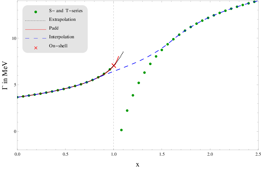
The asymptotic expansions and the three methods as well as the on-shell result are shown in Fig. 5. Fig. 6 contains the same curves on a larger scale plus curves for lower-order series up to 𝒪⁡(x8)\mathcal{O}(x^{8}) and 𝒪⁡(x9)\mathcal{O}(x^{9}) as well as their associated Padé approximants P(1)​[5,4]P^{(1)}[5,4] and P(1)​[4,4]P^{(1)}[4,4].44 4 Alternatively, P(1)​[4,5]P^{(1)}[4,5] may be used as Padé approximation for the series up to 𝒪⁡(x9)\mathcal{O}(x^{9}). For all diagrams, this approximant yields worse on-shell approximated values compared to its inverse P(1)​[5,4]P^{(1)}[5,4]. Consequently, we will use Padé approximations of the form P(1)​[n/2+1/2,n/2−1/2]P^{(1)}[n/2+1/2,n/2-1/2] whenever we have to apply them to series up to 𝒪⁡(xn)\mathcal{O}(x^{n}) with odd number nn. Although for this diagram the interpolation method seems to agree best with the exact on-shell result at NLO, at NNLO we will use the numerical value obtained by the Padé approximation for the following reasons:

  • •

    First, the Padé approximant is better suited than the extrapolation and interpolation methods for every other diagram and we would like to find a consistent method for all diagrams.

  • •

    Second and more important, we would like to avoid results depending on asymptotic expansions for x≫1x\gg 1 as far as possible. They still involve problems with respect to their convergence, which are associated with cuts of massive boson lines. Hence, the interpolation method will be only used as a cross check.

Let us proceed with diagram (g)(g). For this purpose, we introduce additional diagrams which originate from the field renormalization constant of the WW boson,

δ​ZW=−Re​∂∂q2​ΠTW​(MW2),\delta Z_{W}=-\mathrm{Re}\,\frac{\partial}{\partial q^{2}}\,\Pi^{W}_{T}(M_{W}^{2})\,, (25)

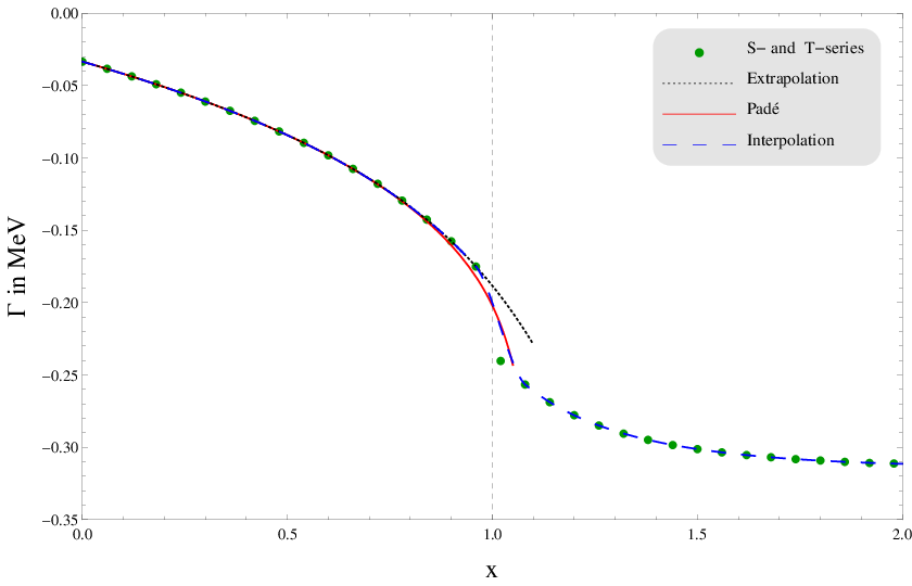
where ΠTW\Pi^{W}_{T} is the transversal part of the WW boson two-point function. The derivative with respect to q2q^{2} of its contributions with a photon inside the loop can be depicted via group (h)(h) in Fig. 9. In the following, only the sum of (g)(g) and (h)(h) will be considered. This is due to infrared (IR) divergences which occur solely in the on-shell computations of (g)(g) and (h)(h). Consequently, they do not match the off-shell calculations at all and the approximation methods cannot be applied. However, both the on- and the off-shell result of the combination (g)+(h)(g)+(h) is IR finite so that Figs. 7 and 8 provide a basis well suited for the determination of the NNLO result through a Padé approximated SS-series:

Pg+h(1)​[5,5]=−0.010​x5−0.085​x4+0.504​x3+0.092​x2−2.001​x+1.5731.04⋅10−3​x5+0.036​x4−0.459​x3+1.611​x2−2.174​x+1.P^{(1)}_{g+h}[5,5]=\frac{-0.010\,x^{5}-0.085\,x^{4}+0.504\,x^{3}+0.092\,x^{2}-2.001\,x+1.573}{1.04\cdot 10^{-3}\,x^{5}+0.036\,x^{4}-0.459\,x^{3}+1.611\,x^{2}-2.174\,x+1}\,. (26)
Refer to caption
Figure 5: NLO plot for diagram (f)\boldsymbol{(f)} including the SS-series, the TT-series, the extrapolation of the SS-series, the [5,5][5,5] Padé approximation of the SS-series, the interpolation of the SS- and TT-series and the exact on-shell result. Every series is plotted up to 𝒪⁡(x±10)\mathcal{O}(x^{\pm 10}).
Refer to caption
Figure 6: NLO plot for diagram (f)\boldsymbol{(f)} on a larger scale including the SS-series, the TT-series, the extrapolation of the SS-series, the Padé approximation of the SS-series, the interpolation of the SS- and TT-series and the exact on-shell result. The SS-series and the extrapolation (the TT-series and the interpolation on the right-hand side) are plotted up to 𝒪⁡(x±8)\mathcal{O}(x^{\pm 8}), 𝒪⁡(x±9)\mathcal{O}(x^{\pm 9}) and 𝒪⁡(x±10)\mathcal{O}(x^{\pm 10}) corresponding to the three curves from top to bottom (from bottom to top), respectively. The [4,4][4,4], [5,4][5,4] and [5,5][5,5] Padé approximations correspond to the three curves from top to bottom.
Refer to caption
Figure 7: Combined NLO plot for the diagrams (g)\boldsymbol{(g)} and (h)\boldsymbol{(h)} including the SS-series, the TT-series, the extrapolation of the SS-series, the [5,5][5,5] Padé approximation of the SS-series, the interpolation of the SS- and TT-series and the exact on-shell result. Every series is plotted up to 𝒪⁡(x±10)\mathcal{O}(x^{\pm 10}).
Refer to caption
Figure 8: Combined NLO plot for the diagrams (g)\boldsymbol{(g)} and (h)\boldsymbol{(h)} on a larger scale including the SS-series, the extrapolation of the SS-series, the Padé approximation of the SS-series, the interpolation of the SS- and TT-series and the exact on-shell result. The SS-series, the extrapolation and the interpolation are plotted up to 𝒪⁡(x±8)\mathcal{O}(x^{\pm 8}), 𝒪⁡(x±9)\mathcal{O}(x^{\pm 9}) and 𝒪⁡(x±10)\mathcal{O}(x^{\pm 10}) corresponding to the three curves from top to bottom, respectively. The [4,4][4,4], [5,4][5,4] and [5,5][5,5] Padé approximations correspond to the three curves from bottom to top.
Refer to caption
Figure 9: One-loop diagrams (h)\boldsymbol{(h)} for the calculation of the renormalization constant δ​ZW𝐃\boldsymbol{\delta Z^{\mathrm{D}}_{W}} designed to cancel the on-shell IR divergence of diagram (g)(g). Φ\Phi stands for charged Goldstone bosons whereas the dots on the lines indicate that the associated propagator appears twice as a consequence of the derivative with respect to q2q^{2}.

The individual contributions of group (g)(g) to the exact on-shell result and the tt-series are given by

Γg(1)\displaystyle\Gamma^{(1)}_{g} =Γ(0)​απ​(299+12​1ϵIR+ln​μ2MW2),\displaystyle=\Gamma^{(0)}\,\frac{\alpha}{\pi}\,\left(\frac{29}{9}+\frac{1}{2}\,\frac{1}{\epsilon_{\mathrm{IR}}}+\mathrm{ln}\,\frac{\mu^{2}}{M_{W}^{2}}\right)\,, (27)
tg(1)\displaystyle t^{(1)}_{g} =68972+1112​1ϵ+116​ln​μ2MW2−116​ln​x+(−16924−114​1ϵ−112​ln​μ2MW2+112​ln​x)​1x\displaystyle=\frac{689}{72}+\frac{11}{12}\,\frac{1}{\epsilon}+\frac{11}{6}\,\mathrm{ln}\,\frac{\mu^{2}}{M_{W}^{2}}-\frac{11}{6}\,\mathrm{ln}\,x+\left(-\frac{169}{24}-\frac{11}{4}\,\frac{1}{\epsilon}-\frac{11}{2}\,\mathrm{ln}\,\frac{\mu^{2}}{M_{W}^{2}}+\frac{11}{2}\,\mathrm{ln}\,x\right)\frac{1}{x}
+(−36172+56​1ϵ+53​ln​μ2MW2−53​ln​x)​1x2−1516​1x3−1920​1x4−3748​1x5−177288​1x6\displaystyle\,\quad+\left(-\frac{361}{72}+\frac{5}{6}\,\frac{1}{\epsilon}+\frac{5}{3}\,\mathrm{ln}\,\frac{\mu^{2}}{M_{W}^{2}}-\frac{5}{3}\,\mathrm{ln}\,x\right)\frac{1}{x^{2}}-\frac{15}{16}\frac{1}{x^{3}}-\frac{19}{20}\,\frac{1}{x^{4}}-\frac{37}{48}\,\frac{1}{x^{5}}-\frac{177}{288}\,\frac{1}{x^{6}}
−1732​1x7−115252​1x8−4471220​1x9−1748​1x10+𝒪⁡(1x11).\displaystyle\,\quad-\frac{17}{32}\,\frac{1}{x^{7}}-\frac{115}{252}\,\frac{1}{x^{8}}-\frac{447}{1220}\,\frac{1}{x^{9}}-\frac{17}{48}\,\frac{1}{x^{10}}+\mathcal{O}\left(\frac{1}{x^{11}}\right)\,. (28)

For group (h)(h), the individual contributions read as follows:

Γh(1)\displaystyle\Gamma^{(1)}_{h} =Γϵ(0)​απ​(13172+1924​1ϵ+1924​ln​μ2MW2+[−1−12​1ϵ−12​ln​μ2MW2]IR),\displaystyle=\Gamma^{(0)}_{\epsilon}\,\frac{\alpha}{\pi}\,\left(\frac{131}{72}+\frac{19}{24}\,\frac{1}{\epsilon}+\frac{19}{24}\,\mathrm{ln}\,\frac{\mu^{2}}{M_{W}^{2}}+\left[-1-\frac{1}{2}\,\frac{1}{\epsilon}-\frac{1}{2}\,\mathrm{ln}\,\frac{\mu^{2}}{M_{W}^{2}}\right]_{\mathrm{IR}}\right)\,, (29)
Sh(1)\displaystyle S^{(1)}_{h} =Γϵ(0)​απ​(143144+1924​1ϵ+4348​x+1532​x2+2372​x3+163672​x4+2191120​x5+2831728​x6CLOSE\displaystyle=\Gamma^{(0)}_{\epsilon}\,\frac{\alpha}{\pi}\,\left(\frac{143}{144}+\frac{19}{24}\,\frac{1}{\epsilon}+\frac{43}{48}\,x+\frac{15}{32}\,x^{2}+\frac{23}{72}\,x^{3}+\frac{163}{672}\,x^{4}+\frac{219}{1120}\,x^{5}\right.+\frac{283}{1728}\,x^{6}
OPEN+71504​x7+87704​x8+5234752​x9+6196240​x10)+𝒪⁡(x11),\displaystyle\qquad\qquad\quad\left.+\frac{71}{504}\,x^{7}+\frac{87}{704}\,x^{8}+\frac{523}{4752}\,x^{9}+\frac{619}{6240}\,x^{10}\right)+\mathcal{O}\left(x^{11}\right)\,, (30)
Th(1)\displaystyle T^{(1)}_{h} =Γϵ(0)​απ​(4336+1924​1ϵ+1924​ln​μ2MW2−1924​ln​x+(1316−58​ln​x)​1xCLOSE\displaystyle=\Gamma^{(0)}_{\epsilon}\,\frac{\alpha}{\pi}\,\left(\frac{43}{36}+\frac{19}{24}\,\frac{1}{\epsilon}+\frac{19}{24}\,\mathrm{ln}\,\frac{\mu^{2}}{M_{W}^{2}}-\frac{19}{24}\,\mathrm{ln}\,x+\left(\frac{13}{16}-\frac{5}{8}\,\mathrm{ln}\,x\right)\frac{1}{x}\right.
+(89+512​ln​x)​1x2+332​1x3+19120​1x4+43288​1x5+15112​1x6\displaystyle\qquad\qquad\quad+\left(\frac{8}{9}+\frac{5}{12}\,\mathrm{ln}\,x\right)\frac{1}{x^{2}}+\frac{3}{32}\,\frac{1}{x^{3}}+\frac{19}{120}\,\frac{1}{x^{4}}+\frac{43}{288}\,\frac{1}{x^{5}}+\frac{15}{112}\,\frac{1}{x^{6}}
OPEN+23192​1x7+1631512​1x8+2192240​1x9+2833168​1x10)+𝒪⁡(1x11).\displaystyle\qquad\qquad\quad\left.+\frac{23}{192}\,\frac{1}{x^{7}}+\frac{163}{1512}\,\frac{1}{x^{8}}+\frac{219}{2240}\,\frac{1}{x^{9}}+\frac{283}{3168}\,\frac{1}{x^{10}}\right)+\mathcal{O}\left(\frac{1}{x^{11}}\right)\,. (31)

The subscript IR refers to an IR pole in contrast to a UV one (without a subscript).
The total contribution to the electroweak corrections is then given by the sum

ΓEW(1)=Γconv(1)+Γslow(1)+Γren(1).\Gamma^{(1)}_{\mathrm{EW}}=\Gamma^{(1)}_{\mathrm{conv}}+\Gamma^{(1)}_{\mathrm{slow}}+\Gamma^{(1)}_{\mathrm{ren}}\,. (32)

Note that renormalization constants have to be multiplied by Γϵ(0)\Gamma^{(0)}_{\epsilon}, the Born width up to 𝒪⁡(ϵ)\mathcal{O}(\epsilon) in Eq. (6), instead of Γ(0)\Gamma^{(0)}. That way, an additional finite part is picked up from the multiplication of the pole part of the renormalization constant by the 𝒪⁡(ϵ)\mathcal{O}(\epsilon) term of the Born decay width. We have applied an on-shell renormalization scheme described in Ref. [47], leading to

Γren(1)=2​Γϵ(0)​δ​Z.\Gamma^{(1)}_{\mathrm{ren}}=2\,\Gamma^{(0)}_{\epsilon}\,\delta Z\,. (33)

From the renormalized charged current vertex, it follows that

δ​Z\displaystyle\delta Z ≡δ​Ze−δ​swsw+12​δ​ZW\displaystyle\equiv\delta Z_{e}-\frac{\delta s_{w}}{s_{w}}+\frac{1}{2}\,\delta Z_{W} (34)
=12​∂∂q2​ΠTγ​(0)−swcw​ΠTγ​Z​(0)MZ2+cw22​sw2​Re​(ΠTW​(MW2)MW2−ΠTZ​(MZ2)MZ2)−12​∂∂q2​ΠTW​(MW2).\displaystyle=\frac{1}{2}\,\frac{\partial}{\partial q^{2}}\,\Pi^{\gamma}_{T}(0)-\frac{s_{w}}{c_{w}}\,\frac{\Pi^{\gamma Z}_{T}(0)}{M_{Z}^{2}}+\frac{c_{w}^{2}}{2\,s_{w}^{2}}\,\mathrm{Re}\,\left(\frac{\Pi^{W}_{T}(M_{W}^{2})}{M_{W}^{2}}-\frac{\Pi^{Z}_{T}(M_{Z}^{2})}{M_{Z}^{2}}\right)-\frac{1}{2}\,\frac{\partial}{\partial q^{2}}\,\Pi^{W}_{T}(M_{W}^{2})\,.

At this point, we should comment on the parameterization of our calculations. All preceding formulae have used α\alpha and the physical particle masses as basic parameters. In such on-shell renormalization schemes, large electroweak corrections arise from fermion loop contributions to the renormalization of α\alpha and sws_{w}. As in any charged-current process, these corrections can be reduced by parameterizing the lowest-order result with Fermi’s coupling constant GFG_{F} and MWM_{W} instead [48]. This can be achieved with the help of the relationship

GF=π​α2​sw2​MW2​11−Δ​r.G_{F}=\frac{\pi\,\alpha}{\sqrt{2}\,s_{w}^{2}\,M_{W}^{2}}\frac{1}{1-\Delta r}\,. (35)

Δ​r\Delta r contains the radiative corrections to the muon decay width which the Standard Model introduces in addition to the purely photonic corrections from within Fermi’s model. At one loop, this expression is finite and given by [47, 48]

Δ​r\displaystyle\Delta r =ΠTW​(0)−Re​ΠTW​(MW2)MW2+cw2sw2​Re​(ΠTW​(MW2)MW2−ΠTZ​(MZ2)MZ2)+2​cwsw​ΠTγ​Z​(0)MZ2\displaystyle=\frac{\Pi^{W}_{T}(0)-\mathrm{Re}\,\Pi^{W}_{T}(M_{W}^{2})}{M_{W}^{2}}+\frac{c_{w}^{2}}{s_{w}^{2}}\,\mathrm{Re}\,\left(\frac{\Pi^{W}_{T}(M_{W}^{2})}{M_{W}^{2}}-\frac{\Pi^{Z}_{T}(M_{Z}^{2})}{M_{Z}^{2}}\right)+2\,\frac{c_{w}}{s_{w}}\,\frac{\Pi^{\gamma Z}_{T}(0)}{M_{Z}^{2}}
+∂∂q2​ΠTγ​(0)+α4​π​sw2​[(72​sw2−2)​ln​cw2+6].\displaystyle\,\quad+\frac{\partial}{\partial q^{2}}\,\Pi^{\gamma}_{T}(0)+\frac{\alpha}{4\,\pi\,s_{w}^{2}}\,\left[\left(\frac{7}{2\,s_{w}^{2}}-2\right)\,\mathrm{ln}\,c_{w}^{2}+6\right]\,. (36)

The term in the square brackets is obtained by the vertex and box corrections to the muon decay width in Feynman-’t Hooft gauge. Hence, the self-energies ΠT\Pi_{T} have to be calculated in the same gauge. This requires the computation of

∂∂q2​ΠTγ​(0),\frac{\partial}{\partial q^{2}}\,\Pi^{\gamma}_{T}(0)\,, (37)

which receives important contributions from the light quark flavors. They cannot be reliably predicted in perturbative QCD so that the gauge-independent and finite quantity

Δ​αhad(5)=[∂∂q2​ΠTγ​(0)−ΠTγ​(MZ2)MZ2]u​d​s​c​b\Delta\alpha^{(5)}_{\mathrm{had}}=\left[\frac{\partial}{\partial q^{2}}\,\Pi^{\gamma}_{T}(0)-\frac{\Pi^{\gamma}_{T}(M_{Z}^{2})}{M_{Z}^{2}}\right]_{udscb} (38)

is introduced. That way, experimental data on the total cross section of inclusive hadron production in e+​e−e^{+}e^{-} annihilation can be used to circumvent the problem. However, we substitute

α=2​GF​sw2​MW2π\alpha=\frac{\sqrt{2}\,G_{F}\,s_{w}^{2}\,M_{W}^{2}}{\pi} (39)

whenever the lowest-order result Γ(0)\Gamma^{(0)} of Eq. (5) appears within our calculations. In turn, we add the term −Γ(0)ϵ⋅Δr-\Gamma^{(0)}_{\epsilon}\cdot\Delta r to Eq. (33) so that the quantity ∂/∂q2​ΠTγ​(0)\partial/\partial q^{2}\,\Pi^{\gamma}_{T}(0) exactly cancels and the theoretical uncertainty of Δ​αhad(5)\Delta\alpha^{(5)}_{\mathrm{had}} does not affect our results:

Γren(1)=Γϵ(0)​(2​δ​Z−Δ​r).\Gamma^{(1)}_{\mathrm{ren}}=\Gamma^{(0)}_{\epsilon}\,\left(2\,\delta Z-\Delta r\right)\,. (40)

The pole part of Γren(1)\Gamma^{(1)}_{\mathrm{ren}} in Eq. (32) is then given by

Γ~ren(1)=−Γ(0)​απ​(1sw2​ϵ+12​1ϵIR)=−(Γ~conv(1)+Γ~slow(1)).\tilde{\Gamma}^{(1)}_{\mathrm{ren}}=-\Gamma^{(0)}\,\frac{\alpha}{\pi}\,\left(\frac{1}{s_{w}^{2}\,\epsilon}+\frac{1}{2}\,\frac{1}{\epsilon_{\mathrm{IR}}}\right)=-\left(\tilde{\Gamma}^{(1)}_{\mathrm{conv}}+\tilde{\Gamma}^{(1)}_{\mathrm{slow}}\right)\,. (41)

Hence, the renormalization procedure cancels both the UV and the on-shell IR divergences and thus produces a physical quantity.

2.3 Next-To-Next-To-Leading-Order Decay Width:
Mixed QCD/Electroweak Corrections of Order 𝜶​𝜶𝒔\boldsymbol{\alpha\,\alpha_{s}}

The calculation of the mixed QCD/electroweak corrections follows the same logic as the computation of the electroweak corrections in Section 2.2:

Γmixed(2)=Γconv(2)+Γslow(2)+Γren(2).\Gamma^{(2)}_{\mathrm{mixed}}=\Gamma^{(2)}_{\mathrm{conv}}+\Gamma^{(2)}_{\mathrm{slow}}+\Gamma^{(2)}_{\mathrm{ren}}\,. (42)

All diagrams in question can be obtained by adding exactly one gluon to the NLO electroweak diagrams in every possible way. Thus, we can reuse the labeling of the diagrams in Fig. 4, which is depicted in Fig. 10.

Refer to caption
Refer to caption
Figure 10: Three-loop diagrams for the calculation of the 𝒪⁡(α​αs)\boldsymbol{\mathcal{O}(\alpha\,\alpha_{s})} mixed QCD/ electroweak corrections Γmixed(2)\Gamma^{(2)}_{\mathrm{mixed}}. The labeling corresponds to the seven groups (a)−(g)(a)-(g) of Fig. 4. By adding one gluon in every possible way, these eighteen topologies occur. The straight lines stand for quarks, the curly lines for gluons and the wavy ones denote photons, ZZ or WW bosons.

As a first step, the convergent diagrams have to be separated from the slowly converging ones by applying the hard mass procedure. This yields a result of the form

S(2)=Γ(0)​απ​αsπ​∑n=0∞dn​xn≡Γ(0)​απ​αsπ​s(2),S^{(2)}=\Gamma^{(0)}\,\frac{\alpha}{\pi}\,\frac{\alpha_{s}}{\pi}\,\sum_{n=0}^{\infty}d_{n}\,x^{n}\equiv\Gamma^{(0)}\,\frac{\alpha}{\pi}\,\frac{\alpha_{s}}{\pi}\,s^{(2)}\,, (43)

where we have made use of the relationship

nc2=2​nc​CF+1n_{c}^{2}=2\,n_{c}\,C_{F}+1 (44)

in order to factor out the Born decay width Γ(0)\Gamma^{(0)}. CFC_{F} is the quadratic Casimir operator of the fundamental representation S​U​(nc)SU(n_{c}) of the strong interaction. For three colors, it is given by CF=4/3C_{F}=\nicefrac{{4}}{{3}}.
We computed the coefficients dnd_{n} for every group (a)−(g)(a)-(g) up to 𝒪⁡(x9)\mathcal{O}(x^{9}):

sa(2)\displaystyle s^{(2)}_{a} =sa​1(2)+sa​2(2)=−433144+2​ζ​(3)−18​1ϵ−38​ln​μ2MW2+38​ln​x,\displaystyle=s^{(2)}_{a1}+s^{(2)}_{a2}=-\frac{433}{144}+2\,\zeta(3)-\frac{1}{8}\,\frac{1}{\epsilon}-\frac{3}{8}\,\mathrm{ln}\,\frac{\mu^{2}}{M_{W}^{2}}+\frac{3}{8}\,\mathrm{ln}\,x\,,
sb(2)\displaystyle s^{(2)}_{b} =cwsw(gq−gq′)[1038−12ζ(3)+541ϵ+154lnμ2MW2−114lnx−718x−892160x2\displaystyle=\frac{c_{w}}{s_{w}}\left(g_{q}-g_{q^{\prime}}\right)\left[\frac{103}{8}-12\,\zeta(3)+\frac{5}{4}\,\frac{1}{\epsilon}+\frac{15}{4}\,\mathrm{ln}\,\frac{\mu^{2}}{M_{W}^{2}}-\frac{11}{4}\,\mathrm{ln}\,x-\frac{7}{18}\,x-\frac{89}{2160}\,x^{2}\right.
−294725​x3−5350400​x4−8514365900​x5−138136324288​x6−34945405360​x7\displaystyle\qquad\qquad\qquad\qquad-\frac{29}{4725}\,x^{3}-\frac{53}{50400}\,x^{4}-\frac{851}{4365900}\,x^{5}-\frac{1381}{36324288}\,x^{6}-\frac{349}{45405360}\,x^{7}
−30171890345600x8−417712346319700x9]+𝒪(x10),\displaystyle\qquad\qquad\qquad\qquad\left.-\frac{3017}{1890345600}\,x^{8}-\frac{4177}{12346319700}\,x^{9}\right]+\mathcal{O}\left(x^{10}\right)\,,
sc(2)\displaystyle s^{(2)}_{c} =1sw2[(−8948+2ζ(3)−181ϵ−38lnμ2MW2+38lnx)+(−121243+2281lnx−127ln2x)x\displaystyle=\frac{1}{s_{w}^{2}}\,\left[\left(-\frac{89}{48}+2\,\zeta(3)-\frac{1}{8}\,\frac{1}{\epsilon}-\frac{3}{8}\,\mathrm{ln}\,\frac{\mu^{2}}{M_{W}^{2}}+\frac{3}{8}\,\mathrm{ln}\,x\right)+\left(-\frac{121}{243}+\frac{22}{81}\,\mathrm{ln}\,x-\frac{1}{27}\,\mathrm{ln}^{2}\,x\right)x\right.
+(−16915552+131296​ln​x−1432​ln2​x)​x2\displaystyle\quad\qquad+\left(-\frac{169}{15552}+\frac{13}{1296}\,\mathrm{ln}\,x-\frac{1}{432}\,\mathrm{ln}^{2}\,x\right)x^{2}
+(−22092430000+4740500​ln​x−12700​ln2​x)​x3\displaystyle\quad\qquad+\left(-\frac{2209}{2430000}+\frac{47}{40500}\,\mathrm{ln}\,x-\frac{1}{2700}\,\mathrm{ln}^{2}\,x\right)x^{3}
+(−13699720000+37162000​ln​x−110800​ln2​x)​x4\displaystyle\quad\qquad+\left(-\frac{1369}{9720000}+\frac{37}{162000}\,\mathrm{ln}\,x-\frac{1}{10800}\,\mathrm{ln}^{2}\,x\right)x^{4}
+(−11449364651875+2143472875​ln​x−133075​ln2​x)​x5\displaystyle\quad\qquad+\left(-\frac{11449}{364651875}+\frac{214}{3472875}\,\mathrm{ln}\,x-\frac{1}{33075}\,\mathrm{ln}^{2}\,x\right)x^{5}
+(−5329597445632+733556224​ln​x−184672​ln2​x)​x6\displaystyle\quad\qquad+\left(-\frac{5329}{597445632}+\frac{73}{3556224}\,\mathrm{ln}\,x-\frac{1}{84672}\,\mathrm{ln}^{2}\,x\right)x^{6}
+(−3648112098274048+19124004512​ln​x−1190512​ln2​x)​x7\displaystyle\quad\qquad+\left(-\frac{36481}{12098274048}+\frac{191}{24004512}\,\mathrm{ln}\,x-\frac{1}{190512}\,\mathrm{ln}^{2}\,x\right)x^{7}
+(−1464112597120000+12134992000​ln​x−1388800​ln2​x)​x8\displaystyle\quad\qquad+\left(-\frac{14641}{12597120000}+\frac{121}{34992000}\,\mathrm{ln}\,x-\frac{1}{388800}\,\mathrm{ln}^{2}\,x\right)x^{8}
+(−89401180111751875+598363862125lnx−1735075ln2x)x9]+𝒪(x10),\displaystyle\quad\qquad\left.+\left(-\frac{89401}{180111751875}+\frac{598}{363862125}\,\mathrm{ln}\,x-\frac{1}{735075}\,\mathrm{ln}^{2}\,x\right)x^{9}\right]+\mathcal{O}\left(x^{10}\right)\,,
sd(2)\displaystyle s^{(2)}_{d} =(gq2+gq′2)​sw2​sc(2),\displaystyle=\left(g_{q}^{2}+g_{q^{\prime}}^{2}\right)\,s_{w}^{2}\,s^{(2)}_{c}\,, (45)
se(2)\displaystyle s^{(2)}_{e} =gqgq′[(8924−4ζ(3)+141ϵ+34lnμ2MW2−34lnx)\displaystyle=g_{q}\,g_{q^{\prime}}\left[\left(\frac{89}{24}-4\,\zeta(3)+\frac{1}{4}\,\frac{1}{\epsilon}+\frac{3}{4}\,\mathrm{ln}\,\frac{\mu^{2}}{M_{W}^{2}}-\frac{3}{4}\,\mathrm{ln}\,x\right)\right.
+(7127−43​ζ​(3)−23​ln​x−13​ln2​x)​x\displaystyle\qquad\qquad+\left(\frac{71}{27}-\frac{4}{3}\,\zeta(3)-\frac{2}{3}\,\mathrm{ln}\,x-\frac{1}{3}\,\mathrm{ln}^{2}\,x\right)x
+(−11592592+13​ζ​(3)+56​ln​x−736​ln2​x)​x2\displaystyle\qquad\qquad+\left(-\frac{1159}{2592}+\frac{1}{3}\,\zeta(3)+\frac{5}{6}\,\mathrm{ln}\,x-\frac{7}{36}\,\mathrm{ln}^{2}\,x\right)x^{2}
+(−185310800−215​ζ​(3)−1390​ln​x)​x3\displaystyle\qquad\qquad+\left(-\frac{1853}{10800}-\frac{2}{15}\,\zeta(3)-\frac{13}{90}\,\mathrm{ln}\,x\right)x^{3}
+(146179972000+115​ζ​(3)+83810​ln​x−11180​ln2​x)​x4\displaystyle\qquad\qquad+\left(\frac{146179}{972000}+\frac{1}{15}\,\zeta(3)+\frac{83}{810}\,\mathrm{ln}\,x-\frac{11}{180}\,\mathrm{ln}^{2}\,x\right)x^{4}
+(−78941595350−4105​ζ​(3)−372835​ln​x)​x5\displaystyle\qquad\qquad+\left(-\frac{78941}{595350}-\frac{4}{105}\,\zeta(3)-\frac{37}{2835}\,\mathrm{ln}\,x\right)x^{5}
+(5143284975334336000+142​ζ​(3)+22112960​ln​x−1435040​ln2​x)​x6\displaystyle\qquad\qquad+\left(\frac{514328497}{5334336000}+\frac{1}{42}\,\zeta(3)+\frac{221}{12960}\,\mathrm{ln}\,x-\frac{143}{5040}\,\mathrm{ln}^{2}\,x\right)x^{6}
+(−2627584133429216000−163​ζ​(3)+799136080​ln​x−11080​ln2​x)​x7\displaystyle\qquad\qquad+\left(-\frac{262758413}{3429216000}-\frac{1}{63}\,\zeta(3)+\frac{799}{136080}\,\mathrm{ln}\,x-\frac{1}{1080}\,\mathrm{ln}^{2}\,x\right)x^{7}
+(13907067061240045120000+190​ζ​(3)+8536804000​ln​x−40325200​ln2​x)​x8\displaystyle\qquad\qquad+\left(\frac{13907067061}{240045120000}+\frac{1}{90}\,\zeta(3)+\frac{853}{6804000}\,\mathrm{ln}\,x-\frac{403}{25200}\,\mathrm{ln}^{2}\,x\right)x^{8}
+(−42384988309907670610000−4495ζ(3)+190582338875lnx−119450ln2x)x9]+𝒪(x10),\displaystyle\qquad\qquad\left.+\left(-\frac{42384988309}{907670610000}-\frac{4}{495}\,\zeta(3)+\frac{19058}{2338875}\,\mathrm{ln}\,x-\frac{11}{9450}\,\mathrm{ln}^{2}\,x\right)x^{9}\right]+\mathcal{O}\left(x^{10}\right)\,,
sf(2)\displaystyle s^{(2)}_{f} =1118+54​1ϵ−12​ζ​(3)+154​ln​μ2MW2−114​ln​x+(−1157864+59​ln​x)​x\displaystyle=\frac{111}{8}+\frac{5}{4}\,\frac{1}{\epsilon}-12\,\zeta(3)+\frac{15}{4}\,\mathrm{ln}\,\frac{\mu^{2}}{M_{W}^{2}}-\frac{11}{4}\,\mathrm{ln}\,x+\left(-\frac{1157}{864}+\frac{5}{9}\,\mathrm{ln}\,x\right)x
+(−20714320+2572​ln​x)​x2+(−542321600+2390​ln​x)​x3+(−23459151200+73360​ln​x)​x4\displaystyle\,\quad+\left(-\frac{2071}{4320}+\frac{25}{72}\,\mathrm{ln}\,x\right)x^{2}+\left(-\frac{5423}{21600}+\frac{23}{90}\,\mathrm{ln}\,x\right)x^{3}+\left(-\frac{23459}{151200}+\frac{73}{360}\,\mathrm{ln}\,x\right)x^{4}
+(−2233992116800+53315​ln​x)​x5+(−161921168+1451008​ln​x)​x6\displaystyle\,\quad+\left(-\frac{223399}{2116800}+\frac{53}{315}\,\mathrm{ln}\,x\right)x^{5}+\left(-\frac{1619}{21168}+\frac{145}{1008}\,\mathrm{ln}\,x\right)x^{6}
+(−2209613810240+95756​ln​x)​x7+(−8843194400+2412160​ln​x)​x8\displaystyle\,\quad+\left(-\frac{220961}{3810240}+\frac{95}{756}\,\mathrm{ln}\,x\right)x^{7}+\left(-\frac{8843}{194400}+\frac{241}{2160}\,\mathrm{ln}\,x\right)x^{8}
+(−86182723522400+1491485​ln​x)​x9+𝒪⁡(x10),\displaystyle\,\quad+\left(-\frac{861827}{23522400}+\frac{149}{1485}\,\mathrm{ln}\,x\right)x^{9}+\mathcal{O}\left(x^{10}\right)\,,
sg(2)\displaystyle s^{(2)}_{g} =−116​x2−19180​x3−37336​x4−59560​x5−85864​x6−23252​x7−1491760​x8−17216​x9\displaystyle=-\frac{1}{16}\,x^{2}-\frac{19}{180}\,x^{3}-\frac{37}{336}\,x^{4}-\frac{59}{560}\,x^{5}-\frac{85}{864}\,x^{6}-\frac{23}{252}\,x^{7}-\frac{149}{1760}\,x^{8}-\frac{17}{216}\,x^{9}
+𝒪⁡(x10).\displaystyle\,\quad+\mathcal{O}\left(x^{10}\right)\,. (45)

The asymptotic series of the entire NNLO contribution is given by the sum of these expressions:

S(2)=∑i=agSi(2).S^{(2)}=\sum_{i=a}^{g}S^{(2)}_{i}\,. (46)

As in case of the NLO electroweak analog (Eqs. (12)), Eqs. (45) do not indicate the general result, but for the special case MZ=MWM_{Z}=M_{W}. Again, we account for the mass difference of the WW and the ZZ boson by performing a Taylor expansion in the exact same manner as in Section 2.2. In doing so, we pick up additional expressions of the form

Γ(0)​απ​αsπ​∑n=08∑m=1min⁡(5,9−n)bn,m​xn​δm\Gamma^{(0)}\,\frac{\alpha}{\pi}\,\frac{\alpha_{s}}{\pi}\,\sum_{n=0}^{8}\,\sum_{m=1}^{\mathrm{min}(5,9-n)}b_{n,m}\,x^{n}\,\delta^{m} (47)

with

δ=MW2−MZ2MW2=−sw2cw2≈−0.29\delta=\frac{M_{W}^{2}-M_{Z}^{2}}{M_{W}^{2}}=-\frac{s_{w}^{2}}{c_{w}^{2}}\approx-0.29 (16)

within the SS-series of every group involving a ZZ boson. The coefficients bn,mb_{n,m} can be found in Appendix A.2. The upper bound of the second summation is given by the smaller number of 55 and 9−n9-n, which is denoted by the function ‘min\mathrm{min}’. This is due to Section 2.2, where we have decided that a Taylor expansion up to 𝒪⁡(δ5)\mathcal{O}(\delta^{5}) should be sufficient at NNLO because of the excellent convergence behavior of the Taylor expansion at NLO.
By adding the δm\delta^{m}-terms to the SS-series of the entire NNLO contribution for vanishing δ\delta (S(2)S^{(2)} in Eq. (46)), we obtain Sδ(2)S^{(2)}_{\delta}, which is the SS-series including δ\delta. Sδ(2)S^{(2)}_{\delta} can be used to study the convergence of the Taylor expansion by examining the difference of the SS-series including powers up to δp+1\delta^{p+1} and δp\delta^{p} for increasing pp:

Δp​Sδ(2)\displaystyle\Delta_{p}S^{(2)}_{\delta} ≡Γ(0)​απ​αsπ​∑n=08xn​(∑m=1pbn,m​δm−∑m=1p−1bn,m​δm)\displaystyle\equiv\Gamma^{(0)}\,\frac{\alpha}{\pi}\,\frac{\alpha_{s}}{\pi}\,\sum_{n=0}^{8}\,x^{n}\,\left(\sum_{m=1}^{p}b_{n,m}\,\delta^{m}-\sum_{m=1}^{p-1}b_{n,m}\,\delta^{m}\right)
=Γ(0)απαsπ∑n=08xnbn,pδp(p=2..5).\displaystyle=\Gamma^{(0)}\,\frac{\alpha}{\pi}\,\frac{\alpha_{s}}{\pi}\,\sum_{n=0}^{8}\,x^{n}\,b_{n,p}\,\delta^{p}\hskip 113.81102pt(p=2..5)\,. (48)
Table 3: Convergence of the Taylor expansion in δ\boldsymbol{\delta} for the entire NNLO contribution expressed through Δp​Sδ(2)\Delta_{p}S^{(2)}_{\delta} as defined in Eq. (48). All quantities are indicated for |Vq​q′|2=1\left|V_{qq^{\prime}}\right|^{2}=1. The numerical values are given in keV and the input parameters can be found in Section 3.
Δ2​Sδ(2)\Delta_{2}S^{(2)}_{\delta} +2.8+2.8
Δ3​Sδ(2)\Delta_{3}S^{(2)}_{\delta} +5.3+5.3
Δ4​Sδ(2)\Delta_{4}S^{(2)}_{\delta} +2.5+2.5
Δ5​Sδ(2)\Delta_{5}S^{(2)}_{\delta} +1.0+1.0
Sδ(2)S^{(2)}_{\delta} −642.0-642.0

We have calculated the coefficients up to 𝒪⁡(δ5)\mathcal{O}(\delta^{5}) so that a statement about the convergence can be made with the help of Table 3. From there, we can deduce that the Taylor series in the mass difference of the two bosons at NNLO converges sufficiently fast within the accuracy of the final result.
We use the results in Eqs. (45) to study the convergence of the asymptotic expansion by examining the difference of the SS-series including powers up to xj+1x^{j+1} and xjx^{j} for increasing jj. Again, this has been done for δ=0\delta=0 since the Taylor expansion in δ\delta has proven to converge:

Δj​S(2)\displaystyle\Delta_{j}S^{(2)} ≡Γ(0)​απ​αsπ​(∑n=0jdn​xn−∑n=0j−1dn​xn)\displaystyle\equiv\Gamma^{(0)}\,\frac{\alpha}{\pi}\,\frac{\alpha_{s}}{\pi}\,\left(\sum_{n=0}^{j}d_{n}\,x^{n}-\sum_{n=0}^{j-1}d_{n}\,x^{n}\right)
=Γ(0)απαsπdjxj(j=1..9).\displaystyle=\Gamma^{(0)}\,\frac{\alpha}{\pi}\,\frac{\alpha_{s}}{\pi}\,d_{j}\,x^{j}\hskip 113.81102pt(j=1..9)\,. (49)

The convergent diagrams can be separated from the slowly converging ones by means of Table 4, which shows the values of Δj​S(2)\Delta_{j}S^{(2)} for each group (a)−(g)(a)-(g). As at NLO, the groups (a)−(d)(a)-(d) belong to the convergent ones whereas (f)(f) and (g)(g) converge extremely slowly. However, the coefficients Δj​S(2)\Delta_{j}S^{(2)} for diagram (e)(e) lie in the same range as the values for (f)(f) and (g)(g) so that it will be counted amongst the slowly converging diagrams in contrast to the NLO calculation.

Table 4: Convergence of the asymptotic expansion in x\boldsymbol{x} for the various NNLO contributions expressed through Δj​S(2)\Delta_{j}S^{(2)} as defined in Eq. (49) for each group (a)−(g)(a)-(g) and their sum ∑\sum. All quantities are indicated for |Vq​q′|2=1\left|V_{qq^{\prime}}\right|^{2}=1. The numerical values are given in keV and the input parameters can be found in Section 3.
(a)(a) (b)(b) (c)(c) (d)(d) (e)(e) (f)(f) (g)(g) ∑\sum
Δ2​S(2)\Delta_{2}S^{(2)} 00 −8.7-8.7 −3.0-3.0 −1.2-1.2 +2.4+2.4 −29.1-29.1 −3.8-3.8 −43.4-43.4
Δ3​S(2)\Delta_{3}S^{(2)} 00 −1.3-1.3 −0.2-0.2 −9.7⋅10−2-9.7\cdot 10^{-2} +17.4+17.4 −15.3-15.3 −6.4-6.4 −5.9-5.9
Δ4​S(2)\Delta_{4}S^{(2)} 00 −0.2-0.2 −3.8⋅10−2-3.8\cdot 10^{-2} −1.5⋅10−2-1.5\cdot 10^{-2} −12.1-12.1 −9.4-9.4 −6.7-6.7 −28.6-28.6
Δ5​S(2)\Delta_{5}S^{(2)} 00 −4.1⋅10−2-4.1\cdot 10^{-2} −8.6⋅10−3-8.6\cdot 10^{-3} −3.4⋅10−3-3.4\cdot 10^{-3} +9.4+9.4 −6.4-6.4 −6.4-6.4 −3.5-3.5
Δ6​S(2)\Delta_{6}S^{(2)} 00 −8.1⋅10−3-8.1\cdot 10^{-3} −2.4⋅10−3-2.4\cdot 10^{-3} −9.5⋅10−4-9.5\cdot 10^{-4} −6.6-6.6 −4.6-4.6 −6.0-6.0 −17.2-17.2
Δ7​S(2)\Delta_{7}S^{(2)} 00 −1.6⋅10−3-1.6\cdot 10^{-3} −8.2⋅10−4-8.2\cdot 10^{-4} −3.2⋅10−4-3.2\cdot 10^{-4} +5.0+5.0 −3.5-3.5 −5.5-5.5 −4.1-4.1
Δ8​S(2)\Delta_{8}S^{(2)} 00 −3.3⋅10−4-3.3\cdot 10^{-4} −3.2⋅10−4-3.2\cdot 10^{-4} −1.2⋅10−4-1.2\cdot 10^{-4} −3.7-3.7 −2.8-2.8 −5.1-5.1 −11.7-11.7
Δ9​S(2)\Delta_{9}S^{(2)} 00 −7.2⋅10−5-7.2\cdot 10^{-5} −1.4⋅10−4-1.4\cdot 10^{-4} −5.3⋅10−5-5.3\cdot 10^{-5} +3.0+3.0 −2.2-2.2 −4.8-4.8 −4.1-4.1
S(2)S^{(2)} −36.6-36.6 −421.2-421.2 10.910.9 4.34.3 18.618.6 −188.3-188.3 −44.8-44.8 −657.0-657.0

Accordingly, the convergent diagrams’ contribution to the mixed QCD/electroweak corrections is given by the sum of the SS-series of the groups (a)−(d)(a)-(d):

Γconv(2)=∑i=adΓi(1)=limx→1∑i=adSi(2).\Gamma^{(2)}_{\mathrm{conv}}=\sum_{i=a}^{d}\Gamma^{(1)}_{i}=\lim_{x\to 1}\,\sum_{i=a}^{d}S^{(2)}_{i}\,. (50)

The contribution of the slowly converging diagrams to the mixed QCD/electroweak corrections stems from three parts corresponding to the groups (e)(e), (f)(f) and (g)(g):

Γslow(2)=Γe(2)+Γf(2)+Γg(2).\Gamma^{(2)}_{\mathrm{slow}}=\Gamma^{(2)}_{e}+\Gamma^{(2)}_{f}+\Gamma^{(2)}_{g}\,. (51)

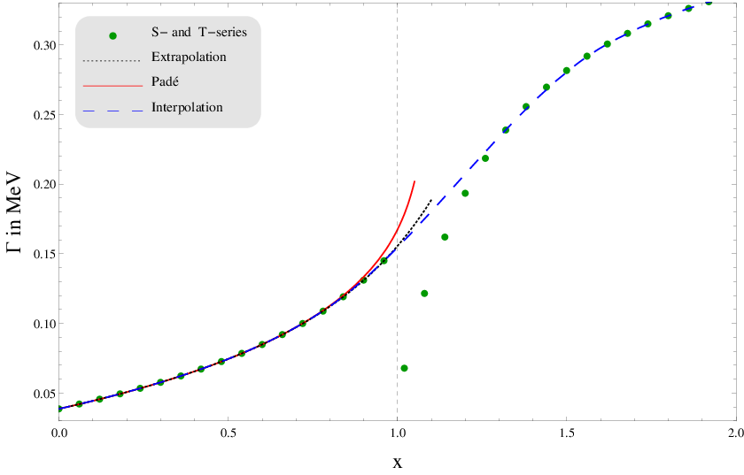
The determination of Γf(2)\Gamma^{(2)}_{f} and Γg(2)\Gamma^{(2)}_{g} is based on the approximation methods described in Section 2.2, whose prescriptions have been developed with the help of the NLO on-shell results. These prescriptions have been applied to the NNLO calculation, which results in Figs. 11 - 14. Besides the SS-series, we have computed the Padé approximant of the SS-series as well as the TT-series in order to obtain them:

Pf(2)​[5,4]\displaystyle P^{(2)}_{f}[5,4] =−1.37⋅10−4x5+9.11⋅10−3x4−0.056x3+0.090x2−0.014x−0.0330.026​x4−0.349​x3+1.371​x2−2.025​x+1,\displaystyle=\frac{-1.37\cdot 10^{-4}\,x^{5}+9.11\cdot 10^{-3}\,x^{4}-0.056\,x^{3}+0.090\,x^{2}-0.014\,x-0.033}{0.026\,x^{4}-0.349\,x^{3}+1.371\,x^{2}-2.025\,x+1}\,, (52)
tf(2)\displaystyle t^{(2)}_{f} =7724−203​ζ​(3)+712​1ϵ+74​ln​μ2MW2−174​ln​x\displaystyle=\frac{77}{24}-\frac{20}{3}\,\zeta(3)+\frac{7}{12}\,\frac{1}{\epsilon}+\frac{7}{4}\,\mathrm{ln}\,\frac{\mu^{2}}{M_{W}^{2}}-\frac{17}{4}\,\mathrm{ln}\,x
+(32548−7​ζ​(3)+78​1ϵ+218​ln​μ2MW2−5​ln​x)​1x\displaystyle\,\quad+\left(\frac{325}{48}-7\,\zeta(3)+\frac{7}{8}\,\frac{1}{\epsilon}+\frac{21}{8}\,\mathrm{ln}\,\frac{\mu^{2}}{M_{W}^{2}}-5\,\mathrm{ln}\,x\right)\frac{1}{x}
+(−61432+53​ζ​(3)−524​1ϵ−58​ln​μ2MW2+136​ln​x)​1x2+(151864−2572​ln​x)​1x3\displaystyle\,\quad+\left(-\frac{61}{432}+\frac{5}{3}\,\zeta(3)-\frac{5}{24}\,\frac{1}{\epsilon}-\frac{5}{8}\,\mathrm{ln}\,\frac{\mu^{2}}{M_{W}^{2}}+\frac{1}{36}\,\mathrm{ln}\,x\right)\frac{1}{x^{2}}+\left(\frac{151}{864}-\frac{25}{72}\,\mathrm{ln}\,x\right)\frac{1}{x^{3}}
+(381721600−2390​ln​x)​1x4+(277321600−73360​ln​x)​1x5\displaystyle\,\quad+\left(\frac{3817}{21600}-\frac{23}{90}\,\mathrm{ln}\,x\right)\frac{1}{x^{4}}+\left(\frac{2773}{21600}-\frac{73}{360}\,\mathrm{ln}\,x\right)\frac{1}{x^{5}} (53)
+(998231058400−53315​ln​x)​1x6+(15149211680−1451008​ln​x)​1x7\displaystyle\,\quad+\left(\frac{99823}{1058400}-\frac{53}{315}\,\mathrm{ln}\,x\right)\frac{1}{x^{6}}+\left(\frac{15149}{211680}-\frac{145}{1008}\,\mathrm{ln}\,x\right)\frac{1}{x^{7}}
+(42647762048−95756​ln​x)​1x8+(15271340200−2412160​ln​x)​1x9+𝒪⁡(1x10),\displaystyle\,\quad+\left(\frac{42647}{762048}-\frac{95}{756}\,\mathrm{ln}\,x\right)\frac{1}{x^{8}}+\left(\frac{15271}{340200}-\frac{241}{2160}\,\mathrm{ln}\,x\right)\frac{1}{x^{9}}+\mathcal{O}\left(\frac{1}{x^{10}}\right)\,, (53)
tg(2)\displaystyle t^{(2)}_{g} =15916−113​ζ​(3)+1124​1ϵ+118​ln​μ2MW2−118​ln​x\displaystyle=\frac{159}{16}-\frac{11}{3}\,\zeta(3)+\frac{11}{24}\,\frac{1}{\epsilon}+\frac{11}{8}\,\mathrm{ln}\,\frac{\mu^{2}}{M_{W}^{2}}-\frac{11}{8}\,\mathrm{ln}\,x
+(−21716+11​ζ​(3)−118​1ϵ−338​ln​μ2MW2+338​ln​x)​1x\displaystyle\,\quad+\left(-\frac{217}{16}+11\,\zeta(3)-\frac{11}{8}\,\frac{1}{\epsilon}-\frac{33}{8}\,\mathrm{ln}\,\frac{\mu^{2}}{M_{W}^{2}}+\frac{33}{8}\,\mathrm{ln}\,x\right)\frac{1}{x}
+(−1724−103​ζ​(3)+512​1ϵ+54​ln​μ2MW2−54​ln​x)​1x2−58​1x3−1930​1x4\displaystyle\,\quad+\left(-\frac{17}{24}-\frac{10}{3}\,\zeta(3)+\frac{5}{12}\,\frac{1}{\epsilon}+\frac{5}{4}\,\mathrm{ln}\,\frac{\mu^{2}}{M_{W}^{2}}-\frac{5}{4}\,\mathrm{ln}\,x\right)\frac{1}{x^{2}}-\frac{5}{8}\frac{1}{x^{3}}-\frac{19}{30}\,\frac{1}{x^{4}}
−3772​1x5−59140​1x6−1748​1x7−115378​1x8−149560​1x9+𝒪⁡(1x10).\displaystyle\,\quad-\frac{37}{72}\,\frac{1}{x^{5}}-\frac{59}{140}\,\frac{1}{x^{6}}-\frac{17}{48}\,\frac{1}{x^{7}}-\frac{115}{378}\,\frac{1}{x^{8}}-\frac{149}{560}\,\frac{1}{x^{9}}+\mathcal{O}\left(\frac{1}{x^{10}}\right)\,. (54)

As for the SS- and ss-series, we have introduced the abbreviated form of the inverse asymptotic expansion:

T(2)=Γ(0)​απ​αsπ​∑n=0∞d~nxn≡Γ(0)​απ​αsπ​t(2).T^{(2)}=\Gamma^{(0)}\,\frac{\alpha}{\pi}\,\frac{\alpha_{s}}{\pi}\,\sum_{n=0}^{\infty}\frac{\tilde{d}_{n}}{x^{n}}\equiv\Gamma^{(0)}\,\frac{\alpha}{\pi}\,\frac{\alpha_{s}}{\pi}\,t^{(2)}\,. (55)

According to Section 2.2, we have to combine group (g)(g) with the photonic contribution to the field renormalization constant δ​ZW\delta Z_{W} of the WW boson (Fig. 9). For this purpose, the SS- and TT-series of group (h)(h) have to be evaluated at NNLO. They immediately follow from the NLO expressions (Eqs. (30) and (31)) by multiplying the coefficients of the asymptotic expansion by the NLO QCD corrected width up to 𝒪⁡(ϵ)\mathcal{O}(\epsilon) (Eq. (9)) instead of the Born width up to 𝒪⁡(ϵ)\mathcal{O}(\epsilon) (Eq. (6)). Similarly, the on-shell result of (h)(h) at NNLO can be derived from Eq. (29):

Γh(2)\displaystyle\Gamma^{(2)}_{h} =ΓQCD,ϵ(1)Γϵ(0)​Γh(1),\displaystyle=\frac{\Gamma^{(1)}_{\mathrm{QCD},\epsilon}}{\Gamma^{(0)}_{\epsilon}}\,\Gamma^{(1)}_{h}\,, (56)
Sh(2)\displaystyle S^{(2)}_{h} =ΓQCD,ϵ(1)Γϵ(0)​Sh(1),\displaystyle=\frac{\Gamma^{(1)}_{\mathrm{QCD},\epsilon}}{\Gamma^{(0)}_{\epsilon}}\,S^{(1)}_{h}\,, (57)
Th(2)\displaystyle T^{(2)}_{h} =ΓQCD,ϵ(1)Γϵ(0)​Th(1).\displaystyle=\frac{\Gamma^{(1)}_{\mathrm{QCD},\epsilon}}{\Gamma^{(0)}_{\epsilon}}\,T^{(1)}_{h}\,. (58)

The numerical result of the combination (g)+(h)(g)+(h) is then determined by the value of the Padé approximant

Pg+h(2)​[5,4]=−2.38⋅10−4x5−2.57⋅10−3x4+0.024x3−0.032x2−0.024x+0.0390.027​x4−0.357​x3+1.385​x2−2.033​x+1.P^{(2)}_{g+h}[5,4]=\frac{-2.38\cdot 10^{-4}\,x^{5}-2.57\cdot 10^{-3}\,x^{4}+0.024\,x^{3}-0.032\,x^{2}-0.024\,x+0.039}{0.027\,x^{4}-0.357\,x^{3}+1.385\,x^{2}-2.033\,x+1}\,. (59)

As stated in Section 2.2, we will use the Padé approximated on-shell results for the numerical evaluation, i.e. the value of their curves in Figs. 11 and 13 for x=1x=1. The result for group (g)(g) can then be obtained by substracting the on-shell result for (h)(h) from the combined value (g)+(h)(g)+(h):

Γg(2)=Γg+h(2)−Γh(2).\Gamma^{(2)}_{g}=\Gamma^{(2)}_{g+h}-\Gamma^{(2)}_{h}\,. (60)
Refer to caption
Figure 11: NNLO plot for diagram (f)\boldsymbol{(f)} including the SS-series, the TT-series, the extrapolation of the SS-series, the [5,4][5,4] Padé approximation of the SS-series and the interpolation of the SS- and TT-series. Every series is plotted up to 𝒪⁡(x±9)\mathcal{O}(x^{\pm 9}).
Refer to caption
Figure 12: NNLO plot for diagram (f)\boldsymbol{(f)} on a larger scale including the SS-series, the TT-series, the extrapolation of the SS-series, the Padé approximation of the SS-series and the interpolation of the SS- and TT-series. The SS-series and the extrapolation (the TT-series and the interpolation on the right-hand side) are plotted up to 𝒪⁡(x±7)\mathcal{O}(x^{\pm 7}), 𝒪⁡(x±8)\mathcal{O}(x^{\pm 8}) and 𝒪⁡(x±9)\mathcal{O}(x^{\pm 9}) corresponding to the three curves from top to bottom (from bottom to top), respectively. The [4,3][4,3], [4,4][4,4] and [5,4][5,4] Padé approximations correspond to the three curves from top to bottom.
Refer to caption
Figure 13: Combined NNLO plot for the diagrams (g)\boldsymbol{(g)} and (h)\boldsymbol{(h)} including the SS-series, the TT-series, the extrapolation of the SS-series, the [5,4][5,4] Padé approximation of the SS-series and the interpolation of the SS- and TT-series. Every series is plotted up to 𝒪⁡(x±9)\mathcal{O}(x^{\pm 9}).
Refer to caption
Figure 14: Combined NNLO plot for the diagrams (g)\boldsymbol{(g)} and (h)\boldsymbol{(h)} on a larger scale including the SS-series, the extrapolation of the SS-series, the Padé approximation of the SS-series and the interpolation of the SS- and TT-series. The SS-series, the extrapolation and the interpolation are plotted up to 𝒪⁡(x±7)\mathcal{O}(x^{\pm 7}), 𝒪⁡(x±8)\mathcal{O}(x^{\pm 8}) and 𝒪⁡(x±9)\mathcal{O}(x^{\pm 9}) corresponding to the three curves from bottom to top, respectively. The [4,3][4,3], [4,4][4,4] and [5,4][5,4] Padé approximations correspond to the three curves from bottom to top.

What remains to be found is a solution for group (e)(e), for which we will use another method proposed by Refs. [22, 23]: From Eqs. (45), we read off that the results of the groups (d)(d) and (e)(e) are proportional to gq2+gq′2g_{q}^{2}+g_{q^{\prime}}^{2} and gq​gq′g_{q}\,g_{q^{\prime}}, respectively. The relationships

gq2⏟(d)=2​cwsw​Iq3​gq⏟(d​1)+gq​gq′⏟(d​2)andgq′2⏟(d)=2​cwsw​Iq′3​gq′⏟(d​1)+gq​gq′⏟(d​2)\underbrace{\vphantom{\frac{c_{w}}{s_{w}}}g_{q}^{2}}_{(d)}=\underbrace{2\,\frac{c_{w}}{s_{w}}\,I_{q}^{3}\,g_{q}}_{(d1)}+\underbrace{\vphantom{\frac{c_{w}}{s_{w}}}g_{q}\,g_{q^{\prime}}}_{(d2)}\qquad\text{and}\qquad\underbrace{\vphantom{\frac{c_{w}}{s_{w}}}g_{q^{\prime}}^{2}}_{(d)}=\underbrace{2\,\frac{c_{w}}{s_{w}}\,I_{q^{\prime}}^{3}\,g_{q^{\prime}}}_{(d1)}+\underbrace{\vphantom{\frac{c_{w}}{s_{w}}}g_{q}\,g_{q^{\prime}}}_{(d2)} (61)

follow from the invariance of the weak hypercharge Y=1/2​(Qq−Iq3)Y=\nicefrac{{1}}{{2}}\,(Q_{q}-I_{q}^{3}) with respect to the isospin. They can be used to split the prefactor of sd(2)s^{(2)}_{d} into two parts, from which two new series arise. The first one is proportional to cw/sw​(gq+gq′)c_{w}/s_{w}\,(g_{q}+g_{q^{\prime}}); we call it sd​1(2)s^{(2)}_{d1} and find that it keeps the satisfactory convergence behavior of sd(2)s^{(2)}_{d}. The prefactor of the second part sd​2(2)s^{(2)}_{d2} equals that of se(2)s^{(2)}_{e} so that we can consider their sum:

sd​2+e(2)\displaystyle s^{(2)}_{d2+e} =gqgq′[(397243−43ζ(3)−1081lnx−1127ln2x)x\displaystyle=g_{q}\,g_{q^{\prime}}\left[\left(\frac{397}{243}-\frac{4}{3}\,\zeta(3)-\frac{10}{81}\,\mathrm{ln}\,x-\frac{11}{27}\,\mathrm{ln}^{2}\,x\right)x\right.
+(−18233888+13​ζ​(3)+553648​ln​x−43216​ln2​x)​x2\displaystyle\qquad\qquad+\left(-\frac{1823}{3888}+\frac{1}{3}\,\zeta(3)+\frac{553}{648}\,\mathrm{ln}\,x-\frac{43}{216}\,\mathrm{ln}^{2}\,x\right)x^{2}
+(−4213432430000−215​ζ​(3)−143910125​ln​x−11350​ln2​x)​x3\displaystyle\qquad\qquad+\left(-\frac{421343}{2430000}-\frac{2}{15}\,\zeta(3)-\frac{1439}{10125}\,\mathrm{ln}\,x-\frac{1}{1350}\,\mathrm{ln}^{2}\,x\right)x^{3}
+(3647632430000+115​ζ​(3)+277927000​ln​x−3315400​ln2​x)​x4\displaystyle\qquad\qquad+\left(\frac{364763}{2430000}+\frac{1}{15}\,\zeta(3)+\frac{2779}{27000}\,\mathrm{ln}\,x-\frac{331}{5400}\,\mathrm{ln}^{2}\,x\right)x^{4}
+(−32249507243101250−4105​ζ​(3)−448973472875​ln​x−233075​ln2​x)​x5\displaystyle\qquad\qquad+\left(-\frac{32249507}{243101250}-\frac{4}{105}\,\zeta(3)-\frac{44897}{3472875}\,\mathrm{ln}\,x-\frac{2}{33075}\,\mathrm{ln}^{2}\,x\right)x^{5}
+(179981667718670176000+142​ζ​(3)+506572963520​ln​x−6011211680​ln2​x)​x6\displaystyle\qquad\qquad+\left(\frac{1799816677}{18670176000}+\frac{1}{42}\,\zeta(3)+\frac{50657}{2963520}\,\mathrm{ln}\,x-\frac{6011}{211680}\,\mathrm{ln}^{2}\,x\right)x^{6}
+(−1158855803831512284256000−163​ζ​(3)+17665730005640​ln​x−223238140​ln2​x)​x7\displaystyle\qquad\qquad+\left(-\frac{115885580383}{1512284256000}-\frac{1}{63}\,\zeta(3)+\frac{176657}{30005640}\,\mathrm{ln}\,x-\frac{223}{238140}\,\mathrm{ln}^{2}\,x\right)x^{7}
+(625792908431080203040000+190​ζ​(3)+16201122472000​ln​x−217691360800​ln2​x)​x8\displaystyle\qquad\qquad+\left(\frac{62579290843}{1080203040000}+\frac{1}{90}\,\zeta(3)+\frac{16201}{122472000}\,\mathrm{ln}\,x-\frac{21769}{1360800}\,\mathrm{ln}^{2}\,x\right)x^{8}
+(−46158233533877988453294290000−4495ζ(3)+207625342547034875lnx−1200710291050ln2x)x9]\displaystyle\qquad\qquad\left.+\left(-\frac{46158233533877}{988453294290000}-\frac{4}{495}\,\zeta(3)+\frac{20762534}{2547034875}\,\mathrm{ln}\,x-\frac{12007}{10291050}\,\mathrm{ln}^{2}\,x\right)x^{9}\right]
+𝒪⁡(x10).\displaystyle\qquad\qquad+\mathcal{O}\left(x^{10}\right)\,. (62)

Hence, this sum is finite and its lowest-order coefficient d0d_{0} vanishes. Let us repeat the exact same procedure for the inverse asymptotic expansion:

td​2+e(2)​CK\displaystyle t^{(2)\,\mathrm{CK}}_{d2+e} =gqgq′[−14+141x2\displaystyle=g_{q}\,g_{q^{\prime}}\left[-\frac{1}{4}+\frac{1}{4}\,\frac{1}{x^{2}}\right. (63)
+(397243−43ζ(3)+1081lnx−1127ln2x)1x3]+𝒪(1x4).\displaystyle\qquad\qquad\left.+\left(\frac{397}{243}-\frac{4}{3}\,\zeta(3)+\frac{10}{81}\,\mathrm{ln}\,x-\frac{11}{27}\,\mathrm{ln}^{2}\,x\right)\frac{1}{x^{3}}\right]+\mathcal{O}\left(\frac{1}{x^{4}}\right)\,.

We have added the superscript ‘CK’ to this series for the following reason: Its parameterization follows the one by A. Czarnecki and J. H. Kühn in Refs. [22, 23] and differs from the parameterization we have used so far (without the superscript). The coefficients c~n\tilde{c}_{n} and c~nCK\tilde{c}_{n}^{\,\mathrm{CK}} of both series as defined in Eq. (20) are connected as follows:

c~n={c~n+1CK(n=1..10),c~0CK+c~1CK(n=0).\tilde{c}_{n}=\left\{\begin{array}[]{ll}\tilde{c}_{n+1}^{\,\mathrm{CK}}&\qquad(n=1..10)\,,\\ &\\ \tilde{c}_{0}^{\,\mathrm{CK}}+\tilde{c}_{1}^{\,\mathrm{CK}}&\qquad(n=0)\,.\end{array}\right. (64)

The higher-order coefficients of the inverse asymptotic series in Eq. (63) have been omitted due to an exceptional feature: Starting from n=3n=3, the coefficients of 𝒪⁡(1/xn)\mathcal{O}(1/x^{n}) in td​2+e(2)​CKt^{(2)\,\mathrm{CK}}_{d2+e} and the coefficients of 𝒪⁡(xn−2)\mathcal{O}(x^{n-2}) in sd​2+e(2)s^{(2)}_{d2+e} agree. We can benefit from that in order to find an approximated value for the on-shell result of diagram (e)(e) as follows: The behavior of the coefficients ensures that both the sd​2+e(2)s^{(2)}_{d2+e}- and the td​2+e(2)​CKt^{(2)\,\mathrm{CK}}_{d2+e}-series yield the same value at the threshold x=1x=1. Consequently, td​2+e(2)​CKt^{(2)\,\mathrm{CK}}_{d2+e} can be used instead of sd​2+e(2)s^{(2)}_{d2+e} to determine the on-shell result. Since the coefficient of 𝒪⁡(1/x)\mathcal{O}(1/x) within the td​2+e(2)​CKt^{(2)\,\mathrm{CK}}_{d2+e}-series vanishes, it hardly depends on xx over a wide range. Therefore, the on-shell result for x=1x=1 can be approximated by its value for x→∞x\rightarrow\infty:

Γd​2+e(2)≈limx→∞Td​2+e(2)​CK=−Γ(0)​απ​αsπ​14​gq​gq′.\Gamma^{(2)}_{d2+e}\approx\lim_{x\to\infty}T^{(2)\,\mathrm{CK}}_{d2+e}=-\Gamma^{(0)}\,\frac{\alpha}{\pi}\,\frac{\alpha_{s}}{\pi}\frac{1}{4}\,g_{q}\,g_{q^{\prime}}\,. (65)

The sum of the contributions of the groups (d)(d) and (e)(e) is then given by adding Γd​1(2)\Gamma^{(2)}_{d1}, which is associated with sd​1(2)s^{(2)}_{d1}, to Γd​2+e(2)\Gamma^{(2)}_{d2+e}. Subsequently, Γd(2)\Gamma^{(2)}_{d} has to be substracted in order to obtain Γe(2)\Gamma^{(2)}_{e}:

Γe(2)=Γd​2+e(2)+Γd​1(2)−Γd(2).\Gamma^{(2)}_{e}=\Gamma^{(2)}_{d2+e}+\Gamma^{(2)}_{d1}-\Gamma^{(2)}_{d}\,. (66)

As a cross check, we have applied the three approximation methods to diagram (e)(e) as well and have found agreement within uncertainties.
Finally, the contribution of the renormalization constants to the NNLO decay width can be separated into two parts:

Γren(2)=Γϵ(0)​δ​Zq⏟quarks+ΓQCD,ϵ(1)​(δ​Zl+δ​Zb)⏟leptons + bosons.\Gamma^{(2)}_{\mathrm{ren}}=\underbrace{\vphantom{\Gamma^{(1)}_{\mathrm{QCD},\epsilon}}\Gamma^{(0)}_{\epsilon}\,\delta Z_{q}}_{\text{quarks}}+\underbrace{\Gamma^{(1)}_{\mathrm{QCD},\epsilon}\,\left(\delta Z_{l}+\delta Z_{b}\right)}_{\text{leptons + bosons}}\,. (67)

δ​Zq\delta Z_{q} contains the two-loop diagrams obtained by adding one gluon line in every possible way to the diagrams with quarks inside the loop within δ​Z\delta Z in Eq. (34). We find that the pole part of δ​Zq\delta Z_{q} vanishes and that its finite part is given by αs/π\alpha_{s}/\pi times the contributions of the quarks to the one-loop self-energies δ​Z\delta Z. The second term in Eq. (67) includes the QCD corrected width expanded up to 𝒪⁡(ϵ)\mathcal{O}(\epsilon) times the one-loop self-energies with leptons and bosons inside the loop. Altogether, only one-loop self-energies remain, which have already been computed in order to renormalize the NLO results, thus Eq. (67) can be rewritten as

Γren(2)=ΓQCD,ϵ(1)Γϵ(0)​Γren(1).\Gamma^{(2)}_{\mathrm{ren}}=\frac{\Gamma^{(1)}_{\mathrm{QCD},\epsilon}}{\Gamma^{(0)}_{\mathrm{\epsilon}}}\,\Gamma^{(1)}_{\mathrm{ren}}\,. (68)

3 Numerical Results

For our numerical analysis, we use the following input parameters [5, 49, 50]:

αs(5)​(MW)\displaystyle\alpha_{s}^{(5)}(M_{W}) =0.120597,\displaystyle=0.120597\,, α\displaystyle\quad\alpha =1/137.035999074,\displaystyle=1/137.035999074\,, GF\displaystyle\quad G_{F} =1.1663787⋅10−5​GeV−2,\displaystyle=1.1663787\cdot 10^{-5}\,\mathrm{GeV}^{-2}\,,
MW\displaystyle M_{W} =80.385​GeV,\displaystyle=80.385\,\mathrm{GeV}\,, MZ\displaystyle\quad M_{Z} =91.1876​GeV,\displaystyle=91.1876\,\mathrm{GeV}\,,
MH\displaystyle M_{H} =126​GeV,\displaystyle=126\,\mathrm{GeV}\,, mt\displaystyle\quad m_{t} =173.5​GeV,\displaystyle=173.5\,\mathrm{GeV}\,,
|Vu​d|\displaystyle\lvert V_{ud}\rvert =0.97425,\displaystyle=0.97425\,, |Vu​s|\displaystyle\quad\lvert V_{us}\rvert =0.2252,\displaystyle=0.2252\,, |Vu​b|\displaystyle\quad\lvert V_{ub}\rvert =4.15⋅10−3,\displaystyle=4.15\cdot 10^{-3}\,,
|Vc​d|\displaystyle\lvert V_{cd}\rvert =0.23,\displaystyle=0.23\,, |Vc​s|\displaystyle\quad\lvert V_{cs}\rvert =1.006\displaystyle=1.006 |Vc​b|\displaystyle\quad\lvert V_{cb}\rvert =40.9⋅10−3.\displaystyle=40.9\cdot 10^{-3}\,. (69)

The Higgs boson mass MHM_{H} and the pole mass mtm_{t} of the top quark occur in the calculation of the renormalization constant in Eq. (34). The value of αs(5)​(MW)\alpha_{s}^{(5)}(M_{W}) stems from the one-loop relation

αs(nf)​(μ)=αs(nf)​(MZ)1+αs(nf)​(MZ)​β0​ln​(μ2/MZ2)/π,\alpha_{s}^{(n_{f})}(\mu)=\frac{\alpha_{s}^{(n_{f})}(M_{Z})}{1+\alpha_{s}^{(n_{f})}(M_{Z})\,\beta_{0}\,\mathrm{ln}(\mu^{2}/M_{Z}^{2})/\pi}\,, (70)

which is evaluated at the renormalization scale μ=MW\mu=M_{W} using β0=11/4−nf/6\beta_{0}=11/4-n_{f}/6, αs(5)​(MZ)=0.1184\alpha_{s}^{(5)}(M_{Z})=0.1184 and nf=5n_{f}=5 active quark flavors.
Substituting these input parameters into the analytical results yields the values in Table 5.55 5 The reader can inject his preferred CKM matrix elements V~q​q′\tilde{V}_{qq^{\prime}} by multiplying the values of Table 5 by |V~q​q′|2/|Vq​q′|2\left|\tilde{V}_{qq^{\prime}}\right|^{2}/\left|V_{qq^{\prime}}\right|^{2}, where |Vq​q′|\left|V_{qq^{\prime}}\right| is indicated in Eq. (69). This is due to the fact that the CKM matrix is taken to be equal to the unit matrix when we calculate higher-order corrections. It also contains the higher-order QCD corrections, which have been computed with the help of Ref. [21].66 6 Note that the evaluation of the higher-order QCD corrections actually requires extending Eq. (70) to more than one loop. We have passed on that because the one-loop relation (70) leads to well-approximated results for the higher-order QCD corrections. This is due to the short distance of the running coupling originating from the small difference of the WW and the ZZ boson mass. Beyond that, this work focuses on the mixed QCD/electroweak corrections, for which Eq. (70) is sufficient. We could not only reproduce the well-known numerical results of the Born decay width Γ(0)\Gamma^{(0)} and the NLO QCD corrections ΓQCD(1)\Gamma^{(1)}_{\mathrm{QCD}}, but also the values of ΓEW(1)\Gamma^{(1)}_{\mathrm{EW}}. They have been compared to those of Ref. [16] by replacing our input parameters with the ones used therein. In doing so, we have found agreement to an impressive accuracy of 0.010.01%. It should be stressed that the results of Ref. [16] emerge from a completely different kind of calculation. The negligible deviation is assumed to be caused by the diagonal CKM matrix within the calculation of higher-order corrections and renormalization constants, by the use of massless quarks as well as by the application of asymptotic expansions and Taylor expansions.
The so far unknown result Γmixed(2)\Gamma^{(2)}_{\mathrm{mixed}} of the NNLO mixed QCD/electroweak decay width is shown in Table 5 as well. We observe that it is of the same order of magnitude as ΓQCD(3)\Gamma^{(3)}_{\mathrm{QCD}} and ΓQCD(4)\Gamma^{(4)}_{\mathrm{QCD}} and lies in between. In addition, we read off that the NNLO mixed QCD/electroweak contribution equals

Γmixed(2)ΓEW(1)=15.18%\frac{\Gamma^{(2)}_{\mathrm{mixed}}}{\Gamma^{(1)}_{\mathrm{EW}}}=15.18\% (71)

of the NLO electroweak corrections. Consequently, the actual result is four times as large as the naively expected one, which emerges from a multiplication of the NLO electroweak contribution by the QCD correction factor αs/π\alpha_{s}/\pi:

Γmixed(2)≈4⋅ΓEW(1)⋅αsπ.\Gamma^{(2)}_{\mathrm{mixed}}\approx 4\cdot\Gamma^{(1)}_{\mathrm{EW}}\cdot\frac{\alpha_{s}}{\pi}\,. (72)
Table 5: Contributions to the numerical result of the hadronic decay width according to Eq. (4) including the Born decay width Γ(0)\Gamma^{(0)}, the 𝒪⁡(αsi)\mathcal{O}(\alpha_{s}^{i}) QCD corrections ΓQCD(i)\Gamma^{(i)}_{\mathrm{QCD}}, the 𝒪⁡(α)\mathcal{O}(\alpha) electroweak corrections ΓEW(1)\Gamma^{(1)}_{\mathrm{EW}} and the 𝒪⁡(α​αs)\mathcal{O}(\alpha\,\alpha_{s}) mixed QCD/electroweak corrections Γmixed(2)\Gamma^{(2)}_{\mathrm{mixed}}. All values are given in MeV.
Partial width Γ(0)\Gamma^{(0)} ΓQCD(1)\Gamma^{(1)}_{\mathrm{QCD}} ΓQCD(2)\Gamma^{(2)}_{\mathrm{QCD}} ΓQCD(3)\Gamma^{(3)}_{\mathrm{QCD}} ΓQCD(4)\Gamma^{(4)}_{\mathrm{QCD}} ΓEW(1)\Gamma^{(1)}_{\mathrm{EW}} Γmixed(2)\Gamma^{(2)}_{\mathrm{mixed}}
Γ⁡(W→u​d)\Gamma\,(W\rightarrow ud) 647.158647.158 24.84324.843 1.3441.344 −0.467-0.467 −0.112-0.112 −2.357-2.357 −0.358-0.358
Γ⁡(W→u​s)×10\Gamma\,(W\rightarrow us)\times 10 345.785345.785 13.27413.274 0.7180.718 −0.250-0.250 −0.060-0.060 −1.259-1.259 −0.191-0.191
Γ⁡(W→u​b)×104\Gamma\,(W\rightarrow ub)\times 10^{4} 117.426117.426 4.5084.508 0.2440.244 −0.085-0.085 −0.020-0.020 −0.428-0.428 −0.065-0.065
Γ⁡(W→c​d)×10\Gamma\,(W\rightarrow cd)\times 10 360.683360.683 13.84613.846 0.7490.749 −0.261-0.261 −0.063-0.063 −1.314-1.314 −0.199-0.199
Γ⁡(W→c​s)\Gamma\,(W\rightarrow cs) 690.026690.026 26.48826.488 1.4331.433 −0.468-0.468 −0.120-0.120 −2.513-2.513 −0.382-0.382
Γ⁡(W→c​b)×102\Gamma\,(W\rightarrow cb)\times 10^{2} 114.056114.056 4.3784.378 0.2370.237 −0.082-0.082 −0.020-0.020 −0.415-0.415 −0.063-0.063
Γ⁡(W→hadrons)\Gamma\,(W\rightarrow\mathrm{hadrons}) 1408.9801408.980 54.08754.087 2.9272.927 −1.018-1.018 −0.245-0.245 −5.132-5.132 −0.779-0.779

Finally, the so far unknown mixed QCD/electroweak corrections account for

Γmixed(2)Γhad=−0.0534%\frac{\Gamma^{(2)}_{\mathrm{mixed}}}{\Gamma_{\mathrm{had}}}=-0.0534\% (73)

of the overall hadronic decay width as defined in Eq. (4).
In a final step, we would like to examine the uncertainty associated with the computation of the mixed QCD/electroweak corrections. In case of group (e)(e), Refs. [22, 23] propose to estimate the error of this method by evaluating the td​2+e(2)​CKt^{(2)\,\mathrm{CK}}_{d2+e}-series in Eq. (63) near the threshold, e.g. for x=MZ2/MW2≈1.29x=M_{Z}^{2}/M_{W}^{2}\approx 1.29. This leads to a deviation of about

Δ​Γe(2)Γe(2)≈10%.\frac{\Delta\Gamma^{(2)}_{e}}{\Gamma^{(2)}_{e}}\approx 10\%\,. (74)

Concerning the groups (f)(f) and (g)(g), we choose to estimate the uncertainties of the results with the help of their combined NNLO plots (Figs. 15 and 16). The Padé approximant of this combination reads

Pf+g+h(2)​[5,4]=−3.07⋅10−4x5+6.03⋅10−3x4−0.030x3+0.056x2−0.038x+5.31⋅10−30.021​x4−0.320​x3+1.313​x2−1.990​x+1,P^{(2)}_{f+g+h}[5,4]=\frac{-3.07\cdot 10^{-4}\,x^{5}+6.03\cdot 10^{-3}\,x^{4}-0.030\,x^{3}+0.056\,x^{2}-0.038\,x+5.31\cdot 10^{-3}}{0.021\,x^{4}-0.320\,x^{3}+1.313\,x^{2}-1.990\,x+1}\,, (75)

leading to

Γf+g(2)​(W→hadrons)≡Γf(2)+Γg(2)=−26.6​keV.\Gamma^{(2)}_{f+g}\,(W\rightarrow\mathrm{hadrons})\equiv\Gamma^{(2)}_{f}+\Gamma^{(2)}_{g}=-26.6\,\mathrm{keV}\,. (76)

If we had used extrapolation instead, we would have obtained

Γf+g,Ext(2)​(W→hadrons)=−22.6​keV.\Gamma^{(2)}_{f+g,\text{Ext}}\,(W\rightarrow\mathrm{hadrons})=-22.6\,\mathrm{keV}\,. (77)

The difference of these two numbers corresponds to the gap of the curves associated with the Padé approximation and the extrapolation at x=1x=1 in Fig. 15. As depicted by the error bar in Fig. 16, we suppose that the uncertainty of the approximation methods equals that gap, yielding

Δ​Γf+g(2)​(W→hadrons)=4.0​keV.\Delta\Gamma^{(2)}_{f+g}\,(W\rightarrow\mathrm{hadrons})=4.0\,\mathrm{keV}\,. (78)

The uncertainty associated with the results of the convergent diagrams (a)−(d)(a)-(d) is due to the application of asymptotic expansions. It is much smaller than the uncertainties associated with the slowly converging groups and can be neglected. The same holds for the uncertainty associated with the Taylor expansion in the mass difference of the WW and the ZZ boson: In order to estimate the error of the Taylor expansion at NNLO, we omit terms of 𝒪⁡(δ5)\mathcal{O}(\delta^{5}) within Γmixed(2)\Gamma^{(2)}_{\mathrm{mixed}}. According to Table 3, this leads to an uncertainty of only 1.0​keV1.0\,\mathrm{keV}. Thus, the error is such that it will not affect the overall uncertainty of the mixed QCD/electroweak corrections. Hence, the overall uncertainty is solely given by error propagation of Δ​Γe(2)\Delta\Gamma^{(2)}_{e} and Δ​Γf+g(2)\Delta\Gamma^{(2)}_{f+g}:

Δ​Γmixed(2)​(W→hadrons)=(Δ​Γe(2))2+(Δ​Γf+g(2))2=5.9​keV.\Delta\Gamma^{(2)}_{\mathrm{mixed}}\,(W\rightarrow\mathrm{hadrons})=\sqrt{\left(\Delta\Gamma^{(2)}_{e}\right)^{2}+\left(\Delta\Gamma^{(2)}_{f+g}\right)^{2}}=5.9\,\mathrm{keV}\,. (79)

Therefore, our final results read

Γmixed(2)​(W→hadrons)\displaystyle\Gamma^{(2)}_{\mathrm{mixed}}\,(W\rightarrow\mathrm{hadrons}) =(−0.779±0.006)​MeV,\displaystyle=(-0.779\pm 0.006)\,\mathrm{MeV}\,, (80)
Γhad​(W→hadrons)\displaystyle\Gamma_{\mathrm{had}}\,(W\rightarrow\mathrm{hadrons}) =(1.458820±6⋅10−6)​GeV.\displaystyle=(1.458820\pm 6\cdot 10^{-6})\,\mathrm{GeV}\,. (81)

For Eqs. (71) and (73), this entails the following uncertainties:

Γmixed(2)ΓEW(1)\displaystyle\frac{\Gamma^{(2)}_{\mathrm{mixed}}}{\Gamma^{(1)}_{\mathrm{EW}}} =(15.18±0.11)%,\displaystyle=(15.18\pm 0.11)\%\,, (82)
Γmixed(2)Γhad\displaystyle\frac{\Gamma^{(2)}_{\mathrm{mixed}}}{\Gamma_{\mathrm{had}}} =(−0.0534±0.0004)%.\displaystyle=(-0.0534\pm 0.0004)\%\,. (83)

4 Conclusion

We have applied two powerful tools, the optical theorem and asymptotic expansions, to the WW boson two-point function. That way, we have been able to compute the LO Born decay width and the NLO QCD corrections of 𝒪⁡(αs)\mathcal{O}(\alpha_{s}). Subsequently, we have approached the more challenging NLO electroweak corrections of 𝒪⁡(α)\mathcal{O}(\alpha) finding that the results are in agreement with the ones in the literature. Within this calculation, we have encountered problems with respect to the convergence of the asymptotic series of certain classes of Feynman diagrams. The problems could be circumvented by computing the exact on-shell result of those diagrams. On the basis of these findings, we have applied three approximation methods in order to reproduce the exact on-shell result by making use of the asymptotic series. From that, we have acquired prescriptions for the extrapolation, the interpolation and the Padé approximation of the asymptotic series whereof the latter has turned out to be the most suitable one. When passing from NLO to NNLO, the same types of Feynman diagrams have proven to cause difficulties concerning the convergence of the asymptotic series. Consequently, the NLO prescription has been applied to the Feynman diagrams associated with the NNLO mixed QCD/electroweak corrections of 𝒪⁡(α​αs)\mathcal{O}(\alpha\,\alpha_{s}) yielding the so far unknown results. Next, we have analyzed the uncertainties associated with the approximation methods. Although they have turned out to keep within reasonable limits, one might be interested in minimizing them. As a next step, this could be done by computing the exact on-shell result of the three-loop two-point functions at NNLO as well.
By numerically evaluating the results, we have seen that they exceed the naively expected ones and are almost as large as the 𝒪⁡(αs3)\mathcal{O}(\alpha_{s}^{3}) QCD corrections. Hence, our results might play a role when dealing with high-precision measurements in the future.

Acknowledgements

I would like to thank M. Steinhauser for the intensive supervision throughout this project and for careful reading of the manuscript. This work was supported by the BMBF through 05H12VKE.
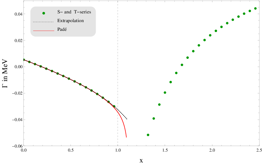
Refer to caption
Figure 15: Combined NNLO plot for the diagrams (f)\boldsymbol{(f)}, (g)\boldsymbol{(g)} and (h)\boldsymbol{(h)} including the SS-series, the TT-series, the extrapolation of the SS-series, the [5,4][5,4] Padé approximation of the SS-series and the interpolation of the SS- and TT-series. Every series is plotted up to 𝒪⁡(x±9)\mathcal{O}(x^{\pm 9}).
Refer to caption
Figure 16: Combined NNLO plot for the diagrams (f)\boldsymbol{(f)}, (g)\boldsymbol{(g)} and (h)\boldsymbol{(h)} on a larger scale including the SS-series, the extrapolation of the SS-series and the Padé approximation of the SS-series. The SS-series and the extrapolation are plotted up to 𝒪⁡(x±7)\mathcal{O}(x^{\pm 7}), 𝒪⁡(x±8)\mathcal{O}(x^{\pm 8}) and 𝒪⁡(x±9)\mathcal{O}(x^{\pm 9}) corresponding to the three curves from top to bottom, respectively. The [4,3][4,3], [4,4][4,4] and [5,4][5,4] Padé approximations correspond to the three curves from top to bottom. The error bar serves to determine the uncertainty of the result in Section 3.

A General Results: Coefficients for 𝑴𝑾≠𝑴𝒁\boldsymbol{M_{W}\neq M_{Z}}

As outlined in Sections 2.2 and 2.3, Eqs. (12) and (45) specify the results of the asymptotic expansions at NLO and NNLO only for the special case MW=MZM_{W}=M_{Z}. The general results can be obtained by adding expressions of the form (15) and (47) to every asymptotic series with a ZZ boson inside the loop, i.e. to the series of the groups (b)(b), (d)(d) and (e)(e) in Figs. 4 and 10. The coefficients an,ma_{n,m} and bn,mb_{n,m} belong to the NLO electroweak corrections of 𝒪⁡(α)\mathcal{O}(\alpha) and the NNLO mixed QCD/electroweak corrections of 𝒪⁡(α​αs)\mathcal{O}(\alpha\,\alpha_{s}) and will be presented in Sections A.1 and A.2, respectively. Within one group (b)(b), (d)(d) or (e)(e), these coefficients are accompanied by the same prefactor PP, which is split off according to

an,m=P⋅An,m,bn,m=P⋅Bn,m.a_{n,m}=P\cdot A_{n,m}\,,\quad b_{n,m}=P\cdot B_{n,m}\,. (A.1)

PP agrees with the prefactors of the corresponding ss-series in Eqs. (12) and (45) and will be indicated individually.

A.1 Next-To-Leading-Order Decay Width:
Electroweak Corrections of Order 𝜶\boldsymbol{\alpha}

Coefficients of group (b)(b): P=cw/sw​(gq−gq′)P=c_{w}/s_{w}\,\left(g_{q}-g_{q^{\prime}}\right)

A0,1\displaystyle A_{0,1} =34,A0,2=14,A0,3=18,A0,4=340,A0,5=120,A0,6=128,A0,7=3112,A0,8=148,\displaystyle=\frac{3}{4}\,,A_{0,2}=\frac{1}{4}\,,A_{0,3}=\frac{1}{8}\,,A_{0,4}=\frac{3}{40}\,,A_{0,5}=\frac{1}{20}\,,A_{0,6}=\frac{1}{28}\,,A_{0,7}=\frac{3}{112}\,,A_{0,8}=\frac{1}{48}\,,
A0,9\displaystyle A_{0,9} =160,A0,10=3220,\displaystyle=\frac{1}{60}\,,A_{0,10}=\frac{3}{220}\,,
A1,1\displaystyle A_{1,1} =−536,A1,2=−110,A1,3=−29360,A1,4=−43630,A1,5=−584,A1,6=−10189,\displaystyle=-\frac{5}{36}\,,A_{1,2}=-\frac{1}{10}\,,A_{1,3}=-\frac{29}{360}\,,A_{1,4}=-\frac{43}{630}\,,A_{1,5}=-\frac{5}{84}\,,A_{1,6}=-\frac{10}{189}\,,
A1,7\displaystyle A_{1,7} =−1032160,A1,8=−43990,A1,9=−791980,\displaystyle=-\frac{103}{2160}\,,A_{1,8}=-\frac{43}{990}\,,A_{1,9}=-\frac{79}{1980}\,,
A2,1\displaystyle A_{2,1} =−5144,A2,2=−9280,A2,3=−1495040,A2,4=−552016,A2,5=−17672,A2,6=−7297,\displaystyle=-\frac{5}{144}\,,A_{2,2}=-\frac{9}{280}\,,A_{2,3}=-\frac{149}{5040}\,,A_{2,4}=-\frac{55}{2016}\,,A_{2,5}=-\frac{17}{672}\,,A_{2,6}=-\frac{7}{297}\,,
A2,7\displaystyle A_{2,7} =−1315940,A2,8=−23711440,\displaystyle=-\frac{131}{5940}\,,A_{2,8}=-\frac{237}{11440}\,,
A3,1\displaystyle A_{3,1} =−232800,A3,2=−1105,A3,3=−171680,A3,4=−19118480,A3,5=−91880,\displaystyle=-\frac{23}{2800}\,,A_{3,2}=-\frac{1}{105}\,,A_{3,3}=-\frac{17}{1680}\,,A_{3,4}=-\frac{191}{18480}\,,A_{3,5}=-\frac{91}{880}\,,
A3,6\displaystyle A_{3,6} =−32932175,A3,7=−20120020,\displaystyle=-\frac{329}{32175}\,,A_{3,7}=-\frac{201}{20020}\,,
A4,1\displaystyle A_{4,1} =−7337800,A4,2=−51848,A4,3=−547166320,A4,4=−28777220,A4,5=−25964350,\displaystyle=-\frac{73}{37800}\,,A_{4,2}=-\frac{5}{1848}\,,A_{4,3}=-\frac{547}{166320}\,,A_{4,4}=-\frac{287}{77220}\,,A_{4,5}=-\frac{259}{64350}\,,
A4,6\displaystyle A_{4,6} =−71650,\displaystyle=-\frac{7}{1650}\,,
A5,1\displaystyle A_{5,1} =−53116424,A5,2=−34004,A5,3=−445432432,A5,4=−173135135,A5,5=−32002,\displaystyle=-\frac{53}{116424}\,,A_{5,2}=-\frac{3}{4004}\,,A_{5,3}=-\frac{445}{432432}\,,A_{5,4}=-\frac{173}{135135}\,,A_{5,5}=-\frac{3}{2002}\,,
A6,1\displaystyle A_{6,1} =−1451345344,A6,2=−734320,A6,3=−41131040,A6,4=−23195445440,\displaystyle=-\frac{145}{1345344}\,,A_{6,2}=-\frac{7}{34320}\,,A_{6,3}=-\frac{41}{131040}\,,A_{6,4}=-\frac{2319}{5445440}\,,
A7,1\displaystyle A_{7,1} =−19741312,A7,2=−236465,A7,3=−97710501920,\displaystyle=-\frac{19}{741312}\,,A_{7,2}=-\frac{2}{36465}\,,A_{7,3}=-\frac{977}{10501920}\,,
A8,1\displaystyle A_{8,1} =−24139382200,A8,2=−271847560,\displaystyle=-\frac{241}{39382200}\,,A_{8,2}=-\frac{27}{1847560}\,,
A9,1\displaystyle A_{9,1} =−149101615800.\displaystyle=-\frac{149}{101615800}\,. (A.2)

Coefficients of group (d)(d): P=gq2+gq′2P=g_{q}^{2}+g_{q^{\prime}}^{2}

A0,1\displaystyle A_{0,1} =−14,A0,2=−18,A0,3=−112,A0,4=−116,A0,5=−120,A0,6=−124,A0,7=−128,\displaystyle=-\frac{1}{4}\,,A_{0,2}=-\frac{1}{8}\,,A_{0,3}=-\frac{1}{12}\,,A_{0,4}=-\frac{1}{16}\,,A_{0,5}=-\frac{1}{20}\,,A_{0,6}=-\frac{1}{24}\,,A_{0,7}=-\frac{1}{28}\,,
A0,8\displaystyle A_{0,8} =−132,A0,9=−136,A0,10=−140,\displaystyle=-\frac{1}{32}\,,A_{0,9}=-\frac{1}{36}\,,A_{0,10}=-\frac{1}{40}\,,
A1,m\displaystyle A_{1,m} =0,\displaystyle=0\,,
A2,m\displaystyle A_{2,m} =0,\displaystyle=0\,,
A3,m\displaystyle A_{3,m} =0,\displaystyle=0\,,
A4,m\displaystyle A_{4,m} =0,\displaystyle=0\,,
A5,m\displaystyle A_{5,m} =0,\displaystyle=0\,,
A6,m\displaystyle A_{6,m} =0,\displaystyle=0\,,
A7,m\displaystyle A_{7,m} =0,\displaystyle=0\,,
A8,m\displaystyle A_{8,m} =0,\displaystyle=0\,,
A9,m\displaystyle A_{9,m} =0.\displaystyle=0\,. (A.3)

Coefficients of group (e)(e): P=gq​gq′P=g_{q}\,g_{q^{\prime}}

A0,1\displaystyle A_{0,1} =12,A0,2=14,A0,3=16,A0,4=18,A0,5=110,A0,6=112,A0,7=114,A0,8=116,\displaystyle=\frac{1}{2}\,,A_{0,2}=\frac{1}{4}\,,A_{0,3}=\frac{1}{6}\,,A_{0,4}=\frac{1}{8}\,,A_{0,5}=\frac{1}{10}\,,A_{0,6}=\frac{1}{12}\,,A_{0,7}=\frac{1}{14}\,,A_{0,8}=\frac{1}{16}\,,
A0,9\displaystyle A_{0,9} =118,A0,10=120,\displaystyle=\frac{1}{18}\,,A_{0,10}=\frac{1}{20}\,,
A1,1\displaystyle A_{1,1} =518−13​ln​x,A1,2=19−13​ln​x,A1,3=−13​ln​x,A1,4=−112−13​ln​x,\displaystyle=\frac{5}{18}-\frac{1}{3}\,\mathrm{ln}\,x\,,A_{1,2}=\frac{1}{9}-\frac{1}{3}\,\mathrm{ln}\,x\,,A_{1,3}=-\frac{1}{3}\,\mathrm{ln}\,x\,,A_{1,4}=-\frac{1}{12}-\frac{1}{3}\,\mathrm{ln}\,x\,,
A1,5\displaystyle A_{1,5} =−320−13​ln​x,A1,6=−37180−13​ln​x,A1,7=−3191260−13​ln​x,\displaystyle=-\frac{3}{20}-\frac{1}{3}\,\mathrm{ln}\,x\,,A_{1,6}=-\frac{37}{180}-\frac{1}{3}\,\mathrm{ln}\,x\,,A_{1,7}=-\frac{319}{1260}-\frac{1}{3}\,\mathrm{ln}\,x\,,
A1,8\displaystyle A_{1,8} =−7432520−13​ln​x,A1,9=−25097560−13​ln​x,\displaystyle=-\frac{743}{2520}-\frac{1}{3}\,\mathrm{ln}\,x\,,A_{1,9}=-\frac{2509}{7560}-\frac{1}{3}\,\mathrm{ln}\,x\,,
A2,1\displaystyle A_{2,1} =−772+16​ln​x,A2,2=−116+14​ln​x,A2,3=13​ln​x,A2,4=112+512​ln​x,\displaystyle=-\frac{7}{72}+\frac{1}{6}\,\mathrm{ln}\,x\,,A_{2,2}=-\frac{1}{16}+\frac{1}{4}\,\mathrm{ln}\,x\,,A_{2,3}=\frac{1}{3}\,\mathrm{ln}\,x\,,A_{2,4}=\frac{1}{12}+\frac{5}{12}\,\mathrm{ln}\,x\,,
A2,5\displaystyle A_{2,5} =1160+12​ln​x,A2,6=107360+712​ln​x,A2,7=5331260+23​ln​x,A2,8=18793360+34​ln​x,\displaystyle=\frac{11}{60}+\frac{1}{2}\,\mathrm{ln}\,x\,,A_{2,6}=\frac{107}{360}+\frac{7}{12}\,\mathrm{ln}\,x\,,A_{2,7}=\frac{533}{1260}+\frac{2}{3}\,\mathrm{ln}\,x\,,A_{2,8}=\frac{1879}{3360}+\frac{3}{4}\,\mathrm{ln}\,x\,,
A3,1\displaystyle A_{3,1} =9200−110​ln​x,A3,2=125−15​ln​x,A3,3=−13​ln​x,A3,4=−112−12​ln​x,\displaystyle=\frac{9}{200}-\frac{1}{10}\,\mathrm{ln}\,x\,,A_{3,2}=\frac{1}{25}-\frac{1}{5}\,\mathrm{ln}\,x\,,A_{3,3}=-\frac{1}{3}\,\mathrm{ln}\,x\,,A_{3,4}=-\frac{1}{12}-\frac{1}{2}\,\mathrm{ln}\,x\,,
A3,5\displaystyle A_{3,5} =−1360−710​ln​x,A3,6=−73180−1415​ln​x,A3,7=−5584−65​ln​x,\displaystyle=-\frac{13}{60}-\frac{7}{10}\,\mathrm{ln}\,x\,,A_{3,6}=-\frac{73}{180}-\frac{14}{15}\,\mathrm{ln}\,x\,,A_{3,7}=-\frac{55}{84}-\frac{6}{5}\,\mathrm{ln}\,x\,,
A4,1\displaystyle A_{4,1} =−11450+115​ln​x,A4,2=−136+16​ln​x,A4,3=13​ln​x,A4,4=112+712​ln​x,\displaystyle=-\frac{11}{450}+\frac{1}{15}\,\mathrm{ln}\,x\,,A_{4,2}=-\frac{1}{36}+\frac{1}{6}\,\mathrm{ln}\,x\,,A_{4,3}=\frac{1}{3}\,\mathrm{ln}\,x\,,A_{4,4}=\frac{1}{12}+\frac{7}{12}\,\mathrm{ln}\,x\,,
A4,5\displaystyle A_{4,5} =14+1415​ln​x,A4,6=191360+75​ln​x,\displaystyle=\frac{1}{4}+\frac{14}{15}\,\mathrm{ln}\,x\,,A_{4,6}=\frac{191}{360}+\frac{7}{5}\,\mathrm{ln}\,x\,,
A5,1\displaystyle A_{5,1} =13882−121​ln​x,A5,2=149−17​ln​x,A5,3=−13​ln​x,A5,4=−112−23​ln​x,\displaystyle=\frac{13}{882}-\frac{1}{21}\,\mathrm{ln}\,x\,,A_{5,2}=\frac{1}{49}-\frac{1}{7}\,\mathrm{ln}\,x\,,A_{5,3}=-\frac{1}{3}\,\mathrm{ln}\,x\,,A_{5,4}=-\frac{1}{12}-\frac{2}{3}\,\mathrm{ln}\,x\,,
A5,5\displaystyle A_{5,5} =−1760−65​ln​x,\displaystyle=-\frac{17}{60}-\frac{6}{5}\,\mathrm{ln}\,x\,,
A6,1\displaystyle A_{6,1} =−151568+128​ln​x,A6,2=−164+18​ln​x,A6,3=13​ln​x,A6,4=112+34​ln​x,\displaystyle=-\frac{15}{1568}+\frac{1}{28}\,\mathrm{ln}\,x\,,A_{6,2}=-\frac{1}{64}+\frac{1}{8}\,\mathrm{ln}\,x\,,A_{6,3}=\frac{1}{3}\,\mathrm{ln}\,x\,,A_{6,4}=\frac{1}{12}+\frac{3}{4}\,\mathrm{ln}\,x\,,
A7,1\displaystyle A_{7,1} =172592−136​ln​x,A7,2=181−19​ln​x,A7,3=−13​ln​x,\displaystyle=\frac{17}{2592}-\frac{1}{36}\,\mathrm{ln}\,x\,,A_{7,2}=\frac{1}{81}-\frac{1}{9}\,\mathrm{ln}\,x\,,A_{7,3}=-\frac{1}{3}\,\mathrm{ln}\,x\,, (A.4)
A8,1\displaystyle A_{8,1} =−194050+145​ln​x,A8,2=−1100+110​ln​x,\displaystyle=-\frac{19}{4050}+\frac{1}{45}\,\mathrm{ln}\,x\,,A_{8,2}=-\frac{1}{100}+\frac{1}{10}\,\mathrm{ln}\,x\,,
A9,1\displaystyle A_{9,1} =216050−155​ln​x.\displaystyle=\frac{21}{6050}-\frac{1}{55}\,\mathrm{ln}\,x\,. (A.4)

A.2 Next-To-Next-To-Leading-Order Decay Width:
Mixed QCD/Electroweak Corrections of Order 𝜶​𝜶𝒔\boldsymbol{\alpha\,\alpha_{s}}

Coefficients of group (b)(b): P=cw/sw​(gq−gq′)P=c_{w}/s_{w}\,\left(g_{q}-g_{q^{\prime}}\right)

B0,1\displaystyle B_{0,1} =12,B0,2=16,B0,3=112,B0,4=120,B0,5=130,\displaystyle=\frac{1}{2}\,,B_{0,2}=\frac{1}{6}\,,B_{0,3}=\frac{1}{12}\,,B_{0,4}=\frac{1}{20}\,,B_{0,5}=\frac{1}{30}\,,
B1,1\displaystyle B_{1,1} =−736,B1,2=−73540,B1,3=−19180,B1,4=−11126,B1,5=−1131512,\displaystyle=-\frac{7}{36}\,,B_{1,2}=-\frac{73}{540}\,,B_{1,3}=-\frac{19}{180}\,,B_{1,4}=-\frac{11}{126}\,,B_{1,5}=-\frac{113}{1512}\,,
B2,1\displaystyle B_{2,1} =−892160,B2,2=−1273360,B2,3=−13378,B2,4=−953024,B2,5=−973360,\displaystyle=-\frac{89}{2160}\,,B_{2,2}=-\frac{127}{3360}\,,B_{2,3}=-\frac{13}{378}\,,B_{2,4}=-\frac{95}{3024}\,,B_{2,5}=-\frac{97}{3360}\,,
B3,1\displaystyle B_{3,1} =−293150,B3,2=−676300,B3,3=−171512,B3,4=−958316,B3,5=−1351118800,\displaystyle=-\frac{29}{3150}\,,B_{3,2}=-\frac{67}{6300}\,,B_{3,3}=-\frac{17}{1512}\,,B_{3,4}=-\frac{95}{8316}\,,B_{3,5}=-\frac{1351}{118800}\,,
B4,1\displaystyle B_{4,1} =−5325200,B4,2=−587199584,B4,3=−593166320,B4,4=−49631235520,B4,5=−50231158300,\displaystyle=-\frac{53}{25200}\,,B_{4,2}=-\frac{587}{199584}\,,B_{4,3}=-\frac{593}{166320}\,,B_{4,4}=-\frac{4963}{1235520}\,,B_{4,5}=-\frac{5023}{1158300}\,,
B5,1\displaystyle B_{5,1} =−8511746360,B5,2=−20212522520,B5,3=−509463320,B5,4=−7957915,\displaystyle=-\frac{851}{1746360}\,,B_{5,2}=-\frac{2021}{2522520}\,,B_{5,3}=-\frac{509}{463320}\,,B_{5,4}=-\frac{79}{57915}\,,
B6,1\displaystyle B_{6,1} =−138112108096,B6,2=−41190080,B6,3=−134405405,\displaystyle=-\frac{1381}{12108096}\,,B_{6,2}=-\frac{41}{190080}\,,B_{6,3}=-\frac{134}{405405}\,,
B7,1\displaystyle B_{7,1} =−34912972960,B7,2=−475982702620,\displaystyle=-\frac{349}{12972960}\,,B_{7,2}=-\frac{4759}{82702620}\,,
B8,1\displaystyle B_{8,1} =−3017472586400.\displaystyle=-\frac{3017}{472586400}\,. (A.5)

Coefficients of group (d)(d): P=gq2+gq′2P=g_{q}^{2}+g_{q^{\prime}}^{2}

B0,m\displaystyle B_{0,m} =0\displaystyle=0
B1,1\displaystyle B_{1,1} =−55243+1681​ln​x−127​ln2​x,B1,2=−31243+1381​ln​x−127​ln2​x,\displaystyle=-\frac{55}{243}+\frac{16}{81}\,\mathrm{ln}\,x-\frac{1}{27}\,\mathrm{ln}^{2}\,x\,,B_{1,2}=-\frac{31}{243}+\frac{13}{81}\,\mathrm{ln}\,x-\frac{1}{27}\,\mathrm{ln}^{2}\,x\,,
B1,3\displaystyle B_{1,3} =−227+1181​ln​x−127​ln2​x,B1,4=−13324+19162​ln​x−127​ln2​x,\displaystyle=-\frac{2}{27}+\frac{11}{81}\,\mathrm{ln}\,x-\frac{1}{27}\,\mathrm{ln}^{2}\,x\,,B_{1,4}=-\frac{13}{324}+\frac{19}{162}\,\mathrm{ln}\,x-\frac{1}{27}\,\mathrm{ln}^{2}\,x\,,
B1,5\displaystyle B_{1,5} =−160+83810​ln​x−127​ln2​x,\displaystyle=-\frac{1}{60}+\frac{83}{810}\,\mathrm{ln}\,x-\frac{1}{27}\,\mathrm{ln}^{2}\,x\,,
B2,1\displaystyle B_{2,1} =−917776+5324​ln​x−1216​ln2​x,B2,2=−171728+154​ln​x−1144​ln2​x,\displaystyle=-\frac{91}{7776}+\frac{5}{324}\,\mathrm{ln}\,x-\frac{1}{216}\,\mathrm{ln}^{2}\,x\,,B_{2,2}=-\frac{17}{1728}+\frac{1}{54}\,\mathrm{ln}\,x-\frac{1}{144}\,\mathrm{ln}^{2}\,x\,,
B2,3\displaystyle B_{2,3} =−1144+13648​ln​x−1108​ln2​x,B2,4=−195184+532592​ln​x−5432​ln2​x,\displaystyle=-\frac{1}{144}+\frac{13}{648}\,\mathrm{ln}\,x-\frac{1}{108}\,\mathrm{ln}^{2}\,x\,,B_{2,4}=-\frac{19}{5184}+\frac{53}{2592}\,\mathrm{ln}\,x-\frac{5}{432}\,\mathrm{ln}^{2}\,x\,,
B2,5\displaystyle B_{2,5} =−13240+432160​ln​x−172​ln2​x,\displaystyle=-\frac{1}{3240}+\frac{43}{2160}\,\mathrm{ln}\,x-\frac{1}{72}\,\mathrm{ln}^{2}\,x\,,
B3,1\displaystyle B_{3,1} =−4730000+3713500​ln​x−1900​ln2​x,B3,2=−11967500+5913500​ln​x−1450​ln2​x,\displaystyle=-\frac{47}{30000}+\frac{37}{13500}\,\mathrm{ln}\,x-\frac{1}{900}\,\mathrm{ln}^{2}\,x\,,B_{3,2}=-\frac{119}{67500}+\frac{59}{13500}\,\mathrm{ln}\,x-\frac{1}{450}\,\mathrm{ln}^{2}\,x\,,
B3,3\displaystyle B_{3,3} =−1675+478100​ln​x−1270​ln2​x,B3,4=−11296+375400​ln​x−1180​ln2​x,\displaystyle=-\frac{1}{675}+\frac{47}{8100}\,\mathrm{ln}\,x-\frac{1}{270}\,\mathrm{ln}^{2}\,x\,,B_{3,4}=-\frac{1}{1296}+\frac{37}{5400}\,\mathrm{ln}\,x-\frac{1}{180}\,\mathrm{ln}^{2}\,x\,,
B3,5\displaystyle B_{3,5} =47162000+19927000​ln​x−7900​ln2​x,\displaystyle=\frac{47}{162000}+\frac{199}{27000}\,\mathrm{ln}\,x-\frac{7}{900}\,\mathrm{ln}^{2}\,x\,, (A.6)
B4,1\displaystyle B_{4,1} =−4071215000+5981000​ln​x−12700​ln2​x,B4,2=−2348600+4732400​ln​x−11080​ln2​x,\displaystyle=-\frac{407}{1215000}+\frac{59}{81000}\,\mathrm{ln}\,x-\frac{1}{2700}\,\mathrm{ln}^{2}\,x\,,B_{4,2}=-\frac{23}{48600}+\frac{47}{32400}\,\mathrm{ln}\,x-\frac{1}{1080}\,\mathrm{ln}^{2}\,x\,,
B4,3\displaystyle B_{4,3} =−12160+3716200​ln​x−1540​ln2​x,B4,4=−31129600+19964800​ln​x−72160​ln2​x,\displaystyle=-\frac{1}{2160}+\frac{37}{16200}\,\mathrm{ln}\,x-\frac{1}{540}\,\mathrm{ln}^{2}\,x\,,B_{4,4}=-\frac{31}{129600}+\frac{199}{64800}\,\mathrm{ln}\,x-\frac{7}{2160}\,\mathrm{ln}^{2}\,x\,,
B4,5\displaystyle B_{4,5} =14320+29381000​ln​x−71350​ln2​x,\displaystyle=\frac{1}{4320}+\frac{293}{81000}\,\mathrm{ln}\,x-\frac{7}{1350}\,\mathrm{ln}^{2}\,x\,,
B5,1\displaystyle B_{5,1} =−139114586075+172694575​ln​x−16615​ln2​x,\displaystyle=-\frac{1391}{14586075}+\frac{172}{694575}\,\mathrm{ln}\,x-\frac{1}{6615}\,\mathrm{ln}^{2}\,x\,,
B5,2\displaystyle B_{5,2} =−2631620675+137231525​ln​x−12205​ln2​x,B5,3=−211025+10799225​ln​x−1945​ln2​x,\displaystyle=-\frac{263}{1620675}+\frac{137}{231525}\,\mathrm{ln}\,x-\frac{1}{2205}\,\mathrm{ln}^{2}\,x\,,B_{5,3}=-\frac{2}{11025}+\frac{107}{99225}\,\mathrm{ln}\,x-\frac{1}{945}\,\mathrm{ln}^{2}\,x\,,
B5,4\displaystyle B_{5,4} =−37396900+323198450​ln​x−2945​ln2​x,\displaystyle=-\frac{37}{396900}+\frac{323}{198450}\,\mathrm{ln}\,x-\frac{2}{945}\,\mathrm{ln}^{2}\,x\,,
B6,1\displaystyle B_{6,1} =−36511063808+59592704​ln​x−114112​ln2​x,\displaystyle=-\frac{365}{11063808}+\frac{59}{592704}\,\mathrm{ln}\,x-\frac{1}{14112}\,\mathrm{ln}^{2}\,x\,,
B6,2\displaystyle B_{6,2} =−891354752+47169344​ln​x−14032​ln2​x,B6,3=−112096+73127008​ln​x−11512​ln2​x,\displaystyle=-\frac{89}{1354752}+\frac{47}{169344}\,\mathrm{ln}\,x-\frac{1}{4032}\,\mathrm{ln}^{2}\,x\,,B_{6,3}=-\frac{1}{12096}+\frac{73}{127008}\,\mathrm{ln}\,x-\frac{1}{1512}\,\mathrm{ln}^{2}\,x\,,
B7,1\displaystyle B_{7,1} =−3247246903552+1553429216​ln​x−127216​ln2​x,\displaystyle=-\frac{3247}{246903552}+\frac{155}{3429216}\,\mathrm{ln}\,x-\frac{1}{27216}\,\mathrm{ln}^{2}\,x\,,
B7,2\displaystyle B_{7,2} =−46315431472+2471714608​ln​x−16804​ln2​x,\displaystyle=-\frac{463}{15431472}+\frac{247}{1714608}\,\mathrm{ln}\,x-\frac{1}{6804}\,\mathrm{ln}^{2}\,x\,,
B8,1\displaystyle B_{8,1} =−2299393660000+1978748000​ln​x−148600​ln2​x.\displaystyle=-\frac{2299}{393660000}+\frac{197}{8748000}\,\mathrm{ln}\,x-\frac{1}{48600}\,\mathrm{ln}^{2}\,x\,. (A.6)

Coefficients of group (e)(e): P=gq​gq′P=g_{q}\,g_{q^{\prime}}

B0,m\displaystyle B_{0,m} =0,\displaystyle=0\,,
B1,1\displaystyle B_{1,1} =5327−43​ζ​(3)−43​ln​x−13​ln2​x,B1,2=3527−43​ζ​(3)−53​ln​x−13​ln2​x,\displaystyle=\frac{53}{27}-\frac{4}{3}\,\zeta(3)-\frac{4}{3}\,\mathrm{ln}\,x-\frac{1}{3}\,\mathrm{ln}^{2}\,x\,,B_{1,2}=\frac{35}{27}-\frac{4}{3}\,\zeta(3)-\frac{5}{3}\,\mathrm{ln}\,x-\frac{1}{3}\,\mathrm{ln}^{2}\,x\,,
B1,3\displaystyle B_{1,3} =2027−43​ζ​(3)−179​ln​x−13​ln2​x,B1,4=29108−43​ζ​(3)−3718​ln​x−13​ln2​x,\displaystyle=\frac{20}{27}-\frac{4}{3}\,\zeta(3)-\frac{17}{9}\,\mathrm{ln}\,x-\frac{1}{3}\,\mathrm{ln}^{2}\,x\,,B_{1,4}=\frac{29}{108}-\frac{4}{3}\,\zeta(3)-\frac{37}{18}\,\mathrm{ln}\,x-\frac{1}{3}\,\mathrm{ln}^{2}\,x\,,
B1,5\displaystyle B_{1,5} =−77540−43​ζ​(3)−19790​ln​x−13​ln2​x,\displaystyle=-\frac{77}{540}-\frac{4}{3}\,\zeta(3)-\frac{197}{90}\,\mathrm{ln}\,x-\frac{1}{3}\,\mathrm{ln}^{2}\,x\,,
B2,1\displaystyle B_{2,1} =−791296+23​ζ​(3)+2318​ln​x−718​ln2​x,B2,2=473864+ζ⁡(3)+5536​ln​x−712​ln2​x,\displaystyle=-\frac{79}{1296}+\frac{2}{3}\,\zeta(3)+\frac{23}{18}\,\mathrm{ln}\,x-\frac{7}{18}\,\mathrm{ln}^{2}\,x\,,B_{2,2}=\frac{473}{864}+\zeta(3)+\frac{55}{36}\,\mathrm{ln}\,x-\frac{7}{12}\,\mathrm{ln}^{2}\,x\,,
B2,3\displaystyle B_{2,3} =803648+43​ζ​(3)+8954​ln​x−79​ln2​x,B2,4=50832592+53​ζ​(3)+361216​ln​x−3536​ln2​x,\displaystyle=\frac{803}{648}+\frac{4}{3}\,\zeta(3)+\frac{89}{54}\,\mathrm{ln}\,x-\frac{7}{9}\,\mathrm{ln}^{2}\,x\,,B_{2,4}=\frac{5083}{2592}+\frac{5}{3}\,\zeta(3)+\frac{361}{216}\,\mathrm{ln}\,x-\frac{35}{36}\,\mathrm{ln}^{2}\,x\,,
B2,5\displaystyle B_{2,5} =4316+2​ζ​(3)+9760​ln​x−76​ln2​x,\displaystyle=\frac{43}{16}+2\,\zeta(3)+\frac{97}{60}\,\mathrm{ln}\,x-\frac{7}{6}\,\mathrm{ln}^{2}\,x\,,
B3,1\displaystyle B_{3,1} =−7911200−25​ζ​(3)−1330​ln​x,B3,2=−307200−45​ζ​(3)−1315​ln​x,\displaystyle=-\frac{791}{1200}-\frac{2}{5}\,\zeta(3)-\frac{13}{30}\,\mathrm{ln}\,x\,,B_{3,2}=-\frac{307}{200}-\frac{4}{5}\,\zeta(3)-\frac{13}{15}\,\mathrm{ln}\,x\,,
B3,3\displaystyle B_{3,3} =−20572−43​ζ​(3)−139​ln​x,B3,4=−667144−2​ζ​(3)−136​ln​x,\displaystyle=-\frac{205}{72}-\frac{4}{3}\,\zeta(3)-\frac{13}{9}\,\mathrm{ln}\,x\,,B_{3,4}=-\frac{667}{144}-2\,\zeta(3)-\frac{13}{6}\,\mathrm{ln}\,x\,,
B3,5\displaystyle B_{3,5} =−4981720−145​ζ​(3)−9130​ln​x,\displaystyle=-\frac{4981}{720}-\frac{14}{5}\,\zeta(3)-\frac{91}{30}\,\mathrm{ln}\,x\,,
B4,1\displaystyle B_{4,1} =171079243000+415​ζ​(3)+233810​ln​x−1145​ln2​x,\displaystyle=\frac{171079}{243000}+\frac{4}{15}\,\zeta(3)+\frac{233}{810}\,\mathrm{ln}\,x-\frac{11}{45}\,\mathrm{ln}^{2}\,x\,,
B4,2\displaystyle B_{4,2} =18505997200+23​ζ​(3)+7691620​ln​x−1118​ln2​x,\displaystyle=\frac{185059}{97200}+\frac{2}{3}\,\zeta(3)+\frac{769}{1620}\,\mathrm{ln}\,x-\frac{11}{18}\,\mathrm{ln}^{2}\,x\,,
B4,3\displaystyle B_{4,3} =19274948600+43​ζ​(3)+439810​ln​x−119​ln2​x,\displaystyle=\frac{192749}{48600}+\frac{4}{3}\,\zeta(3)+\frac{439}{810}\,\mathrm{ln}\,x-\frac{11}{9}\,\mathrm{ln}^{2}\,x\,, (A.7)
B4,4\displaystyle B_{4,4} =1375583194400+73​ζ​(3)+10933240​ln​x−7736​ln2​x,\displaystyle=\frac{1375583}{194400}+\frac{7}{3}\,\zeta(3)+\frac{1093}{3240}\,\mathrm{ln}\,x-\frac{77}{36}\,\mathrm{ln}^{2}\,x\,,
B4,5\displaystyle B_{4,5} =2767561243000+5615​ζ​(3)−12794050​ln​x−15445​ln2​x,\displaystyle=\frac{2767561}{243000}+\frac{56}{15}\,\zeta(3)-\frac{1279}{4050}\,\mathrm{ln}\,x-\frac{154}{45}\,\mathrm{ln}^{2}\,x\,,
B5,1\displaystyle B_{5,1} =−1609923814−421​ζ​(3)−37567​ln​x,B5,2=−81793969−47​ζ​(3)−37189​ln​x,\displaystyle=-\frac{16099}{23814}-\frac{4}{21}\,\zeta(3)-\frac{37}{567}\,\mathrm{ln}\,x\,,B_{5,2}=-\frac{8179}{3969}-\frac{4}{7}\,\zeta(3)-\frac{37}{189}\,\mathrm{ln}\,x\,,
B5,3\displaystyle B_{5,3} =−82901701−43​ζ​(3)−3781​ln​x,B5,4=−670976804−83​ζ​(3)−7481​ln​x,\displaystyle=-\frac{8290}{1701}-\frac{4}{3}\,\zeta(3)-\frac{37}{81}\,\mathrm{ln}\,x\,,B_{5,4}=-\frac{67097}{6804}-\frac{8}{3}\,\zeta(3)-\frac{74}{81}\,\mathrm{ln}\,x\,,
B6,1\displaystyle B_{6,1} =529489097889056000+17​ζ​(3)+68915120​ln​x−143840​ln2​x,\displaystyle=\frac{529489097}{889056000}+\frac{1}{7}\,\zeta(3)+\frac{689}{15120}\,\mathrm{ln}\,x-\frac{143}{840}\,\mathrm{ln}^{2}\,x\,,
B6,2\displaystyle B_{6,2} =535276697254016000+12​ζ​(3)−656048​ln​x−143240​ln2​x,\displaystyle=\frac{535276697}{254016000}+\frac{1}{2}\,\zeta(3)-\frac{65}{6048}\,\mathrm{ln}\,x-\frac{143}{240}\,\mathrm{ln}^{2}\,x\,,
B6,3\displaystyle B_{6,3} =53493544795256000+43​ζ​(3)−965922680​ln​x−14390​ln2​x,\displaystyle=\frac{534935447}{95256000}+\frac{4}{3}\,\zeta(3)-\frac{9659}{22680}\,\mathrm{ln}\,x-\frac{143}{90}\,\mathrm{ln}^{2}\,x\,,
B7,1\displaystyle B_{7,1} =−259882013489888000−19​ζ​(3)+76319440​ln​x−71080​ln2​x,\displaystyle=-\frac{259882013}{489888000}-\frac{1}{9}\,\zeta(3)+\frac{763}{19440}\,\mathrm{ln}\,x-\frac{7}{1080}\,\mathrm{ln}^{2}\,x\,,
B7,2\displaystyle B_{7,2} =−257478563122472000−49​ζ​(3)+14639720​ln​x−7270​ln2​x,\displaystyle=-\frac{257478563}{122472000}-\frac{4}{9}\,\zeta(3)+\frac{1463}{9720}\,\mathrm{ln}\,x-\frac{7}{270}\,\mathrm{ln}^{2}\,x\,,
B8,1\displaystyle B_{8,1} =1391082879130005640000+445​ζ​(3)−526991701000​ln​x−4033150​ln2​x.\displaystyle=\frac{13910828791}{30005640000}+\frac{4}{45}\,\zeta(3)-\frac{52699}{1701000}\,\mathrm{ln}\,x-\frac{403}{3150}\,\mathrm{ln}^{2}\,x\,. (A.7)

References