跳到论文正文
W Papers独立论文阅读器 arXiv:1307.7176 论文正文 计算阅读时间 · 0%
引用这篇论文根据当前论文元数据生成,正式投稿前建议核对。


License: CC Zero
arXiv:1307.7176v1 [math.FA] 26 Jul 2013

Phase retrieval from very few measurements

Journal: Linear Algebra and its Applications
Matthew Fickus Address: Department of Mathematics and Statistics, Air Force Institute of Technology, Wright-Patterson AFB, OH 45433, USA    Dustin G. Mixon Email: dustin.mixon@afit.edu Address: Department of Mathematics and Statistics, Air Force Institute of Technology, Wright-Patterson AFB, OH 45433, USA    Aaron A. Nelson Address: Department of Mathematics and Statistics, Air Force Institute of Technology, Wright-Patterson AFB, OH 45433, USA    Yang Wang Address: Department of Mathematics, Michigan State University, East Lansing, MI 48824, USA
Abstract

In many applications, signals are measured according to a linear process, but the phases of these measurements are often unreliable or not available. To reconstruct the signal, one must perform a process known as phase retrieval. This paper focuses on completely determining signals with as few intensity measurements as possible, and on efficient phase retrieval algorithms from such measurements. For the case of complex MM-dimensional signals, we construct a measurement ensemble of size 4​M−44M-4 which yields injective intensity measurements; this is conjectured to be the smallest such ensemble. For the case of real signals, we devise a theory of “almost” injective intensity measurements, and we characterize such ensembles. Later, we show that phase retrieval from M+1M+1 almost injective intensity measurements is 𝖭𝖯{\mathsf{NP}}-hard, indicating that computationally efficient phase retrieval must come at the price of measurement redundancy.

Keywords: 
phase retrieval , informationally complete , unit norm tight frames , computational complexity

1 Introduction

Given an ensemble Φ={φn}n=1N\Phi=\{\varphi_{n}\}_{n=1}^{N} of MM-dimensional vectors (real or complex), the phase retrieval problem is to recover a signal xx from intensity measurements 𝒜⁡(x):={|⟨x,φn⟩|2}n=1N\mathcal{A}(x):=\{|\langle x,\varphi_{n}\rangle|^{2}\}_{n=1}^{N}. Note that for any scalar ω\omega of unit modulus, 𝒜⁡(ω​x)=𝒜⁡(x)\mathcal{A}(\omega x)=\mathcal{A}(x), and so the best one can hope to do is recover xx up to a global phase factor {ω​x:|ω|=1}\{\omega x:|\omega|=1\}. Intensity measurements arise in a number of applications in which phase is either unreliable or not available [9, 19, 27, 31, 32, 38], and in most of these applications, it is desirable to perform phase retrieval from as few measurements as possible; indeed, increasing NN invariably makes the measurement process more expensive or time consuming.

Recently, there has been a lot of work on algorithmic phase retrieval. For example, phase retrieval can be formulated as a low-rank (actually, rank-1) matrix recovery problem [11, 12, 13, 17, 21, 36], and with this formulation, phase retrieval is possible from N=O⁡(M)N=O(M) intensity measurements [12]. Another approach is to exploit the polarization identity along with expander graphs to design a measurement ensemble and apply spectral methods to perform phase retrieval [1, 5]. One can also formulate phase retrieval in terms of MaxCut, and solvers for this formulation are equivalent to a popular solver (PhaseLift) for the matrix recovery formulation [35, 37]. While this recent work has focused on stable and efficient phase retrieval from asymptotically few measurements (namely, N=O⁡(M)N=O(M)), the present paper focuses on injectivity and algorithmic efficiency with the absolute minimum number of measurements.

In the next section, we construct an ensemble of N=4​M−4N=4M-4 measurement vectors in ℂM\mathbb{C}^{M} which yield injective intensity measurements. This is the second known injective ensemble of this size (the first is due to Bodmann and Hammen [8]), and it is conjectured to be the smallest-possible injective ensemble [4]. The same conjecture suggests that 4​M−44M-4 generic measurement vectors yield injectivity (that is, there exists a measure-zero set of ensembles of 4​M−44M-4 vectors such that every ensemble of 4​M−44M-4 vectors outside of this set yields injectivity). The following summarizes what is currently known about the so-called “4​M−44M-4 conjecture”:

  • 1.

    The conjecture holds for M=2,3M=2,3 [4].

  • 2.

    If N<4​M−2​α​(M−1)−3N<4M-2\alpha(M-1)-3, then 𝒜\mathcal{A} is not injective [28]; here, α⁡(M−1)≤log2⁡M\alpha(M-1)\leq\log_{2}M denotes the number of 11’s in the binary expansion of M−1M-1.

  • 3.

    For each M≥2M\geq 2, there exists an ensemble Φ\Phi of N=4​M−4N=4M-4 measurement vectors such that 𝒜\mathcal{A} is injective [8] (see also Section 2 of this paper).

  • 4.

    If N≥4​M−2N\geq 4M-2, then 𝒜\mathcal{A} is injective for generic Φ\Phi [3].

Bodmann and Hammen [8] leverage the Dirichlet kernel and the Cayley map to prove injectivity of their ensemble, but it is unclear whether phase retrieval is algorithmically feasible from their ensemble. By contrast, for the ensemble in this paper, we use basic ideas from harmonic analysis over cyclic groups to devise a corresponding phase retrieval algorithm, and we demonstrate injectivity by proving that the algorithm succeeds.

In Section 3, we devise a theory of ensembles for which the corresponding intensity measurements are “almost” injective, that is, 𝒜−1​(𝒜⁡(x))={ω​x:|ω|=1}\mathcal{A}^{-1}(\mathcal{A}(x))=\{\omega x:|\omega|=1\} for almost every xx. In this section, we focus on the real case, meaning phase retrieval is up to a global sign factor ω=±1\omega=\pm 1, and our approach is inspired by the characterization of injectivity in the real case by Balan, Casazza and Edidin [3]. After characterizing almost injectivity in the real case, we find a particularly satisfying sufficient condition for almost injectivity: that Φ\Phi forms a unit norm tight frame with MM and NN relatively prime. Characterizing almost injectivity in the complex case remains an open problem.

We conclude with Section 4, in which we consider algorithmic phase retrieval in the real case from N=M+1N=M+1 almost injective intensity measurements. Specifically, we show that phase retrieval in this case is 𝖭𝖯{\mathsf{NP}}-hard by reduction from the subset sum problem. The hardness of phase retrieval in this minimal case suggests a new problem for phase retrieval: What is the smallest CC for which there exists a family of ensembles of size N=C​M+o⁡(M)N=CM+o(M) such that phase retrieval can be performed in polynomial time?

2 4​M−44M-4 injective intensity measurements

In this section, we provide an ensemble of 4​M−44M-4 measurement vectors which yield injective intensity measurements for ℂM\mathbb{C}^{M}. The vectors in our ensemble are modulated discrete cosine functions, and they are explicitly constructed at the end of this section. We start here by motivating our construction, specifically by identifying the significance of circular autocorrelation.

Consider the PP-dimensional complex vector space ℓ(ℤP):={u:ℤ→ℂ:u[p+P]=u[p],∀p∈ℤ}\ell(\mathbb{Z}_{P}):=\{u\colon\mathbb{Z}\rightarrow\mathbb{C}:u[p+P]=u[p],~\forall p\in\mathbb{Z}\}. The discrete Fourier basis in ℓ⁡(ℤP)\ell(\mathbb{Z}_{P}) is the sequence of PP vectors {fq}q∈ℤP\{f_{q}\}_{q\in\mathbb{Z}_{P}} defined by fq​[p]:=e2​π​i​p​q/Pf_{q}[p]:=e^{2\pi ipq/P} (the notation “q∈ℤPq\in\mathbb{Z}_{P}” is taken to mean a set of coset representatives of ℤ\mathbb{Z} with respect to the subgroup P​ℤP\mathbb{Z}). The discrete Fourier transform (DFT) on ℤP\mathbb{Z}_{P} is the analysis operator F∗:ℓ⁡(ℤP)→ℓ⁡(ℤP)F^{*}\colon\ell(\mathbb{Z}_{P})\rightarrow\ell(\mathbb{Z}_{P}) of this basis, with corresponding inverse DFT (F∗)−1=1P​F(F^{*})^{-1}=\frac{1}{P}F, where

(F∗u)[q]=⟨u,fq⟩=∑p∈ℤPu[p]e−2πipq/P,(Fv)[p]=∑q∈ℤPv[q]fq[p]=∑q∈ℤPv[q]e2​π​i​p​q/P.(F^{*}u)[q]=\langle u,f_{q}\rangle=\sum_{p\in\mathbb{Z}_{P}}u[p]e^{-2\pi ipq/P},\qquad(Fv)[p]=\sum_{q\in\mathbb{Z}_{P}}v[q]f_{q}[p]=\sum_{q\in\mathbb{Z}_{P}}v[q]e^{2\pi ipq/P}.

Now let Tp:ℓ⁡(ℤP)→ℓ⁡(ℤP)T^{p}\colon\ell(\mathbb{Z}_{P})\rightarrow\ell(\mathbb{Z}_{P}) be the translation operator defined by (Tp​u)​[p′]:=u⁡[p′−p](T^{p}u)[p^{\prime}]:=u[p^{\prime}-p]. The circular autocorrelation of uu is then CirAut⁡(u)∈ℓ⁡(ℤP)\operatorname{CirAut}(u)\in\ell(\mathbb{Z}_{P}), defined entrywise by

CirAut⁡(u)​[p]:=⟨u,Tp​u⟩=∑p′∈ℤPu⁡[p′]​u⁡[p′−p]¯.\operatorname{CirAut}(u)[p]:=\langle u,T^{p}u\rangle=\sum_{p^{\prime}\in\mathbb{Z}_{P}}u[p^{\prime}]\overline{u[p^{\prime}-p]}. (1)

Consider the DFT of a circular autocorrelation:

(F∗​CirAut⁡(u))​[q]\displaystyle(F^{*}\operatorname{CirAut}(u))[q] =∑p∈ℤP∑p′∈ℤPu[p′]u⁡[p′−p]¯e−2πipq/P\displaystyle=\sum_{p\in\mathbb{Z}_{P}}\sum_{p^{\prime}\in\mathbb{Z}_{P}}u[p^{\prime}]\overline{u[p^{\prime}-p]}e^{-2\pi ipq/P}
=∑p′∈ℤPu[p′]e−2πip′q/P(∑p∈ℤPu[p′−p]e−2πi(p′−p)q/P)¯\displaystyle=\sum_{p^{\prime}\in\mathbb{Z}_{P}}u[p^{\prime}]e^{-2\pi ip^{\prime}q/P}\overline{\bigg(\sum_{p\in\mathbb{Z}_{P}}u[p^{\prime}-p]e^{-2\pi i(p^{\prime}-p)q/P}\bigg)}
=∑p′∈ℤPu[p′]e−2πip′q/P(∑p′′∈ℤPu[p′′]e−2πip′′q/P)¯=|⟨u,fq⟩|2.\displaystyle=\sum_{p^{\prime}\in\mathbb{Z}_{P}}u[p^{\prime}]e^{-2\pi ip^{\prime}q/P}\overline{\bigg(\sum_{p^{\prime\prime}\in\mathbb{Z}_{P}}u[p^{\prime\prime}]e^{-2\pi ip^{\prime\prime}q/P}\bigg)}=|\langle u,f_{q}\rangle|^{2}.

As such, if one has the intensity measurements {|⟨u,fq⟩|2}q∈ℤP\{|\langle u,f_{q}\rangle|^{2}\}_{q\in\mathbb{Z}_{P}}, then one may compute the circular autocorrelation CirAut⁡(u)\operatorname{CirAut}(u) by applying the inverse DFT. In order to perform phase retrieval from {|⟨u,fq⟩|2}q∈ℤP\{|\langle u,f_{q}\rangle|^{2}\}_{q\in\mathbb{Z}_{P}}, it therefore suffices to determine uu from CirAut⁡(u)\operatorname{CirAut}(u). This is the motivation for our approach in this section.

To see how to “invert” CirAut\operatorname{CirAut}, let’s consider an example. Take x=(a,b,c)∈ℂ3x=(a,b,c)\in\mathbb{C}^{3} and consider the circular autocorrelation of xx as a signal in ℓ⁡(ℤ3)\ell(\mathbb{Z}_{3}):

CirAut⁡(x)=(|a|2+|b|2+|c|2,a​c¯+b​a¯+c​b¯,a​b¯+b​c¯+c​a¯).\displaystyle\operatorname{CirAut}(x)=(|a|^{2}+|b|^{2}+|c|^{2},a\overline{c}+b\overline{a}+c\overline{b},a\overline{b}+b\overline{c}+c\overline{a}).

Notice that every entry of CirAut⁡(x)\operatorname{CirAut}(x) is a nonlinear combination of the entries of xx, from which it is unclear how to compute the entries of xx. To simplify the structure, we pad xx with zeros and enforce even symmetry; then the circular autocorrelation of u:=(2​a,b,c,0,0,0,0,c,b)∈ℓ⁡(ℤ9)u:=(2a,b,c,0,0,0,0,c,b)\in\ell(\mathbb{Z}_{9}) is

CirAut⁡(u)=(4​|a|2CLOSE\displaystyle\operatorname{CirAut}(u)=(4|a|^{2} +|b|2+|c|2,2​Re⁡(2​a​b¯+b​c¯),|b|2+4​Re⁡(a​c¯),2​Re⁡(b​c¯),|c|2,\displaystyle+|b|^{2}+|c|^{2},2\operatorname{Re}(2a\overline{b}+b\overline{c}),|b|^{2}+4\operatorname{Re}(a\overline{c}),2\operatorname{Re}(b\overline{c}),|c|^{2},
OPEN|c|2,2​Re⁡(b​c¯),|b|2+4​Re⁡(a​c¯),2​Re⁡(2​a​b¯+b​c¯)).\displaystyle|c|^{2},2\operatorname{Re}(b\overline{c}),|b|^{2}+4\operatorname{Re}(a\overline{c}),2\operatorname{Re}(2a\overline{b}+b\overline{c})). (2)

Although it still appears rather complicated, this circular autocorrelation actually lends itself well to recovering the entries of xx.

Before explaining this further, first note that 9=4​(3)−39=4(3)-3, and we can generalize our mapping x↦ux\mapsto u by sending vectors in ℂM\mathbb{C}^{M} to members of ℓ⁡(ℤ4​M−3)\ell(\mathbb{Z}_{4M-3}). To make this clear, consider the reversal operator R:ℓ⁡(ℤP)→ℓ⁡(ℤP)R\colon\ell(\mathbb{Z}_{P})\rightarrow\ell(\mathbb{Z}_{P}) defined by (R​u)​[p]=u​[−p](Ru)[p]=u[-p]. Then given a vector x∈ℂMx\in\mathbb{C}^{M}, padding with zeros and enforcing even symmetry is equivalent to embedding xx in ℓ⁡(ℤ4​M−3)\ell(\mathbb{Z}_{4M-3}) by appending 3​M−33M-3 zeros to xx and then taking u=x+R​x∈ℓ⁡(ℤ4​M−3)u=x+Rx\in\ell(\mathbb{Z}_{4M-3}). (From this point forward we use xx to represent both the original signal in ℂM\mathbb{C}^{M} and the version of xx embedded in ℓ⁡(ℤ4​M−3)\ell(\mathbb{Z}_{4M-3}) via zero-padding; the distinction will be clear from context.) Computing x∈ℂMx\in\mathbb{C}^{M} then reduces to determining the first MM entries of x∈ℓ⁡(ℤ4​M−3)x\in\ell(\mathbb{Z}_{4M-3}) from CirAut⁡(x+R​x)\operatorname{CirAut}(x+Rx). If xx is completely real-valued, then this is indeed possible. For instance, consider the circular autocorrelation (2). If the entries of xx are all real, then this becomes

CirAut⁡(x+R​x)=(4​a2+b2+c2,4​a​b+2​b​c,b2+4​a​c,2​b​c,c2,c2,2​b​c,b2+4​a​c,4​a​b+2​b​c).\displaystyle\operatorname{CirAut}(x+Rx)=(4a^{2}+b^{2}+c^{2},4ab+2bc,b^{2}+4ac,2bc,c^{2},c^{2},2bc,b^{2}+4ac,4ab+2bc).

Since CirAut⁡(x+R​x)​[4]=c2\operatorname{CirAut}(x+Rx)[4]=c^{2}, we simply take a square root to obtain cc up to a sign. Assuming cc is nonzero, we then divide CirAut⁡(x+R​x)​[3]\operatorname{CirAut}(x+Rx)[3] by 2c to determine bb up to the same sign. Then subtracting b2b^{2} from CirAut⁡(x+R​x)​[2]\operatorname{CirAut}(x+Rx)[2] and dividing by 4​c4c gives aa up to the same sign.

From this example, we see that the process of recovering the entries of xx from CirAut⁡(x+R​x)\operatorname{CirAut}(x+Rx) is iterative, working backward through its first 2​M−22M-2 entries. But what happens if cc is zero? Fortunately, our process doesn’t break: In this case, we have

CirAut⁡(x+R​x)=(4​a2+b2,4​a​b,b2,0,0,0,0,b2,4​a​b).\displaystyle\operatorname{CirAut}(x+Rx)=(4a^{2}+b^{2},4ab,b^{2},0,0,0,0,b^{2},4ab).

Thus, we need only start with CirAut⁡(x+R​x)​[2]\operatorname{CirAut}(x+Rx)[2] to determine the remaining entries of xx up to a sign. This observation brings to light the important role of the last nonzero entry of xx in our iteration. The relationship between this coordinate and the entries of CirAut⁡(x+R​x)\operatorname{CirAut}(x+Rx) will become more rigorous later.

The above example illustrated how a real signal xx is determined by CirAut⁡(x+R​x)\operatorname{CirAut}(x+Rx). A complex-valued signal, on the other hand, is not completely determined from CirAut⁡(x+R​x)\operatorname{CirAut}(x+Rx). Luckily, this can be fixed by introducing a second vector in ℓ⁡(ℤ4​M−3)\ell(\mathbb{Z}_{4M-3}) obtained from xx, and we will demonstrate this later, but for now we focus on x+R​xx+Rx. To this end, let’s first take a closer look at the entries of CirAut⁡(x+R​x)\operatorname{CirAut}(x+Rx). Since this circular autocorrelation has even symmetry by construction, we need only consider all entries of CirAut⁡(x+R​x)\operatorname{CirAut}(x+Rx) up to index 2​M−22M-2. This leads to the following lemma:

Lemma 1.

Let xx denote an MM-dimensional complex signal embedded in ℓ⁡(ℤ4​M−3)\ell(\mathbb{Z}_{4M-3}) such that x⁡[p]=0x[p]=0 for all p=M,…,4​M−4p=M,\ldots,4M-4. Then CirAut⁡(x+R​x)​[p]=2​Re⁡⟨x,Tp​x⟩+⟨x,R​T−p​x⟩\operatorname{CirAut}(x+Rx)[p]=2\operatorname{Re}\langle x,T^{p}x\rangle+\langle x,RT^{-p}x\rangle for all p=1,…,2​M−2p=1,\ldots,2M-2.

Proof.

First note that by the definition of the circular autocorrelation in (1) we have

CirAut⁡(x+R​x)​[p]=⟨x+R​x,Tp​(x+R​x)⟩=2​Re⁡⟨x,Tp​x⟩+⟨x,R​T−p​x⟩+⟨x,R​Tp​x⟩.\operatorname{CirAut}(x+Rx)[p]=\langle x+Rx,T^{p}(x+Rx)\rangle=2\operatorname{Re}\langle x,T^{p}x\rangle+\langle x,RT^{-p}x\rangle+\langle x,RT^{p}x\rangle.

Thus, to complete the proof it suffices to show that ⟨x,R​Tp​x⟩=0\langle x,RT^{p}x\rangle=0 for all p=1,…,2​M−2p=1,\ldots,2M-2. Since xx is only nonzero in its first MM entries, we have

⟨x,R​Tp​x⟩=∑p′=0M−1x⁡[p′]​(R​Tp​x)​[p′]¯=∑p′=0M−1x⁡[p′]​(Tp​x)​[−p′]¯=∑p′=0M−1x⁡[p′]​x⁡[−p′−p]¯,\langle x,RT^{p}x\rangle=\sum_{p^{\prime}=0}^{M-1}x[p^{\prime}]\overline{(RT^{p}x)[p^{\prime}]}=\sum_{p^{\prime}=0}^{M-1}x[p^{\prime}]\overline{(T^{p}x)[-p^{\prime}]}=\sum_{p^{\prime}=0}^{M-1}x[p^{\prime}]\overline{x[-p^{\prime}-p]},

where the summand is zero whenever −p′−p∉[0,M−1]-p^{\prime}-p\notin[0,M-1] modulo 4​M−34M-3. This is equivalent to having −p-p not lie in the Minkowski sum p′+[0,M−1]p^{\prime}+[0,M-1], and since p′∈[0,M−1]p^{\prime}\in[0,M-1] we see that ⟨x,R​Tp​x⟩=0\langle x,RT^{p}x\rangle=0 for all p=1,…,2​M−2p=1,\ldots,2M-2. ∎

As a consequence of Lemma 1, the following theorem expresses the entries of CirAut⁡(x+R​x)\operatorname{CirAut}(x+Rx) in terms of the entries of xx:

Theorem 2.

Let xx denote an MM-dimensional complex signal embedded in ℓ⁡(ℤ4​M−3)\ell(\mathbb{Z}_{4M-3}) such that x⁡[p]=0x[p]=0 for all p=M,…,4​M−4p=M,\ldots,4M-4. Then we have

CirAut⁡(x+R​x)​[p]={2​Re⁡(∑p′=p+12M−1x⁡[p′]​(x⁡[p′−p]¯+x⁡[p−p′]¯))if p is odd2​Re⁡(∑p′=p2+1M−1x⁡[p′]​(x⁡[p′−p]¯+x⁡[p−p′]¯))+|x⁡[p2]|2if p is even\displaystyle\operatorname{CirAut}(x+Rx)[p]=\begin{cases}\displaystyle{2\operatorname{Re}\bigg(\sum_{p^{\prime}=\frac{p+1}{2}}^{M-1}x[p^{\prime}](\overline{x[p^{\prime}-p]}+\overline{x[p-p^{\prime}]})\bigg)}&\;\text{if $p$ is odd}\\ \displaystyle{2\operatorname{Re}\bigg(\sum_{p^{\prime}=\frac{p}{2}+1}^{M-1}x[p^{\prime}](\overline{x[p^{\prime}-p]}+\overline{x[p-p^{\prime}]})\bigg)+\left|x[\tfrac{p}{2}]\right|^{2}}&\;\text{if $p$ is even}\end{cases} (3)

for all p=1,…,2​M−2p=1,\ldots,2M-2.

Proof.

We first use Lemma 1 to get

CirAut⁡(x+R​x)​[p]\displaystyle\operatorname{CirAut}(x+Rx)[p] =2​Re⁡⟨x,Tp​x⟩+⟨x,R​T−p​x⟩\displaystyle=2\operatorname{Re}\langle x,T^{p}x\rangle+\langle x,RT^{-p}x\rangle
=2​Re⁡(∑p′=0M−1x⁡[p′]​x⁡[p′−p]¯)+∑p′=0M−1x⁡[p′]​x⁡[p−p′]¯\displaystyle=2\operatorname{Re}\bigg(\sum_{p^{\prime}=0}^{M-1}x[p^{\prime}]\overline{x[p^{\prime}-p]}\bigg)+\sum_{p^{\prime}=0}^{M-1}x[p^{\prime}]\overline{x[p-p^{\prime}]}
=2​Re⁡(∑p′=pM−1x⁡[p′]​x⁡[p′−p]¯)+∑p′=max⁡{p−(M−1),0}min⁡{p,M−1}x⁡[p′]​x⁡[p−p′]¯,\displaystyle=2\operatorname{Re}\bigg(\sum_{p^{\prime}=p}^{M-1}x[p^{\prime}]\overline{x[p^{\prime}-p]}\bigg)+\sum_{p^{\prime}=\max\{p-(M-1),0\}}^{\min\{p,M-1\}}x[p^{\prime}]\overline{x[p-p^{\prime}]}, (4)

where the last equality takes into account that the first summand is nonzero only when p′−p∈[0,M−1]p^{\prime}-p\in[0,M-1] and the second summand is nonzero only when p−p′∈[0,M−1]p-p^{\prime}\in[0,M-1], i.e., when p′∈[p,p+(M−1)]p^{\prime}\in[p,p+(M-1)] and p′∈[p−(M−1),p]p^{\prime}\in[p-(M-1),p], respectively. To continue, we divide our analysis into cases.

For p=1,…,M−1p=1,\ldots,M-1, (4) gives

CirAut⁡(x+R​x)​[p]=2​Re⁡(∑p′=pM−1x⁡[p′]​x⁡[p′−p]¯)+∑p′=0px⁡[p′]​x⁡[p−p′]¯.\operatorname{CirAut}(x+Rx)[p]=2\operatorname{Re}\bigg(\sum_{p^{\prime}=p}^{M-1}x[p^{\prime}]\overline{x[p^{\prime}-p]}\bigg)+\sum_{p^{\prime}=0}^{p}x[p^{\prime}]\overline{x[p-p^{\prime}]}. (5)

If pp is odd we can then write

∑p′=0px⁡[p′]​x⁡[p−p′]¯\displaystyle\sum_{p^{\prime}=0}^{p}x[p^{\prime}]\overline{x[p-p^{\prime}]} =∑p′=0p−12x⁡[p′]​x⁡[p−p′]¯+∑p′=p+12px⁡[p′]​x⁡[p−p′]¯\displaystyle=\sum_{p^{\prime}=0}^{\frac{p-1}{2}}x[p^{\prime}]\overline{x[p-p^{\prime}]}+\sum_{p^{\prime}=\frac{p+1}{2}}^{p}x[p^{\prime}]\overline{x[p-p^{\prime}]}
=∑p′′=p+12px⁡[p−p′′]​x⁡[p′′]¯+∑p′=p+12px⁡[p′]​x⁡[p−p′]¯=2​Re⁡(∑p′=p+12px⁡[p′]​x⁡[p−p′]¯),\displaystyle=\sum_{p^{\prime\prime}=\frac{p+1}{2}}^{p}x[p-p^{\prime\prime}]\overline{x[p^{\prime\prime}]}+\sum_{p^{\prime}=\frac{p+1}{2}}^{p}x[p^{\prime}]\overline{x[p-p^{\prime}]}=2\operatorname{Re}\bigg(\sum_{p^{\prime}=\frac{p+1}{2}}^{p}x[p^{\prime}]\overline{x[p-p^{\prime}]}\bigg), (6)

while if pp is even we similarly write

∑p′=0px⁡[p′]​x⁡[p−p′]¯=2​Re⁡(∑p′=p2+1px⁡[p′]​x⁡[p−p′]¯)+|x⁡[p2]|2.\sum_{p^{\prime}=0}^{p}x[p^{\prime}]\overline{x[p-p^{\prime}]}=2\operatorname{Re}\bigg(\sum_{p^{\prime}=\frac{p}{2}+1}^{p}x[p^{\prime}]\overline{x[p-p^{\prime}]}\bigg)+\left|x\big[\tfrac{p}{2}\big]\right|^{2}. (7)

Substituting (6) and (7) into (5) then gives (3).

For the remaining case, p=M,…,2​M−2p=M,\ldots,2M-2 and (4) gives

CirAut⁡(x+R​x)​[p]=∑p′=p−(M−1)M−1x⁡[p′]​x⁡[p−p′]¯.\operatorname{CirAut}(x+Rx)[p]=\sum_{p^{\prime}=p-(M-1)}^{M-1}x[p^{\prime}]\overline{x[p-p^{\prime}]}. (8)

Similar to the previous case, taking pp to be odd yields

∑p′=p−(M−1)M−1x⁡[p′]​x⁡[p−p′]¯=2​Re⁡(∑p′=p+12M−1x⁡[p′]​x⁡[p−p′]¯),\sum_{p^{\prime}=p-(M-1)}^{M-1}x[p^{\prime}]\overline{x[p-p^{\prime}]}=2\operatorname{Re}\bigg(\sum_{p^{\prime}=\frac{p+1}{2}}^{M-1}x[p^{\prime}]\overline{x[p-p^{\prime}]}\bigg), (9)

while taking pp to be even yields

∑p′=p−(M−1)M−1x⁡[p′]​x⁡[p−p′]¯=2​Re⁡(∑p′=p2+1M−1x⁡[p′]​x⁡[p−p′]¯)+|x⁡[p2]|2,\sum_{p^{\prime}=p-(M-1)}^{M-1}x[p^{\prime}]\overline{x[p-p^{\prime}]}=2\operatorname{Re}\bigg(\sum_{p^{\prime}=\frac{p}{2}+1}^{M-1}x[p^{\prime}]\overline{x[p-p^{\prime}]}\bigg)+\left|x\big[\tfrac{p}{2}\big]\right|^{2}, (10)

and substituting (9) and (10) into (8) also gives (3). ∎

Notice (3) shows that each member of {CirAut⁡(x+R​x)​[p]}p=12​M−2\{\operatorname{CirAut}(x+Rx)[p]\}_{p=1}^{2M-2} can be written as a combination of the first MM entries of xx, but only those at or beyond the ⌈p2⌉\lceil\frac{p}{2}\rceilth index. As such, the index of the last nonzero entry of xx is closely related to that of the last nonzero entry of {CirAut⁡(x+R​x)​[p]}p=12​M−2\{\operatorname{CirAut}(x+Rx)[p]\}_{p=1}^{2M-2}. This corresponds to our observation earlier in the case of x∈ℝ3x\in\mathbb{R}^{3} where the third coordinate was assumed to be zero. We identify the relationship between the locations of these nonzero entries in the following lemma:

Lemma 3.

Let xx denote an MM-dimensional complex signal embedded in ℓ⁡(ℤ4​M−3)\ell(\mathbb{Z}_{4M-3}) such that x⁡[p]=0x[p]=0 for all p=M,…,4​M−4p=M,\ldots,4M-4. Then the last nonzero entry of {CirAut⁡(x+R​x)​[p]}p=02​M−2\{\operatorname{CirAut}(x+Rx)[p]\}_{p=0}^{2M-2} has index p=2​qp=2q, where qq is the index of the last nonzero entry of xx.

Proof.

If q≥1q\geq 1, then (3) gives that CirAut⁡(x+R​x)​[2​q]=|x⁡[q]|2≠0\operatorname{CirAut}(x+Rx)[2q]=|x[q]|^{2}\neq 0. Note that since x⁡[p′]=0x[p^{\prime}]=0 for every p′>qp^{\prime}>q, (3) also gives that CirAut⁡(x+R​x)​[p]=0\operatorname{CirAut}(x+Rx)[p]=0 for every p>2​qp>2q. For the remaining case where q=0q=0, (3) immediately gives that CirAut⁡(x+R​x)​[p]=0\operatorname{CirAut}(x+Rx)[p]=0 for every p≥1p\geq 1. To show that CirAut⁡(x+R​x)​[0]≠0\operatorname{CirAut}(x+Rx)[0]\neq 0 in this case, we apply the definition of circular autocorrelation (1):

CirAut⁡(x+R​x)​[0]=⟨x+R​x,x+R​x⟩=‖x+R​x‖2=|2​x​[0]|2≠0,\operatorname{CirAut}(x+Rx)[0]=\langle x+Rx,x+Rx\rangle=\|x+Rx\|^{2}=|2x[0]|^{2}\neq 0,

where the last equality uses the fact that xx is only supported at 00 since q=0q=0. ∎

As previously mentioned, we are unable to recover the entries of a complex signal xx solely from CirAut⁡(x+R​x)\operatorname{CirAut}(x+Rx). One way to address this is to rotate the entries of xx in the complex plane and also take the circular autocorrelation of this modified signal. If we rotate by an angle which is not an integer multiple of π\pi, this will produce new entries which are linearly independent from the corresponding entries of xx when viewed as vectors in the complex plane. As we will see, the problem of recovering the entries of xx then reduces to solving a linear system.

Take any (4​M−3)×(4​M−3)(4M-3)\times(4M-3) diagonal modulation operator EE whose diagonal entries {ωk}k=04​M−4\{\omega_{k}\}_{k=0}^{4M-4} are of unit modulus satisfying ωj​ωk¯∉ℝ\omega_{j}\overline{\omega_{k}}\notin\mathbb{R} for all j≠kj\neq k and consider the new vector E​x∈ℓ⁡(ℤ4​M−3)Ex\in\ell(\mathbb{Z}_{4M-3}). Then Theorem 2 gives

CirAut⁡(E​x+R​E​x)​[p]\displaystyle\operatorname{CirAut}(Ex+REx)[p]
={2​Re⁡(∑p′=p+12M−1ωp′​x​[p′]​(ωp′−p¯​x⁡[p′−p]¯+ωp−p′¯​x⁡[p−p′]¯))if p is odd2​Re⁡(∑p′=p2+1M−1ωp′​x​[p′]​(ωp′−p¯​x⁡[p′−p]¯+ωp−p′¯​x⁡[p−p′]¯))+|x⁡[p2]|2if p is even\displaystyle\qquad\qquad=\begin{cases}\displaystyle{2\operatorname{Re}\bigg(\sum_{p^{\prime}=\frac{p+1}{2}}^{M-1}\omega_{p^{\prime}}x[p^{\prime}](\overline{\omega_{p^{\prime}-p}}\overline{x[p^{\prime}-p]}+\overline{\omega_{p-p^{\prime}}}\overline{x[p-p^{\prime}]})\bigg)}&\;\text{if $p$ is odd}\\ \displaystyle{2\operatorname{Re}\bigg(\sum_{p^{\prime}=\frac{p}{2}+1}^{M-1}\omega_{p^{\prime}}x[p^{\prime}](\overline{\omega_{p^{\prime}-p}}\overline{x[p^{\prime}-p]}+\overline{\omega_{p-p^{\prime}}}\overline{x[p-p^{\prime}]})\bigg)+\left|x[\tfrac{p}{2}]\right|^{2}}&\;\text{if $p$ is even}\end{cases} (11)

for all p=1,…,2​M−2p=1,\ldots,2M-2. We will see that (3) and (11) together allow us to solve for the entries of xx (up to a global phase factor) by working iteratively backward through the entries of CirAut⁡(x+R​x)\operatorname{CirAut}(x+Rx) and CirAut⁡(E​x+R​E​x)\operatorname{CirAut}(Ex+REx). As alluded to earlier, each entry index forms a linear system which can be solved using the following lemma:

Lemma 4.

Let a,b∈ℂ∖{0}a,b\in\mathbb{C}\setminus\{0\} and ω∈ℂ∖ℝ\omega\in\mathbb{C}\setminus\mathbb{R} with |ω|=1|\omega|=1. Then

b=ia¯​Im⁡(ω)​(Re⁡(ω​a​b¯)−ω​Re⁡(a​b¯)).b=\frac{i}{\overline{a}\operatorname{Im}(\omega)}\big(\operatorname{Re}(\omega a\overline{b})-\omega\operatorname{Re}(a\overline{b})\big). (12)
Proof.

Define θ:=arg⁡(ω)\theta:=\operatorname{arg}(\omega) and ϕ:=arg⁡(a​b¯)\phi:=\operatorname{arg}(a\overline{b}). Then θ+ϕ≡arg⁡(ω​a​b)mod2​π\theta+\phi\equiv\operatorname{arg}(\omega ab)\bmod 2\pi and

cos⁡(ϕ)=Re⁡(a​b¯)|a​b¯|,sin⁡(ϕ)=Im⁡(a​b¯)|a​b¯|,cos⁡(θ+ϕ)=Re⁡(ω​a​b¯)|ω​a​b¯|.\cos(\phi)=\frac{\operatorname{Re}(a\overline{b})}{|a\overline{b}|},\qquad\sin(\phi)=\frac{\operatorname{Im}(a\overline{b})}{|a\overline{b}|},\qquad\cos(\theta+\phi)=\frac{\operatorname{Re}(\omega a\overline{b})}{|\omega a\overline{b}|}.

With this, we apply a trigonometric identity to obtain

Re⁡(ω​a​b¯)=|ω​a​b¯|​cos⁡(θ+ϕ)=|a​b¯|(cos⁡(θ)​cos⁡(ϕ)−sin⁡(θ)​sin⁡(ϕ))=cos⁡(θ)​Re⁡(a​b¯)−sin⁡(θ)​Im⁡(a​b¯).\operatorname{Re}(\omega a\overline{b})=|\omega a\overline{b}|\cos(\theta+\phi)=|a\overline{b}|\left(\cos(\theta)\cos(\phi)-\sin(\theta)\sin(\phi)\right)=\cos(\theta)\operatorname{Re}(a\overline{b})-\sin(\theta)\operatorname{Im}(a\overline{b}).

Since ω∈ℂ∖ℝ\omega\in\mathbb{C}\setminus\mathbb{R}, then sin⁡(θ)\sin(\theta) is necessarily nonzero, and so we can isolate Im⁡(a​b¯)\operatorname{Im}(a\overline{b}) in the above equation. We then use this expression for Im⁡(a​b¯)\operatorname{Im}(a\overline{b}) to solve for bb:

b=a¯​ba¯=1a¯​(Re⁡(a​b¯)−i​Im⁡(a​b¯))=ia¯​sin⁡(θ)​(Re⁡(ω​a​b¯)−ei​θ​Re⁡(a​b¯)).∎b=\frac{\overline{a}b}{~\overline{a}~}=\frac{1}{~\overline{a}~}\big(\operatorname{Re}(a\overline{b})-i\operatorname{Im}(a\overline{b})\big)=\frac{i}{\overline{a}\sin(\theta)}\big(\operatorname{Re}(\omega a\overline{b})-e^{i\theta}\operatorname{Re}(a\overline{b})\big).\qed

We now use this lemma to describe how to recover xx up to global phase. By Lemma 3, the last nonzero entry of {CirAut⁡(x+R​x)​[p]}p=02​M−2\{\operatorname{CirAut}(x+Rx)[p]\}_{p=0}^{2M-2} has index p=2​qp=2q, where qq indexes the last nonzero entry of xx. As such, we know that x⁡[k]=0x[k]=0 for every k>qk>q, and x⁡[q]x[q] can be estimated up to a phase factor (x^​[q]=ei​ψ​x​[q]\hat{x}[q]=e^{i\psi}x[q]) by taking the square root of CirAut⁡(x+R​x)​[2​q]=|x⁡[q]|2\operatorname{CirAut}(x+Rx)[2q]=|x[q]|^{2} (we will verify this soon, but this corresponds to the examples we have seen so far). Next, if we know Re⁡(x⁡[q]​x⁡[k]¯)\operatorname{Re}(x[q]\overline{x[k]}) and Re⁡(ωq​ωk¯​x​[q]​x⁡[k]¯)\operatorname{Re}(\omega_{q}\overline{\omega_{k}}x[q]\overline{x[k]}) for some k<qk<q, then we can use these to estimate x⁡[k]x[k]:

x^​[k]:=ix^​[q]¯​Im⁡(ωq​ωk¯)​(Re⁡(ωq​ωk¯​x​[q]​x⁡[k]¯)−ωq​ωk¯​Re⁡(x⁡[q]​x⁡[k]¯))=ei​ψ​x​[k],\hat{x}[k]:=\frac{i}{\overline{\hat{x}[q]}\operatorname{Im}(\omega_{q}\overline{\omega_{k}})}\left(\operatorname{Re}(\omega_{q}\overline{\omega_{k}}x[q]\overline{x[k]})-\omega_{q}\overline{\omega_{k}}\operatorname{Re}(x[q]\overline{x[k]})\right)=e^{i\psi}x[k], (13)

where the last equality follows from substituting a=x⁡[q]a=x[q], b=x⁡[k]b=x[k] and ω=ωq​ωk¯\omega=\omega_{q}\overline{\omega_{k}} into (12). Overall, once we know x⁡[q]x[q] up to phase, then we can find x⁡[k]x[k] relative to this same phase for each k=0,…,q−1k=0,\ldots,q-1, provided we know Re⁡(x⁡[q]​x⁡[k]¯)\operatorname{Re}(x[q]\overline{x[k]}) and Re⁡(ωq​ωk¯​x​[q]​x⁡[k]¯)\operatorname{Re}(\omega_{q}\overline{\omega_{k}}x[q]\overline{x[k]}) for these kk’s. Thankfully, these values can be determined from the entries of CirAut⁡(x+R​x)\operatorname{CirAut}(x+Rx) and CirAut⁡(E​x+R​E​x)\operatorname{CirAut}(Ex+REx):

Theorem 5.

Let xx denote an MM-dimensional complex signal embedded in ℓ⁡(ℤ4​M−3)\ell(\mathbb{Z}_{4M-3}) such that x⁡[p]=0x[p]=0 for all p=M,…,4​M−4p=M,\ldots,4M-4 and EE be a (4​M−3)×(4​M−3)(4M-3)\times(4M-3) diagonal modulation operator with diagonal entries {ωk}k=04​M−4\{\omega_{k}\}_{k=0}^{4M-4} satisfying |ωk|=1|\omega_{k}|=1 for all k=0,…,4​M−4k=0,\ldots,4M-4 and ωj​ωk¯∉ℝ\omega_{j}\overline{\omega_{k}}\notin\mathbb{R} for all j≠kj\neq k. Then xx can be recovered up to a global phase factor from CirAut⁡(x+R​x)\operatorname{CirAut}(x+Rx) and CirAut⁡(E​x+R​E​x)\operatorname{CirAut}(Ex+REx).

Proof.

Letting qq denote the last nonzero entry of xx, it suffices to estimate {x⁡[k]}k=0q\{x[k]\}_{k=0}^{q} up to a global phase factor. To this end, recall from Lemma 3 that the last nonzero entry of {CirAut⁡(x+R​x)​[p]}p=02​M−2\{\operatorname{CirAut}(x+Rx)[p]\}_{p=0}^{2M-2} has index p=2​qp=2q. If q=0q=0, then we have already seen that CirAut⁡(x+R​x)​[0]=4​|x⁡[0]|2\operatorname{CirAut}(x+Rx)[0]=4|x[0]|^{2}. Since there exists ψ∈[0,2​π)\psi\in[0,2\pi) such that x⁡[0]=e−i​ψ​|x⁡[0]|x[0]=e^{-i\psi}|x[0]|, we may take x^​[0]:=12​CirAut⁡(x+R​x)​[0]=|x⁡[0]|=ei​ψ​x​[0]\hat{x}[0]:=\frac{1}{2}\sqrt{\operatorname{CirAut}(x+Rx)[0]}=|x[0]|=e^{i\psi}x[0]. Otherwise q∈[1,M−1]q\in[1,M-1], and (3) gives

CirAut⁡(x+R​x)​[2​q]\displaystyle\operatorname{CirAut}(x+Rx)[2q] =|x⁡[q]|2+2​Re⁡(∑p′=q+1M−1x⁡[p′]​(x⁡[p′−2​q]¯+x⁡[2​q−p′]¯))=|x⁡[q]|2.\displaystyle=\left|x[q]\right|^{2}+2\operatorname{Re}\bigg(\sum_{p^{\prime}=q+1}^{M-1}x[p^{\prime}](\overline{x[p^{\prime}-2q]}+\overline{x[2q-p^{\prime}]})\bigg)=\left|x[q]\right|^{2}.

Thus, taking x^​[q]:=CirAut⁡(x+R​x)​[2​q]=|x⁡[q]|\hat{x}[q]:=\sqrt{\operatorname{CirAut}(x+Rx)[2q]}=|x[q]| gives us x^​[q]=ei​ψ​x​[q]\hat{x}[q]=e^{i\psi}x[q] for some ψ∈[0,2​π)\psi\in[0,2\pi).

In the case where q=1q=1, all that remains to determine is x^​[0]\hat{x}[0], a calculation which we save for the end of the proof. For now, suppose q≥2q\geq 2. Since we already know x^​[q]=ei​ψ​x​[q]\hat{x}[q]=e^{i\psi}x[q], we would like to determine x^​[k]\hat{x}[k] for k=1,…,q−1k=1,\ldots,q-1. To this end, take r∈[0,q−2]r\in[0,q-2] and suppose we have x^​[k]=ei​ψ​x​[k]\hat{x}[k]=e^{i\psi}x[k] for all k=q−r,…,qk=q-r,\ldots,q. If we can obtain x^​[q−(r+1)]\hat{x}[q-(r+1)] up to the same phase from this information, then working iteratively from r=0r=0 to r=q−2r=q-2 will give us x^​[k]\hat{x}[k] up to global phase for all but the zeroth entry (which we address later). Note when rr is even, (3) gives

CirAut⁡(x+R​x)​[2​q−(r+1)]\displaystyle\operatorname{CirAut}(x+Rx)[2q-(r+1)] =2​Re⁡(∑p′=q−r2qx⁡[p′]​(x⁡[p′−(2​q−(r+1))]¯+x⁡[(2​q−(r+1))−p′]¯))\displaystyle=2\operatorname{Re}\bigg(\sum_{p^{\prime}=q-\frac{r}{2}}^{q}x[p^{\prime}](\overline{x[p^{\prime}-(2q-(r+1))]}+\overline{x[(2q-(r+1))-p^{\prime}]})\bigg)
=2​Re⁡(x⁡[q]​x⁡[q−(r+1)]¯)+2​∑p′=q−r2q−1Re⁡(x⁡[p′]​x⁡[(2​q−(r+1))−p′]¯),\displaystyle=2\operatorname{Re}\left(x[q]\overline{x[q-(r+1)]}\right)+2\sum_{p^{\prime}=q-\frac{r}{2}}^{q-1}\operatorname{Re}\left(x[p^{\prime}]\overline{x[(2q-(r+1))-p^{\prime}]}\right),

where the last equality follows from the observation that p′−(2​q−(r+1))≤−q+(r+1)≤−1p^{\prime}-(2q-(r+1))\leq-q+(r+1)\leq-1 over the range of the sum, meaning x⁡[p′−(2​q−(r+1))]=0x[p^{\prime}-(2q-(r+1))]=0 throughout the sum. Similarly when rr is odd, (3) gives

CirAut⁡(x+R​x)​[2​q−(r+1)]\displaystyle\operatorname{CirAut}(x+Rx)[2q-(r+1)]
=2​Re⁡(x⁡[q]​x⁡[q−(r+1)]¯)+2​∑p′=q−r−12q−1Re⁡(x⁡[p′]​x⁡[(2​q−(r+1))−p′]¯)+|x⁡[q−r+12]|2.\displaystyle\qquad\qquad=2\operatorname{Re}\left(x[q]\overline{x[q-(r+1)]}\right)+2\sum_{p^{\prime}=q-\frac{r-1}{2}}^{q-1}\operatorname{Re}\left(x[p^{\prime}]\overline{x[(2q-(r+1))-p^{\prime}]}\right)+\left|x\big[q-\tfrac{r+1}{2}\big]\right|^{2}.

In either case, we can isolate Re⁡(x⁡[q]​x⁡[q−(r+1)]¯)\operatorname{Re}(x[q]\overline{x[q-(r+1)]}) to get an expression in terms of CirAut⁡(x+R​x)​[2​q−(r+1)]\operatorname{CirAut}(x+Rx)[2q-(r+1)] and other terms of the form Re⁡(x⁡[k]​x⁡[k′]¯)\operatorname{Re}(x[k]\overline{x[k^{\prime}]}) or |x⁡[k]|2|x[k]|^{2} for k,k′∈[q−r,q−1]k,k^{\prime}\in[q-r,q-1]. By the induction hypothesis, we have x^​[k]=ei​ψ​x​[k]\hat{x}[k]=e^{i\psi}x[k] for k=q−r,…,q−1k=q-r,\ldots,q-1, and so we can use these estimates to determine these other terms:

Re⁡(x^​[k]​x^​[k′]¯)=Re⁡(ei​ψ​x​[k]​ei​ψ​x​[k′]¯)=Re⁡(x⁡[k]​x⁡[k′]¯),|x^​[k]|2=|ei​ψ​x​[k]|2=|x⁡[k]|2.\operatorname{Re}(\hat{x}[k]\overline{\hat{x}[k^{\prime}]})=\operatorname{Re}(e^{i\psi}x[k]\overline{e^{i\psi}x[k^{\prime}]})=\operatorname{Re}(x[k]\overline{x[k^{\prime}]}),\qquad|\hat{x}[k]|^{2}=|e^{i\psi}x[k]|^{2}=|x[k]|^{2}.

As such, we can use CirAut⁡(x+R​x)​[2​q−(r+1)]\operatorname{CirAut}(x+Rx)[2q-(r+1)] along with the higher-indexed estimates x^​[k]\hat{x}[k] to determine Re⁡(x⁡[q]​x⁡[q−(r+1)]¯)\operatorname{Re}(x[q]\overline{x[q-(r+1)]}). Similarly, we can use CirAut⁡(E​x+R​E​x)​[2​q−(r+1)]\operatorname{CirAut}(Ex+REx)[2q-(r+1)] along with the higher-indexed estimates x^​[k]\hat{x}[k] to determine Re⁡(ωq​ω(q−(r+1))¯​x​[q]​x⁡[q−(r+1)]¯)\operatorname{Re}(\omega_{q}\overline{\omega_{(q-(r+1))}}x[q]\overline{x[q-(r+1)]}). We then plug these into (13), along with the estimate x^​[q]=ei​ψ​x​[q]\hat{x}[q]=e^{i\psi}x[q] (which is also available by the induction hypothesis), to get x^​[2​q−(r+1)]=ei​ψ​x​[2​q−(r+1)]\hat{x}[2q-(r+1)]=e^{i\psi}x[2q-(r+1)].

At this point, we have determined {x⁡[k]}k=1q\{x[k]\}_{k=1}^{q} up to a global phase factor whenever q≥1q\geq 1, and so it remains to find x^​[0]\hat{x}[0]. For this, note that when qq is odd, (3) gives

CirAut⁡(x+R​x)​[q]=4​Re⁡(x⁡[q]​x⁡[0]¯)+2​∑p′=q+12q−1Re⁡(x⁡[p′]​x⁡[q−p′]¯),\operatorname{CirAut}(x+Rx)[q]=4\operatorname{Re}(x[q]\overline{x[0]})+2\sum_{p^{\prime}=\frac{q+1}{2}}^{q-1}\operatorname{Re}\left(x[p^{\prime}]\overline{x[q-p^{\prime}]}\right),

while for even qq, we have

CirAut⁡(x+R​x)​[q]=4​Re⁡(x⁡[q]​x⁡[0]¯)+2​∑p′=q2+1q−1Re⁡(x⁡[p′]​x⁡[q−p′]¯)+|x⁡[q2]|2.\displaystyle\operatorname{CirAut}(x+Rx)[q]=4\operatorname{Re}(x[q]\overline{x[0]})+2\sum_{p^{\prime}=\frac{q}{2}+1}^{q-1}\operatorname{Re}\left(x[p^{\prime}]\overline{x[q-p^{\prime}]}\right)+\left|x\big[\tfrac{q}{2}\big]\right|^{2}.

As before, isolating Re⁡(x⁡[q]​x⁡[0]¯)\operatorname{Re}(x[q]\overline{x[0]}) in either case produces an expression in terms of CirAut⁡(x+R​x)​[q]\operatorname{CirAut}(x+Rx)[q] and other terms of the form Re⁡(x⁡[k]​x⁡[k′]¯)\operatorname{Re}(x[k]\overline{x[k^{\prime}]}) or |x⁡[k]|2|x[k]|^{2} for k,k′∈[1,q−1]k,k^{\prime}\in[1,q-1]. These other terms can be calculated using the estimates {x^​[k]}k=1q−1\{\hat{x}[k]\}_{k=1}^{q-1}, and so we can also calculate Re⁡(x⁡[q]​x⁡[0]¯)\operatorname{Re}(x[q]\overline{x[0]}) from CirAut⁡(x+R​x)​[q]\operatorname{CirAut}(x+Rx)[q]. Similarly, we can calculate Re⁡(ωq​ω0¯​x​[q]​x⁡[0]¯)\operatorname{Re}(\omega_{q}\overline{\omega_{0}}x[q]\overline{x[0]}) from {x^​[k]}k=1q−1\{\hat{x}[k]\}_{k=1}^{q-1} and CirAut⁡(E​x+R​E​x)​[q]\operatorname{CirAut}(Ex+REx)[q], and plugging these into (13) along with x^​[q]\hat{x}[q] produces the estimate x^​[0]=ei​ψ​x​[0]\hat{x}[0]=e^{i\psi}x[0]. ∎

Theorem 5 establishes that it is possible to recover a signal x∈ℂMx\in\mathbb{C}^{M} up to a global phase factor from {CirAut⁡(x+R​x)}q=02​M−2\{\operatorname{CirAut}(x+Rx)\}_{q=0}^{2M-2} and {CirAut⁡(E​x+R​E​x)}q=02​M−2\{\operatorname{CirAut}(Ex+REx)\}_{q=0}^{2M-2}. We now return to how these circular autocorrelations relate to intensity measurements. Recall that the DFT of the circular autocorrelation is the modulus squared of the DFT of the original signal: (F∗​CirAut⁡(u))​[q]=|(F∗​u)​[q]|2(F^{*}\operatorname{CirAut}(u))[q]=|(F^{*}u)[q]|^{2}. Also note that the DFT commutes with the reversal operator:

(F∗Ru)[q]=∑p∈ℤPu[−p]e−2πipq/P=∑p′∈ℤPu[p′]e−2πip′(−q)/P=(F∗u)[−q]=(RF∗u)[q].(F^{*}Ru)[q]=\sum_{p\in\mathbb{Z}_{P}}u[-p]e^{-2\pi ipq/P}=\sum_{p^{\prime}\in\mathbb{Z}_{P}}u[p^{\prime}]e^{-2\pi ip^{\prime}(-q)/P}=(F^{*}u)[-q]=(RF^{*}u)[q].

With this, we can express CirAut⁡(x+R​x)\operatorname{CirAut}(x+Rx) in terms of intensity measurements with a particular ensemble:

(F∗​CirAut⁡(x+R​x))​[q]\displaystyle(F^{*}\operatorname{CirAut}(x+Rx))[q] =|(F∗​(x+R​x))​[q]|2\displaystyle=|(F^{*}(x+Rx))[q]|^{2}
=|(F∗​x)​[q]+(F∗​R​x)​[q]|2=|(F∗​x)​[q]+(F∗​x)​[−q]|2=|⟨x,fq+f−q⟩|2.\displaystyle=|(F^{*}x)[q]+(F^{*}Rx)[q]|^{2}=|(F^{*}x)[q]+(F^{*}x)[-q]|^{2}=|\langle x,f_{q}+f_{-q}\rangle|^{2}.

Defining the qqth discrete cosine function cq∈ℓ⁡(ℤ4​M−3)c_{q}\in\ell(\mathbb{Z}_{4M-3}) by

cq[p]:=2cos(2​π​p​q4​M−3)=e2​π​i​p​q/(4​M−3)+e−2πipq/(4M−3)=(fq+f−q)[p],c_{q}[p]:=2\cos\left(\tfrac{2\pi pq}{4M-3}\right)=e^{2\pi ipq/(4M-3)}+e^{-2\pi ipq/(4M-3)}=(f_{q}+f_{-q})[p],

this means that (F∗​CirAut⁡(x+R​x))​[q]=|⟨x,cq⟩|2(F^{*}\operatorname{CirAut}(x+Rx))[q]=|\langle x,c_{q}\rangle|^{2} for all q∈ℤ4​M−3q\in\mathbb{Z}_{4M-3}. Similarly, if we take the modulation matrix EE to have diagonal entries ωk=e2​π​i​k/(2​M−1)\omega_{k}=e^{2\pi ik/(2M-1)} for all k=0,…,4​M−4k=0,\ldots,4M-4, we find

(F∗​CirAut⁡(E​x+R​E​x))​[q]=|⟨E​x,cq⟩|2=|⟨x,E∗​cq⟩|2.(F^{*}\operatorname{CirAut}(Ex+REx))[q]=|\langle Ex,c_{q}\rangle|^{2}=|\langle x,E^{*}c_{q}\rangle|^{2}.

Thus, coupling the DFT with Theorem 5 allows us to recover the signal xx from 4​M−24M-2 intensity measurements, namely with the ensemble {cq}q=02​M−2∪{E∗​cq}q=02​M−2\{c_{q}\}_{q=0}^{2M-2}\cup\{E^{*}c_{q}\}_{q=0}^{2M-2}. Note that since x∈ℓ⁡(ℤ4​M−3)x\in\ell(\mathbb{Z}_{4M-3}) is actually a zero-padded version of x∈ℂMx\in\mathbb{C}^{M}, we may view cqc_{q} and E∗​cqE^{*}c_{q} as members of ℂM\mathbb{C}^{M} by discarding the entries indexed by p=M,…,4​M−4p=M,\ldots,4M-4.

Considering this section promised phase retrieval from only 4​M−44M-4 intensity measurements, we must somehow find a way to discard two of these 4​M−24M-2 measurement vectors. To do this, first note that

CirAut⁡(E​x+R​E​x)​[0]\displaystyle\operatorname{CirAut}(Ex+REx)[0] =‖E​x+R​E​x‖2\displaystyle=\|Ex+REx\|^{2}
=∑k∈ℤ4​M−3|e2​π​i​k/(2​M−1)​x​[k]+e2​π​i​(−k)/(2​M−1)​x​[−k]|2\displaystyle=\sum_{k\in\mathbb{Z}_{4M-3}}\left|e^{2\pi ik/(2M-1)}x[k]+e^{2\pi i(-k)/(2M-1)}x[-k]\right|^{2}
=∑k=−(2​M−2)−1|e2​π​i​(−k)/(2​M−1)​x​[−k]|2+|2​x​[0]|2+∑k=12​M−2|e2​π​i​k/(2​M−1)​x​[k]|2\displaystyle=\sum_{k=-(2M-2)}^{-1}\left|e^{2\pi i(-k)/(2M-1)}x[-k]\right|^{2}+|2x[0]|^{2}+\sum_{k=1}^{2M-2}\left|e^{2\pi ik/(2M-1)}x[k]\right|^{2}
=‖x+R​x‖2\displaystyle=\|x+Rx\|^{2}
=CirAut⁡(x+R​x)​[0].\displaystyle=\operatorname{CirAut}(x+Rx)[0].

Moreover, we have

CirAut⁡(E​x+R​E​x)​[2​M−2]\displaystyle\operatorname{CirAut}(Ex+REx)[2M-2] =∑k∈ℤ4​M−3(E​x+R​E​x)​[k]​(E​x+R​E​x)​[k−(2​M−2)]¯\displaystyle=\sum_{k\in\mathbb{Z}_{4M-3}}(Ex+REx)[k]\overline{(Ex+REx)[k-(2M-2)]}
=(E​x+R​E​x)​[M−1]​(E​x+R​E​x)​[−(M−1)]¯\displaystyle=(Ex+REx)[M-1]\overline{(Ex+REx)[-(M-1)]}
=(E​x+R​E​x)​[M−1]​(E​x+R​E​x)​[M−1]¯,\displaystyle=(Ex+REx)[M-1]\overline{(Ex+REx)[M-1]},

where the last equality is by even symmetry. Since xx is only supported on k=0,…,M−1k=0,\ldots,M-1, we then have

CirAut⁡(E​x+R​E​x)​[2​M−2]\displaystyle\operatorname{CirAut}(Ex+REx)[2M-2] =|(E​x+R​E​x)​[M−1]|2\displaystyle=|(Ex+REx)[M-1]|^{2}
=|e2​π​i​(M−1)/(2​M−1)x[M−1]+e−2πi(M−1)/(2M−1)x[−(M−1)]|2\displaystyle=\left|e^{2\pi i(M-1)/(2M-1)}x[M-1]+e^{-2\pi i(M-1)/(2M-1)}x[-(M-1)]\right|^{2}
=|e2​π​i​(M−1)/(2​M−1)​x​[M−1]|2=|x⁡[M−1]|2=CirAut⁡(x+R​x)​[2​M−2].\displaystyle=\left|e^{2\pi i(M-1)/(2M-1)}x[M-1]\right|^{2}=|x[M-1]|^{2}=\operatorname{CirAut}(x+Rx)[2M-2].

Furthermore, the even symmetry of the circular autocorrelation also gives

CirAut⁡(E​x+R​E​x)​[−(2​M−2)]\displaystyle\operatorname{CirAut}(Ex+REx)[-(2M-2)] =CirAut⁡(E​x+R​E​x)​[2​M−2]\displaystyle=\operatorname{CirAut}(Ex+REx)[2M-2]
=CirAut⁡(x+R​x)​[2​M−2]=CirAut⁡(x+R​x)​[−(2​M−2)].\displaystyle=\operatorname{CirAut}(x+Rx)[2M-2]=\operatorname{CirAut}(x+Rx)[-(2M-2)].

These redundancies between CirAut⁡(x+R​x)\operatorname{CirAut}(x+Rx) and CirAut⁡(E​x+R​E​x)\operatorname{CirAut}(Ex+REx) indicate that we might be able to remove measurement vectors from our ensemble while maintaining our ability to perform phase retrieval. The following theorem confirms this suspicion:

Theorem 6.

Let cq∈ℂMc_{q}\in\mathbb{C}^{M} be the truncated discrete cosine function defined by cq​[p]:=2​cos⁡(2​π​p​q4​M−3)c_{q}[p]:=2\cos(\frac{2\pi pq}{4M-3}) for all p=0,…,M−1p=0,\ldots,M-1, and let EE be the M×MM\times M diagonal modulation operator with diagonal entries ωk=e2​π​i​k/(2​M−1)\omega_{k}=e^{2\pi ik/(2M-1)} for all k=0,…,M−1k=0,\ldots,M-1. Then the intensity measurement mapping 𝒜:ℂM/𝕋→ℝ4​M−4\mathcal{A}\colon\mathbb{C}^{M}/\mathbb{T}\rightarrow\mathbb{R}^{4M-4} defined by 𝒜⁡(x):={|⟨x,cq⟩|2}q=02​M−2∪{|⟨x,E∗​cq⟩|2}q=12​M−3\mathcal{A}(x):=\{|\langle x,c_{q}\rangle|^{2}\}_{q=0}^{2M-2}\cup\{|\langle x,E^{*}c_{q}\rangle|^{2}\}_{q=1}^{2M-3} is injective.

Proof.

Since Theorem 5 allows us to reconstruct any x∈ℂMx\in\mathbb{C}^{M} up to a global phase factor from the entries of CirAut⁡(x+R​x)\operatorname{CirAut}(x+Rx) and CirAut⁡(E​x+R​E​x)\operatorname{CirAut}(Ex+REx), it suffices to show that the intensity measurements {|⟨x,cq⟩|2}q=02​M−2∪{|⟨x,E∗​cq⟩|2}q=12​M−3\{|\langle x,c_{q}\rangle|^{2}\}_{q=0}^{2M-2}\cup\{|\langle x,E^{*}c_{q}\rangle|^{2}\}_{q=1}^{2M-3} allow us to recover the entries of these circular autocorrelations. To this end, recall that

CirAut⁡(x+R​x)=(F∗)−1​{|⟨x,cq⟩|2}q∈ℤ4​M−3,CirAut⁡(E​x+R​E​x)=(F∗)−1​{|⟨x,E∗​cq⟩|2}q∈ℤ4​M−3.\displaystyle\operatorname{CirAut}(x+Rx)=(F^{*})^{-1}\{|\langle x,c_{q}\rangle|^{2}\}_{q\in\mathbb{Z}_{4M-3}},\quad\operatorname{CirAut}(Ex+REx)=(F^{*})^{-1}\{|\langle x,E^{*}c_{q}\rangle|^{2}\}_{q\in\mathbb{Z}_{4M-3}}.

Since we have {|⟨x,cq⟩|2}q=02​M−2\{|\langle x,c_{q}\rangle|^{2}\}_{q=0}^{2M-2}, we can exploit even symmetry to determine the rest of {|⟨x,cq⟩|2}q∈ℤ4​M−3\{|\langle x,c_{q}\rangle|^{2}\}_{q\in\mathbb{Z}_{4M-3}}, and then apply the inverse DFT to get CirAut⁡(x+R​x)\operatorname{CirAut}(x+Rx). Moreover, by the previous discussion, we also obtain the 00, 2​M−22M-2, and −(2​M−2)-(2M-2) entries of CirAut⁡(E​x+R​E​x)\operatorname{CirAut}(Ex+REx) from the corresponding entries of CirAut⁡(x+R​x)\operatorname{CirAut}(x+Rx). Organize this information about CirAut⁡(E​x+R​E​x)\operatorname{CirAut}(Ex+REx) into a vector w∈ℓ⁡(ℤ4​M−3)w\in\ell(\mathbb{Z}_{4M-3}) whose 00, 2​M−22M-2, and −(2​M−2)-(2M-2) entries come from CirAut⁡(E​x+R​E​x)\operatorname{CirAut}(Ex+REx) and whose remaining entries are populated by even symmetry from {|⟨x,E∗​cq⟩|2}q=12​M−3\{|\langle x,E^{*}c_{q}\rangle|^{2}\}_{q=1}^{2M-3}. We can express ww as a matrix-vector product w=A​{|⟨x,E∗​cq⟩|2}q∈ℤ4​M−3w=A\{|\langle x,E^{*}c_{q}\rangle|^{2}\}_{q\in\mathbb{Z}_{4M-3}}, where AA is the identity matrix with the 00, 2​M−22M-2, and −(2​M−2)-(2M-2) rows replaced by the corresponding rows of the inverse DFT matrix. To complete the proof, it suffices to show that the matrix AA is invertible, since this would imply CirAut⁡(E​x+R​E​x)=(F∗)−1​A−1​w\operatorname{CirAut}(Ex+REx)=(F^{*})^{-1}A^{-1}w.

Using the cofactor expansion, note that det(A)\det(A) reduces to a determinant of a 3×\times3 submatrix of (F∗)−1(F^{*})^{-1}. Specifically, letting θ:=2​π​(2​M−2)2/(4​M−3)\theta:=2\pi(2M-2)^{2}/(4M-3) we have

det(A)=det([1111ei​θe−i​θ1e−i​θei​θ])\displaystyle\det(A)=\det\left(\left[\begin{array}[]{ccc}1&1&1\\ 1&e^{i\theta}&e^{-i\theta}\\ 1&e^{-i\theta}&e^{i\theta}\end{array}\right]\right) =(e2​i​θ−e−2​i​θ)−(ei​θ−e−i​θ)+(e−i​θ−ei​θ)\displaystyle=(e^{2i\theta}-e^{-2i\theta})-(e^{i\theta}-e^{-i\theta})+(e^{-i\theta}-e^{i\theta})
=(ei​θ+e−i​θ−2)​(ei​θ−e−i​θ)=4​i​(cos⁡(θ)−1)​sin⁡(θ),\displaystyle=(e^{i\theta}+e^{-i\theta}-2)(e^{i\theta}-e^{-i\theta})=4i(\cos(\theta)-1)\sin(\theta),

and so AA is invertible if and only if cos⁡(θ)−1≠0\cos(\theta)-1\neq 0 and sin⁡(θ)≠0\sin(\theta)\neq 0. This equivalent to having π\pi not divide θ\theta, and indeed, the ratio

θπ=2​(2​M−2)24​M−3=2​M−52+12​(4​M−3)\displaystyle\frac{\theta}{\pi}=\frac{2(2M-2)^{2}}{4M-3}=2M-\frac{5}{2}+\frac{1}{2(4M-3)}

is not an integer because M≥2M\geq 2. As such, AA is invertible. ∎

We conclude this section by summarizing our measurement design and phase retrieval procedure:

Measurement design

  • 1.

    Define the qqth truncated discrete cosine function cq:={2​cos⁡(2​π​p​q4​M−3)}p=0M−1c_{q}:=\{2\cos(\frac{2\pi pq}{4M-3})\}_{p=0}^{M-1}

  • 2.

    Define the M×MM\times M diagonal matrix EE with entries ωk:=e2​π​i​k/(2​M−1)\omega_{k}:=e^{2\pi ik/(2M-1)} for all k=0,…,M−1k=0,\ldots,M-1

  • 3.

    Take Φ:={cq}q=02​M−2∪{E∗​cq}q=12​M−3\Phi:=\{c_{q}\}_{q=0}^{2M-2}\cup\{E^{*}c_{q}\}_{q=1}^{2M-3}

Phase retrieval procedure

  • 1.

    Calculate {|⟨x,cq⟩|2}q∈ℤ4​M−3\{|\langle x,c_{q}\rangle|^{2}\}_{q\in\mathbb{Z}_{4M-3}} from {|⟨x,cq⟩|2}q=02​M−2\{|\langle x,c_{q}\rangle|^{2}\}_{q=0}^{2M-2} by even extension

  • 2.

    Calculate CirAut⁡(x+R​x)=(F∗)−1​{|⟨x,cq⟩|2}q∈ℤ4​M−3\operatorname{CirAut}(x+Rx)=(F^{*})^{-1}\{|\langle x,c_{q}\rangle|^{2}\}_{q\in\mathbb{Z}_{4M-3}}

  • 3.

    Define w∈ℓ⁡(ℤ4​M−3)w\in\ell(\mathbb{Z}_{4M-3}) so that its 00, 2​M−22M-2, and −(2​M−2)-(2M-2) entries are the corresponding entries in CirAut⁡(x+R​x)\operatorname{CirAut}(x+Rx) and its remaining entries are populated by even symmetry from {|⟨x,E∗​cq⟩|2}q=12​M−3\{|\langle x,E^{*}c_{q}\rangle|^{2}\}_{q=1}^{2M-3}

  • 4.

    Define AA to be the identity matrix with the 00, 2​M−22M-2, and −(2​M−2)-(2M-2) rows replaced by the corresponding rows of the inverse DFT matrix (F∗)−1(F^{*})^{-1}

  • 5.

    Calculate CirAut⁡(E​x+R​E​x)=(F∗)−1​A−1​w\operatorname{CirAut}(Ex+REx)=(F^{*})^{-1}A^{-1}w

  • 6.

    Recover xx up to global phase from CirAut⁡(x+R​x)\operatorname{CirAut}(x+Rx) and CirAut⁡(E​x+R​E​x)\operatorname{CirAut}(Ex+REx) using the process described in the proof of Theorem 5

3 Almost injectivity

While 4​M+o⁡(M)4M+o(M) measurements are necessary and generically sufficient for injectivity in the complex case, you can save a factor of 22 in the number of measurements if you are willing to slightly weaken the desired notion of injectivity [3, 25]. To be explicit, we start with the following definition:

Definition 7.

Consider Φ={φn}n=1N⊆ℝM\Phi=\{\varphi_{n}\}_{n=1}^{N}\subseteq\mathbb{R}^{M}. The intensity measurement mapping 𝒜:ℝM/{±1}→ℝN\mathcal{A}\colon\mathbb{R}^{M}/\{\pm 1\}\rightarrow\mathbb{R}^{N} defined by (𝒜⁡(x))​(n):=|⟨x,φn⟩|2(\mathcal{A}(x))(n):=|\langle x,\varphi_{n}\rangle|^{2} is said to be almost injective if 𝒜−1​(𝒜⁡(x))={±x}\mathcal{A}^{-1}(\mathcal{A}(x))=\{\pm x\} for almost every x∈ℝMx\in\mathbb{R}^{M}.

The above definition specifically treats the real case, but it can be similarly defined for the complex case in the obvious way. For the complex case, it is known that 2​M2M measurements are necessary for almost injectivity [25], and that 2​M2M generic measurements suffice [3]; this is the factor-of-22 savings mentioned above. For the real case, it is also known how many measurements are necessary and generically sufficient for almost injectivity: M+1M+1  [3]. Like the complex case, this is also a factor-of-22 savings from the injectivity requirement: 2​M−12M-1. This requirement for injectivity in the real case follows from the following result from  [3], which we prove here because the proof is short and inspires the remainder of this section:

Theorem 8.

Consider Φ={φn}n=1N⊆ℝM\Phi=\{\varphi_{n}\}_{n=1}^{N}\subseteq\mathbb{R}^{M} and the intensity measurement mapping 𝒜:ℝM/{±1}→ℝN\mathcal{A}\colon\mathbb{R}^{M}/\{\pm 1\}\rightarrow\mathbb{R}^{N} defined by (𝒜⁡(x))​(n):=|⟨x,φn⟩|2(\mathcal{A}(x))(n):=|\langle x,\varphi_{n}\rangle|^{2}. Then 𝒜\mathcal{A} is injective if and only if for every S⊆{1,…,N}S\subseteq\{1,\ldots,N\}, either {φn}n∈S\{\varphi_{n}\}_{n\in S} or {φn}n∈Sc\{\varphi_{n}\}_{n\in S^{\mathrm{c}}} spans ℝM\mathbb{R}^{M}.

Proof.

We will prove both directions by obtaining the contrapositives.

(⇒\Rightarrow) Assume there exists S⊆{1,…,N}S\subseteq\{1,\ldots,N\} such that neither {φn}n∈S\{\varphi_{n}\}_{n\in S} nor {φn}n∈Sc\{\varphi_{n}\}_{n\in S^{\mathrm{c}}} spans ℝM\mathbb{R}^{M}. This implies that there are nonzero vectors u,v∈ℝMu,v\in\mathbb{R}^{M} such that ⟨u,φn⟩=0\langle u,\varphi_{n}\rangle=0 for all n∈Sn\in S and ⟨v,φn⟩=0\langle v,\varphi_{n}\rangle=0 for all n∈Scn\in S^{\mathrm{c}}. For each nn, we then have

|⟨u±v,φn⟩|2=|⟨u,φn⟩|2±2​Re⁡⟨u,φn⟩​⟨v,φn⟩¯+|⟨v,φn⟩|2=|⟨u,φn⟩|2+|⟨v,φn⟩|2.|\langle u\pm v,\varphi_{n}\rangle|^{2}=|\langle u,\varphi_{n}\rangle|^{2}\pm 2\operatorname{Re}\langle u,\varphi_{n}\rangle\overline{\langle v,\varphi_{n}\rangle}+|\langle v,\varphi_{n}\rangle|^{2}=|\langle u,\varphi_{n}\rangle|^{2}+|\langle v,\varphi_{n}\rangle|^{2}.

Since |⟨u+v,φn⟩|2=|⟨u−v,φn⟩|2|\langle u+v,\varphi_{n}\rangle|^{2}=|\langle u-v,\varphi_{n}\rangle|^{2} for every nn, we have 𝒜⁡(u+v)=𝒜⁡(u−v)\mathcal{A}(u+v)=\mathcal{A}(u-v). Moreover, uu and vv are nonzero by assumption, and so u+v≠±(u−v)u+v\neq\pm(u-v).

(⇐\Leftarrow) Assume that 𝒜\mathcal{A} is not injective. Then there exist vectors x,y∈ℝMx,y\in\mathbb{R}^{M} such that x≠±yx\neq\pm y and 𝒜⁡(x)=𝒜⁡(y)\mathcal{A}(x)=\mathcal{A}(y). Taking S:={n:⟨x,φn⟩=−⟨y,φn⟩}S:=\{n:\langle x,\varphi_{n}\rangle=-\langle y,\varphi_{n}\rangle\}, we have ⟨x+y,φn⟩=0\langle x+y,\varphi_{n}\rangle=0 for every n∈Sn\in S. Otherwise when n∈Scn\in S^{\mathrm{c}}, we have ⟨x,φn⟩=⟨y,φn⟩\langle x,\varphi_{n}\rangle=\langle y,\varphi_{n}\rangle and so ⟨x−y,φn⟩=0\langle x-y,\varphi_{n}\rangle=0. Furthermore, both x+yx+y and x−yx-y are nontrivial since x≠±yx\neq\pm y, and so neither {φn}n∈S\{\varphi_{n}\}_{n\in S} nor {φn}n∈Sc\{\varphi_{n}\}_{n\in S^{\mathrm{c}}} spans ℝM\mathbb{R}^{M}. ∎

Similar to the above result, in this section, we characterize ensembles of measurement vectors which yield almost injective intensity measurements, and similar to the above proof, the basic idea behind our analysis is to consider sums and differences of signals with identical intensity measurements. Our characterization starts with the following lemma:

Lemma 9.

Consider Φ={φn}n=1N⊆ℝM\Phi=\{\varphi_{n}\}_{n=1}^{N}\subseteq\mathbb{R}^{M} and the intensity measurement mapping 𝒜:ℝM/{±1}→ℝN\mathcal{A}\colon\mathbb{R}^{M}/\{\pm 1\}\rightarrow\mathbb{R}^{N} defined by (𝒜⁡(x))​(n):=|⟨x,φn⟩|2(\mathcal{A}(x))(n):=|\langle x,\varphi_{n}\rangle|^{2}. Then 𝒜\mathcal{A} is almost injective if and only if almost every x∈ℝMx\in\mathbb{R}^{M} is not in the Minkowski sum span⁡(ΦS)⟂∖{0}+span⁡(ΦSc)⟂∖{0}\operatorname{span}(\Phi_{S})^{\perp}\setminus\{0\}+\operatorname{span}(\Phi_{S^{\mathrm{c}}})^{\perp}\setminus\{0\} for all S⊆{1,…,N}S\subseteq\{1,\ldots,N\}. More precisely, 𝒜−1​(𝒜⁡(x))={±x}\mathcal{A}^{-1}(\mathcal{A}(x))=\{\pm x\} if and only if x∉span⁡(ΦS)⟂∖{0}+span⁡(ΦSc)⟂∖{0}x\notin\operatorname{span}(\Phi_{S})^{\perp}\setminus\{0\}+\operatorname{span}(\Phi_{S^{\mathrm{c}}})^{\perp}\setminus\{0\} for any S⊆{1,…,N}S\subseteq\{1,\ldots,N\}.

Proof.

By the definition of the mapping 𝒜\mathcal{A}, for x,y∈ℝMx,y\in\mathbb{R}^{M} we have 𝒜⁡(x)=𝒜⁡(y)\mathcal{A}(x)=\mathcal{A}(y) if and only if |⟨x,φn⟩|=|⟨y,φn⟩||\langle x,\varphi_{n}\rangle|=|\langle y,\varphi_{n}\rangle| for all n∈{1,…,N}n\in\{1,\ldots,N\}. This occurs precisely when there is a subset S⊆{1,…,N}S\subseteq\{1,\ldots,N\} such that ⟨x,φn⟩=−⟨y,φn⟩\langle x,\varphi_{n}\rangle=-\langle y,\varphi_{n}\rangle for every n∈Sn\in S and ⟨x,φn⟩=⟨y,φn⟩\langle x,\varphi_{n}\rangle=\langle y,\varphi_{n}\rangle for every n∈Scn\in S^{\mathrm{c}}. Thus, 𝒜−1​(𝒜⁡(x))={±x}\mathcal{A}^{-1}(\mathcal{A}(x))=\{\pm x\} if and only if for every y≠±xy\neq\pm x and for every S⊆{1,…,N}S\subseteq\{1,\ldots,N\}, either there exists an n∈Sn\in S such that ⟨x+y,φn⟩≠0\langle x+y,\varphi_{n}\rangle\neq 0 or an n∈Scn\in S^{\mathrm{c}} such that ⟨x−y,φn⟩≠0\langle x-y,\varphi_{n}\rangle\neq 0. We claim that this occurs if and only if xx is not in the Minkowski sum span⁡(ΦS)⟂∖{0}+span⁡(ΦSc)⟂∖{0}\operatorname{span}(\Phi_{S})^{\perp}\setminus\{0\}+\operatorname{span}(\Phi_{S^{\mathrm{c}}})^{\perp}\setminus\{0\} for all S⊆{1,…,N}S\subseteq\{1,\ldots,N\}, which would complete the proof. We verify the claim by seeking the contrapositive in each direction.

(⇒)(\Rightarrow) Suppose x∈span⁡(ΦS)⟂∖{0}+span⁡(ΦSc)⟂∖{0}x\in\operatorname{span}(\Phi_{S})^{\perp}\setminus\{0\}+\operatorname{span}(\Phi_{S^{\mathrm{c}}})^{\perp}\setminus\{0\}. Then there exists u∈span⁡(ΦS)⟂∖{0}u\in\operatorname{span}(\Phi_{S})^{\perp}\setminus\{0\} and v∈span⁡(ΦSc)⟂∖{0}v\in\operatorname{span}(\Phi_{S^{\mathrm{c}}})^{\perp}\setminus\{0\} such that x=u+vx=u+v. Taking y:=u−vy:=u-v, we see that x+y=2​u∈span⁡(ΦS)⟂∖{0}x+y=2u\in\operatorname{span}(\Phi_{S})^{\perp}\setminus\{0\} and x−y=2​v∈span⁡(ΦSc)⟂∖{0}x-y=2v\in\operatorname{span}(\Phi_{S^{\mathrm{c}}})^{\perp}\setminus\{0\}, which means that for every S⊆{1,…,N}S\subseteq\{1,\ldots,N\} there is no n∈Sn\in S such that ⟨x+y,φn⟩≠0\langle x+y,\varphi_{n}\rangle\neq 0 nor n∈Scn\in S^{\mathrm{c}} such that ⟨x−y,φn⟩≠0\langle x-y,\varphi_{n}\rangle\neq 0. Furthermore, uu and vv are nonzero, and so y≠±xy\neq\pm x.

(⇐)(\Leftarrow) Suppose y≠±xy\neq\pm x and for every S⊆{1,…,N}S\subseteq\{1,\ldots,N\} there is no n∈Sn\in S such that ⟨x+y,φn⟩≠0\langle x+y,\varphi_{n}\rangle\neq 0 nor n∈Scn\in S^{\mathrm{c}} such that ⟨x−y,φn⟩≠0\langle x-y,\varphi_{n}\rangle\neq 0. Then x+y∈span⁡(ΦS)⟂∖{0}x+y\in\operatorname{span}(\Phi_{S})^{\perp}\setminus\{0\} and x−y∈span⁡(ΦSc)⟂∖{0}x-y\in\operatorname{span}(\Phi_{S^{\mathrm{c}}})^{\perp}\setminus\{0\}. Since x=12​(x+y)+12​(x−y)x=\frac{1}{2}(x+y)+\frac{1}{2}(x-y), we have that x∈span⁡(ΦS)⟂∖{0}+span⁡(ΦSc)⟂∖{0}x\in\operatorname{span}(\Phi_{S})^{\perp}\setminus\{0\}+\operatorname{span}(\Phi_{S^{\mathrm{c}}})^{\perp}\setminus\{0\}. ∎

Theorem 10.

Consider Φ={φn}n=1N⊆ℝM\Phi=\{\varphi_{n}\}_{n=1}^{N}\subseteq\mathbb{R}^{M} and the intensity measurement mapping 𝒜:ℝM/{±1}→ℝN\mathcal{A}\colon\mathbb{R}^{M}/\{\pm 1\}\rightarrow\mathbb{R}^{N} defined by (𝒜⁡(x))​(n):=|⟨x,φn⟩|2(\mathcal{A}(x))(n):=|\langle x,\varphi_{n}\rangle|^{2}. Suppose Φ\Phi spans ℝM\mathbb{R}^{M} and each φn\varphi_{n} is nonzero. Then 𝒜\mathcal{A} is almost injective if and only if the Minkowski sum span⁡(ΦS)⟂+span⁡(ΦSc)⟂\operatorname{span}(\Phi_{S})^{\perp}+\operatorname{span}(\Phi_{S^{\mathrm{c}}})^{\perp} is a proper subspace of ℝM\mathbb{R}^{M} for each nonempty proper subset S⊆{1,…,N}S\subseteq\{1,\ldots,N\}.

Note that the above result is not terribly surprising considering Lemma 9, as the new condition involves a simpler Minkowski sum in exchange for additional (reasonable and testable) assumptions on Φ\Phi. The proof of this theorem amounts to measuring the difference between the two Minkowski sums:

Proof of Theorem 10.

We start with the following claim:

span⁡(ΦS)⟂∖{0}+span⁡(ΦSc)⟂∖{0}=(span⁡(ΦS)⟂+span⁡(ΦSc)⟂)∖(span⁡(ΦS)⟂∪span⁡(ΦSc)⟂).\operatorname{span}(\Phi_{S})^{\perp}\setminus\{0\}+\operatorname{span}(\Phi_{S^{\mathrm{c}}})^{\perp}\setminus\{0\}=\left(\operatorname{span}(\Phi_{S})^{\perp}+\operatorname{span}(\Phi_{S^{\mathrm{c}}})^{\perp}\right)\setminus\left(\operatorname{span}(\Phi_{S})^{\perp}\cup\operatorname{span}(\Phi_{S^{\mathrm{c}}})^{\perp}\right). (14)

Before verifying this claim, let’s first use it to prove the theorem. From Lemma 9 we know that 𝒜\mathcal{A} is almost injective if and only if almost every x∈ℝMx\in\mathbb{R}^{M} is not in the Minkowski sum span⁡(ΦS)⟂∖{0}+span⁡(ΦSc)⟂∖{0}\operatorname{span}(\Phi_{S})^{\perp}\setminus\{0\}+\operatorname{span}(\Phi_{S^{\mathrm{c}}})^{\perp}\setminus\{0\} for any S⊆{1,…,N}S\subseteq\{1,\ldots,N\}. In other words, the Lebesgue measure of this Minkowski sum is zero for each S⊆{1,…,N}S\subseteq\{1,\ldots,N\}. By (14), this equivalently means that the Lebesgue measure of (span⁡(ΦS)⟂+span⁡(ΦSc)⟂)∖(span⁡(ΦS)⟂∪span⁡(ΦSc)⟂)\left(\operatorname{span}(\Phi_{S})^{\perp}+\operatorname{span}(\Phi_{S^{\mathrm{c}}})^{\perp}\right)\setminus\left(\operatorname{span}(\Phi_{S})^{\perp}\cup\operatorname{span}(\Phi_{S^{\mathrm{c}}})^{\perp}\right) is zero for each S⊆{1,…,N}S\subseteq\{1,\ldots,N\}. Since Φ\Phi spans ℝM\mathbb{R}^{M}, this set is empty (and therefore has Lebesgue measure zero) when S=∅S=\emptyset or S={1,…,N}S=\{1,\ldots,N\}. Also, since each φn\varphi_{n} is nonzero, we know that span⁡(ΦS)⟂\operatorname{span}(\Phi_{S})^{\perp} and span⁡(ΦSc)⟂\operatorname{span}(\Phi_{S^{\mathrm{c}}})^{\perp} are proper subspaces of ℝM\mathbb{R}^{M} whenever SS is a nonempty proper subset of {1,…,N}\{1,\ldots,N\}, and so in these cases both subspaces must have Lebesgue measure zero. As such, we have that for every nonempty proper subset S⊆{1,…,N}S\subseteq\{1,\ldots,N\},

Leb⁡[(span⁡(ΦS)⟂+span⁡(ΦSc)⟂)∖(span⁡(ΦS)⟂∪span⁡(ΦSc)⟂)]\displaystyle\operatorname{Leb}\left[\left(\operatorname{span}(\Phi_{S})^{\perp}+\operatorname{span}(\Phi_{S^{\mathrm{c}}})^{\perp}\right)\setminus\left(\operatorname{span}(\Phi_{S})^{\perp}\cup\operatorname{span}(\Phi_{S^{\mathrm{c}}})^{\perp}\right)\right]
≥Leb⁡(span⁡(ΦS)⟂+span⁡(ΦSc)⟂)−Leb⁡(span⁡(ΦS)⟂)−Leb⁡(span⁡(ΦSc)⟂)\displaystyle\qquad\qquad\geq\operatorname{Leb}\left(\operatorname{span}(\Phi_{S})^{\perp}+\operatorname{span}(\Phi_{S^{\mathrm{c}}})^{\perp}\right)-\operatorname{Leb}\left(\operatorname{span}(\Phi_{S})^{\perp}\right)-\operatorname{Leb}\left(\operatorname{span}(\Phi_{S^{\mathrm{c}}})^{\perp}\right)
=Leb⁡(span⁡(ΦS)⟂+span⁡(ΦSc)⟂)\displaystyle\qquad\qquad=\operatorname{Leb}\left(\operatorname{span}(\Phi_{S})^{\perp}+\operatorname{span}(\Phi_{S^{\mathrm{c}}})^{\perp}\right)
≥Leb⁡[(span⁡(ΦS)⟂+span⁡(ΦSc)⟂)∖(span⁡(ΦS)⟂∪span⁡(ΦSc)⟂)].\displaystyle\qquad\qquad\geq\operatorname{Leb}\left[\left(\operatorname{span}(\Phi_{S})^{\perp}+\operatorname{span}(\Phi_{S^{\mathrm{c}}})^{\perp}\right)\setminus\left(\operatorname{span}(\Phi_{S})^{\perp}\cup\operatorname{span}(\Phi_{S^{\mathrm{c}}})^{\perp}\right)\right].

In summary, (span⁡(ΦS)⟂+span⁡(ΦSc)⟂)∖(span⁡(ΦS)⟂∪span⁡(ΦSc)⟂)\left(\operatorname{span}(\Phi_{S})^{\perp}+\operatorname{span}(\Phi_{S^{\mathrm{c}}})^{\perp}\right)\setminus\left(\operatorname{span}(\Phi_{S})^{\perp}\cup\operatorname{span}(\Phi_{S^{\mathrm{c}}})^{\perp}\right) having Lebesgue measure zero for each S⊆{1,…,N}S\subseteq\{1,\ldots,N\} is equivalent to span⁡(ΦS)⟂+span⁡(ΦSc)⟂\operatorname{span}(\Phi_{S})^{\perp}+\operatorname{span}(\Phi_{S^{\mathrm{c}}})^{\perp} having Lebesgue measure zero for each nonempty proper subset S⊆{1,…,N}S\subseteq\{1,\ldots,N\}, which in turn is equivalent to the Minkowski sum span⁡(ΦS)⟂+span⁡(ΦSc)⟂\operatorname{span}(\Phi_{S})^{\perp}+\operatorname{span}(\Phi_{S^{\mathrm{c}}})^{\perp} being a proper subspace of ℝM\mathbb{R}^{M} for each nonempty proper subset S⊆{1,…,N}S\subseteq\{1,\ldots,N\}, as desired.

Thus, to complete the proof we must verify the claim (14). We will do so by verifying both inclusions. Clearly span⁡(ΦS)⟂∖{0}+span⁡(ΦSc)⟂∖{0}\operatorname{span}(\Phi_{S})^{\perp}\setminus\{0\}+\operatorname{span}(\Phi_{S^{\mathrm{c}}})^{\perp}\setminus\{0\} is a subset of span⁡(ΦS)⟂+span⁡(ΦSc)⟂\operatorname{span}(\Phi_{S})^{\perp}+\operatorname{span}(\Phi_{S^{\mathrm{c}}})^{\perp}, so to prove ⊆\subseteq in (14), it suffices to show that

(span⁡(ΦS)⟂∖{0}+span⁡(ΦSc)⟂∖{0})∩(span⁡(ΦS)⟂∪span⁡(ΦSc)⟂)=∅.\left(\operatorname{span}(\Phi_{S})^{\perp}\setminus\{0\}+\operatorname{span}(\Phi_{S^{\mathrm{c}}})^{\perp}\setminus\{0\}\right)\cap\left(\operatorname{span}(\Phi_{S})^{\perp}\cup\operatorname{span}(\Phi_{S^{\mathrm{c}}})^{\perp}\right)=\emptyset. (15)

Assuming to the contrary, then without loss of generality there exist elements a∈span⁡(ΦS)⟂a\in\operatorname{span}(\Phi_{S})^{\perp}, b∈span⁡(ΦS)⟂∖{0}b\in\operatorname{span}(\Phi_{S})^{\perp}\setminus\{0\}, and c∈span⁡(ΦSc)⟂∖{0}c\in\operatorname{span}(\Phi_{S^{\mathrm{c}}})^{\perp}\setminus\{0\} such that a=b+ca=b+c. But this means that a−b=c≠0a-b=c\neq 0 is in both span⁡(ΦS)⟂\operatorname{span}(\Phi_{S})^{\perp} and span⁡(ΦSc)⟂\operatorname{span}(\Phi_{S^{\mathrm{c}}})^{\perp}, contradicting the assumption that the vectors Φ={φn}n=1N\Phi=\{\varphi_{n}\}_{n=1}^{N} span ℝM\mathbb{R}^{M}. To prove ⊇\supseteq in (14), note that (15) tells us it is equivalent to show the containment

span⁡(ΦS)⟂+span⁡(ΦSc)⟂⊆(span⁡(ΦS)⟂∖{0}+span⁡(ΦSc)⟂∖{0})∪(span⁡(ΦS)⟂∪span⁡(ΦSc)⟂).\operatorname{span}(\Phi_{S})^{\perp}+\operatorname{span}(\Phi_{S^{\mathrm{c}}})^{\perp}\subseteq\left(\operatorname{span}(\Phi_{S})^{\perp}\setminus\{0\}+\operatorname{span}(\Phi_{S^{\mathrm{c}}})^{\perp}\setminus\{0\}\right)\cup\left(\operatorname{span}(\Phi_{S})^{\perp}\cup\operatorname{span}(\Phi_{S^{\mathrm{c}}})^{\perp}\right).

To this end, let a∈span⁡(ΦS)⟂a\in\operatorname{span}(\Phi_{S})^{\perp} and b∈span⁡(ΦSc)⟂b\in\operatorname{span}(\Phi_{S^{\mathrm{c}}})^{\perp} so that a+b∈span⁡(ΦS)⟂+span⁡(ΦSc)⟂a+b\in\operatorname{span}(\Phi_{S})^{\perp}+\operatorname{span}(\Phi_{S^{\mathrm{c}}})^{\perp}. Then the inclusion follows from observing the following cases:

  • (I)

    Suppose aa and bb are nonzero. Then a∈span⁡(ΦS)⟂∖{0}a\in\operatorname{span}(\Phi_{S})^{\perp}\setminus\{0\} and b∈span⁡(ΦSc)⟂∖{0}b\in\operatorname{span}(\Phi_{S^{\mathrm{c}}})^{\perp}\setminus\{0\}, implying that a+b∈span⁡(ΦS)⟂∖{0}+span⁡(ΦSc)⟂∖{0}a+b\in\operatorname{span}(\Phi_{S})^{\perp}\setminus\{0\}+\operatorname{span}(\Phi_{S^{\mathrm{c}}})^{\perp}\setminus\{0\}.

  • (II)

    Suppose exactly one of aa and bb are nonzero (without loss of generality that a≠0a\neq 0 and b=0b=0). Then a+b=a∈span⁡(ΦS)⟂a+b=a\in\operatorname{span}(\Phi_{S})^{\perp}, implying that a+b∈span⁡(ΦS)⟂∪span⁡(ΦSc)⟂a+b\in\operatorname{span}(\Phi_{S})^{\perp}\cup\operatorname{span}(\Phi_{S^{\mathrm{c}}})^{\perp}.

  • (III)

    Suppose aa and bb are both zero. Then a+b∈span⁡(ΦS)⟂∪span⁡(ΦSc)⟂a+b\in\operatorname{span}(\Phi_{S})^{\perp}\cup\operatorname{span}(\Phi_{S^{\mathrm{c}}})^{\perp}.

Having confirmed both inclusions of our initial claim (14), the proof is complete. ∎

At this point, consider the following stronger restatement of Theorem 10: “Suppose each φn\varphi_{n} is nonzero. Then 𝒜\mathcal{A} is almost injective if and only if Φ\Phi spans ℝM\mathbb{R}^{M} and the Minkowski sum span⁡(ΦS)⟂+span⁡(ΦSc)⟂\operatorname{span}(\Phi_{S})^{\perp}+\operatorname{span}(\Phi_{S^{\mathrm{c}}})^{\perp} is a proper subspace of ℝM\mathbb{R}^{M} for each nonempty proper subset S⊆{1,…,N}S\subseteq\{1,\ldots,N\}.” Note that we can move the spanning assumption into the condition because if Φ\Phi does not span, then we can decompose almost every x∈ℝMx\in\mathbb{R}^{M} as x=u+vx=u+v such that u∈span⁡(Φ)u\in\operatorname{span}(\Phi) and v∈span⁡(Φ)⟂v\in\operatorname{span}(\Phi)^{\perp} with v≠0v\neq 0, and defining y:=u−vy:=u-v then gives 𝒜⁡(y)=𝒜⁡(x)\mathcal{A}(y)=\mathcal{A}(x) despite the fact that y≠±xy\neq\pm x. As for the assumption that the φn\varphi_{n}’s are nonzero, we note that having φn=0\varphi_{n}=0 amounts to having the nnth entry of 𝒜⁡(x)\mathcal{A}(x) be zero for all xx. As such, Φ\Phi yields almost injectivity precisely when the nonzero members of Φ\Phi together yield almost injectivity. With this identification, the stronger restatement of Theorem 10 above can be viewed as a complete characterization of almost injectivity. Next, we will replace the Minkowski sum condition with a rather elegant condition involving the ranks of ΦS\Phi_{S} and ΦSc\Phi_{S^{\mathrm{c}}} by applying the following lemma:

Lemma 11 (Inclusion-exclusion principle for subspaces).

Let UU and VV be subspaces of a common vector space. Then dim(U+V)=dimU+dimV−dim(U∩V)\dim(U+V)=\dim U+\dim V-\dim(U\cap V).

Proof.

Let AA be a basis for U∩VU\cap V and let BB and CC be bases for UU and VV, respectively, such that A⊆BA\subseteq B and A⊆CA\subseteq C. It can be shown that A∪B∪CA\cup B\cup C forms a basis for U+VU+V, which implies that

dim(U+V)=|A|+|B∖A|+|C∖A|=|B|+|C|−|A|=dimU+dimV−dim(U∩V).∎\dim(U+V)=|A|+|B\setminus A|+|C\setminus A|=|B|+|C|-|A|=\dim U+\dim V-\dim(U\cap V).\qed
Theorem 12.

Consider Φ={φn}n=1N⊆ℝM\Phi=\{\varphi_{n}\}_{n=1}^{N}\subseteq\mathbb{R}^{M} and the intensity measurement mapping 𝒜:ℝM/{±1}→ℝN\mathcal{A}\colon\mathbb{R}^{M}/\{\pm 1\}\rightarrow\mathbb{R}^{N} defined by (𝒜⁡(x))​(n):=|⟨x,φn⟩|2(\mathcal{A}(x))(n):=|\langle x,\varphi_{n}\rangle|^{2}. Suppose each φn\varphi_{n} is nonzero. Then 𝒜\mathcal{A} is almost injective if and only if Φ\Phi spans ℝM\mathbb{R}^{M} and rank⁡ΦS+rank⁡ΦSc>M\operatorname{rank}\Phi_{S}+\operatorname{rank}\Phi_{S^{\mathrm{c}}}>M for each nonempty proper subset S⊆{1,…,N}S\subseteq\{1,\ldots,N\}.

Proof.

Considering the discussion after the proof of Theorem 10, it suffices to assume that Φ\Phi spans ℝM\mathbb{R}^{M}. Furthermore, considering Theorem 10, it suffices to characterize when dim(span⁡(ΦS)⟂+span⁡(ΦSc)⟂)<M\dim\left(\operatorname{span}(\Phi_{S})^{\perp}+\operatorname{span}(\Phi_{S^{\mathrm{c}}})^{\perp}\right)<M. By Lemma 11, we have

dim(span⁡(ΦS)⟂+span⁡(ΦSc)⟂)\displaystyle\dim\left(\operatorname{span}(\Phi_{S})^{\perp}+\operatorname{span}(\Phi_{S^{\mathrm{c}}})^{\perp}\right)
=dim(span⁡(ΦS)⟂)+dim(span⁡(ΦSc)⟂)−dim(span⁡(ΦS)⟂∩span⁡(ΦSc)⟂).\displaystyle\qquad\qquad=\dim\left(\operatorname{span}(\Phi_{S})^{\perp}\right)+\dim\left(\operatorname{span}(\Phi_{S^{\mathrm{c}}})^{\perp}\right)-\dim\left(\operatorname{span}(\Phi_{S})^{\perp}\cap\operatorname{span}(\Phi_{S^{\mathrm{c}}})^{\perp}\right).

Since Φ\Phi is assumed to span ℝM\mathbb{R}^{M}, we also have that span⁡(ΦS)⟂∩span⁡(ΦSc)⟂={0}\operatorname{span}(\Phi_{S})^{\perp}\cap\operatorname{span}(\Phi_{S^{\mathrm{c}}})^{\perp}=\{0\}, and so

dim(span⁡(ΦS)⟂+span⁡(ΦSc)⟂)\displaystyle\dim\left(\operatorname{span}(\Phi_{S})^{\perp}+\operatorname{span}(\Phi_{S^{\mathrm{c}}})^{\perp}\right) =(M−dim(span⁡(ΦS)))+(M−dim(span⁡(ΦSc)))−0\displaystyle=\Big(M-\dim\left(\operatorname{span}(\Phi_{S})\right)\Big)+\Big(M-\dim\left(\operatorname{span}(\Phi_{S^{\mathrm{c}}})\right)\Big)-0
=2​M−rank⁡ΦS−rank⁡ΦSc.\displaystyle=2M-\operatorname{rank}\Phi_{S}-\operatorname{rank}\Phi_{S^{\mathrm{c}}}.

As such, dim(span⁡(ΦS)⟂+span⁡(ΦSc)⟂)<M\dim\left(\operatorname{span}(\Phi_{S})^{\perp}+\operatorname{span}(\Phi_{S^{\mathrm{c}}})^{\perp}\right)<M precisely when rank⁡ΦS+rank⁡ΦSc>M\operatorname{rank}\Phi_{S}+\operatorname{rank}\Phi_{S^{\mathrm{c}}}>M. ∎

At this point, we point out some interesting consequences of Theorem 12. First of all, Φ\Phi cannot be almost injective if N<M+1N<M+1 since rank⁡ΦS+rank⁡ΦSc≤|S|+|Sc|=N\operatorname{rank}\Phi_{S}+\operatorname{rank}\Phi_{S^{\mathrm{c}}}\leq|S|+|S^{\mathrm{c}}|=N. Also, in the case where N=M+1N=M+1, we note that Φ\Phi is almost injective precisely when Φ\Phi is full spark, that is, every size-MM subcollection is a spanning set (note this implies that all of the φn\varphi_{n}’s are nonzero). In fact, every full spark Φ\Phi with N≥M+1N\geq M+1 yields almost injective intensity measurements, which in turn implies that a generic Φ\Phi yields almost injectivity when N≥M+1N\geq M+1 [3]. This is in direct analogy with injectivity in the real case; here, injectivity requires N≥2​M−1N\geq 2M-1, injectivity with N=2​M−1N=2M-1 is equivalent to being full spark, and being full spark suffices for injectivity whenever N≥2​M−1N\geq 2M-1 [3]. Another thing to check is that the condition for injectivity implies the condition for almost injectivity (it does).

Having established that full spark ensembles of size N≥M+1N\geq M+1 yield almost injective intensity measurements, we note that checking whether a matrix is full spark is 𝖭𝖯{\mathsf{NP}}-hard in general [30]. Granted, there are a few explicit constructions of full spark ensembles which can be used [2, 33], but it would be nice to have a condition which is not computationally difficult to test in general. We provide one such condition in the following theorem, but first, we briefly review the requisite frame theory.

A frame is an ensemble Φ={φn}n=1N⊆ℝM\Phi=\{\varphi_{n}\}_{n=1}^{N}\subseteq\mathbb{R}^{M} together with frame bounds 0<A≤B<∞0<A\leq B<\infty with the property that for every x∈ℝMx\in\mathbb{R}^{M},

A​‖x‖2≤∑n=1N|⟨x,φn⟩|2≤B​‖x‖2.A\|x\|^{2}\leq\sum_{n=1}^{N}|\langle x,\varphi_{n}\rangle|^{2}\leq B\|x\|^{2}.

When A=BA=B, the frame is said to be tight, and such frames come with a painless reconstruction formula:

x=1A​∑n=1N⟨x,φn⟩​φn.x=\frac{1}{A}\sum_{n=1}^{N}\langle x,\varphi_{n}\rangle\varphi_{n}.

To be clear, the theory of frames originated in the context of infinite-dimensional Hilbert spaces [20, 22], and frames have since been studied in finite-dimensional settings, primarily because this is the setting in which they are applied computationally. Of particular interest are so-called unit norm tight frames (UNTFs), which are tight frames whose frame elements have unit norm: ‖φn‖=1\|\varphi_{n}\|=1 for every n=1,…,Nn=1,\ldots,N. Such frames are useful in applications; for example, if you encode a signal xx using frame coefficients ⟨x,φn⟩\langle x,\varphi_{n}\rangle and transmit these coefficients across a channel, then UNTFs are optimally robust to noise [26] and one erasure [16]. Intuitively, this optimality comes from the fact that frame elements of a UNTF are particularly well-distributed in the unit sphere [6]. Another pleasant feature of UNTFs is that it is straightforward to test whether a given frame is a UNTF: Letting Φ=[φ1⋯φN]\Phi=[\varphi_{1}\cdots\varphi_{N}] denote an M×NM\times N matrix whose columns are the frame elements, then Φ\Phi is a UNTF precisely when each of the following occurs simultaneously:

  • (i)

    the rows have equal norm

  • (ii)

    the rows are orthogonal

  • (iii)

    the columns have unit norm

(This is a direct consequence of the tight frame’s reconstruction formula and the fact that a UNTF has unit-norm frame elements; furthermore, since the columns have unit norm, it is not difficult to see that the rows will necessarily have norm N/M\sqrt{N/M}.) In addition to being able to test that an ensemble is a UNTF, various UNTFs can be constructed using spectral tetris [15] (though such frames necessarily have N≥2​MN\geq 2M), and every UNTF can be constructed using the recent theory of eigensteps [10, 24]. Now that UNTFs have been properly introduced, we relate them to almost injectivity for phase retrieval:

Theorem 13.

If MM and NN are relatively prime, then every unit norm tight frame Φ={φn}n=1N⊆ℝM\Phi=\{\varphi_{n}\}_{n=1}^{N}\subseteq\mathbb{R}^{M} yields almost injective intensity measurements.

Proof.

Pick a nonempty proper subset S⊆{1,…,N}S\subseteq\{1,\ldots,N\}. By Theorem 12, it suffices to show that rank⁡ΦS+rank⁡ΦSc>M\operatorname{rank}\Phi_{S}+\operatorname{rank}\Phi_{S^{\mathrm{c}}}>M, or equivalently, rank⁡ΦS​ΦS∗+rank⁡ΦSc​ΦSc∗>M\operatorname{rank}\Phi_{S}\Phi_{S}^{*}+\operatorname{rank}\Phi_{S^{\mathrm{c}}}\Phi_{S^{\mathrm{c}}}^{*}>M. Note that since Φ\Phi is a unit norm tight frame, we also have

ΦS​ΦS∗+ΦSc​ΦSc∗=Φ​Φ∗=NM​I,\Phi_{S}\Phi_{S}^{*}+\Phi_{S^{\mathrm{c}}}\Phi_{S^{\mathrm{c}}}^{*}=\Phi\Phi^{*}=\tfrac{N}{M}I,

and so ΦS​ΦS∗\Phi_{S}\Phi_{S}^{*} and ΦSc​ΦSc∗\Phi_{S^{\mathrm{c}}}\Phi_{S^{\mathrm{c}}}^{*} are simultaneously diagonalizable, i.e., there exists a unitary matrix UU and diagonal matrices D1D_{1} and D2D_{2} such that

U​D1​U∗+U​D2​U∗=ΦS​ΦS∗+ΦSc​ΦSc∗=NM​I.\displaystyle UD_{1}U^{*}+UD_{2}U^{*}=\Phi_{S}\Phi_{S}^{*}+\Phi_{S^{\mathrm{c}}}\Phi_{S^{\mathrm{c}}}^{*}=\tfrac{N}{M}I.

Conjugating by U∗U^{*}, this then implies that D1+D2=NM​ID_{1}+D_{2}=\tfrac{N}{M}I. Let L1⊆{1,…,M}L_{1}\subseteq\{1,\ldots,M\} denote the diagonal locations of the nonzero entries in D1D_{1}, and L2⊆{1,…,M}L_{2}\subseteq\{1,\ldots,M\} similarly for D2D_{2}. To complete the proof, we need to show that |L1|+|L2|>M|L_{1}|+|L_{2}|>M (since |L1|+|L2|=rank⁡ΦS​ΦS∗+rank⁡ΦSc​ΦSc∗|L_{1}|+|L_{2}|=\operatorname{rank}\Phi_{S}\Phi_{S}^{*}+\operatorname{rank}\Phi_{S^{\mathrm{c}}}\Phi_{S^{\mathrm{c}}}^{*}). Note that L1∪L2≠{1,…,M}L_{1}\cup L_{2}\neq\{1,\ldots,M\} would imply that D1+D2D_{1}+D_{2} has at least one zero in its diagonal, contradicting the fact that D1+D2D_{1}+D_{2} is a nonzero multiple of the identity; as such, L1∪L2={1,…,M}L_{1}\cup L_{2}=\{1,\ldots,M\} and |L1|+|L2|≥M|L_{1}|+|L_{2}|\geq M. We claim that this inequality is strict due to the assumption that MM and NN are relatively prime. To see this, it suffices to show that L1∩L2L_{1}\cap L_{2} is nonempty. Suppose to the contrary that L1L_{1} and L2L_{2} are disjoint. Then since D1+D2=NM​ID_{1}+D_{2}=\tfrac{N}{M}I, every nonzero entry in D1D_{1} must be N/MN/M. Since SS is a nonempty proper subset of {1,…,N}\{1,\ldots,N\}, this means that there exists K∈(0,M)K\in(0,M) such that D1D_{1} has KK entries which are N/MN/M and M−KM-K which are 00. Thus,

|S|=Tr⁡[ΦS∗​ΦS]=Tr⁡[ΦS​ΦS∗]=Tr⁡[U​D1​U∗]=Tr⁡[D1]=K⁡(N/M),|S|=\operatorname{Tr}[\Phi_{S}^{*}\Phi_{S}]=\operatorname{Tr}[\Phi_{S}\Phi_{S}^{*}]=\operatorname{Tr}[UD_{1}U^{*}]=\operatorname{Tr}[D_{1}]=K(N/M),

implying that N/M=|S|/KN/M=|S|/K with K≠MK\neq M and |S|≠N|S|\neq N. Since this contradicts the assumption that N/MN/M is in lowest form, we have the desired result. ∎

In general, whether a UNTF Φ\Phi yields almost injective intensity measurements is determined by whether it is orthogonally partitionable: Φ\Phi is orthogonally partitionable if there exists a partition S⊔Sc={1,…,N}S\sqcup S^{\mathrm{c}}=\{1,\ldots,N\} such that span⁡(ΦS)\operatorname{span}(\Phi_{S}) is orthogonal to span⁡(ΦSc)\operatorname{span}(\Phi_{S^{\mathrm{c}}}). Specifically, a UNTF yields almost injective intensity measurements precisely when it is not orthogonally partitionable. Historically, this property of UNTFs has been pivotal to the understanding of singularities in the algebraic variety of UNTFs [23], and it has also played a key role in solutions to the Paulsen problem [7, 14]. However, it is not clear in general how to efficiently test for this property; this is why Theorem 13 focuses on such a special case.

Refer to caption
Figure 1: The simplex in ℝ3\mathbb{R}^{3}. Pointing out of the page is the vector 13​(1,1,1)\smash{\frac{1}{\sqrt{3}}(1,1,1)}, while the other vectors are the three permutations of 13​(1,−1,−1)\smash{\frac{1}{\sqrt{3}}(1,-1,-1)}. Together, these four vectors form a unit norm tight frame, and since M=3M=3 and N=4N=4 are relatively prime, these yield almost injective intensity measurements in accordance with Theorem 13. For this ensemble, the points xx such that 𝒜−1​(𝒜⁡(x))≠{±x}\mathcal{A}^{-1}(\mathcal{A}(x))\neq\{\pm x\} are contained in the three coordinate planes. Above, we depict the intersection between these planes and the unit sphere. According to Theorem 15, performing phase retrieval with simplices such as this is 𝖭𝖯{\mathsf{NP}}-hard.

4 The computational complexity of phase retrieval

The previous section characterized the real ensembles which yield almost injective intensity measurements. The benefit of seeking almost injectivity instead of injectivity is that we can get away with much smaller ensembles. For example, a full spark ensemble in ℝM\mathbb{R}^{M} of size M+1M+1 suffices for almost injectivity, while 2​M−12M-1 measurements are required for injectivity. In this section, we demonstrate that this savings in the number of measurements can come at a substantial price in computational requirements for phase retrieval. In particular, we consider the following problem:

Problem 14.

Let ℱ={ΦM}M=2∞\mathcal{F}=\{\Phi_{M}\}_{M=2}^{\infty} be a family of ensembles ΦM={φM;n}n=1N⁡(M)⊆ℝM\Phi_{M}=\{\varphi_{M;n}\}_{n=1}^{N(M)}\subseteq\mathbb{R}^{M}, where N⁡(M)=𝗉𝗈𝗅𝗒⁡(M)N(M)={\mathsf{poly}}(M). Then ConsistentIntensities​[ℱ]\textsc{ConsistentIntensities}[\mathcal{F}] is the following problem: Given M≥2M\geq 2 and a rational sequence {bn}n=1N⁡(M)\{b_{n}\}_{n=1}^{N(M)}, does there exist x∈ℝMx\in\mathbb{R}^{M} such that |⟨x,φM;n⟩|=bn|\langle x,\varphi_{M;n}\rangle|=b_{n} for every n=1,…,N⁡(M)n=1,\ldots,N(M)?

In this section, we will evaluate the computational complexity of ConsistentIntensities​[ℱ]\textsc{ConsistentIntensities}[\mathcal{F}] for a large class of families of small ensembles ℱ\mathcal{F}, but first, we briefly review the main concepts involved. Complexity theory is chiefly concerned with complexity classes, which are sets of problems that share certain computational requirements, such as time or space. For example, the complexity class 𝖯{\mathsf{P}} is the set of problems which can be solved in an amount of time that is bounded by some polynomial of the bit-length of the input. As another example, 𝖭𝖯{\mathsf{NP}} contains all problems for which an affirmative answer comes with a certificate that can be verified in polynomial time; note that 𝖯⊆𝖭𝖯{\mathsf{P}}\subseteq{\mathsf{NP}} since for every problem A∈𝖯A\in{\mathsf{P}}, one may ignore the certificate and find the affirmative answer in polynomial time. One key tool that is used to evaluate the complexity of a problem is called polynomial-time reduction. This is a polynomial-time algorithm that solves a problem AA by exploiting an oracle which solves another problem BB, indicating that solving AA is no harder than solving BB (up to polynomial factors in time); if such a reduction exists, we write A≤BA\leq B. For example, any efficient phase retrieval procedure for ℱ\mathcal{F} can be used as a subroutine to solve ConsistentIntensities​[ℱ]\textsc{ConsistentIntensities}[\mathcal{F}], indicating that phase retrieval for ℱ\mathcal{F} is at least as hard as ConsistentIntensities​[ℱ]\textsc{ConsistentIntensities}[\mathcal{F}]. A problem BB is called 𝖭𝖯{\mathsf{NP}}-hard if B≥AB\geq A for every problem A∈𝖭𝖯A\in{\mathsf{NP}}. Note that since ≤\leq is transitive, it suffices to show that B≥CB\geq C for some 𝖭𝖯{\mathsf{NP}}-hard problem CC. Finally, a problem BB is called 𝖭𝖯{\mathsf{NP}}-complete if B∈𝖭𝖯B\in{\mathsf{NP}} is 𝖭𝖯{\mathsf{NP}}-hard; intuitively, 𝖭𝖯{\mathsf{NP}}-complete problems are the hardest of problems in 𝖭𝖯{\mathsf{NP}}. It is an open problem whether 𝖯=𝖭𝖯{\mathsf{P}}={\mathsf{NP}}, but inequality is widely believed [18]; note that under this assumption, 𝖭𝖯{\mathsf{NP}}-hard problems have no computationally efficient solution. This provides a proper context for the main result of this section:

Theorem 15.

Let ℱ={ΦM}M=2∞\mathcal{F}=\{\Phi_{M}\}_{M=2}^{\infty} be a family of full spark ensembles ΦM={φM;n}n=1M+1⊆ℝM\Phi_{M}=\{\varphi_{M;n}\}_{n=1}^{M+1}\subseteq\mathbb{R}^{M} with rational entries that can be computed in polynomial time. Then ConsistentIntensities​[ℱ]\textsc{ConsistentIntensities}[\mathcal{F}] is 𝖭𝖯{\mathsf{NP}}-complete.

Note that since the ensembles ΦM\Phi_{M} are full spark, the existence of a solution to the phase retrieval problem |⟨x,φM;n⟩|=bn|\langle x,\varphi_{M;n}\rangle|=b_{n} for every n=1,…,M+1n=1,\ldots,M+1 implies uniqueness by Theorem 12. Before proving this theorem, we first relate it to a previous hardness result from [34]. Specifically, this result can be restated using the terminology in this paper as follows: There exists a family ℱ={ΦM}M=2∞\mathcal{F}=\{\Phi_{M}\}_{M=2}^{\infty} of ensembles ΦM={φM;n}n=12​M⊆ℂM\Phi_{M}=\{\varphi_{M;n}\}_{n=1}^{2M}\subseteq\mathbb{C}^{M}, each of which yielding almost injective intensity measurements, such that ConsistentIntensities​[ℱ]\textsc{ConsistentIntensities}[\mathcal{F}] is 𝖭𝖯{\mathsf{NP}}-complete. Interestingly, these are the smallest possible almost injective ensembles in the complex case, and we suspect that the result can be strengthened to the obvious analogy of Theorem 15:

Conjecture 16.

Let ℱ={ΦM}M=2∞\mathcal{F}=\{\Phi_{M}\}_{M=2}^{\infty} be a family of ensembles ΦM={φM;n}n=12​M⊆ℂM\Phi_{M}=\{\varphi_{M;n}\}_{n=1}^{2M}\subseteq\mathbb{C}^{M} which yield almost injective intensity measurements and have complex rational entries that can be computed in polynomial time. Then ConsistentIntensities​[ℱ]\textsc{ConsistentIntensities}[\mathcal{F}] is 𝖭𝖯{\mathsf{NP}}-complete.

To prove Theorem 15, we devise a polynomial-time reduction from the following problem which is well-known to be 𝖭𝖯{\mathsf{NP}}-complete [29]:

Problem 17 (SubsetSum).

Given a finite collection of integers AA and an integer zz, does there exist a subset S⊆AS\subseteq A such that ∑a∈Sa=z\sum_{a\in S}a=z?

Proof of Theorem 15.

We first show that ConsistentIntensities​[ℱ]\textsc{ConsistentIntensities}[\mathcal{F}] is in 𝖭𝖯{\mathsf{NP}}. Note that if there exists an x∈ℝMx\in\mathbb{R}^{M} such that |⟨x,φM;n⟩|=bn|\langle x,\varphi_{M;n}\rangle|=b_{n} for every n=1,…,M+1n=1,\ldots,M+1, then xx will have all rational entries. Indeed, v:=ΦM∗​xv:=\Phi_{M}^{*}x has all rational entries, being a signed version of {bn}n=1M+1\{b_{n}\}_{n=1}^{M+1}, and so x=(ΦM​ΦM∗)−1​ΦM​vx=(\Phi_{M}\Phi_{M}^{*})^{-1}\Phi_{M}v is also rational. Thus, we can view xx as a certificate of finite bit-length, and for each n=1,…,M+1n=1,\ldots,M+1, we know that |⟨x,φM;n⟩|=bn|\langle x,\varphi_{M;n}\rangle|=b_{n} can be verified in time which is polynomial in this bit-length, as desired.

Now we show that ConsistentIntensities​[ℱ]\textsc{ConsistentIntensities}[\mathcal{F}] is 𝖭𝖯{\mathsf{NP}}-hard by reduction from SubsetSum. To this end, take a finite collection of integers AA and an integer zz. Set M:=|A|M:=|A| and label the members of AA as {am}m=1M\{a_{m}\}_{m=1}^{M}. Let Ψ\Psi denote the M×MM\times M matrix whose columns are the first MM members of ΦM\Phi_{M}. Since ΦM\Phi_{M} is full spark, Ψ\Psi is invertible and Ψ−1​ΦM\Psi^{-1}\Phi_{M} has the form [I​w][I~w], where ww has all nonzero entries; indeed, if the mmth entry of ww were zero, then ΦM∖{φM;m}\Phi_{M}\setminus\{\varphi_{M;m}\} would not span, violating full spark. Now define

bn:={|anwn|if ​n=1,…,M|2​z−∑m=1Mam|if ​n=M+1.b_{n}:=\left\{\begin{array}[]{ll}\displaystyle{\bigg|\frac{a_{n}}{w_{n}}\bigg|}&\mbox{if }n=1,\ldots,M\\ \displaystyle{\bigg|2z-\sum_{m=1}^{M}a_{m}\bigg|}&\mbox{if }n=M+1.\end{array}\right. (16)

We claim that an oracle for ConsistentIntensities​[ℱ]\textsc{ConsistentIntensities}[\mathcal{F}] would return “yes” from the inputs MM and {bn}n=1M+1\{b_{n}\}_{n=1}^{M+1} defined above if and only if there exists a subset S⊆AS\subseteq A such that ∑a∈Sa=z\sum_{a\in S}a=z, which would complete the reduction.

To prove our claim, we start with (⇒\Rightarrow): Suppose there exists x∈ℝMx\in\mathbb{R}^{M} such that |⟨x,φM;n⟩|=bn|\langle x,\varphi_{M;n}\rangle|=b_{n} for every n=1,…,M+1n=1,\ldots,M+1. Then y:=Ψ∗​xy:=\Psi^{*}x satisfies |⟨y,Ψ−1​φM;n⟩|=bn|\langle y,\Psi^{-1}\varphi_{M;n}\rangle|=b_{n} for every n=1,…,M+1n=1,\ldots,M+1. Since Ψ−1​ΦM=[I​w]\Psi^{-1}\Phi_{M}=[I~w], then by (16), the entries of yy satisfy

|ym|=|amwm|∀m=1,…,M,|∑m=1Mym​wm|=|2​z−∑m=1Mam|.|y_{m}|=\left|\frac{a_{m}}{w_{m}}\right|\quad\forall m=1,\ldots,M,\qquad\qquad\bigg|\sum_{m=1}^{M}y_{m}w_{m}\bigg|=\bigg|2z-\sum_{m=1}^{M}a_{m}\bigg|.

By the first equation above, there exists a sequence {εm}m=1M\{\varepsilon_{m}\}_{m=1}^{M} of ±1\pm 1’s such that ym=εm​am/wmy_{m}=\varepsilon_{m}a_{m}/w_{m} for every m=1,…,Mm=1,\ldots,M, and so the second equation above gives

|2​z−∑m=1Mam|=|∑m=1Mym​wm|=|∑m=1Mεm​am|=|∑m=1εm=1Mam−∑m=1εm=−1Mam|=|2​∑m=1εm=1Mam−∑m=1Mam|.\bigg|2z-\sum_{m=1}^{M}a_{m}\bigg|=\bigg|\sum_{m=1}^{M}y_{m}w_{m}\bigg|=\bigg|\sum_{m=1}^{M}\varepsilon_{m}a_{m}\bigg|=\bigg|\sum_{\begin{subarray}{c}m=1\\ \varepsilon_{m}=1\end{subarray}}^{M}a_{m}-\sum_{\begin{subarray}{c}m=1\\ \varepsilon_{m}=-1\end{subarray}}^{M}a_{m}\bigg|=\bigg|2\sum_{\begin{subarray}{c}m=1\\ \varepsilon_{m}=1\end{subarray}}^{M}a_{m}-\sum_{m=1}^{M}a_{m}\bigg|.

Removing the absolute values, this means the left-hand side above is equal to the right-hand side, up to a sign factor. At this point, isolating zz reveals that z=∑m∈Samz=\sum_{m\in S}a_{m}, where SS is either {m:εm=1}\{m:\varepsilon_{m}=1\} or {m:εm=−1}\{m:\varepsilon_{m}=-1\}, depending on the sign factor.

For (⇐\Leftarrow), suppose there is a subset S⊆{1,…,M}S\subseteq\{1,\ldots,M\} such that z=∑m∈Samz=\sum_{m\in S}a_{m}. Define εm:=1\varepsilon_{m}:=1 when m∈Sm\in S and εm:=−1\varepsilon_{m}:=-1 when m∉Sm\not\in S. Then

|∑m=1Mεm​am|=|∑m=1εm=1Mam−∑m=1εm=−1Mam|=|2​∑m=1εm=1Mam−∑m=1Mam|=|2​z−∑m=1Mam|.\bigg|\sum_{m=1}^{M}\varepsilon_{m}a_{m}\bigg|=\bigg|\sum_{\begin{subarray}{c}m=1\\ \varepsilon_{m}=1\end{subarray}}^{M}a_{m}-\sum_{\begin{subarray}{c}m=1\\ \varepsilon_{m}=-1\end{subarray}}^{M}a_{m}\bigg|=\bigg|2\sum_{\begin{subarray}{c}m=1\\ \varepsilon_{m}=1\end{subarray}}^{M}a_{m}-\sum_{m=1}^{M}a_{m}\bigg|=\bigg|2z-\sum_{m=1}^{M}a_{m}\bigg|.

By the analysis from the (⇒\Rightarrow) direction, taking ym:=εm​am/wmy_{m}:=\varepsilon_{m}a_{m}/w_{m} for each m=1,…,Mm=1,\ldots,M then ensures that |⟨y,Ψ−1​φM;n⟩|=bn|\langle y,\Psi^{-1}\varphi_{M;n}\rangle|=b_{n} for every n=1,…,M+1n=1,\ldots,M+1, which in turn ensures that x:=(Ψ∗)−1​yx:=(\Psi^{*})^{-1}y satisfies |⟨x,φM;n⟩|=bn|\langle x,\varphi_{M;n}\rangle|=b_{n} for every n=1,…,M+1n=1,\ldots,M+1. ∎

Based on Theorem 15, there is no polynomial-time algorithm to perform phase retrieval for minimal almost injective ensembles, assuming 𝖯≠𝖭𝖯{\mathsf{P}}\neq{\mathsf{NP}}. On the other hand, there exist ensembles of size 2​M−12M-1 for which phase retrieval is particularly efficient. For example, letting δM;m∈ℝM\delta_{M;m}\in\mathbb{R}^{M} denote the mmth identity basis element, consider the ensemble ΦM:={δM;m}m=1M∪{δM;1+δM;m}m=2M\Phi_{M}:=\{\delta_{M;m}\}_{m=1}^{M}\cup\{\delta_{M;1}+\delta_{M;m}\}_{m=2}^{M}; then one can reconstruct (up to global phase) any xx whose first entry is nonzero by first taking x^​[1]:=|⟨x,δM;1⟩|\hat{x}[1]:=|\langle x,\delta_{M;1}\rangle|, and then taking

x^​[m]:=12​x^​[1]​(|⟨x,δM;1+δM;m⟩|2−|⟨x,δM;1⟩|2−|⟨x,δM;m⟩|2)∀m=2,…,M.\hat{x}[m]:=\frac{1}{2\hat{x}[1]}\Big(|\langle x,\delta_{M;1}+\delta_{M;m}\rangle|^{2}-|\langle x,\delta_{M;1}\rangle|^{2}-|\langle x,\delta_{M;m}\rangle|^{2}\Big)\qquad\forall m=2,\ldots,M.

Intuitively, we expect a redundancy threshold that determines whether phase retrieval can be efficient, and this suggests the following open problem: What is the smallest CC for which there exists a family of ensembles of size N=C​M+o⁡(M)N=CM+o(M) such that phase retrieval can be performed in polynomial time?

Acknowledgments

The authors thank the Norbert Wiener Center for Harmonic Analysis and Applications at the University of Maryland, College Park for hosting a workshop on phase retrieval that helped solidify the main ideas in the almost injectivity portion of this paper. This work was supported by NSF DMS 1042701 and 1321779. The views expressed in this article are those of the authors and do not reflect the official policy or position of the United States Air Force, Department of Defense, or the U.S. Government.

References

  • [1] B. Alexeev, A. S. Bandeira, M. Fickus, D. G. Mixon, Phase retrieval with polarization, Available online: arXiv:1210.7752
  • [2] B. Alexeev, J. Cahill, D. G. Mixon, Full spark frames, J. Fourier Anal. Appl. 18 (2012) 1167–1194.
  • [3] R. Balan, P. Casazza, D. Edidin, On signal reconstruction without phase, Appl. Comput. Harmon. Anal. 20 (2006) 345–356.
  • [4] A. S. Bandeira, J. Cahill, D. G. Mixon, A. A. Nelson, Saving phase: Injectivity and stability for phase retrieval, Available online: arXiv:1302.4618
  • [5] A. S. Bandeira, Y. Chen, D. G. Mixon, Phase retrieval from power spectra of masked signals, Available online: arXiv:1303.4458
  • [6] J. J. Benedetto, M. Fickus, Finite normalized tight frames, Adv. Comput. Math. 18 (2003) 357–385.
  • [7] B. G. Bodmann, P. G. Casazza, The road to equal-norm Parseval frames, J. Funct. Anal. 258 (2010) 397–420.
  • [8] B. G. Bodmann, N. Hammen, Stable phase retrieval with low-redundancy frames, Available online: arXiv:1302.5487
  • [9] O. Bunk, A. Diaz, F. Pfeiffer, C. David, B. Schmitt, D. K. Satapathy, J. F. van der Veen, Diffractive imaging for periodic samples: retrieving one-dimensional concentration profiles across microfluidic channels, Acta Cryst. A63 (2007) 306–314.
  • [10] J. Cahill, M. Fickus, D. G. Mixon, M. J. Poteet, N. Strawn, Constructing finite frames of a given spectrum and set of lengths, Appl. Comput. Harmon. Anal. 35 (2013) 52–73.
  • [11] E. J. Candès, Y. C. Eldar, T. Strohmer, V. Voroninski, Phase retrieval via matrix completion, SIAM J. Imaging Sci. 6 (2013) 199–225.
  • [12] E. J. Candès, X. Li, Solving quadratic equations via PhaseLift when there are about as many equations as unknowns, Available online: arXiv:1208.6247
  • [13] E. J. Candès, T. Strohmer, V. Voroninski, PhaseLift: Exact and stable signal recovery from magnitude measurements via convex programming, Commun. Pure Appl. Math. 66 (2013) 1241–1274.
  • [14] P. G. Casazza, M. Fickus, D. G. Mixon, Auto-tuning unit norm frames, Appl. Comput. Harmon. Anal. 32 (2012) 1–15.
  • [15] P. G. Casazza, M. Fickus, D. G. Mixon, Y. Wang, Z. Zhou, Constructing tight fusion frames, Appl. Comput. Harmon. Anal. 30 (2011) 175–187.
  • [16] P. G. Casazza, J. Kovačević, Equal-norm tight frames with erasures, Adv. Comput. Math. 18 (2003) 387–430.
  • [17] A. Chai, M. Moscoso, G. Papanicolaou, Array imaging using intensity-only measurements, Inverse Probl. 27 (2011) 015005.
  • [18] S. Cook, The P versus NP problem, Available online: http://www.claymath.org/millennium/PvsNP/pvsnp.pdf
  • [19] J. C. Dainty, J. R. Fienup, Phase retrieval and image reconstruction for astronomy, In: H. Stark, ed., Image Recovery: Theory and Application, Academic Press, New York, 1987.
  • [20] I. Daubechies, A. Grossmann, Y. Meyer, Painless nonorthogonal expansions, J. Math. Phys. 27 (1986) 1271–1283.
  • [21] L. Demanet, P. Hand, Stable optimizationless recovery from phaseless linear measurements, Available online: arXiv:1208.1803
  • [22] R. J. Duffin, A. C. Schaeffer, A class of nonharmonic Fourier series, Trans. Amer. Math. Soc. 72 (1952) 341–366.
  • [23] K. Dykema, N. Strawn, Manifold structure of spaces of spherical tight frames, Int. J. Pure Appl. Math. 28 (2006) 217–256.
  • [24] M. Fickus, D. G. Mixon, M. J. Poteet, N. Strawn, Constructing all self-adjoint matrices with prescribed spectrum and diagonal, Available online: arXiv:1107.2173
  • [25] S. T. Flammia, A. Silberfarb, C. M. Caves, Minimal informationally complete measurements for pure states, Found. Phys. 35 (2005) 1985–2006.
  • [26] V. K. Goyal, M. Vetterli, N. T. Thao, Quantized overcomplete expansions in ℝN\mathbb{R}^{N}: Analysis, synthesis, and algorithms, IEEE Trans. Inform. Theory 44 (1998) 1–31.
  • [27] R. W. Harrison, Phase problem in crystallography, J. Opt. Soc. Am. A 10 (1993) 1046–1055.
  • [28] T. Heinosaari, L. Mazzarella, M. M. Wolf, Quantum tomography under prior information, Commun. Math. Phys. 318 (2013) 355–374.
  • [29] R. M. Karp, Reducibility Among Combinatorial Problems, In: R. E. Miller, J. W. Thatcher (Eds.), Complexity of Computer Computations (1972) 85–103.
  • [30] L. Khachiyan, On the complexity of approximating extremal determinants in matrices, J. Complexity 11 (1995) 138–153.
  • [31] J. Miao, T. Ishikawa, Q. Shen, T. Earnest, Extending X-ray crystallography to allow the imaging of noncrystalline materials, cells, and single protein complexes, Annu. Rev. Phys. Chem. 59 (2008) 387–410.
  • [32] R. P. Millane, Phase retrieval in crystallography and optics, J. Opt. Soc. Am. A 7 (1990) 394–411.
  • [33] M. Püschel, J. Kovačević, Real, tight frames with maximal robustness to erasures, Proc. Data Compr. Conf. (2005) 63–72.
  • [34] H. Sahinoglou, S. D. Cabrera, On phase retrieval of finite-length sequences using the initial time sample, IEEE Trans. Circuits Syst. 38 (1991) 954–958.
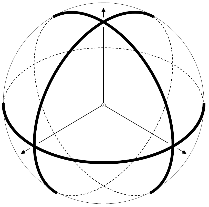
  • [35] V. Voroninski, A comparison between the PhaseLift and PhaseCut algorithms, Available online: http://math.berkeley.edu/~vladv/PhaseCutProofs.pdf
  • [36] V. Voroninski, Phase retrieval from quadratic unitary measurements and implications for Wright’s conjecture, Available online: http://math.berkeley.edu/~vladv/UnitaryCase.pdf
  • [37] I. Waldspurger, A. d’Aspremont, S. Mallat, Phase recovery, MaxCut and complex semidefinite programming, Available online: arXiv:1206.0102
  • [38] A. Walther, The question of phase retrieval in optics, Opt. Acta 10 (1963) 41–49.