跳到论文正文
W Papers独立论文阅读器 arXiv:1307.6839 论文正文 计算阅读时间 · 0%
引用这篇论文根据当前论文元数据生成,正式投稿前建议核对。


License: arXiv.org perpetual non-exclusive license
arXiv:1307.6839v4 [quant-ph] 18 Dec 2014

Bloch sphere colourings and Bell inequalities

Adrian Kent Affiliation: Centre for Quantum Information and Foundations, DAMTP, Centre for Mathematical Sciences, University of Cambridge, Wilberforce Road, Cambridge, CB3 0WA, United Kingdom Affiliation: Perimeter Institute for Theoretical Physics, 31 Caroline Street North, Waterloo, Ontario, Canada N2L 2Y5    Damián Pitalúa-García Affiliation: Centre for Quantum Information and Foundations, DAMTP, Centre for Mathematical Sciences, University of Cambridge, Wilberforce Road, Cambridge, CB3 0WA, United Kingdom
Abstract

We consider the quantum and local hidden variable (LHV) correlations obtained by measuring a pair of qubits by projections defined by randomly chosen axes separated by an angle θ\theta. LHVs predict binary colourings of the Bloch sphere with antipodal points oppositely coloured. We prove Bell inequalities separating the LHV predictions from the singlet quantum correlations for θ∈(0,π3)\theta\in\bigl(0,\frac{\pi}{3}\bigr). We raise and explore the hypothesis that, for a continuous range of θ>0\theta>0, the maximum LHV anticorrelation is obtained by assigning to each qubit a colouring with one hemisphere black and the other white.

I Introduction

According to quantum theory, space-like separated experiments performed on entangled particles can produce outcomes whose correlations violate Bell inequalities [1] that would be satisfied if the experiments could be described by local hidden variable theories (LHVTs). Many experiments have tested the quantum prediction of nonlocal causality (e.g. [2, 3, 4, *GZ99, 6, 7, 8, 9]). The observed violations of Bell inequalities are consistent with quantum theory. They refute LHVTs with overwhelmingly high degrees of confidence, modulo some known loopholes that arise from the difficulty in carrying out theoretically ideal experiments – most notably the locality loophole (closed in [2, 3, 4, 5]), the detection efficiency loophole ([10], closed in [6, 7, 9]) and the collapse locality loophole ([11], addressed in [8], though not fully closed).

Typically, Bell experiments test the CHSH inequality [12] in an EPR-Bohm experiment [13, 14] in which two entangled particles are sent to different experimental setups at different locations. One setup is controlled by Alice, who performs one of two possible measurements A∈{0,1}A\in\{0,1\}; the other by Bob, who similarly performs B∈{0,1}B\in\{0,1\}. Alice’s and Bob’s outcomes aa and bb are assigned numerical values a,b∈{1,−1}a,b\in\{1,-1\}, corresponding to ‘spin up’ or ‘spin down’ for spin measurements about given axes on spin-12\frac{1}{2} particles. The experiments must be completed at space-like separated regions. The experiment is repeated many times, ideally under identical experimental conditions. We define the correlation C⁡(A,B)C(A,B) as the average value of the product of Alice’s and Bob’s outcomes in experiments where measurements AA and BB are chosen.

According to deterministic LHVTs, the outcomes aa, bb are determined respectively by the measurement choices AA, BB and by hidden variables λ\lambda shared by both particles. Thus, a=a⁡(A,λ),b=b⁡(B,λ)a=a(A,\lambda),b=b(B,\lambda). An LHVT also assigns a probability distribution ρ⁡(λ)\rho(\lambda), independent of AA and BB, to the hidden variables, satisfying ρ⁡(λ)≥0\rho(\lambda)\geq 0 and ∫Λd​λ​ρ​(λ)=1\int_{\Lambda}d\lambda\rho(\lambda)=1, where Λ\Lambda is the sample space of hidden variables. Probabilistic LHVTs can be described by the same equations, extending the definitions of λ\lambda and ρ\rho to allow for probabilistic measurement outcomes; we can thus focus on deterministic LHVTs without loss of generality. An LHVT predicts C⁡(A,B)=∫Λd​λ​ρ​(λ)​a​(A,λ)​b​(B,λ)C(A,B)=\int_{\Lambda}d\lambda\rho(\lambda)a(A,\lambda)b(B,\lambda). Such correlations satisfy the CHSH inequality [12]: I2=|C⁡(0,0)+C⁡(1,1)+C⁡(1,0)−C⁡(0,1)|≤2.I_{2}=\bigl\lvert C(0,0)+C(1,1)+C(1,0)-C(0,1)\bigr\rvert\leq 2\,.

Consider for definiteness the EPR-Bohm experiment performed on spin-12\frac{1}{2} particles in the singlet state |Ψ−⟩=12(|↑⟩|↓⟩−|↓⟩|↑⟩)\lvert\Psi^{-}\rangle=\frac{1}{\sqrt{2}}\bigl(\lvert\uparrow\rangle\lvert\downarrow\rangle-\lvert\downarrow\rangle\lvert\uparrow\rangle\bigr). Alice and Bob measure their particle spin projection along the directions a→A\vec{a}_{A} and b→B\vec{b}_{B}, respectively. As before, Alice and Bob choose a measurement from a set of two elements, that is, A,B∈{0,1}A,B\in\{0,1\}. In general, the vectors a→A\vec{a}_{A} and b→B\vec{b}_{B} can point along any direction in three-dimensional Euclidean space, and the sets of their possible values define Bloch spheres 𝕊2\mathbb{S}^{2}. The correlation predicted by quantum theory is Q⁡(θ)=−cos⁡θQ(\theta)=-\cos\theta, where cos⁡θ=a→A⋅b→B\cos\theta=\vec{a}_{A}\cdot\vec{b}_{B}. Sets of measurement axes can be found for which the quantum correlations violate the CHSH inequality, I2QM>2I_{2}^{\text{QM}}>2, up to the Cirel’son [15] bound I2QM≤2​2I_{2}^{\text{QM}}\leq 2\sqrt{2}.

When Alice’s and Bob’s measurement choices belong to a set of NN possible elements, the correlations predicted by LHVTs satisfy the Braunstein-Caves inequality [16]:

IN=|∑k=0N−1C⁡(k,k)+∑k=0N−2C⁡(k+1,k)−C⁡(0,N−1)|≤2​N−2.I_{N}=\Biggl\lvert\sum_{k=0}^{N-1}\!\!C(k,k)+\sum_{k=0}^{N-2}\!\!C(k+1,k)-C(0,N-1)\Biggr\rvert\leq 2N-2. (1)

The CHSH inequality is a special case of the Braunstein-Caves inequality with N=2N=2. We are interested here in exploring Bell inequalities that generalize the CHSH and Braunstein-Caves inequalities, in the following sense. Instead of restricting Alice’s and Bob’s measurement choices to a finite set, we allow them to choose any spin measurement axes, a→\vec{a} and b→\vec{b}. However, we constrain these axes to be separated by a fixed angle θ\theta, so cos⁡θ=a→⋅b→\cos\theta=\vec{a}\cdot\vec{b}. The maximal violation of the Braunstein-Caves inequality by quantum correlations, given by INQM=2​N​cos⁡(π2​N)I_{N}^{\text{QM}}=2N\cos\bigl(\frac{\pi}{2N}\bigr) [17], arises for fixed sets of pairs of axis choices that satisfy this constraint with θ=π2​N\theta=\frac{\pi}{2N}. We consider experiments where pairs of axes separated by θ\theta are chosen randomly and where θ\theta is unrestricted. Our work contributes to understanding how to quantify quantum nonlocality, by studying a natural class of Bell inequalities that has not previously been considered. As well as proving new inequalities, our work raises new questions and suggests new techniques that we hope will be developed further.

Another more practical motivation is to explore simple Bell tests that might allow quantum theory and LHVT to be distinguished somewhat more efficiently, particularly in the adversarial context of quantum cryptography. Here an eavesdropper and/or malicious device manufacturer may be trying to spoof the correlations of a singlet using locally held or generated information. Of course, given sufficient guarantees about the devices involved, modulo the loopholes mentioned above, and with sufficiently many runs, any Bell test can expose such spoofing. However, in practical situations in which the number of possible tests is limited, users would like to ensure that such eavesdropping attacks can be detected as efficiently as possible. Standard CHSH tests simplify the eavesdropper’s problem, by informing her in advance that she need only generate outcomes for a small set of possible measurements. By comparison, tests involving randomly chosen axes give the eavesdropper no such information 11 1 One possibility here is for Alice and Bob to fix in advance the value of θ\theta and a list of random pairs of axes separated by θ\theta. Another would be to make random independent choices and then generate plots of the correlations as a function of θ\theta. This second type of test would be generated automatically by quantum key distribution schemes that require Alice and Bob to make completely random measurements on each qubit (e.g. [34]).. A first step towards understanding Alice’s and Bob’s optimal test strategy in such contexts is to identify the full range of Bell inequalities available.

II Bloch sphere colourings and correlation functions

We explore LHVTs in which Alice’s and Bob’s spin measurement results are given by a⁡(a→,λ)a(\vec{a},\lambda) and b⁡(b→,λ)b\bigl(\vec{b},\lambda\bigr), respectively; where λ\lambda is a local hidden variable common to both particles. For fixed λ\lambda, we can describe the functions aa and bb by two binary (black and white) colourings of spheres, associated with aa and bb, respectively, where black (white) represents the outcome ‘1’ (‘-1’). Different sphere colourings are associated with different values of λ\lambda. To look at specific cases, we drop the λ\lambda-dependence and include a label xx that indicates a particular pair of colouring functions ax​(a→)a_{x}(\vec{a}) and bx​(b→)b_{x}(\vec{b}\!~).

Measuring spin along a→\vec{a} with outcome 1​(−1)1~(-1) is equivalent to measuring spin along −a→-\vec{a} with outcome −1​(1)-1~(1). The colouring functions aa and bb defining any LHVT are thus necessarily antipodal functions:

ax​(a→)=−ax​(−a→),bx​(b→)=−bx​(−b→),a_{x}(\vec{a})=-a_{x}(-\vec{a}),\qquad b_{x}\bigl(\vec{b}~\!\bigr)=-b_{x}\bigl(-\vec{b}~\!\bigr), (2)

for all a→,b→∈𝕊2\vec{a},\vec{b}\in\mathbb{S}^{2}.

We notice that the antipodal property arises due to the definition of a dichotomic measurement on the sphere for arbitrary deterministic LHVTs. For an arbitrary probabilistic theory, this property would read

Px(μa,νb|μa→,νb→)=Px(a,b|a→,b→),P_{x}\bigl(\mu a,\nu b|\mu\vec{a},\nu\vec{b}~\!\bigr)=P_{x}\bigl(a,b|\vec{a},\vec{b}~\!\bigr), (3)

where μ,ν,a,b∈{±1}\mu,\nu,a,b\in\{\pm 1\}, a→,b→∈𝕊2\vec{a},\vec{b}\in\mathbb{S}^{2} and the label xx indicates a particular probabilistic theory being considered. Equation (3) holds because a measurement is defined by a pair of opposite axes, a→\vec{a} and −a→-\vec{a}, and inverting their sense corresponds only to relabelling the measurement outcomes.

We define 𝒳\mathcal{X} as the set of all colourings xx satisfying the antipodal property, Eq. (2). For example, a simple colouring of the spheres satisfying the antipodal property is colouring 1, in which, for one sphere, one hemisphere is completely black and the other one is completely white, and the colouring is reversed for the other sphere (see Fig. 1).

The correlation for outcomes of measurements about randomly chosen axes separated by θ\theta for the pair of colouring functions labelled by xx is

Cx​(θ)=18​π2​∫𝕊2d​A​ax​(a→)​∫02​πd​ω​bx​(b→),C_{x}(\theta)=\frac{1}{8\pi^{2}}\int_{\mathbb{S}^{2}}dAa_{x}(\vec{a})\int_{0}^{2\pi}d\omega b_{x}\bigl(\vec{b}\!~\bigr), (4)

where d​AdA is the area element of the sphere corresponding to Alice’s axis a→\vec{a} and ω\omega is an angle in the range [0,2​π][0,2\pi] along the circle described by Bob’s axis b→\vec{b} with an angle θ\theta with respect to a→\vec{a} . A general correlation is of the form C⁡(θ)=∫𝒳d​x​μ​(x)​Cx​(θ)C(\theta)=\int_{\mathcal{X}}dx\mu(x)C_{x}(\theta), where μ⁡(x)\mu(x) is a probability distribution over 𝒳\mathcal{X}.

If all colourings x∈𝒳x\in\mathcal{X} satisfy QρL​(θ)<CL​(θ)≤Cx​(θ)Q_{\rho_{\text{L}}}(\theta)<C^{\text{L}}(\theta)\leq C_{x}(\theta) or Cx​(θ)≤CU​(θ)<QρU​(θ)C_{x}(\theta)\leq C^{\text{U}}(\theta)<Q_{{\rho}_{\text{U}}}(\theta) for quantum correlations QρL​(θ)Q_{\rho_{\text{L}}}(\theta) and QρU​(θ)Q_{{\rho}_{\text{U}}}(\theta) obtained with particular two-qubit states ρU{\rho_{\text{U}}} and ρL{\rho_{\text{L}}}, and some identifiable lower and upper bounds, CL​(θ)C^{\text{L}}(\theta) and CU​(θ)C^{\text{U}}(\theta), respectively, then a general correlation C⁡(θ)C(\theta) must satisfy the same inequalities. Our aim here is to explore this possibility via intuitive arguments and numerical and analytic results. We focus on the case ρL=|Ψ−⟩⟨Ψ−|{\rho_{\text{L}}}=\lvert\Psi^{-}\rangle\langle\Psi^{-}\rvert, for which QρL​(θ)≡Q⁡(θ)=−cos⁡θQ_{\rho_{\text{L}}}(\theta)\equiv Q(\theta)=-\cos\theta, which is the maximum quantum anticorrelation for a given angle θ\theta (see Sec. V for details and related questions). We begin with some suggestive observations.

First, we consider colouring functions x∈𝒳x\in\mathcal{X} for which the probability that Alice and Bob obtain opposite outcomes when they choose the same measurement, averaged uniformly over all measurement choices, is

P⁡(ax=−bx|θ=0)=1−γ.P(a_{x}=-b_{x}|\theta=0)=1-\gamma. (5)

In general, 0≤γ≤10\leq\gamma\leq 1. We first consider small values of γ\gamma and seek Bell inequalities distinguishing quantum correlations for the singlet from classical correlations for which an anticorrelation is observed with probability 1−γ1-\gamma when the same measurement axis is chosen on both sides. Experimentally, we can verify quantum nonlocality using these results if we carry out nonlocality tests that include some frequency of anticorrelation tests about a randomly chosen axis (chosen independently for each test). The anticorrelation tests allow statistical bounds on γ\gamma, which imply statistical tests of nonlocality via the γ\gamma-dependent Bell inequalities.

In the limiting case γ=0\gamma=0, we have

ax​(a→)=−bx​(a→),a_{x}\left(\vec{a}\right)=-b_{x}\left(\vec{a}\right), (6)

for all a→∈𝕊2\vec{a}\in\mathbb{S}^{2}. This case is quite interesting theoretically, in that one might hope to prove stronger results assuming perfect anticorrelation. We describe some numerical explorations of this case below.

Second, for any pair of colourings x∈𝒳x\in\mathcal{X} and θ∈[0,π]\theta\in[0,\pi], we have Cx​(π−θ)=−Cx​(θ)C_{x}(\pi-\theta)=-C_{x}(\theta). This can be seen as follows. For a fixed a→\vec{a}, the circle with angle θ=θ′\theta=\theta^{\prime} around the axis a→\vec{a}, defined by the angle ω\omega in Eq. (4) contains a point b→\vec{b} that is antipodal to a point on the circle with angle θ=π−θ′\theta=\pi-\theta^{\prime} around a→\vec{a}. Since the colouring is antipodal, we have that the value of the integral ∫02​πd​ω​bx​(b→)\int_{0}^{2\pi}d\omega b_{x}\bigl(\vec{b}\!~\bigr) in Eq. (4) for θ=θ′\theta=\theta^{\prime} is the negative of the corresponding integral for θ=π−θ′\theta=\pi-\theta^{\prime}. It follows that Cx​(π−θ′)=−Cx​(θ′)C_{x}(\pi-\theta^{\prime})=-C_{x}(\theta^{\prime}). Therefore, in the rest of this paper, we restrict to consider correlations for the range θ∈[0,π2]\theta\in\bigl[0,\frac{\pi}{2}\bigr], unless otherwise stated. From the previous argument, we have Cx​(π2)=−Cx​(π2)C_{x}\bigl(\frac{\pi}{2}\bigr)=-C_{x}\bigl(\frac{\pi}{2}\bigr), which implies that Cx​(π2)=0C_{x}\bigl(\frac{\pi}{2}\bigr)=0. We also have that Cx​(0)=1−2​P​(ax=−bx|θ=0)C_{x}(0)=1-2P(a_{x}=-b_{x}|\theta=0), so the LHVTs we consider give Cx​(0)=−1+2​γC_{x}(0)=-1+2\gamma. The LHV correlations given by Eqs. (4) and (5) in the case γ=0\gamma=0 thus coincide with the singlet-state quantum correlations for θ=0\theta=0 and θ=π2\theta=\frac{\pi}{2}, where Q⁡(0)=Cx​(0)=−1Q(0)=C_{x}(0)=-1 and Q⁡(π2)=Cx​(π2)=0Q\bigl(\frac{\pi}{2}\bigr)=C_{x}\bigl(\frac{\pi}{2}\bigr)=0.

Third, consider colouring 1, defined above. We have C1​(θ)=−(1−2​θπ)C_{1}(\theta)=-\bigl(1-\frac{2\theta}{\pi}\bigr), for θ∈[0,π2]\theta\in\bigl[0,\frac{\pi}{2}\bigr]. This is easily seen as follows. For any two different points on the spheres defining colouring 1, a→\vec{a} in one sphere and b→\vec{b} in the oppositely coloured one, an arc of angle π\pi of the great circle passing through a→\vec{a} and b→\vec{b} is completely black and the other arc of angle π\pi is completely white. Thus, given that the pair of vectors a→\vec{a} and b→\vec{b} are chosen randomly, subject to the constraint of angle separation θ\theta, the probability that both a→\vec{a} and b→\vec{b} are in oppositely coloured regions is P⁡(a1=−b1|θ)=π−θπ=1−θπP(a_{1}=-b_{1}|\theta)=\frac{\pi-\theta}{\pi}=1-\frac{\theta}{\pi}. Thus, the correlation for colouring 1 is C1​(θ)=1−2​P​(a1=−b1|θ)=−1+2​θπC_{1}(\theta)=1-2P(a_{1}=-b_{1}|\theta)=-1+\frac{2\theta}{\pi}. That is, C1​(θ)C_{1}(\theta) linearly interpolates between the values at C1​(0)=−1C_{1}(0)=-1, which is common to all colourings with γ=0\gamma=0, and C1​(π2)=0C_{1}\bigl(\frac{\pi}{2}\bigr)=0, which is common to all colourings, and we have 0>C1​(θ)>Q⁡(θ)0>C_{1}(\theta)>Q(\theta) for θ∈(0,π2)\theta\in\bigl(0,\frac{\pi}{2}\bigr).

Then, in the following section we present some lemmas and a theorem.

III Hemispherical Colouring Maximality Hypotheses

In this section, we motivate two hemispherical colouring maximality hypotheses. These make precise the intuition that, for a continuous range of θ>0\theta>0, the maximum LHV anticorrelation is obtained by colouring 11.

We first consider the following lemmas, whose proofs are given in Appendix A.

Lemma 1.

For any colouring x∈𝒳x\in\mathcal{X} satisfying Eq. (5) and any θ∈(0,2​π3]\theta\in\bigl(0,\frac{2\pi}{3}\bigr], we have −1+23​γ≤Cx​(θ)≤13+23​γ-1+\frac{2}{3}\gamma\leq C_{x}(\theta)\leq\frac{1}{3}+\frac{2}{3}\gamma.

Remark 1.

Unsurprisingly, since small γ\gamma implies near-perfect anticorrelation at θ=0\theta=0, we see that for θ∈(0,2​π3]\theta\in\bigl(0,\frac{2\pi}{3}\bigr] and γ\gamma small there are no colourings with very strong correlations. However, strong anticorrelations are possible for small θ\theta. We are interested in bounding these.

Lemma 2.

For any colouring x∈𝒳x\in\mathcal{X} satisfying Eq. (5), any integer N>2N>2 and any θ∈[πN,πN−1)\theta\in\bigl[\frac{\pi}{N},\frac{\pi}{N-1}\bigr), we have Cx​(θ)≥C1​(πN)−2​γC_{x}(\theta)\geq C_{1}\bigl(\frac{\pi}{N}\bigr)-2\gamma.

Remark 2.

In other words, for small θ\theta, C1​(θ)C_{1}(\theta) is very close to the maximal possible anticorrelation for LHVTs when γ≪θ\gamma\ll\theta.

Geometric intuitions also suggest bounds on Cx​(θ)C_{x}(\theta) that are maximised by colouring 11 for small θ\theta. Consider simple colourings, in which a set of (not necessarily connected) piecewise differentiable curves of finite total length separate black and white regions. (Points lying on these curves may have either colour.) Intuition suggests that, for small θ\theta and simple colourings with γ=0\gamma=0, the quantity 1+Cx​(θ)1+C_{x}(\theta), which measures the deviation from pure anticorrelation, should be bounded by a quantity roughly proportional to the length of the boundary between the black and white areas of the sphere colouring x∈𝒳x\in\mathcal{X}. Since colouring 11 has the smallest such boundary (the equator), this might suggest that Cx​(θ)≥C1​(θ),C_{x}(\theta)\geq C_{1}(\theta)\,, for small θ\theta and for all simple colourings x∈𝒳x\in\mathcal{X} with γ=0\gamma=0. Intuition also suggests that any non-simple colouring will produce less anticorrelation than the optimal simple colouring, because regions in which black and white colours alternate with arbitrarily small separation tend to wash out anticorrelation. These intuitive arguments are clearly not rigorous as currently formulated. For example, they ignore the possibility of sequences of colourings Ci​(θ)C_{i}(\theta) and angles θi→0\theta_{i}\rightarrow 0 such that Ci​(θi)<C1​(θi)C_{i}(\theta_{i})<C_{1}(\theta_{i}), while limθ→0(Ci​(θ)−C1​(θ))>0\lim_{\theta\rightarrow 0}(C_{i}(\theta)-C_{1}(\theta))>0 for all ii (see [19] for an extended discussion). Still, they are suggestive, at least in generating hypotheses to be investigated.

These various observations motivate us to explore what we call the weak hemispherical colouring maximality hypothesis (WHCMH).

The WHCMH.

There exists an angle θmaxw∈(0,π2)\theta_{\text{max}}^{\text{w}}\in\bigl(0,\frac{\pi}{2}\bigr) such that for every colouring x∈𝒳x\in\mathcal{X} with γ=0\gamma=0 and every angle θ∈[0,θmaxw]\theta\in[0,\theta_{\text{max}}^{\text{w}}], Cx​(θ)≥C1​(θ)C_{x}(\theta)\geq C_{1}(\theta).

The WHCMH considers models with perfect anticorrelation for θ=0\theta=0, because we are interested in distinguishing LHV models from the quantum singlet state, which produces perfect anticorrelations for θ=0\theta=0. Of course, there is a symmetry in the space of LHV models given by exchanging the colours of one qubit’s sphere, which maps γ→1−γ\gamma\rightarrow 1-\gamma and Cx​(θ)→−Cx​(θ)C_{x}(\theta)\rightarrow-C_{x}(\theta). The WHCMH thus also implies that Cx​(θ)≤−C1​(θ)C_{x}(\theta)\leq-C_{1}(\theta) for all colourings x∈𝒳x\in\mathcal{X} with γ=1\gamma=1.

It is also interesting to investigate stronger versions of the WHCMH and related questions. For instance, is it the case that for every angle θ∈(θmaxw,π2)\theta\in\bigl(\theta_{\text{max}}^{\text{w}},\frac{\pi}{2}\bigr) there exists a colouring x′∈𝒳x^{\prime}\in\mathcal{X} with γ=0\gamma=0 such that Cx′​(θ)<C1​(θ)C_{x^{\prime}}(\theta)<C_{1}(\theta)? Further, does this hypothesis still hold true (not necessarily for the same θmaxw\theta_{\text{max}}^{\text{w}}) if we consider general local hidden variable models corresponding to independently chosen colourings for the two qubits, not constrained by any choice of the correlation parameter γ\gamma?

The following theorem and lemmas, whose proofs are presented in Appendix A, give some relevant bounds.

Theorem 1.

For any colouring x∈𝒳x\in\mathcal{X}, any integer N≥2N\geq 2 and any θ∈[π2​N,π2​(N−1))\theta\in\bigl[\frac{\pi}{2N},\frac{\pi}{2(N-1)}\bigr), we have C1​(π2​N)≤Cx​(θ)≤−C1​(π2​N)C_{1}\bigl(\frac{\pi}{2N}\bigr)\leq C_{x}(\theta)\leq-C_{1}\bigl(\frac{\pi}{2N}\bigr).

Remark 3.

In particular, for small θ\theta, −C1​(θ)-C_{1}(\theta) and C1​(θ)C_{1}(\theta) are very close to the maximal possible correlation and anticorrelation for any LHVT, respectively.

Lemma 3.

If any colouring x∈𝒳x\in\mathcal{X} obeys Cx​(θ)<C1​(θ)​(Cx​(θ)>−C1​(θ))C_{x}(\theta)<C_{1}(\theta)~\Bigl(C_{x}(\theta)>-C_{1}(\theta)\Bigr) for some θ∈(πM+1,πM]\theta\in\bigl(\frac{\pi}{M+1},\frac{\pi}{M}\bigr] and an integer M≥2M\geq 2 then there are angles θj≡πM+1−j−θ\theta_{j}\equiv\frac{\pi}{M+1-j}-\theta with j=1,2,…,M−1j=1,2,\ldots,M-1, which satisfy 0≤θj<θ0\leq\theta_{j}<\theta if j<M2+1j<\frac{M}{2}+1, and π2>θj>θ\frac{\pi}{2}>\theta_{j}>\theta if j≥M2+1j\geq\frac{M}{2}+1, such that Cx​(θj)>C1​(θj)​(Cx​(θj)<−C1​(θj))C_{x}(\theta_{j})>C_{1}(\theta_{j})~\Bigl(C_{x}(\theta_{j})<-C_{1}(\theta_{j})\Bigr).

Remark 4.

In this sense (at least), the anticorrelations defined by C1C_{1} and the correlations defined by −C1-C_{1} cannot be dominated by any other colourings.

Lemma 4.

For any colouring x∈𝒳x\in\mathcal{X} and any θ∈(0,π3)\theta\in\bigl(0,\frac{\pi}{3}\bigr), we have Q⁡(θ)<Cx​(θ)<−Q⁡(θ)Q(\theta)<C_{x}(\theta)<-Q(\theta).

Remark 5.

This inequality separates all possible LHV correlations Cx​(θ)C_{x}(\theta) from the singlet-state quantum correlations Q⁡(θ)Q(\theta) for all θ∈(0,π3)\theta\in\bigl(0,\frac{\pi}{3}\bigr).

The previous observations motivate the strong hemispherical colouring maximality hypothesis (SHCMH).

The SHCMH.

There exists an angle θmaxs∈(0,π2)\theta_{\text{max}}^{\text{s}}\in\bigl(0,\frac{\pi}{2}\bigr) such that for every colouring x∈𝒳x\in\mathcal{X} and every angle θ∈[0,θmaxs]\theta\in[0,\theta_{\text{max}}^{\text{s}}], C1​(θ)≤Cx​(θ)≤−C1​(θ)C_{1}(\theta)\leq C_{x}(\theta)\leq-C_{1}(\theta).

Note that the SHCMH applies to all colourings, without any assumption of perfect anticorrelation for θ=0\theta=0. If the SHCMH is true then so is the WHCMH. In this case, we have that θmaxs≤θmaxw\theta_{\text{max}}^{\text{s}}\leq\theta_{\text{max}}^{\text{w}}. Thus, an upper bound on θmaxw\theta_{\text{max}}^{\text{w}} implies an upper bound on θmaxs\theta_{\text{max}}^{\text{s}}.

IV Numerical results

We investigated the WHCMH numerically by computing the correlation Cx​(θ)C_{x}(\theta) for various colouring functions that satisfy the antipodal property, Eq. (2), the condition (6), and that have azimuthal symmetry (see Fig. 1). Details of our numerical work are given in Appendix C. Our numerical results are consistent with the WHCMH for θmaxw≤0.386​π\theta_{\text{max}}^{\text{w}}\leq 0.386\pi, and with the SHCMH for θmaxs≤0.375​π\theta_{\text{max}}^{\text{s}}\leq 0.375\pi, but do not give strong evidence for these values. Nor do the numerical results, per se, constitute compelling evidence for the WHCMH and SHCMH, although they confirm that the underlying intuitions hold for some simple colourings.

We note that the slightly improved bound θmaxs≤0.345​π\theta_{\text{max}}^{\text{s}}\leq 0.345\pi was obtained in [19]. Further details are given in Appendix C.

Refer to caption
Figure 1: Some antipodal colouring functions axa_{x} on the sphere, see Appendix C for definitions. Their correlations Cx​(θ)C_{x}(\theta), computed from Eq. (4), subject to the constraint (6), are plotted in Appendix C.

V Related questions for exploration

An interesting related question is, for an arbitrary two-qubit state ρ\rho and qubit projective measurements performed by Alice and Bob corresponding to random Bloch vectors separated by an angle θ\theta, what are the maximum values of the quantum correlations and anticorrelations Qρ​(θ)Q_{\rho}(\theta), and which states achieve them? We show that the maximum quantum anticorrelations and correlations are Qρ​(θ)=−cos⁡θQ_{\rho}(\theta)=-\cos\theta, achieved by the singlet state ρ=|Ψ−⟩⟨Ψ−|\rho=\lvert\Psi^{-}\rangle\langle\Psi^{-}\rvert, and Qρ​(θ)=13​cos⁡θQ_{\rho}(\theta)=\frac{1}{3}\cos\theta, achieved by the other Bell states, ρ=|Φ±⟩⟨Φ±|\rho=\lvert\Phi^{\pm}\rangle\langle\Phi^{\pm}\rvert and ρ=|Ψ+⟩⟨Ψ+|\rho=\lvert\Psi^{+}\rangle\langle\Psi^{+}\rvert, respectively. This result follows because, as we show in Appendix B, we have

−cos⁡θ≤Qρ​(θ)≤13​cos⁡θ.-\cos{\theta}\leq Q_{\rho}(\theta)\leq\frac{1}{3}\cos{\theta}. (7)

Another related question that we do not explore further here is, for a fixed given angle θ\theta separating Alice’s and Bob’s measurement axes, what are the maximum correlations and anticorrelations, if in addition to the two-qubit state ρ\rho, Alice and Bob have other resources? For example, Alice and Bob could have an arbitrary entangled state on which they perform arbitrary local quantum operations and measurements. In a different scenario, Alice and Bob could have some amount of classical or quantum communication. Another possibility is for Alice and Bob to share arbitrary no-signalling resources, not necessarily quantum, with no communication allowed. Different variations of the task described above with continuous parameters can be investigated.

One might ask what constraints the no-signalling principle places on the correlations and anticorrelations. A generalised PR-box [20] gives the correlation C⁡(θ)=sign⁡(π/2−θ)C(\theta)={\rm sign}(\pi/2-\theta), which in one natural sense defines the strongest correlations consistent with Eq. (3). Another relevant observation is that the antipodal property (3), expressed in the equivalent form C⁡(π−θ)=−C⁡(θ)C(\pi-\theta)=-C(\theta), together with a continuity assumption, implies that quantum nonlocal correlations are not dominated [21]: If a correlation C⁡(θ)C(\theta) produces a violation of the CHSH inequality stronger than the violation given by the singlet-state quantum correlation Q⁡(θ)Q(\theta) for a given set of measurement axes then there exists another set of measurement axes for which C⁡(θ)C(\theta) gives a violation (or none) that is weaker than the violation given by Q⁡(θ)Q(\theta). It would be interesting to clarify further the relationship between measures of nonlocality, including those investigated here, and no-signalling.

Other related questions are given in Appendix B.

VI Discussion

We have explored here what can be learned by carrying out local projective measurements about completely randomly chosen axes, separated by an angle θ\theta, on a pair of qubits. This is not currently a standard way of testing for entanglement or nonlocality, but we have shown that it distinguishes quantum correlations from those predicted by local hidden variables for a wide range of θ\theta. In particular, we find Bell inequalities for θ∈(0,π2)\theta\in\bigl(0,\frac{\pi}{2}\bigr), given by Theorem 1, which separate the singlet-state quantum correlations from all LHV correlations for θ∈(0,π3)\theta\in\bigl(0,\frac{\pi}{3}\bigr).

We have also explored hypotheses that would refine and unify these results further: the weak and strong hemispherical colouring maximality hypotheses. These state that the LHV defined by the simplest spherical colouring, with opposite hemispheres coloured oppositely, maximizes the LHV anticorrelations for a continuous range of θ>0\theta>0, either among LHVs with perfect anticorrelation at θ=0\theta=0 (the weak case) or without any restriction (the strong case).

We should note here that the intuition supporting the WHCMH relates specifically to colourings in two or more dimensions, where there seems no obvious way of constructing colourings that vary over small scales in a way that is regular enough to produce very strong (anti) correlations for small θ\theta.

On the other hand, the one-dimensional analog of the WHCMH – that the strongest anticorrelations for colourings on the circle arise from colouring opposite half-circles oppositely – is easily seen to be false. For nn odd, the colouring a⁡(ϵ)=−b⁡(ϵ)=(−1)⌊n​ϵπ⌋a(\epsilon)=-b(\epsilon)=(-1)^{\lfloor\frac{n\epsilon}{\pi}\rfloor} with ϵ∈[0,2​π]\epsilon\in[0,2\pi] is antipodal and is perfectly anticorrelated for θ=2​πn\theta=\frac{2\pi}{n}.

Although it underlines that the hemispherical colouring hypotheses are non-trivial, this distinction between one and higher dimensions is consistent with what is known about other colouring problems in geometric combinatorics [22, 23]. The intuition that colouring 11 should be optimal, because it solves the isoperimetric problem of finding the coloured region with half the area of the sphere that has the shortest boundary, remains suggestive. Verifying the WHCMH and the SHCMH look at first sight like simple classical problems in geometry and combinatorics that can be stated quite independently of quantum theory. They have many interesting generalisations 22 2 For example, among non-antipodal bipartite colourings of the sphere in which the black region has area A<2​πA<2\pi, which colouring(s) produce maximal correlation? Or, consider a general region RR of volume VV in ℝn\mathbb{R}^{n}, and define pϵ​(R)p_{\epsilon}(R) to be the probability that, given a randomly chosen point x∈Rx\in R, and a randomly chosen point yy such that d⁡(x,y)=ϵd(x,y)=\epsilon, we find that y∈Ry\in R. Do the balls maximize this probability, for any given sufficiently small ϵ\epsilon?. Nonetheless, as far as we are aware, these questions have not been seriously studied by pure mathematicians to date, although some intriguing relatively recent results [22, 23] on colourings in ℝn\mathbb{R}^{n} encourage hope that proof methods could indeed be found. We thus simply state the WHCMH and the SHCMH as interesting and seemingly plausible hypotheses to be investigated further rather than offering them as conjectures, preferring to reserve the latter terms for propositions for which very compelling evidence has been amassed.

We would like to stress what we see as a key insight deserving further exploration, namely that stronger and more general Bell inequalities could in principle be proven by results about continuous colourings, rather than restricting to colourings of discrete sets. While we have focussed on the simplest case of projective measurements of pairs of qubits, this observation of course applies far more generally. We hope our work will stimulate further investigation of the WHCMH and the SHCMH and related colouring problems, which seem very interesting in their own right, and in developing further this intriguing link between pretty and natural questions in geometric combinatorics and measures of quantum nonlocality.

We have considered here the ideal case in which Alice and Bob share a maximally entangled pure state and are able to carry out perfect projective measurements about axes specified with perfect precision. For a range of non-zero θ\theta, our results show a finite separation between the predictions of quantum theory and LHVTs. As is the case for CHSH and other Bell tests, they can thus also be applied (within a certain parameter range) to realistic experiments in which the entangled state is mixed and measurements can only be approximately specified. In particular, they offer new methods for exploring the range of parameters for which the correlations defined by rotationally symmetric Werner states can be distinguished from those of any LHVT [25, 26, 27, 28]. It would be interesting to explore this further.

Finally, but importantly, we would like to note earlier work on related questions. In a pioneering paper, Żukowski [29] considered generalised Bell and GHZ tests for maximally entangled quantum states that involve all possible axis choices, and gave an elegant proof that the quantum correlations can be distinguished from all possible LHVT correlations by a weighted average measure of correlation functions. For the bipartite case, our work investigates the gap between quantum and LHVT correlations at each axis angle separation. This allows one to define infinitely many generalised Bell tests corresponding to different weighted averages of correlation functions. It would be interesting to characterise the space of all such tests and its boundaries.

References [30, 31, 32] investigate inter alia Bell-CHSH experiments in which the axes are initially chosen randomly, and the same axes are used repeatedly throughout a given experimental run. Reference [30] shows that such experiments lead to Bell inequality violations a significant fraction of the time when pairs of random local measurements are chosen. References [31, 32] show that by considering triads of random local measurements, constrained to be mutually unbiased, for which Alice’s axes are not perfectly aligned to Bob’s axes, the violation of a CHSH inequality is guaranteed on a two qubit maximally entangled state. Their scenarios are significantly different from ours. In our scenario, the axes are chosen randomly and independently for each measurement, and (in the ideal case) Alice and Bob have the ability to define their axis choices precisely with respect to the same reference frame. The goals are also different: References [30, 31, 32] show that Bell inequality violation can be demonstrated even when Alice and Bob do not have a shared reference frame; our aim is to establish new Bell inequalities rather than to exploit the power of known inequalities. It would be interesting to explore possible connections, nonetheless.

After completing this work, our attention was also drawn to a related question considered in [33]; see Appendix B for discussion.

Acknowledgements.
We thank Boris Bukh for very helpful discussions and for drawing our attention to Refs. [22, 23]. A.K. was partially supported by a grant from the John Templeton Foundation and by Perimeter Institute for Theoretical Physics. Research at Perimeter Institute is supported by the Government of Canada through Industry Canada and by the Province of Ontario through the Ministry of Research and Innovation. D.P.-G. thanks Tony Short, Boris Groisman and Jonathan Barrett for helpful discussions, and acknowledges financial support from CONACYT México and partial support from Gobierno de Veracruz.

Appendix A Proofs of the theorem and lemmas

A.1 Proof of Lemma 1

From the CHSH inequality,

|C(0,0)+C(1,1)+C(1,0)−C(0,1)|≤2,\bigl\lvert C(0,0)+C(1,1)+C(1,0)-C(0,1)\bigr\rvert\leq 2\,, (8)

in the case in which the measurements A=0A=0, A=1A=1 and B=0B=0 correspond to projections on states with Bloch vectors separated from each other by the same angle θ∈(0,2​π3]\theta\in\bigl(0,\frac{2\pi}{3}\bigr], Bob’s measurement B=1B=1 is the same as Alice’s measurement A=0A=0 and the outcomes are described by LHVTs satisfying (4), we obtain after averaging over random rotations of the Bloch sphere that |3​Cx​(θ)−Cx​(0)|≤2\lvert 3C_{x}(\theta)-C_{x}(0)\rvert\leq 2. Then, the result follows because, as shown in the main text, we have Cx​(0)=−1+2​γC_{x}(0)=-1+2\gamma.∎

A.2 Proof of Lemma 2

From the Braunstein-Caves inequality, Eq. (1), we have that

IN=|∑k=0N−1C⁡(k,k)+∑k=0N−1C⁡(k+1,k)|≤2​N−2,I_{N}=\biggl\lvert\sum_{k=0}^{N-1}C(k,k)+\sum_{k=0}^{N-1}C(k+1,k)\biggr\rvert\leq 2N-2\,, (9)

with the convention that measurement choice NN is measurement choice 00 with reversed outcomes. We consider the case in which Alice’s and Bob’s measurement kk are the same, for k=0,1,…,N−1k=0,1,\ldots,N-1 and N≥2N\geq 2, and their outcomes are described by LHVTs satisfying (4) and (5), which then also satisfy Cx​(0)=−1+2​γC_{x}(0)=-1+2\gamma. If we take measurement kk to be of the projection onto the state |ξk⟩\lvert\xi_{k}\rangle so that the states {|ξk⟩}k=0N−1\{\lvert\xi_{k}\rangle\}_{k=0}^{N-1} are along a great circle on the Bloch sphere with a separation angle θ=πN\theta=\frac{\pi}{N} between |ξk⟩\lvert\xi_{k}\rangle and |ξk+1⟩\lvert\xi_{k+1}\rangle for k=0,1,…,N−2k=0,1,\ldots,N-2, for example |ξk⟩=cos(k​π2​N)|0⟩+sin(k​π2​N)|1⟩\lvert\xi_{k}\rangle=\cos\bigl(\frac{k\pi}{2N}\bigr)\lvert 0\rangle+\sin\bigl(\frac{k\pi}{2N}\bigr)\lvert 1\rangle, and average over random rotations of the Bloch sphere, this gives

|NCx(0)+NCx(θ)|≤2N−2.\bigl\lvert NC_{x}(0)+NC_{x}(\theta)\bigr\rvert\leq 2N-2\,. (10)

Since Cx​(0)=−1+2​γC_{x}(0)=-1+2\gamma, it follows that Cx​(πN)≥−1+2N−2​γ=C1​(πN)−2​γ.C_{x}\bigl(\frac{\pi}{N}\bigr)\geq-1+\frac{2}{N}-2\gamma=C_{1}\bigl(\frac{\pi}{N}\bigr)-2\gamma\,. Similarly, if we take the states {|ξk⟩}k=0N−1\{\lvert\xi_{k}\rangle\}_{k=0}^{N-1} to be along a zigzag path crossing a great circle on the Bloch sphere with a separation angle θ>πN\theta>\frac{\pi}{N} between |ξk⟩\lvert\xi_{k}\rangle and |ξk+1⟩\lvert\xi_{k+1}\rangle for k=0,1,…,N−2k=0,1,\ldots,N-2, in such a way that the angle separation between |ξN−1⟩\lvert\xi_{N-1}\rangle and the state with Bloch vector antiparallel to that one of |ξ0⟩\lvert\xi_{0}\rangle is also θ\theta (see Fig. 2), we obtain after averaging over random rotations of the Bloch sphere that Cx​(θ)≥−1+2N−2​γ=C1​(πN)−2​γC_{x}(\theta)\geq-1+\frac{2}{N}-2\gamma=C_{1}\bigl(\frac{\pi}{N}\bigr)-2\gamma.∎

Refer to caption
Figure 2: Diagram of the measurements performed by Alice and Bob that are used in the proof of Lemma 2. Alice’s and Bob’s measurements kk are the same, for k=0,1,…,N−1k=0,1,\ldots,N-1 and N≥2N\geq 2; these are projections onto the states |ξk⟩\lvert\xi_{k}\rangle and correspond to points in the Bloch sphere with label kk. These points form a zigzag path crossing the dashed great circle. The state |ξN⟩\lvert\xi_{N}\rangle is antipodal to |ξ0⟩\lvert\xi_{0}\rangle and represents the measurement k=0k=0 with reversed outcomes. The solid lines represent arcs of great circles with the same angle θ>πN\theta>\frac{\pi}{N} that connect adjacent points. If θ=πN\theta=\frac{\pi}{N}, all these points are on the same great circle.

A.3 Proof of Theorem 1

Consider the Braunstein-Caves inequality, Eq. (1), in the case in which Alice’s and Bob’s measurement outcomes are described by LHVTs satisfying (4). Let Alice’s and Bob’s measurements kk correspond to the projections onto the states |ξk⟩\lvert\xi_{k}\rangle and |χk⟩\lvert\chi_{k}\rangle, respectively, for k=0,1,…,N−1k=0,1,\ldots,N-1 and N≥2N\geq 2. Let the angle along the great circle in the Bloch sphere passing through the states |ξk⟩\lvert\xi_{k}\rangle and |χk⟩\lvert\chi_{k}\rangle be θ\theta, for k=0,1,…,N−1k=0,1,\ldots,N-1. Similarly, let the angle along the great circle passing through |χk⟩\lvert\chi_{k}\rangle and |ξk+1⟩\lvert\xi_{k+1}\rangle be θ\theta for k=0,1,…,N−1k=0,1,\ldots,N-1, with the convention that the state |ξN⟩\lvert\xi_{N}\rangle has Bloch vector antiparallel to that one of |ξ0⟩\lvert\xi_{0}\rangle. If θ=π2​N\theta=\frac{\pi}{2N}, all these states are on the same great circle beginning at |ξ0⟩\lvert\xi_{0}\rangle and ending at |ξN⟩\lvert\xi_{N}\rangle. If θ>π2​N\theta>\frac{\pi}{2N}, the states can be accommodated on a zigzag path crossing the great circle that goes from |ξ0⟩\lvert\xi_{0}\rangle to |ξN⟩\lvert\xi_{N}\rangle (see Fig. 3). Thus, from the Braunstein-Caves inequality, after averaging over random rotations of the Bloch sphere, we have C1​(π2​N)=−1+1N≤Cx​(θ)≤1−1N=−C1​(π2​N)C_{1}\bigl(\frac{\pi}{2N}\bigr)=-1+\frac{1}{N}\leq C_{x}(\theta)\leq 1-\frac{1}{N}=-C_{1}\bigl(\frac{\pi}{2N}\bigr), for θ≥π2​N\theta\geq\frac{\pi}{2N}.∎

Refer to caption
Figure 3: Diagram of the measurements performed by Alice and Bob that are used in the proof of Theorem 1. Alice’s and Bob’s measurements AA and BB are projections onto the state |ξA⟩\lvert\xi_{A}\rangle and |χB⟩\lvert\chi_{B}\rangle and correspond to points in the Bloch sphere with labels AA and BB, respectively, for A,B∈{0,1,…,N−1}A,B\in\{0,1,\ldots,N-1\} and N≥2N\geq 2. These points form a zigzag path crossing the dashed great circle. The state |ξN⟩\lvert\xi_{N}\rangle is antipodal to |ξ0⟩\lvert\xi_{0}\rangle and represents Alice’s measurement A=0A=0 with reversed outcomes. The solid lines represent arcs of great circles with the same angle θ>π2​N\theta>\frac{\pi}{2N} that connect adjacent points. If θ=π2​N\theta=\frac{\pi}{2N}, all these points are on the same great circle.

A.4 Proof of Lemma 3

Consider a colouring x∈𝒳x\in\mathcal{X} and an angle θ∈(πM+1,πM]\theta\in\bigl(\frac{\pi}{M+1},\frac{\pi}{M}\bigr] for an integer M≥2M\geq 2 such that Cx​(θ)<C1​(θ)C_{x}(\theta)<C_{1}(\theta) or Cx​(θ)>−C1​(θ)C_{x}(\theta)>-C_{1}(\theta). From Theorem 1 and the fact that Cx​(π2)=C1​(π2)=0C_{x}\bigl(\frac{\pi}{2}\bigr)=C_{1}\bigl(\frac{\pi}{2}\bigr)=0, it must be that θ≠πM\theta\neq\frac{\pi}{M} if MM is even. We define the angles θj≡πM+1−j−θ\theta_{j}\equiv\frac{\pi}{M+1-j}-\theta with j=1,2,…,M−1j=1,2,\ldots,M-1. Considering the cases MM even and MM odd, and using that θ≠πM\theta\neq\frac{\pi}{M} if MM is even, it is straightforward to obtain that 0≤θj<θ0\leq\theta_{j}<\theta if j<M2+1j<\frac{M}{2}+1 and π2>θj>θ\frac{\pi}{2}>\theta_{j}>\theta if j≥M2+1j\geq\frac{M}{2}+1. Now consider the Braunstein-Caves inequality, Eq. (1), in the case in which Alice’s and Bob’s measurement outcomes are described by LHVTs satisfying (4). Let Alice’s and Bob’s measurements kk correspond to the projections onto the states |ξk⟩\lvert\xi_{k}\rangle and |χk⟩\lvert\chi_{k}\rangle, respectively, for k=0,1,…,N−1k=0,1,\ldots,N-1 and N≡M+1−jN\equiv M+1-j. Since 1≤j≤M−11\leq j\leq M-1, we have 2≤N≤M2\leq N\leq M. Let all these states be on the great circle in the Bloch sphere that passes through the states |ξ0⟩\lvert\xi_{0}\rangle and |ξN⟩\lvert\xi_{N}\rangle, with the convention that the state |ξN⟩\lvert\xi_{N}\rangle has Bloch vector antiparallel to that one of |ξ0⟩\lvert\xi_{0}\rangle. Let the angles between |ξk⟩\lvert\xi_{k}\rangle and |χk⟩\lvert\chi_{k}\rangle, and between |χk⟩\lvert\chi_{k}\rangle and |ξk+1⟩\lvert\xi_{k+1}\rangle along this great circle be θ\theta and θj\theta_{j}, respectively. For example, |ξk⟩=cos(k​π2​N)|0⟩+sin(k​π2​N)|1⟩\lvert\xi_{k}\rangle=\cos\bigl(\frac{k\pi}{2N}\bigr)\lvert 0\rangle+\sin\bigl(\frac{k\pi}{2N}\bigr)\lvert 1\rangle and |χk⟩=cos(k​π2​N+θ2)|0⟩+sin(k​π2​N+θ2)|1⟩\lvert\chi_{k}\rangle=\cos\bigl(\frac{k\pi}{2N}+\frac{\theta}{2}\bigr)\lvert 0\rangle+\sin\bigl(\frac{k\pi}{2N}+\frac{\theta}{2}\bigr)\lvert 1\rangle, for k=0,1,…,N−1k=0,1,\ldots,N-1. From the Braunstein-Caves inequality, after averaging over random rotations of the Bloch sphere, we obtain −1+1N≤12​(Cx​(θ)+Cx​(θj))≤1−1N-1+\frac{1}{N}\leq\frac{1}{2}\bigl(C_{x}(\theta)+C_{x}(\theta_{j})\bigr)\leq 1-\frac{1}{N}. Since the average angle θ¯j≡12​(θ+θj)\bar{\theta}_{j}\equiv\frac{1}{2}(\theta+\theta_{j}) satisfies θ¯j=π2​(M+1−j)=π2​N\bar{\theta}_{j}=\frac{\pi}{2(M+1-j)}=\frac{\pi}{2N} and C1​(π2​N)=−1+1NC_{1}(\frac{\pi}{2N})=-1+\frac{1}{N}, we have C1​(θ¯j)≤12​(Cx​(θ)+Cx​(θj))≤−C1​(θ¯j)C_{1}\bigl(\bar{\theta}_{j}\bigr)\leq\frac{1}{2}\bigl(C_{x}(\theta)+C_{x}(\theta_{j})\bigr)\leq-C_{1}\bigl(\bar{\theta}_{j}\bigr). Since C1​(θ)C_{1}(\theta) is a linear function of θ\theta, it follows that Cx​(θj)>C1​(θj)C_{x}(\theta_{j})>C_{1}(\theta_{j}) if Cx​(θ)<C1​(θ)C_{x}(\theta)<C_{1}(\theta). Similarly, Cx​(θj)<−C1​(θj)C_{x}(\theta_{j})<-C_{1}(\theta_{j}) if Cx​(θ)>−C1​(θ)C_{x}(\theta)>-C_{1}(\theta).∎

A.5 Proof of Lemma 4

Let x∈𝒳x\in\mathcal{X} be any colouring and θ∈(0,π3)\theta\in\bigl(0,\frac{\pi}{3}\bigr). We first consider the case θ∈[π4,π3)\theta\in\bigl[\frac{\pi}{4},\frac{\pi}{3}\bigr). From Theorem 1, we have C1​(π4)≤Cx​(θ)≤−C1​(π4)C_{1}\bigl(\frac{\pi}{4})\leq C_{x}(\theta)\leq-C_{1}\bigl(\frac{\pi}{4}). The quantum correlation for the singlet state is Q⁡(θ)=−cos⁡θQ(\theta)=-\cos{\theta}. Since Q⁡(θ)Q(\theta) is a strictly increasing function of θ\theta, we have Q⁡(θ)<Q⁡(π3)=−12=C1​(π4)Q(\theta)<Q\bigl(\frac{\pi}{3}\bigr)=-\frac{1}{2}=C_{1}\bigl(\frac{\pi}{4}\bigr) for θ<π3\theta<\frac{\pi}{3}. Therefore, Q⁡(θ)<Cx​(θ)<−Q⁡(θ)Q(\theta)<C_{x}(\theta)<-Q(\theta) for θ∈[π4,π3)\theta\in\bigl[\frac{\pi}{4},\frac{\pi}{3}\bigr). Similarly, it is easy to see that Q⁡(θ)<Cx​(θ)<−Q⁡(θ)Q(\theta)<C_{x}(\theta)<-Q(\theta) for θ∈[π6,π4)\theta\in\bigl[\frac{\pi}{6},\frac{\pi}{4}\bigr). Now we consider the case θ∈(0,π6)\theta\in\bigl(0,\frac{\pi}{6}\bigr). We define N=⌈π2​θ⌉N=\lceil\frac{\pi}{2\theta}\rceil. It follows that θ∈[π2​N,π2​(N−1))\theta\in\bigl[\frac{\pi}{2N},\frac{\pi}{2(N-1)}\bigr) for an integer N≥4N\geq 4. From Theorem 1, we have −1+1N=C1​(π2​N)≤Cx​(θ)≤−C1​(π2​N)=1−1N-1+\frac{1}{N}=C_{1}\bigl(\frac{\pi}{2N}\bigr)\leq C_{x}(\theta)\leq-C_{1}\bigl(\frac{\pi}{2N}\bigr)=1-\frac{1}{N}. From the Taylor series Q⁡(θ)=−1+θ22−θ44!+θ66!−⋯Q(\theta)=-1+\frac{\theta^{2}}{2}-\frac{\theta^{4}}{4!}+\frac{\theta^{6}}{6!}-\cdots, it is easy to see that Q⁡(θ)<−1+θ22Q(\theta)<-1+\frac{\theta^{2}}{2} for 0<θ<300<\theta<\sqrt{30}. Thus, we have Q⁡(π2​(N−1))<−1+12​(π2​(N−1))2Q\bigl(\frac{\pi}{2(N-1)}\bigr)<-1+\frac{1}{2}\bigl(\frac{\pi}{2(N-1)}\bigr)^{2}. Since N2>(π28+2)​N−1N^{2}>\bigl(\frac{\pi^{2}}{8}+2\bigr)N-1, it follows that (N−1)2>π28​N(N-1)^{2}>\frac{\pi^{2}}{8}N, which implies that −1+1N>−1+12​(π2​(N−1))2-1+\frac{1}{N}>-1+\frac{1}{2}\bigl(\frac{\pi}{2(N-1)}\bigr)^{2}. It follows that Cx​(θ)>Q⁡(π2​(N−1))C_{x}(\theta)>Q\bigl(\frac{\pi}{2(N-1)}\bigr). Since Q⁡(θ)Q(\theta) is a strictly increasing function of θ\theta and θ<π2​(N−1)\theta<\frac{\pi}{2(N-1)}, we have Q⁡(π2​(N−1))>Q⁡(θ)Q\bigl(\frac{\pi}{2(N-1)}\bigr)>Q(\theta). Thus, we have Cx​(θ)>Q​(θ)C_{x}(\theta)>Q(\theta). Similarly, we have Cx​(θ)<−Q⁡(θ)C_{x}(\theta)<-Q(\theta).∎

Appendix B Related questions for exploration

As mentioned in the main text, some interesting related questions involving non-local games with continuous inputs have been considered in [33]. In particular, in the third game considered in [33], Alice and Bob are given uniformly distributed Bloch sphere vectors, r→A\vec{r}_{A} and r→B\vec{r}_{B}, and aim to maximise the probability of producing outputs that are anticorrelated if r→A⋅r→B≥0\vec{r}_{A}\cdot\vec{r}_{B}\geq 0 or correlated if r→A⋅r→B<0\vec{r}_{A}\cdot\vec{r}_{B}<0. Aharon et al. suggest that the LHV strategy defined by opposite hemispherical colourings is optimal, though they give no argument. They also suggest that the quantum strategy given by sharing a singlet and carrying out measurements corresponding to the input vectors is optimal, based on evidence from semi-definite programming. Equation (7) shows that this is the case for all θ\theta, and so in particular for the average advantage in the game considered, if Alice and Bob are restricted to outputs defined by projective measurements on a shared pair of qubits. Our earlier results also prove that there is a quantum advantage for all θ\theta in the range 0<θ<π30<\theta<\frac{\pi}{3}, and hence for many versions of this game defined by a variety of probability distributions for the inputs.

We show Eq. (7) below. First, we compute the average outcome probabilities when Alice and Bob apply local projective measurements on a two-qubit state ρ\rho, for measurement bases defined by Bloch vectors separated by an angle θ\theta. The average is taken over random rotations of these vectors in the Bloch sphere, subject to the angle separation θ\theta. Then, we compute the quantum correlations.

Consider a fixed pair of pure qubit states |0⟩\lvert 0\rangle and |χ⟩=cos(θ2)|0⟩+sin(θ2)|1⟩\lvert\chi\rangle=\cos\bigl(\frac{\theta}{2}\bigr)\lvert 0\rangle+\sin\bigl(\frac{\theta}{2}\bigr)\lvert 1\rangle for Alice’s and Bob’s measurements, respectively, corresponding to outcomes ‘+1’. A general state for Bob’s measurement separated by an angle θ\theta with respect to a fixed state |0⟩\lvert 0\rangle for Alice’s measurement is obtained by applying the unitary Rz​(ω)R_{z}(\omega) that corresponds to a rotation of an angle ω∈[0,2​π]\omega\in[0,2\pi] around the zz axis in the Bloch sphere, which only adds a phase to the state |0⟩\lvert 0\rangle. Then, after applying Rz​(ω)R_{z}(\omega), a general pure product state |ξa→⟩⊗|χb→⟩\lvert\xi_{\vec{a}}\rangle\otimes\lvert\chi_{\vec{b}}\rangle of two qubits with Bloch vectors separated by an angle θ\theta is obtained by applying the unitary Rz​(ϕ)​Ry​(ϵ)R_{z}(\phi)R_{y}(\epsilon) that rotates the Bloch sphere around the yy axis by an angle ϵ∈[0,π]\epsilon\in[0,\pi] and then around the zz axis by an angle ϕ∈[0,2​π]\phi\in[0,2\pi]. Thus, we have |ξa→⟩⊗|χb→⟩=Uϕ,ϵ,ω|0⟩⊗Uϕ,ϵ,ω|χ⟩\lvert\xi_{\vec{a}}\rangle\otimes\lvert\chi_{\vec{b}}\rangle=U_{\phi,\epsilon,\omega}\lvert 0\rangle\otimes U_{\phi,\epsilon,\omega}\lvert\chi\rangle, with Uϕ,ϵ,ω=Rz​(ϕ)​Ry​(ϵ)​Rz​(ω)U_{\phi,\epsilon,\omega}=R_{z}(\phi)R_{y}(\epsilon)R_{z}(\omega). This is a general unitary acting on a qubit, up to a global phase. Therefore, we can parametrize this unitary by the Haar measure μ\mu on SU(2), hence, we have |ξa→⟩⊗|χb→⟩=Uμ|0⟩⊗Uμ|χ⟩\lvert\xi_{\vec{a}}\rangle\otimes\lvert\chi_{\vec{b}}\rangle=U_{\mu}\lvert 0\rangle\otimes U_{\mu}\lvert\chi\rangle.

After taking the average, the probability that both Alice and Bob obtain the outcome ‘+1’ is

P(++|θ)\displaystyle\!P(\!+\!\!+\!\!|\theta) =\displaystyle\!\!=\!\! ∫dμTr(ρ(|ξa→⟩⟨ξa→|⊗|χb→⟩⟨χb→|))\displaystyle\int\!\!\!d\mu\text{Tr}\Bigl(\rho\bigl(\lvert\xi_{\vec{a}}\rangle\langle\xi_{\vec{a}}\rvert\otimes\lvert\chi_{\vec{b}}\rangle\langle\chi_{\vec{b}}\rvert\bigr)\Bigr) (11)
=\displaystyle\!\!=\!\! ∫dμTr(ρ(Uμ⊗Uμ)(|0⟩⟨0|⊗|χ⟩⟨χ|)(Uμ†⊗Uμ†))\displaystyle\int\!\!\!d\mu\text{Tr}\Bigl(\rho\bigl(U_{\mu}\otimes U_{\mu}\bigr)\bigl(\lvert 0\rangle\langle 0\rvert\otimes\lvert\chi\rangle\langle\chi\rvert\bigr)\bigl(U_{\mu}^{\dagger}\otimes U_{\mu}^{\dagger}\bigr)\!\Bigr)
=\displaystyle\!\!=\!\! Tr(∫dμ(Uμ†⊗Uμ†)ρ(Uμ⊗Uμ)(|0⟩⟨0|⊗|χ⟩⟨χ|))\displaystyle\text{Tr}\biggl(\!\int\!\!\!d\mu\bigl(U_{\mu}^{\dagger}\otimes U_{\mu}^{\dagger}\bigr)\rho\bigl(U_{\mu}\otimes U_{\mu}\bigr)\bigl(\lvert 0\rangle\langle 0\rvert\otimes\lvert\chi\rangle\langle\chi\rvert\bigr)\!\!\biggr)
=\displaystyle\!\!=\!\! Tr(ρ~(|0⟩⟨0|⊗|χ⟩⟨χ|)),\displaystyle\text{Tr}\Bigl(\tilde{\rho}\bigl(\lvert 0\rangle\langle 0\rvert\otimes\lvert\chi\rangle\langle\chi\rvert\bigr)\Bigr),

where in the third line we used the linearity and the cyclicity of the trace and in the fourth line we used the definition ρ~≡∫d​μ​(Uμ†⊗Uμ†)​ρ​(Uμ⊗Uμ)\tilde{\rho}\equiv\int d\mu\bigl(U_{\mu}^{\dagger}\otimes U_{\mu}^{\dagger}\bigr)\rho\bigl(U_{\mu}\otimes U_{\mu}\bigr). The state ρ~\tilde{\rho} is invariant under a unitary transformation U⊗UU\otimes U, for any U∈SU​(2)U\in\text{SU}(2). The only states with this symmetry are the Werner states [25], which for the two-qubit case have the general form

ρ~=r|Ψ−⟩⟨Ψ−|+1−r3(|Ψ+⟩⟨Ψ+|+|Φ+⟩⟨Φ+|+|Φ−⟩⟨Φ−|),\tilde{\rho}\!=\!r\lvert\Psi^{-}\rangle\langle\Psi^{-}\rvert+\frac{1-r}{3}\bigl(\lvert\Psi^{+}\rangle\langle\Psi^{+}\rvert+\lvert\Phi^{+}\rangle\langle\Phi^{+}\rvert+\lvert\Phi^{-}\rangle\langle\Phi^{-}\rvert\bigr)\!, (12)

with 0≤r≤10\leq r\leq 1. Thus, from Eqs. (11) and (12), we obtain

P(++|θ)=1−r3+4​r−16sin2(θ2).P(++|\theta)=\frac{1-r}{3}+\frac{4r-1}{6}\sin^{2}\Bigl(\frac{{\theta}}{2}\Bigr). (13)

Since the projectors corresponding to Alice and Bob obtaining outcomes ‘-1’ are obtained by a unitary transformation of the form U⊗UU\otimes U on |0⟩⊗|χ⟩\lvert 0\rangle\otimes\lvert\chi\rangle, with U∈SU​(2)U\in\text{SU}(2), then from Eq. (11) we see that after integrating over the Haar measure on SU(2), we obtain P(−−|θ)=P(++|θ)P(--|\theta)=P(++|\theta).

Thus, the average quantum correlation is Qρ(θ)=4P(++|θ)−1Q_{\rho}(\theta)=4P(++|\theta)-1, which from Eq. (13) gives

Qρ​(θ)=−(4​r−13)​cos⁡θ.Q_{\rho}(\theta)=-\Bigl(\frac{4r-1}{3}\Bigr)\cos{\theta}. (14)

Then, Eq. (7) follows because 0≤r≤10\leq r\leq 1.

Appendix C Numerical results

We investigated the WHCMH numerically by computing the correlation Cx​(θ)C_{x}(\theta) for various colouring functions that satisfy the antipodal property (2), the condition (6), and that have azimuthal symmetry. These colourings are illustrated in Fig. 1 and defined in Appendix C.1.

We define (ϵ,ϕ)(\epsilon,\phi) as the spherical coordinates of a→\vec{a} and (α,β)(\alpha,\beta) as those of b→\vec{b}; where ϵ,α∈[0,π]\epsilon,\alpha\in[0,\pi] are angles from the north pole and ϕ,β∈[0,2​π]\phi,\beta\in[0,2\pi] are azimuthal angles. The vectors a→\vec{a} and b→\vec{b} are separated by a fixed angle θ\theta. The set of possible values of b→\vec{b} around the fixed axis a→\vec{a} generate a circle parametrized by an angle ω\omega (see Fig. 4). The spherical coordinates (α,β)(\alpha,\beta) for a point b→\vec{b} with angular coordinate ω\omega on this circle are:

α\displaystyle\alpha =arccos⁡(cos⁡θ​cos⁡ϵ−sin⁡θ​sin⁡ϵ​cos⁡ω),\displaystyle=\arccos(\cos\theta\cos\epsilon-\sin\theta\sin\epsilon\cos\omega), (15)
β\displaystyle\beta =[ϕ+kωarccos(cos⁡ϵ​sin⁡θ​cos⁡ω+sin⁡ϵ​cos⁡θsin⁡α)]​​ mod​ 2π,\displaystyle=\!\biggl[\!\phi+k_{\omega}\arccos\Bigl({\frac{\cos\epsilon\sin\theta\cos\omega+\sin\epsilon\cos\theta}{\sin\alpha}}\Bigr)\!\biggr]\text{\!\! mod\! }2\pi,

where kω=1k_{\omega}=1 if 0≤ω≤π0\leq\omega\leq\pi and kω=−1k_{\omega}=-1 if π<ω≤2​π\pi<\omega\leq 2\pi. Notice that β\beta is undefined for α∈{0,π}\alpha\in\{0,\pi\}.

Refer to caption
Figure 4: Alice’s and Bob’s measurement axes a→\vec{a} and b→\vec{b} form an angle θ\theta. The spherical coordinates of a→\vec{a} and b→\vec{b} are (ϵ,ϕ)(\epsilon,\phi) and (α,β)(\alpha,\beta), respectively, related by Eqs. (15) and (15). Equation (4) computes the correlation Cx​(θ)C_{x}(\theta) by (i) integrating the colouring function bx​(b→)b_{x}\bigl(\vec{b}\!~\bigr) over the circle on the sphere generated by b→\vec{b} (parametrized by the angle ω\omega in Eqs. (15) and (15)) and (ii) integrating the colouring function ax​(a→)a_{x}(\vec{a}) over the sphere generated by a→\vec{a}. A general correlation C⁡(θ)=∫𝒳d​x​μ​(x)​Cx​(θ)C(\theta)=\int_{\mathcal{X}}dx\mu(x)C_{x}(\theta) is computed by integrating over the probability distribution μ⁡(x)\mu(x) of the colourings satisfying the antipodal property (2).

Equations (15) and (15) were used to compute the double integral in (4). The integral with respect to the angle ω\omega was performed analytically. Thus, the correlations Cx​(θ)C_{x}(\theta) were reduced to a sum of terms that include single integrals with respect to the polar angle ϵ\epsilon; the obtained expressions are given in Appendix C.2. The single integrals with respect to ϵ\epsilon were computed numerically with a program using the software Mathematica, which we provide as supplemental material.

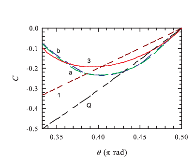
Our results are plotted in Fig. 5; they are consistent with the WHCMH. They also show that θmaxw<π2\theta_{\rm max}^{\text{w}}<\frac{\pi}{2}, because they show that there exists a colouring xx with Cx​(θ)<C1​(θ)C_{x}(\theta)<C_{1}(\theta) for some angles θ∈(0,π2)\theta\in\bigl(0,\frac{\pi}{2}\bigr), namely colouring 3 for angles θ∈[0.405​π,π2)\theta\in\bigl[0.405\pi,\frac{\pi}{2}\bigr).

Refer to caption
Figure 5: Correlations computed with (4), subject to the constraint (6), for the colouring functions axa_{x} shown schematically in Fig. 1 and defined in Appendix C.1. The correlations for colouring 2, 3 and 4 are blue dot-dashed, red solid and green dashed curves, respectively. The black dot-dash-dotted curve represents the singlet-state quantum correlation Q⁡(θ)Q(\theta). The dark red dotted and dark green dash-dotted curves show respectively the colouring 11 correlation, C1​(θ)C_{1}(\theta), and anticorrelation, −C1​(θ)-C_{1}(\theta). The gray solid straight lines show the bounds given by Theorem 1, for θ≥π12\theta\geq\frac{\pi}{12}.

Another interesting result is that there exist colourings that produce correlations Cx​(θ)<Q​(θ)C_{x}(\theta)<Q(\theta) for θ\theta close to π2\frac{\pi}{2}: colouring 3 for angles θ∈[0.467​π,π2)\theta\in\bigl[0.467\pi,\frac{\pi}{2}\bigr). It is interesting to find other colourings whose correlations satisfy Cx​(θ)<C1​(θ)C_{x}(\theta)<C_{1}(\theta) and Cx​(θ)<Q​(θ)C_{x}(\theta)<Q(\theta) for angles θ\theta closer to zero. For this purpose, we consider colouring 3δ3_{\delta}, which is defined in Appendix C.1 and consists of a small variation of colouring 3 in terms of the parameter δ\delta. Colouring 3δ3_{\delta} reduces to colouring 33 if δ=0\delta=0. For values of δ\delta in the range [−π18,π24]\bigl[-\frac{\pi}{18},\frac{\pi}{24}\bigr], we obtained that the smallest angle θ\theta for which C3δ​(θ)<C1​(θ)C_{3_{\delta}}(\theta)<C_{1}(\theta) is achieved for δ=−0.038​π\delta=-0.038\pi, in which case we have that C3−0.038​π​(θ)<C1​(θ)C_{3_{-0.038\pi}}(\theta)<C_{1}(\theta) for θ∈[0.386​π,π2)\theta\in\bigl[0.386\pi,\frac{\pi}{2}\bigr). We also obtained that the smallest angle θ\theta for which C3δ​(θ)<Q​(θ)C_{3_{\delta}}(\theta)<Q(\theta) is achieved for δ=−0.046​π\delta=-0.046\pi, in which case we have that C3−0.046​π​(θ)<Q⁡(θ)C_{3_{-0.046\pi}}(\theta)<Q(\theta) for θ∈[0.431​π,π2)\theta\in[0.431\pi,\frac{\pi}{2}\bigr) (see Fig. 6).

Our numerical results imply the bound θmaxw≤0.386​π\theta_{\text{max}}^{\text{w}}\leq 0.386\pi. They also imply that θmaxs≤0.375​π\theta_{\text{max}}^{\text{s}}\leq 0.375\pi, because C2​(θ)>−C1​(θ)C_{2}(\theta)>-C_{1}(\theta) for θ∈(0.375​π,π2)\theta\in\bigl(0.375\pi,\frac{\pi}{2}\bigr), and C1​(θ)≤Cx​(θ)≤−C1​(θ)C_{1}(\theta)\leq C_{x}(\theta)\leq-C_{1}(\theta) for x=2,3,4,3δx=2,3,4,3_{\delta} and θ∈[0,0.375​π]\theta\in[0,0.375\pi].

The slightly improved bound θmaxs≤0.345​π\theta_{\text{max}}^{\text{s}}\leq 0.345\pi was obtained in [19] from a variation of colouring 22, colouring 2Δ2_{\Delta}, in which the polar angle defining the boundary between the black and white regions in the northern hemisphere (see Fig. 1) is reduced by the angle Δ∈[0,π12]\Delta\in\bigl[0,\frac{\pi}{12}\bigr].

Refer to caption
Figure 6: Correlations obtained for colouring 3δ3_{\delta}, defined in Appendix C.1, for δ=−0.038​π\delta=-0.038\pi (a, green dashed curve) and δ=−0.046​π\delta=-0.046\pi (b, blue dot-dashed curve); for colourings 3, 1 and the singlet-state quantum correlation Q⁡(θ)Q(\theta) (red solid, dark red dotted and black dot-dash-dotted curves, respectively).

In order to confirm analytically the numerical observation that there exist colouring functions x∈𝒳x\in\mathcal{X} such that Cx​(θ)<Q​(θ)C_{x}(\theta)<Q(\theta) for θ\theta close to π2\frac{\pi}{2}, we computed C3​(π2−τ)C_{3}\bigl(\frac{\pi}{2}-\tau\bigr) for 0≤τ≪10\leq\tau\ll 1 to order 𝒪⁡(τ2)\mathcal{O}(\tau^{2}). The computation is presented in Appendix C.3. We obtain

C3​(π2−τ)=−1.5​τ+𝒪⁡(τ2).C_{3}\Bigl(\frac{\pi}{2}-\tau\Bigr)=-1.5\tau+\mathcal{O}(\tau^{2}). (17)

On the other hand, the quantum correlation gives Q⁡(π2−τ)=−cos⁡(π2−τ)=−τ+𝒪⁡(τ3).Q\bigl(\frac{\pi}{2}-\tau\bigr)=-\cos\bigl(\frac{\pi}{2}-\tau\bigr)=-\tau+\mathcal{O}(\tau^{3}). Thus, we see that for τ\tau small enough, indeed C3​(π2−τ)<Q⁡(π2−τ)C_{3}\bigl(\frac{\pi}{2}-\tau\bigr)<Q\bigl(\frac{\pi}{2}-\tau\bigr).

Further numerical investigations of the WHCMH and SHCMH might well shed further light on the questions we explore here. For example, one could define an antipodal colouring function xx as the sign of a sum of spherical harmonics, sgn⁡(∑m=−ll∑l=0Lal​m​Yl​m​(ϵ,ϕ)){\rm sgn}(\sum_{m=-l}^{l}\sum_{l=0}^{L}a_{lm}Y_{lm}(\epsilon,\phi)), where the coefficients al​ma_{lm} are variable parameters, and then search for the minimum value of Cx​(θ)C_{x}(\theta), for any given θ\theta, among such functions by optimizing with respect to the al​ma_{lm}. As an ansatz, one might assume that components corresponding to spherical harmonics that oscillate rapidly compared to θ\theta are relatively negligible, given that the colourings defined by such functions contain black and white areas small compared to θ\theta everywhere on the sphere, giving a contribution to the correlation very close to zero. This would allow searches over a finite set of parameters, for any given θ\theta, while the ansatz itself can be tested by finding how the maximum changes with increasing LL.

C.1 Definitions of the colouring functions

In general, a colouring function axa_{x} with azimuthal symmetry can be defined in terms of the set ℰx\mathcal{E}_{x} in which it takes the value 1 as follows:

ax​(ϵ)≡{1if ​ϵ∈ℰx,−1if ​ϵ∈[0,π]/ℰx,\displaystyle a_{x}(\epsilon)\equiv\left\{\begin{array}[]{rl}1&\text{if }\epsilon\in\mathcal{E}_{x},\\ -1&\text{if }\epsilon\in[0,\pi]/\mathcal{E}_{x},\end{array}\right.

where ϵ∈[0,π]\epsilon\in[0,\pi] is the polar angle in the sphere. For the colourings that we have considered here, x=1,2,3,4,3δx=1,2,3,4,3_{\delta}, we define

ℰ1\displaystyle\mathcal{E}_{1} ≡[0,π2],\displaystyle\equiv\biggl[0,\frac{\pi}{2}\biggr],
ℰ2\displaystyle\mathcal{E}_{2} ≡[0,π4]​⋃[π2,3​π4],\displaystyle\equiv\biggl[0,\frac{\pi}{4}\biggr]\bigcup\biggl[\frac{\pi}{2},\frac{3\pi}{4}\biggr],
ℰ3\displaystyle\mathcal{E}_{3} ≡⋃k=02[k​π3,(2​k+1)​π6],\displaystyle\equiv\bigcup_{k=0}^{2}\biggl[k\frac{\pi}{3},(2k+1)\frac{\pi}{6}\biggr],
ℰ4\displaystyle\mathcal{E}_{4} ≡⋃k=03[k​π4,(2​k+1)​π8],\displaystyle\equiv\bigcup_{k=0}^{3}\biggl[k\frac{\pi}{4},(2k+1)\frac{\pi}{8}\biggr],
ℰ3δ\displaystyle\mathcal{E}_{3_{\delta}} ≡[0,π6+δ]​⋃[π3,π2]​⋃[2​π3,5​π6−δ],\displaystyle\equiv\biggl[0,\frac{\pi}{6}+\delta\biggr]\bigcup\biggl[\frac{\pi}{3},\frac{\pi}{2}\biggr]\bigcup\biggl[\frac{2\pi}{3},\frac{5\pi}{6}-\delta\biggr],

where −π18≤δ≤π24-\frac{\pi}{18}\leq\delta\leq\frac{\pi}{24}. Notice that colouring 3δ3_{\delta} reduces to colouring 3 if δ=0\delta=0.

C.2 Expressions for the correlations

We use the azimuthal symmetry of the colourings x=2,3,4,3δx=2,3,4,3_{\delta} defined in Appendix C.1, the antipodal property (2) and the constraint (6) to reduce the correlation given by (4) to:

Cx(θ)=−1π∫0π2dϵsinϵax(ϵ)∫0πdωax[α(θ,ϵ,ω)],C_{x}(\theta)=-\frac{1}{\pi}\int_{0}^{\frac{\pi}{2}}d\epsilon\sin{\epsilon}a_{x}(\epsilon)\int_{0}^{\pi}d\omega a_{x}[\alpha(\theta,\epsilon,\omega)], (22)

where α⁡(θ,ϵ,ω)\alpha(\theta,\epsilon,\omega) is given by Eq. (15). We computed the integral with respect to ω\omega in the previous expression. We define the function

χ⁡(θ,a,b,α)≡2π​∫abd​ϵ​sin⁡ϵ​arccos⁡(cos⁡θ​cos⁡ϵ−cos⁡αsin⁡θ​sin⁡ϵ),\chi(\theta,a,b,\alpha)\equiv\frac{2}{\pi}\int_{a}^{b}d\epsilon\sin\epsilon\arccos\Bigl(\frac{\cos\theta\cos\epsilon-\cos\alpha}{\sin\theta\sin\epsilon}\Bigr), (23)

where a,b,α∈[0,π]a,b,\alpha\in[0,\pi] and θ∈[0,π2]\theta\in\bigl[0,\frac{\pi}{2}\bigr]. We obtained the following expressions for the correlations Cx​(θ)C_{x}(\theta):

C2​(θ)\displaystyle C_{2}(\theta) ={h21​(θ)if ​θ∈[0,π/4],h22​(θ)if ​θ∈(π/4,π/2],\displaystyle=\left\{\begin{array}[]{rl}h_{2}^{1}(\theta)&\text{if }\theta\in[0,\pi/4],\\ h_{2}^{2}(\theta)&\text{if }\theta\in(\pi/4,\pi/2],\\ \end{array}\right.
C3​(θ)\displaystyle C_{3}(\theta) ={h31​(θ)if ​θ∈[0,π/6],h32​(θ)if ​θ∈(π/6,π/4],h33​(θ)if ​θ∈(π/4,π/3],h34​(θ)if ​θ∈(π/3,π/2],\displaystyle=\left\{\begin{array}[]{rl}h_{3}^{1}(\theta)&\text{if }\theta\in[0,\pi/6],\\ h_{3}^{2}(\theta)&\text{if }\theta\in(\pi/6,\pi/4],\\ h_{3}^{3}(\theta)&\text{if }\theta\in(\pi/4,\pi/3],\\ h_{3}^{4}(\theta)&\text{if }\theta\in(\pi/3,\pi/2],\\ \end{array}\right.
C4​(θ)\displaystyle C_{4}(\theta) ={h41​(θ)if ​θ∈[0,π/8],h42​(θ)if ​θ∈(π/8,π/4],h43​(θ)if ​θ∈(π/4,3​π/8],h44​(θ)if ​θ∈(3​π/8,π/2],\displaystyle=\left\{\begin{array}[]{rl}h_{4}^{1}(\theta)&\text{if }\theta\in[0,\pi/8],\\ h_{4}^{2}(\theta)&\text{if }\theta\in(\pi/8,\pi/4],\\ h_{4}^{3}(\theta)&\text{if }\theta\in(\pi/4,3\pi/8],\\ h_{4}^{4}(\theta)&\text{if }\theta\in(3\pi/8,\pi/2],\\ \end{array}\right.
C3δ​(θ)\displaystyle C_{3_{\delta}}(\theta) ={rδ1​(θ)if δ∈[−π18,0] and θ∈[π3,π3−δ],rδ2​(θ)if δ∈[−π18,0] and θ∈(π3−δ,π2+δ],rδ3​(θ)if δ∈[−π18,0] and θ∈(π2+δ,π2],rδ4​(θ)if δ∈(0,π24] and θ∈[π3,π3+2δ],rδ2​(θ)if δ∈(0,π24] and θ∈(π3+2δ,π2−δ],rδ5​(θ)if δ∈(0,π24] and θ∈(π2−δ,π2],\displaystyle=\left\{\begin{array}[]{rl}r_{\delta}^{1}(\theta)&\text{if }\delta\in\bigl[-\frac{\pi}{18},0\bigr]\text{ and }\theta\in\bigl[\frac{\pi}{3},\frac{\pi}{3}-\delta\bigr],\\ r_{\delta}^{2}(\theta)&\text{if }\delta\in\bigl[-\frac{\pi}{18},0\bigr]\text{ and }\theta\in\bigl(\frac{\pi}{3}-\delta,\frac{\pi}{2}+\delta\bigr],\\ r_{\delta}^{3}(\theta)&\text{if }\delta\in\bigl[-\frac{\pi}{18},0\bigr]\text{ and }\theta\in\bigl(\frac{\pi}{2}+\delta,\frac{\pi}{2}\bigr],\\ r_{\delta}^{4}(\theta)&\text{if }\delta\in\bigl(0,\frac{\pi}{24}\bigr]\text{ and }\theta\in\bigl[\frac{\pi}{3},\frac{\pi}{3}+2\delta\bigr],\\ r_{\delta}^{2}(\theta)&\text{if }\delta\in\bigl(0,\frac{\pi}{24}\bigr]\text{ and }\theta\in\bigl(\frac{\pi}{3}+2\delta,\frac{\pi}{2}-\delta\bigr],\\ r_{\delta}^{5}(\theta)&\text{if }\delta\in\bigl(0,\frac{\pi}{24}\bigr]\text{ and }\theta\in\bigl(\frac{\pi}{2}-\delta,\frac{\pi}{2}\bigr],\\ \end{array}\right.

where

h21​(θ)\displaystyle h_{2}^{1}(\theta) ≡−1+2​[cos⁡(π4)−cos⁡(π4+θ)]+χ⁡(θ,π4−θ,π4,π4)−χ⁡(θ,π4,π4+θ,π4)+χ⁡(θ,π2−θ,π2,π2),\displaystyle\equiv-1+2\biggl[\cos\Bigl(\frac{\pi}{4}\Bigr)-\cos\Bigl(\frac{\pi}{4}+\theta\Bigr)\biggr]+\chi\Bigl(\theta,\frac{\pi}{4}-\theta,\frac{\pi}{4},\frac{\pi}{4}\Bigr)-\chi\Bigl(\theta,\frac{\pi}{4},\frac{\pi}{4}+\theta,\frac{\pi}{4}\Bigr)+\chi\Bigl(\theta,\frac{\pi}{2}-\theta,\frac{\pi}{2},\frac{\pi}{2}\Bigr),
h22​(θ)\displaystyle h_{2}^{2}(\theta) ≡1+2​[cos⁡(π4)−cos⁡(θ−π4)]+χ⁡(θ,θ−π4,π4,π4)−χ⁡(θ,π2−θ,π4,π2)+χ⁡(θ,π4,π2,π2)\displaystyle\equiv 1+2\biggl[\cos\Bigl(\frac{\pi}{4}\Bigr)-\cos\Bigl(\theta-\frac{\pi}{4}\Bigr)\biggr]+\chi\Bigl(\theta,\theta-\frac{\pi}{4},\frac{\pi}{4},\frac{\pi}{4}\Bigr)-\chi\Bigl(\theta,\frac{\pi}{2}-\theta,\frac{\pi}{4},\frac{\pi}{2}\Bigr)+\chi\Bigl(\theta,\frac{\pi}{4},\frac{\pi}{2},\frac{\pi}{2}\Bigr)
−χ⁡(θ,π4,π2,π4)−χ⁡(θ,3​π4−θ,π2,3​π4);\displaystyle\qquad-\chi\Bigl(\theta,\frac{\pi}{4},\frac{\pi}{2},\frac{\pi}{4}\Bigr)-\chi\Bigl(\theta,\frac{3\pi}{4}-\theta,\frac{\pi}{2},\frac{3\pi}{4}\Bigr);
h31​(θ)\displaystyle h_{3}^{1}(\theta) ≡−1+2​[cos⁡(π6)−cos⁡(π6+θ)+cos⁡(π3)−cos⁡(π3+θ)]+χ⁡(θ,π6−θ,π6,π6)−χ⁡(θ,π6,π6+θ,π6)\displaystyle\equiv-1+2\biggl[\cos\Bigl(\frac{\pi}{6}\Bigr)-\cos\Bigl(\frac{\pi}{6}+\theta\Bigr)+\cos\Bigl(\frac{\pi}{3}\Bigr)-\cos\Bigl(\frac{\pi}{3}+\theta\Bigr)\Bigr]+\chi\Bigl(\theta,\frac{\pi}{6}-\theta,\frac{\pi}{6},\frac{\pi}{6}\Bigr)-\chi\Bigl(\theta,\frac{\pi}{6},\frac{\pi}{6}+\theta,\frac{\pi}{6}\Bigr)
+χ⁡(θ,π3−θ,π3,π3)−χ⁡(θ,π3,π3+θ,π3)+χ⁡(θ,π2−θ,π2,π2),\displaystyle\qquad+\chi\Bigl(\theta,\frac{\pi}{3}-\theta,\frac{\pi}{3},\frac{\pi}{3}\Bigr)-\chi\Bigl(\theta,\frac{\pi}{3},\frac{\pi}{3}+\theta,\frac{\pi}{3}\Bigr)+\chi\Bigl(\theta,\frac{\pi}{2}-\theta,\frac{\pi}{2},\frac{\pi}{2}\Bigr),
h32​(θ)\displaystyle h_{3}^{2}(\theta) ≡1+2​[cos⁡(π6)−cos⁡(θ−π6)+cos⁡(π6+θ)−cos⁡(π3)]+χ⁡(θ,θ−π6,π6,π6)−χ⁡(θ,π3−θ,π6,π3)\displaystyle\equiv 1+2\biggl[\cos\Bigl(\frac{\pi}{6}\Bigr)-\cos\Bigl(\theta-\frac{\pi}{6}\Bigr)+\cos\Bigl(\frac{\pi}{6}+\theta\Bigr)-\cos\Bigl(\frac{\pi}{3}\Bigr)\Bigr]+\chi\Bigl(\theta,\theta-\frac{\pi}{6},\frac{\pi}{6},\frac{\pi}{6}\Bigr)-\chi\Bigl(\theta,\frac{\pi}{3}-\theta,\frac{\pi}{6},\frac{\pi}{3}\Bigr)
+χ⁡(θ,π6,π2−θ,π3)−χ⁡(θ,π6,π3,π6)+χ⁡(θ,π2−θ,π3,π3)−χ⁡(θ,π2−θ,π3,π2)+χ⁡(θ,π3,π6+θ,π6)\displaystyle\qquad+\chi\Bigl(\theta,\frac{\pi}{6},\frac{\pi}{2}-\theta,\frac{\pi}{3}\Bigr)-\chi\Bigl(\theta,\frac{\pi}{6},\frac{\pi}{3},\frac{\pi}{6}\Bigr)+\chi\Bigl(\theta,\frac{\pi}{2}-\theta,\frac{\pi}{3},\frac{\pi}{3}\Bigr)-\chi\Bigl(\theta,\frac{\pi}{2}-\theta,\frac{\pi}{3},\frac{\pi}{2}\Bigr)+\chi\Bigl(\theta,\frac{\pi}{3},\frac{\pi}{6}+\theta,\frac{\pi}{6}\Bigr)
+χ⁡(θ,π3,π2,π2)−χ⁡(θ,π3,π2,π3)−χ⁡(θ,2​π3−θ,π2,2​π3),\displaystyle\qquad+\chi\Bigl(\theta,\frac{\pi}{3},\frac{\pi}{2},\frac{\pi}{2}\Bigr)-\chi\Bigl(\theta,\frac{\pi}{3},\frac{\pi}{2},\frac{\pi}{3}\Bigr)-\chi\Bigl(\theta,\frac{2\pi}{3}-\theta,\frac{\pi}{2},\frac{2\pi}{3}\Bigr),
h33​(θ)\displaystyle h_{3}^{3}(\theta) ≡1+2​[cos⁡(π6)−cos⁡(θ−π6)+cos⁡(π6+θ)−cos⁡(π3)]−χ⁡(θ,π3−θ,π6,π3)+χ⁡(θ,θ−π6,π6,π6)\displaystyle\equiv 1+2\biggl[\cos\Bigl(\frac{\pi}{6}\Bigr)-\cos\Bigl(\theta-\frac{\pi}{6}\Bigr)+\cos\Bigl(\frac{\pi}{6}+\theta\Bigr)-\cos\Bigl(\frac{\pi}{3}\Bigr)\Bigr]-\chi\Bigl(\theta,\frac{\pi}{3}-\theta,\frac{\pi}{6},\frac{\pi}{3}\Bigr)+\chi\Bigl(\theta,\theta-\frac{\pi}{6},\frac{\pi}{6},\frac{\pi}{6}\Bigr)
+χ⁡(θ,π6,π3,π3)−χ⁡(θ,π6,π3,π6)−χ⁡(θ,π2−θ,π3,π2)+χ⁡(θ,π3,π2,π2)−χ⁡(θ,π3,π2,π3)\displaystyle\qquad+\chi\Bigl(\theta,\frac{\pi}{6},\frac{\pi}{3},\frac{\pi}{3}\Bigr)-\chi\Bigl(\theta,\frac{\pi}{6},\frac{\pi}{3},\frac{\pi}{6}\Bigr)-\chi\Bigl(\theta,\frac{\pi}{2}-\theta,\frac{\pi}{3},\frac{\pi}{2}\Bigr)+\chi\Bigl(\theta,\frac{\pi}{3},\frac{\pi}{2},\frac{\pi}{2}\Bigr)-\chi\Bigl(\theta,\frac{\pi}{3},\frac{\pi}{2},\frac{\pi}{3}\Bigr)
+χ⁡(θ,π3,π6+θ,π6)−χ⁡(θ,2​π3−θ,π2,2​π3),\displaystyle\qquad+\chi\Bigl(\theta,\frac{\pi}{3},\frac{\pi}{6}+\theta,\frac{\pi}{6}\Bigr)-\chi\Bigl(\theta,\frac{2\pi}{3}-\theta,\frac{\pi}{2},\frac{2\pi}{3}\Bigr),
h34​(θ)\displaystyle h_{3}^{4}(\theta) ≡−1+2​[cos⁡(θ−π3)−cos⁡(π6)+cos⁡(θ−π6)−cos⁡(π3)]−χ⁡(θ,θ−π3,π6,π3)+χ⁡(θ,π2−θ,π6,π2)\displaystyle\equiv-1+2\biggl[\cos\Bigl(\theta-\frac{\pi}{3}\Bigr)-\cos\Bigl(\frac{\pi}{6}\Bigr)+\cos\Bigl(\theta-\frac{\pi}{6}\Bigr)-\cos\Bigl(\frac{\pi}{3}\Bigr)\Bigr]-\chi\Bigl(\theta,\theta-\frac{\pi}{3},\frac{\pi}{6},\frac{\pi}{3}\Bigr)+\chi\Bigl(\theta,\frac{\pi}{2}-\theta,\frac{\pi}{6},\frac{\pi}{2}\Bigr)
+χ⁡(θ,π6,π3,π3)−χ⁡(θ,π6,π3,π2)−χ⁡(θ,θ−π6,π3,π6)+χ⁡(θ,2​π3−θ,π3,2​π3)−χ⁡(θ,π3,π2,2​π3)\displaystyle\qquad+\chi\Bigl(\theta,\frac{\pi}{6},\frac{\pi}{3},\frac{\pi}{3}\Bigr)-\chi\Bigl(\theta,\frac{\pi}{6},\frac{\pi}{3},\frac{\pi}{2}\Bigr)-\chi\Bigl(\theta,\theta-\frac{\pi}{6},\frac{\pi}{3},\frac{\pi}{6}\Bigr)+\chi\Bigl(\theta,\frac{2\pi}{3}-\theta,\frac{\pi}{3},\frac{2\pi}{3}\Bigr)-\chi\Bigl(\theta,\frac{\pi}{3},\frac{\pi}{2},\frac{2\pi}{3}\Bigr)
+χ⁡(θ,π3,π2,π2)−χ⁡(θ,π3,π2,π3)+χ⁡(θ,π3,π2,π6)+χ⁡(θ,5​π6−θ,π2,5​π6);\displaystyle\qquad+\chi\Bigl(\theta,\frac{\pi}{3},\frac{\pi}{2},\frac{\pi}{2}\Bigr)-\chi\Bigl(\theta,\frac{\pi}{3},\frac{\pi}{2},\frac{\pi}{3}\Bigr)+\chi\Bigl(\theta,\frac{\pi}{3},\frac{\pi}{2},\frac{\pi}{6}\Bigr)+\chi\Bigl(\theta,\frac{5\pi}{6}-\theta,\frac{\pi}{2},\frac{5\pi}{6}\Bigr);
h41​(θ)\displaystyle h_{4}^{1}(\theta) ≡−1+2​[cos⁡(π8)−cos⁡(π8+θ)+cos⁡(π4)−cos⁡(π4+θ)+cos⁡(3​π8)−cos⁡(3​π8+θ)]+χ⁡(θ,π8−θ,π8,π8)\displaystyle\equiv-1+2\biggl[\cos\Bigl(\frac{\pi}{8}\Bigr)-\cos\Bigl(\frac{\pi}{8}+\theta\Bigr)+\cos\Bigl(\frac{\pi}{4}\Bigr)-\cos\Bigl(\frac{\pi}{4}+\theta\Bigr)+\cos\Bigl(\frac{3\pi}{8}\Bigr)-\cos\Bigl(\frac{3\pi}{8}+\theta\Bigr)\biggr]+\chi\Bigl(\theta,\frac{\pi}{8}-\theta,\frac{\pi}{8},\frac{\pi}{8}\Bigr)
−χ⁡(θ,π8,π8+θ,π8)+χ⁡(θ,π4−θ,π4,π4)−χ⁡(θ,π4,π4+θ,π4)+χ⁡(θ,3​π8−θ,3​π8,3​π8)\displaystyle\qquad-\chi\Bigl(\theta,\frac{\pi}{8},\frac{\pi}{8}+\theta,\frac{\pi}{8}\Bigr)+\chi\Bigl(\theta,\frac{\pi}{4}-\theta,\frac{\pi}{4},\frac{\pi}{4}\Bigr)-\chi\Bigl(\theta,\frac{\pi}{4},\frac{\pi}{4}+\theta,\frac{\pi}{4}\Bigr)+\chi\Bigl(\theta,\frac{3\pi}{8}-\theta,\frac{3\pi}{8},\frac{3\pi}{8}\Bigr)
−χ⁡(θ,3​π8,3​π8+θ,3​π8)+χ⁡(θ,π2−θ,π2,π2),\displaystyle\qquad-\chi\Bigl(\theta,\frac{3\pi}{8},\frac{3\pi}{8}+\theta,\frac{3\pi}{8}\Bigr)+\chi\Bigl(\theta,\frac{\pi}{2}-\theta,\frac{\pi}{2},\frac{\pi}{2}\Bigr),
h42​(θ)\displaystyle h_{4}^{2}(\theta) ≡1+2​[cos⁡(π8)−cos⁡(θ−π8)+cos⁡(θ+π8)−cos⁡(π4)+cos⁡(θ+π4)−cos⁡(3​π8)]+χ⁡(θ,θ−π8,π8,π8)\displaystyle\equiv 1+2\biggl[\cos\Bigl(\frac{\pi}{8}\Bigr)-\cos\Bigl(\theta-\frac{\pi}{8}\Bigr)+\cos\Bigl(\theta+\frac{\pi}{8}\Bigr)-\cos\Bigl(\frac{\pi}{4}\Bigr)+\cos\Bigl(\theta+\frac{\pi}{4}\Bigr)-\cos\Bigl(\frac{3\pi}{8}\Bigr)\biggr]+\chi\Bigl(\theta,\theta-\frac{\pi}{8},\frac{\pi}{8},\frac{\pi}{8}\Bigr)
−χ⁡(θ,π4−θ,π8,π4)+χ⁡(θ,π8,π4,π4)−χ⁡(θ,π8,π4,π8)−χ⁡(θ,3​π8−θ,π4,3​π8)+χ⁡(θ,π4,π8+θ,π8)\displaystyle\qquad-\chi\Bigl(\theta,\frac{\pi}{4}-\theta,\frac{\pi}{8},\frac{\pi}{4}\Bigr)+\chi\Bigl(\theta,\frac{\pi}{8},\frac{\pi}{4},\frac{\pi}{4}\Bigr)-\chi\Bigl(\theta,\frac{\pi}{8},\frac{\pi}{4},\frac{\pi}{8}\Bigr)-\chi\Bigl(\theta,\frac{3\pi}{8}-\theta,\frac{\pi}{4},\frac{3\pi}{8}\Bigr)+\chi\Bigl(\theta,\frac{\pi}{4},\frac{\pi}{8}+\theta,\frac{\pi}{8}\Bigr)
+χ⁡(θ,π4,3​π8,3​π8)−χ⁡(θ,π4,3​π8,π4)−χ⁡(θ,π2−θ,3​π8,π2)+χ⁡(θ,3​π8,π4+θ,π4)+χ⁡(θ,3​π8,π2,π2)\displaystyle\qquad+\chi\Bigl(\theta,\frac{\pi}{4},\frac{3\pi}{8},\frac{3\pi}{8}\Bigr)-\chi\Bigl(\theta,\frac{\pi}{4},\frac{3\pi}{8},\frac{\pi}{4}\Bigr)-\chi\Bigl(\theta,\frac{\pi}{2}-\theta,\frac{3\pi}{8},\frac{\pi}{2}\Bigr)+\chi\Bigl(\theta,\frac{3\pi}{8},\frac{\pi}{4}+\theta,\frac{\pi}{4}\Bigr)+\chi\Bigl(\theta,\frac{3\pi}{8},\frac{\pi}{2},\frac{\pi}{2}\Bigr)
−χ⁡(θ,3​π8,π2,3​π8)−χ⁡(θ,5​π8−θ,π2,5​π8),\displaystyle\qquad-\chi\Bigl(\theta,\frac{3\pi}{8},\frac{\pi}{2},\frac{3\pi}{8}\Bigr)-\chi\Bigl(\theta,\frac{5\pi}{8}-\theta,\frac{\pi}{2},\frac{5\pi}{8}\Bigr),
h43​(θ)\displaystyle h_{4}^{3}(\theta) ≡−1+2​[cos⁡(θ−π4)−cos⁡(π8)+cos⁡(θ−π8)−cos⁡(π4)+cos⁡(3​π8)−cos⁡(θ+π8)]−χ⁡(θ,θ−π4,π8,π4)\displaystyle\equiv-1+2\biggl[\cos\Bigl(\theta-\frac{\pi}{4}\Bigr)-\cos\Bigl(\frac{\pi}{8}\Bigr)+\cos\Bigl(\theta-\frac{\pi}{8}\Bigr)-\cos\Bigl(\frac{\pi}{4}\Bigr)+\cos\Bigl(\frac{3\pi}{8}\Bigr)-\cos\Bigl(\theta+\frac{\pi}{8}\Bigr)\biggr]-\chi\Bigl(\theta,\theta-\frac{\pi}{4},\frac{\pi}{8},\frac{\pi}{4}\Bigr)
+χ⁡(θ,3​π8−θ,π8,3​π8)−χ⁡(θ,π8,π4,3​π8)+χ⁡(θ,π8,π4,π4)−χ⁡(θ,θ−π8,π4,π8)+χ⁡(θ,π2−θ,π4,π2)\displaystyle\qquad+\chi\Bigl(\theta,\frac{3\pi}{8}-\theta,\frac{\pi}{8},\frac{3\pi}{8}\Bigr)-\chi\Bigl(\theta,\frac{\pi}{8},\frac{\pi}{4},\frac{3\pi}{8}\Bigr)+\chi\Bigl(\theta,\frac{\pi}{8},\frac{\pi}{4},\frac{\pi}{4}\Bigr)-\chi\Bigl(\theta,\theta-\frac{\pi}{8},\frac{\pi}{4},\frac{\pi}{8}\Bigr)+\chi\Bigl(\theta,\frac{\pi}{2}-\theta,\frac{\pi}{4},\frac{\pi}{2}\Bigr)
−χ⁡(θ,π4,3​π8,π2)+χ⁡(θ,π4,3​π8,3​π8)−χ⁡(θ,π4,3​π8,π4)+χ⁡(θ,π4,3​π8,π8)+χ⁡(θ,5​π8−θ,3​π8,5​π8)\displaystyle\qquad-\chi\Bigl(\theta,\frac{\pi}{4},\frac{3\pi}{8},\frac{\pi}{2}\Bigr)+\chi\Bigl(\theta,\frac{\pi}{4},\frac{3\pi}{8},\frac{3\pi}{8}\Bigr)-\chi\Bigl(\theta,\frac{\pi}{4},\frac{3\pi}{8},\frac{\pi}{4}\Bigr)+\chi\Bigl(\theta,\frac{\pi}{4},\frac{3\pi}{8},\frac{\pi}{8}\Bigr)+\chi\Bigl(\theta,\frac{5\pi}{8}-\theta,\frac{3\pi}{8},\frac{5\pi}{8}\Bigr)
−χ⁡(θ,3​π8,π2,5​π8)+χ⁡(θ,3​π8,π2,π2)−χ⁡(θ,3​π8,π2,3​π8)+χ⁡(θ,3​π8,π2,π4)−χ⁡(θ,3​π8,π8+θ,π8)\displaystyle\qquad-\chi\Bigl(\theta,\frac{3\pi}{8},\frac{\pi}{2},\frac{5\pi}{8}\Bigr)+\chi\Bigl(\theta,\frac{3\pi}{8},\frac{\pi}{2},\frac{\pi}{2}\Bigr)-\chi\Bigl(\theta,\frac{3\pi}{8},\frac{\pi}{2},\frac{3\pi}{8}\Bigr)+\chi\Bigl(\theta,\frac{3\pi}{8},\frac{\pi}{2},\frac{\pi}{4}\Bigr)-\chi\Bigl(\theta,\frac{3\pi}{8},\frac{\pi}{8}+\theta,\frac{\pi}{8}\Bigr)
+χ⁡(θ,3​π4−θ,π2,3​π4),\displaystyle\qquad+\chi\Bigl(\theta,\frac{3\pi}{4}-\theta,\frac{\pi}{2},\frac{3\pi}{4}\Bigr),
h44​(θ)\displaystyle h_{4}^{4}(\theta) ≡1+2​[cos⁡(π8)−cos⁡(θ−3​π8)+cos⁡(π4)−cos⁡(θ−π4)+cos⁡(3​π8)−cos⁡(θ−π8)]+χ⁡(θ,θ−3​π8,π8,3​π8)\displaystyle\equiv 1+2\biggl[\cos\Bigl(\frac{\pi}{8}\Bigr)-\cos\Bigl(\theta-\frac{3\pi}{8}\Bigr)+\cos\Bigl(\frac{\pi}{4}\Bigr)-\cos\Bigl(\theta-\frac{\pi}{4}\Bigr)+\cos\Bigl(\frac{3\pi}{8}\Bigr)-\cos\Bigl(\theta-\frac{\pi}{8}\Bigr)\biggr]+\chi\Bigl(\theta,\theta-\frac{3\pi}{8},\frac{\pi}{8},\frac{3\pi}{8}\Bigr)
−χ⁡(θ,π2−θ,π8,π2)+χ⁡(θ,π8,π4,π2)−χ⁡(θ,π8,π4,3​π8)+χ⁡(θ,θ−π4,π4,π4)−χ⁡(θ,5​π8−θ,π4,5​π8)\displaystyle\qquad-\chi\Bigl(\theta,\frac{\pi}{2}-\theta,\frac{\pi}{8},\frac{\pi}{2}\Bigr)+\chi\Bigl(\theta,\frac{\pi}{8},\frac{\pi}{4},\frac{\pi}{2}\Bigr)-\chi\Bigl(\theta,\frac{\pi}{8},\frac{\pi}{4},\frac{3\pi}{8}\Bigr)+\chi\Bigl(\theta,\theta-\frac{\pi}{4},\frac{\pi}{4},\frac{\pi}{4}\Bigr)-\chi\Bigl(\theta,\frac{5\pi}{8}-\theta,\frac{\pi}{4},\frac{5\pi}{8}\Bigr)
+χ⁡(θ,π4,3​π8,5​π8)−χ⁡(θ,π4,3​π8,π2)+χ⁡(θ,π4,3​π8,3​π8)−χ⁡(θ,π4,3​π8,π4)+χ⁡(θ,θ−π8,3​π8,π8)\displaystyle\qquad+\chi\Bigl(\theta,\frac{\pi}{4},\frac{3\pi}{8},\frac{5\pi}{8}\Bigr)-\chi\Bigl(\theta,\frac{\pi}{4},\frac{3\pi}{8},\frac{\pi}{2}\Bigr)+\chi\Bigl(\theta,\frac{\pi}{4},\frac{3\pi}{8},\frac{3\pi}{8}\Bigr)-\chi\Bigl(\theta,\frac{\pi}{4},\frac{3\pi}{8},\frac{\pi}{4}\Bigr)+\chi\Bigl(\theta,\theta-\frac{\pi}{8},\frac{3\pi}{8},\frac{\pi}{8}\Bigr)
−χ⁡(θ,3​π4−θ,3​π8,3​π4)+χ⁡(θ,3​π8,π2,3​π4)−χ⁡(θ,3​π8,π2,5​π8)+χ⁡(θ,3​π8,π2,π2)−χ⁡(θ,3​π8,π2,3​π8)\displaystyle\qquad-\chi\Bigl(\theta,\frac{3\pi}{4}-\theta,\frac{3\pi}{8},\frac{3\pi}{4}\Bigr)+\chi\Bigl(\theta,\frac{3\pi}{8},\frac{\pi}{2},\frac{3\pi}{4}\Bigr)-\chi\Bigl(\theta,\frac{3\pi}{8},\frac{\pi}{2},\frac{5\pi}{8}\Bigr)+\chi\Bigl(\theta,\frac{3\pi}{8},\frac{\pi}{2},\frac{\pi}{2}\Bigr)-\chi\Bigl(\theta,\frac{3\pi}{8},\frac{\pi}{2},\frac{3\pi}{8}\Bigr)
+χ⁡(θ,3​π8,π2,π4)−χ⁡(θ,3​π8,π2,π8)−χ⁡(θ,7​π8−θ,π2,7​π8);\displaystyle\qquad+\chi\Bigl(\theta,\frac{3\pi}{8},\frac{\pi}{2},\frac{\pi}{4}\Bigr)-\chi\Bigl(\theta,\frac{3\pi}{8},\frac{\pi}{2},\frac{\pi}{8}\Bigr)-\chi\Bigl(\theta,\frac{7\pi}{8}-\theta,\frac{\pi}{2},\frac{7\pi}{8}\Bigr);
rδ1​(θ)\displaystyle r_{\delta}^{1}(\theta) ≡−1+2​[cos⁡(θ−π3)−cos⁡(π6+δ)+cos⁡(θ−π6−δ)−cos⁡(π3)+cos⁡(θ+π6+δ)]\displaystyle\equiv-1+2\biggl[\cos\Bigl(\theta-\frac{\pi}{3}\Bigr)-\cos\Bigl(\frac{\pi}{6}+\delta\Bigr)+\cos\Bigl(\theta-\frac{\pi}{6}-\delta\Bigr)-\cos\Bigl(\frac{\pi}{3}\Bigr)+\cos\Bigl(\theta+\frac{\pi}{6}+\delta\Bigr)\biggr]
−χ⁡(θ,θ−π3,π6+δ,π3)+χ⁡(θ,π6+δ,π3,π3)−χ⁡(θ,π2−θ,π3,π2)−χ⁡(θ,θ−π6−δ,π3,π6+δ)\displaystyle\qquad-\chi\Bigl(\theta,\theta-\frac{\pi}{3},\frac{\pi}{6}+\delta,\frac{\pi}{3}\Bigr)+\chi\Bigl(\theta,\frac{\pi}{6}+\delta,\frac{\pi}{3},\frac{\pi}{3}\Bigr)-\chi\Bigl(\theta,\frac{\pi}{2}-\theta,\frac{\pi}{3},\frac{\pi}{2}\Bigr)-\chi\Bigl(\theta,\theta-\frac{\pi}{6}-\delta,\frac{\pi}{3},\frac{\pi}{6}+\delta\Bigr)
+χ⁡(θ,2​π3−θ,π3,2​π3)−χ⁡(θ,π3,π2,2​π3)+χ⁡(θ,π3,π2,π2)−χ⁡(θ,π3,π2,π3)+χ⁡(θ,π3,θ+π6+δ,π6+δ),\displaystyle\qquad+\chi\Bigl(\theta,\frac{2\pi}{3}-\theta,\frac{\pi}{3},\frac{2\pi}{3}\Bigr)-\chi\Bigl(\theta,\frac{\pi}{3},\frac{\pi}{2},\frac{2\pi}{3}\Bigr)+\chi\Bigl(\theta,\frac{\pi}{3},\frac{\pi}{2},\frac{\pi}{2}\Bigr)-\chi\Bigl(\theta,\frac{\pi}{3},\frac{\pi}{2},\frac{\pi}{3}\Bigr)+\chi\Bigl(\theta,\frac{\pi}{3},\theta+\frac{\pi}{6}+\delta,\frac{\pi}{6}+\delta\Bigr),
rδ2​(θ)\displaystyle r_{\delta}^{2}(\theta) ≡−1+2​[cos⁡(θ−π3)−cos⁡(π6+δ)+cos⁡(θ−π6−δ)−cos⁡(π3)]−χ⁡(θ,θ−π3,π6+δ,π3)\displaystyle\equiv-1+2\biggl[\cos\Bigl(\theta-\frac{\pi}{3}\Bigr)-\cos\Bigl(\frac{\pi}{6}+\delta\Bigr)+\cos\Bigl(\theta-\frac{\pi}{6}-\delta\Bigr)-\cos\Bigl(\frac{\pi}{3}\Bigr)\biggr]-\chi\Bigl(\theta,\theta-\frac{\pi}{3},\frac{\pi}{6}+\delta,\frac{\pi}{3}\Bigr)
+χ⁡(θ,π2−θ,π6+δ,π2)−χ⁡(θ,π6+δ,π3,π2)+χ⁡(θ,π6+δ,π3,π3)−χ⁡(θ,θ−π6−δ,π3,π6+δ)\displaystyle\qquad+\chi\Bigl(\theta,\frac{\pi}{2}-\theta,\frac{\pi}{6}+\delta,\frac{\pi}{2}\Bigr)-\chi\Bigl(\theta,\frac{\pi}{6}+\delta,\frac{\pi}{3},\frac{\pi}{2}\Bigr)+\chi\Bigl(\theta,\frac{\pi}{6}+\delta,\frac{\pi}{3},\frac{\pi}{3}\Bigr)-\chi\Bigl(\theta,\theta-\frac{\pi}{6}-\delta,\frac{\pi}{3},\frac{\pi}{6}+\delta\Bigr)
+χ⁡(θ,2​π3−θ,π3,2​π3)−χ⁡(θ,π3,π2,2​π3)+χ⁡(θ,π3,π2,π2)−χ⁡(θ,π3,π2,π3)+χ⁡(θ,π3,π2,π6+δ)\displaystyle\qquad+\chi\Bigl(\theta,\frac{2\pi}{3}-\theta,\frac{\pi}{3},\frac{2\pi}{3}\Bigr)-\chi\Bigl(\theta,\frac{\pi}{3},\frac{\pi}{2},\frac{2\pi}{3}\Bigr)+\chi\Bigl(\theta,\frac{\pi}{3},\frac{\pi}{2},\frac{\pi}{2}\Bigr)-\chi\Bigl(\theta,\frac{\pi}{3},\frac{\pi}{2},\frac{\pi}{3}\Bigr)+\chi\Bigl(\theta,\frac{\pi}{3},\frac{\pi}{2},\frac{\pi}{6}+\delta\Bigr)
+χ⁡(θ,5​π6−δ−θ,π2,5​π6−δ),\displaystyle\qquad+\chi\Bigl(\theta,\frac{5\pi}{6}-\delta-\theta,\frac{\pi}{2},\frac{5\pi}{6}-\delta\Bigr),
rδ3​(θ)\displaystyle r_{\delta}^{3}(\theta) ≡−1+2​[cos⁡(π6+δ)−cos⁡(θ−π3)+cos⁡(π3)−cos⁡(θ−π6−δ)]+χ⁡(θ,π2−θ,π6+δ,π2)\displaystyle\equiv-1+2\biggl[\cos\Bigl(\frac{\pi}{6}+\delta\Bigr)-\cos\Bigl(\theta-\frac{\pi}{3}\Bigr)+\cos\Bigl(\frac{\pi}{3}\Bigr)-\cos\Bigl(\theta-\frac{\pi}{6}-\delta\Bigr)\biggr]+\chi\Bigl(\theta,\frac{\pi}{2}-\theta,\frac{\pi}{6}+\delta,\frac{\pi}{2}\Bigr)
−χ⁡(θ,π6+δ,π3,π2)+χ⁡(θ,θ−π3,π3,π3)+χ⁡(θ,2​π3−θ,π3,2​π3)−χ⁡(θ,π3,π2,2​π3)+χ⁡(θ,π3,π2,π2)\displaystyle\qquad-\chi\Bigl(\theta,\frac{\pi}{6}+\delta,\frac{\pi}{3},\frac{\pi}{2}\Bigr)+\chi\Bigl(\theta,\theta-\frac{\pi}{3},\frac{\pi}{3},\frac{\pi}{3}\Bigr)+\chi\Bigl(\theta,\frac{2\pi}{3}-\theta,\frac{\pi}{3},\frac{2\pi}{3}\Bigr)-\chi\Bigl(\theta,\frac{\pi}{3},\frac{\pi}{2},\frac{2\pi}{3}\Bigr)+\chi\Bigl(\theta,\frac{\pi}{3},\frac{\pi}{2},\frac{\pi}{2}\Bigr)
−χ⁡(θ,π3,π2,π3)+χ⁡(θ,θ−π6−δ,π2,π6+δ)+χ⁡(θ,5​π6−δ−θ,π2,5​π6−δ),\displaystyle\qquad-\chi\Bigl(\theta,\frac{\pi}{3},\frac{\pi}{2},\frac{\pi}{3}\Bigr)+\chi\Bigl(\theta,\theta-\frac{\pi}{6}-\delta,\frac{\pi}{2},\frac{\pi}{6}+\delta\Bigr)+\chi\Bigl(\theta,\frac{5\pi}{6}-\delta-\theta,\frac{\pi}{2},\frac{5\pi}{6}-\delta\Bigr),
rδ4​(θ)\displaystyle r_{\delta}^{4}(\theta) ≡−1+2​[cos⁡(θ−π3)−cos⁡(θ−π6−δ)+cos⁡(π6+δ)−cos⁡(π3)]−χ⁡(θ,θ−π3,π6+δ,π3)\displaystyle\equiv-1+2\biggl[\cos\Bigl(\theta-\frac{\pi}{3}\Bigr)-\cos\Bigl(\theta-\frac{\pi}{6}-\delta\Bigr)+\cos\Bigl(\frac{\pi}{6}+\delta\Bigr)-\cos\Bigl(\frac{\pi}{3}\Bigr)\biggr]-\chi\Bigl(\theta,\theta-\frac{\pi}{3},\frac{\pi}{6}+\delta,\frac{\pi}{3}\Bigr)
+χ⁡(θ,θ−π6−δ,π6+δ,π6+δ)+χ⁡(θ,π2−θ,π6+δ,π2)−χ⁡(θ,π6+δ,π3,π2)+χ⁡(θ,π6+δ,π3,π3)\displaystyle\qquad+\chi\Bigl(\theta,\theta-\frac{\pi}{6}-\delta,\frac{\pi}{6}+\delta,\frac{\pi}{6}+\delta\Bigr)+\chi\Bigl(\theta,\frac{\pi}{2}-\theta,\frac{\pi}{6}+\delta,\frac{\pi}{2}\Bigr)-\chi\Bigl(\theta,\frac{\pi}{6}+\delta,\frac{\pi}{3},\frac{\pi}{2}\Bigr)+\chi\Bigl(\theta,\frac{\pi}{6}+\delta,\frac{\pi}{3},\frac{\pi}{3}\Bigr)
−χ⁡(θ,π6+δ,π3,π6+δ)+χ⁡(θ,2​π3−θ,π3,2​π3)−χ⁡(θ,π3,π2,2​π3)+χ⁡(θ,π3,π2,π2)−χ⁡(θ,π3,π2,π3)\displaystyle\qquad-\chi\Bigl(\theta,\frac{\pi}{6}+\delta,\frac{\pi}{3},\frac{\pi}{6}+\delta\Bigr)+\chi\Bigl(\theta,\frac{2\pi}{3}-\theta,\frac{\pi}{3},\frac{2\pi}{3}\Bigr)-\chi\Bigl(\theta,\frac{\pi}{3},\frac{\pi}{2},\frac{2\pi}{3}\Bigr)+\chi\Bigl(\theta,\frac{\pi}{3},\frac{\pi}{2},\frac{\pi}{2}\Bigr)-\chi\Bigl(\theta,\frac{\pi}{3},\frac{\pi}{2},\frac{\pi}{3}\Bigr)
+χ⁡(θ,π3,π2,π6+δ)+χ⁡(θ,5​π6−δ−θ,π2,5​π6−δ),\displaystyle\qquad+\chi\Bigl(\theta,\frac{\pi}{3},\frac{\pi}{2},\frac{\pi}{6}+\delta\Bigr)+\chi\Bigl(\theta,\frac{5\pi}{6}-\delta-\theta,\frac{\pi}{2},\frac{5\pi}{6}-\delta\Bigr),
rδ5​(θ)\displaystyle r_{\delta}^{5}(\theta) ≡−1+2​[cos⁡(θ−π3)−cos⁡(π6+δ)+cos⁡(θ−π6−δ)−cos⁡(π3)]+χ⁡(θ,π2−θ,π6+δ,π2)\displaystyle\equiv-1+2\biggl[\cos\Bigl(\theta-\frac{\pi}{3}\Bigr)-\cos\Bigl(\frac{\pi}{6}+\delta\Bigr)+\cos\Bigl(\theta-\frac{\pi}{6}-\delta\Bigr)-\cos\Bigl(\frac{\pi}{3}\Bigr)\biggr]+\chi\Bigl(\theta,\frac{\pi}{2}-\theta,\frac{\pi}{6}+\delta,\frac{\pi}{2}\Bigr)
−χ⁡(θ,θ−π3,π6+δ,π3)−χ⁡(θ,2​π3−θ,π6+δ,2​π3)+χ⁡(θ,π6+δ,π3,2​π3)−χ⁡(θ,π6+δ,π3,π2)\displaystyle\qquad-\chi\Bigl(\theta,\theta-\frac{\pi}{3},\frac{\pi}{6}+\delta,\frac{\pi}{3}\Bigr)-\chi\Bigl(\theta,\frac{2\pi}{3}-\theta,\frac{\pi}{6}+\delta,\frac{2\pi}{3}\Bigr)+\chi\Bigl(\theta,\frac{\pi}{6}+\delta,\frac{\pi}{3},\frac{2\pi}{3}\Bigr)-\chi\Bigl(\theta,\frac{\pi}{6}+\delta,\frac{\pi}{3},\frac{\pi}{2}\Bigr)
+χ⁡(θ,π6+δ,π3,π3)−χ⁡(θ,θ−π6−δ,π3,π6+δ)−χ⁡(θ,5​π6−δ−θ,π3,5​π6−δ)+χ⁡(θ,π3,π2,5​π6−δ)\displaystyle\qquad+\chi\Bigl(\theta,\frac{\pi}{6}+\delta,\frac{\pi}{3},\frac{\pi}{3}\Bigr)-\chi\Bigl(\theta,\theta-\frac{\pi}{6}-\delta,\frac{\pi}{3},\frac{\pi}{6}+\delta\Bigr)-\chi\Bigl(\theta,\frac{5\pi}{6}-\delta-\theta,\frac{\pi}{3},\frac{5\pi}{6}-\delta\Bigr)+\chi\Bigl(\theta,\frac{\pi}{3},\frac{\pi}{2},\frac{5\pi}{6}-\delta\Bigr)
−χ⁡(θ,π3,π2,2​π3)+χ⁡(θ,π3,π2,π2)−χ⁡(θ,π3,π2,π3)+χ⁡(θ,π3,π2,π6+δ).\displaystyle\qquad-\chi\Bigl(\theta,\frac{\pi}{3},\frac{\pi}{2},\frac{2\pi}{3}\Bigr)+\chi\Bigl(\theta,\frac{\pi}{3},\frac{\pi}{2},\frac{\pi}{2}\Bigr)-\chi\Bigl(\theta,\frac{\pi}{3},\frac{\pi}{2},\frac{\pi}{3}\Bigr)+\chi\Bigl(\theta,\frac{\pi}{3},\frac{\pi}{2},\frac{\pi}{6}+\delta\Bigr).

C.3 Proof of Equation (17)

Let 0≤τ≪10\leq\tau\ll 1. To show Eq. (17), we expand C3​(π2−τ)C_{3}\bigl(\frac{\pi}{2}-\tau\bigr) in its Taylor series to obtain

C3​(π2−τ)=C3​(π2)+τ​[dd​τ​C3​(π2−τ)]τ=0+𝒪⁡(τ2).C_{3}\Bigl(\frac{\pi}{2}-\tau\Bigr)=C_{3}\Bigl(\frac{\pi}{2}\Bigr)+\tau\Bigl[\frac{d}{d\tau}C_{3}\Bigl(\frac{\pi}{2}-\tau\Bigr)\Bigr]_{\tau=0}+\mathcal{O}(\tau^{2}). (29)

As shown in the main text, the correlation satisfies Cx​(π2)=0C_{x}(\frac{\pi}{2})=0 for any pair of colourings labelled by xx that we consider. Thus, we have that C3​(π2)=0C_{3}\bigl(\frac{\pi}{2}\bigr)=0. From Eq. (C.2), we have that C3​(π2−τ)=h34​(π2−τ)C_{3}\bigl(\frac{\pi}{2}-\tau\bigr)=h_{3}^{4}\bigl(\frac{\pi}{2}-\tau\bigr) for 0≤τ≪10\leq\tau\ll 1. Thus, we only need to show that

[dd​θ​h34​(θ)]θ=π/2=1.5.\Bigl[\frac{d}{d\theta}h_{3}^{4}(\theta)\Bigr]_{\theta=\pi/2}=1.5. (30)

The function h34​(θ)h_{3}^{4}(\theta) has terms of the form

χ⁡(θ,a,b,α)≡∫abd​ϵ​ξ​(θ,ϵ,α),\chi(\theta,a,b,\alpha)\equiv\int_{a}^{b}d\epsilon\xi(\theta,\epsilon,\alpha), (31)

where

ξ⁡(θ,ϵ,α)≡2π​sin⁡ϵ​arccos⁡(cos⁡θ​cos⁡ϵ−cos⁡αsin⁡θ​sin⁡ϵ),\xi(\theta,\epsilon,\alpha)\equiv\frac{2}{\pi}\sin\epsilon\arccos\Bigl(\frac{\cos\theta\cos\epsilon-\cos\alpha}{\sin\theta\sin\epsilon}\Bigr), (32)

as defined by Eq. (23). Differentiating the function χ\chi, we obtain

dd​θ​χ​(θ,a,b,α)\displaystyle\frac{d}{d\theta}\chi(\theta,a,b,\alpha) =ξ⁡(θ,b,α)​d​bd​θ−ξ⁡(θ,a,α)​d​ad​θ\displaystyle=\xi(\theta,b,\alpha)\frac{db}{d\theta}-\xi(\theta,a,\alpha)\frac{da}{d\theta} (33)
+∫abdϵ∂∂θξ(θ,ϵ,α).\displaystyle\qquad+\int_{a}^{b}d\epsilon\frac{\partial}{\partial\theta}\xi(\theta,\epsilon,\alpha).

We have that

[∂∂θ​ξ​(θ,ϵ,α)]θ=π/2=2​cos⁡ϵπ​1−(cos⁡αsin⁡ϵ)2.\biggl[\frac{\partial}{\partial\theta}\xi(\theta,\epsilon,\alpha)\biggr]_{\theta=\pi/2}=\frac{2\cos\epsilon}{\pi\sqrt{1-\bigl(\frac{\cos\alpha}{\sin\epsilon}\bigr)^{2}}}. (34)

We obtain that

2π​∫abd​ϵ​cos⁡ϵ1−(cos⁡αsin⁡ϵ)2=μ⁡(a,b,α),\frac{2}{\pi}\int\limits_{a}^{b}\frac{d\epsilon\cos\epsilon}{\sqrt{1-\bigl(\frac{\cos\alpha}{\sin\epsilon}\bigr)^{2}}}=\mu(a,b,\alpha), (35)

where

μ⁡(a,b,α)\displaystyle\mu(a,b,\alpha) ≡2π​(sin2⁡b−cos2⁡α−sin2⁡a−cos2⁡α)\displaystyle\equiv\frac{2}{\pi}\Bigl(\sqrt{\sin^{2}b-\cos^{2}\alpha}-\sqrt{\sin^{2}a-\cos^{2}\alpha}\Bigr)

for cos2⁡α≤sin2⁡b\cos^{2}\alpha\leq\sin^{2}b and cos2⁡α≤sin2⁡a\cos^{2}\alpha\leq\sin^{2}a. We define

ν⁡(ϵ,α)≡ξ⁡(π2,ϵ,α).\nu(\epsilon,\alpha)\equiv\xi\Bigl(\frac{\pi}{2},\epsilon,\alpha\Bigr). (37)

From the definition of h34​(θ)h_{3}^{4}(\theta) given in Appendix C.2 and Eqs. (33) – (37), it is straightforward to obtain that

[dd​θ​h34​(θ)]θ=π/2\displaystyle\Bigl[\frac{d}{d\theta}h_{3}^{4}(\theta)\Bigr]_{\theta=\pi/2} =−2​[sin⁡(π6)+sin⁡(π3)]+ν⁡(0,π2)+ν⁡(π6,π3)+ν⁡(π6,2​π3)+ν⁡(π3,π6)+ν⁡(π3,5​π6)\displaystyle=-2\Bigl[\sin\Bigl(\frac{\pi}{6}\Bigr)+\sin\Bigl(\frac{\pi}{3}\Bigr)\Bigr]+\nu\Bigl(0,\frac{\pi}{2}\Bigr)+\nu\Bigl(\frac{\pi}{6},\frac{\pi}{3}\Bigr)+\nu\Bigl(\frac{\pi}{6},\frac{2\pi}{3}\Bigr)+\nu\Bigl(\frac{\pi}{3},\frac{\pi}{6}\Bigr)+\nu\Bigl(\frac{\pi}{3},\frac{5\pi}{6}\Bigr) (38)
+μ⁡(0,π6,π2)−μ⁡(π6,π6,π3)+μ⁡(π6,π3,π3)−μ⁡(π6,π3,π2)+μ⁡(π6,π3,2​π3)−μ⁡(π3,π3,π6)\displaystyle\qquad+\mu\Bigl(0,\frac{\pi}{6},\frac{\pi}{2}\Bigr)-\mu\Bigl(\frac{\pi}{6},\frac{\pi}{6},\frac{\pi}{3}\Bigr)+\mu\Bigl(\frac{\pi}{6},\frac{\pi}{3},\frac{\pi}{3}\Bigr)-\mu\Bigl(\frac{\pi}{6},\frac{\pi}{3},\frac{\pi}{2}\Bigr)+\mu\Bigl(\frac{\pi}{6},\frac{\pi}{3},\frac{2\pi}{3}\Bigr)-\mu\Bigl(\frac{\pi}{3},\frac{\pi}{3},\frac{\pi}{6}\Bigr)
+μ⁡(π3,π2,π2)+μ⁡(π3,π2,π6)−μ⁡(π3,π2,2​π3)−μ⁡(π3,π2,π3)+μ⁡(π3,π2,5​π6).\displaystyle\qquad+\mu\Bigl(\frac{\pi}{3},\frac{\pi}{2},\frac{\pi}{2}\Bigr)+\mu\Bigl(\frac{\pi}{3},\frac{\pi}{2},\frac{\pi}{6}\Bigr)-\mu\Bigl(\frac{\pi}{3},\frac{\pi}{2},\frac{2\pi}{3}\Bigr)-\mu\Bigl(\frac{\pi}{3},\frac{\pi}{2},\frac{\pi}{3}\Bigr)+\mu\Bigl(\frac{\pi}{3},\frac{\pi}{2},\frac{5\pi}{6}\Bigr).

We use Eqs. (32), (C.3) and (37), and notice that ν⁡(0,π2)=0\nu\bigl(0,\frac{\pi}{2}\bigr)=0 in order to evaluate the previous expression. We obtain

[dd​θ​h34​(θ)]θ=π/2=1π​[6−4​(3−2)]=1.5,\Bigl[\frac{d}{d\theta}h_{3}^{4}(\theta)\Bigr]_{\theta=\pi/2}=\frac{1}{\pi}\Bigl[6-4\bigl(\sqrt{3}-\sqrt{2}\!~\bigr)\Bigr]=1.5, (39)

as claimed.

References