跳到论文正文
W Papers独立论文阅读器 arXiv:1307.6609 论文正文 计算阅读时间 · 0%
引用这篇论文根据当前论文元数据生成,正式投稿前建议核对。


License: arXiv.org perpetual non-exclusive license
arXiv:1307.6609v1 [cs.IT] 24 Jul 2013

Compression for Quadratic Similarity Queries

Amir Ingber    Thomas Courtade    Tsachy Weissman ††thanks: The material in this paper was presented in part at the 2013 Data Compression Conference (DCC), Snowbird, UT.††thanks: The authors are with the Dept. of Electrical Engineering, Stanford University, Stanford, CA 94305. Email: {ingber, courtade, tsachy}@stanford.edu.††thanks: This work is supported in part by the NSF Center for Science of Information under grant agreement CCF-0939370.
Abstract

The problem of performing similarity queries on compressed data is considered. We focus on the quadratic similarity measure, and study the fundamental tradeoff between compression rate, sequence length, and reliability of queries performed on compressed data. For a Gaussian source, we show that queries can be answered reliably if and only if the compression rate exceeds a given threshold – the identification rate – which we explicitly characterize. Moreover, when compression is performed at a rate greater than the identification rate, responses to queries on the compressed data can be made exponentially reliable. We give a complete characterization of this exponent, which is analogous to the error and excess-distortion exponents in channel and source coding, respectively.

For a general source we prove that, as with classical compression, the Gaussian source requires the largest compression rate among sources with a given variance. Moreover, a robust scheme is described that attains this maximal rate for any source distribution.

Index Terms: 
Compression, search, databases, error exponent, identification rate

I Introduction

For a database consisting of many long sequences, it is natural to perform queries of the form: which sequences in the database are similar to a given sequence 𝐲\mathbf{y}? In this paper, we study the problem of compressing this database so that queries about the original data can be answered reliably given only the compressed version. This goal stands in contrast to the traditional compression paradigm, where data is compressed so that it can be reconstructed – either exactly or approximately – from its compressed form.

Specifically, for each sequence 𝐱\mathbf{x} in the database we only keep a short signature, denoted T⁡(𝐱)T(\mathbf{x}), where T⁡(⋅)T(\cdot) is a signature assignment function. Queries are performed using only 𝐲\mathbf{y} and T⁡(𝐱)T(\mathbf{x}) as input, rather than the original (uncompressed) sequence 𝐱\mathbf{x}. This setting is illustrated in Fig. 1.

Refer to caption
Fig. 1: Answering a query from compressed data

As alluded to above, we generally do not require that the original data be reproducible from the signatures. Therefore the set of signatures is not meant to replace the database itself. Nevertheless, there are many instances where such compression is desirable. For example, the set of signatures can be thought of as a cached version of the original database (possibly hosted at many locations due to its relatively small size). By performing queries only on the cached (i.e., compressed) database, query latency can be reduced and the computational burden on the server hosting the uncompressed database can be lessened.

In many scenarios (e.g,. querying a criminal forensic database), query responses which are false negatives are not acceptable. A false negative occurs if a query performed on T⁡(𝐱)T(\mathbf{x}) and 𝐲\mathbf{y} indicates that 𝐱\mathbf{x} and 𝐲\mathbf{y} are not similar, but they are in truth. Therefore, we impose the restriction in our model that false negatives are not permitted. With this in mind, we regard the query responses from the compressed data as either “𝚗𝚘\mathtt{no}” or “𝚖𝚊𝚢𝚋𝚎\mathtt{maybe}”. Since minimizing the probability that a query returns 𝚖𝚊𝚢𝚋𝚎\mathtt{maybe} is equivalent to minimizing the probability of returning a false positive11 1 Complementary to false negatives, a false positive occurs if a query performed on T⁡(𝐱)T(\mathbf{x}) and 𝐲\mathbf{y} indicates that 𝐱\mathbf{x} and 𝐲\mathbf{y} are similar (i.e., returns 𝚖𝚊𝚢𝚋𝚎\mathtt{maybe}), but they are not in truth., any good compression scheme will have a corresponding query function which returns 𝚖𝚊𝚢𝚋𝚎\mathtt{maybe} with small probability. We note briefly that a false positive does not cause an error per se. Rather, it only introduces a computational burden due to the need for further verification.

In our setting we assume that the query and database sequences are independent from one another, and all entries are drawn i.i.d. according to a given distribution. The setting is closely related to the problem considered by Ahlswede et al. [1], where the focus was only on discrete sources. In [1], the authors attempt to attack the more general problem where both false positives and false negatives are allowed. In this general case, it was demonstrated in [1] that the question of ‘achievable rate’ is uninteresting and only the error exponent is studied (in the current paper, where false negatives are not allowed, we show that the rate question becomes interesting again). We should also note that the error exponent results in [1] are parameterized by an auxiliary random variable with unbounded alphabet cardinality, rendering those quantities incomputable, and therefore of limited practical interest. Another closely related work is the one by Tuncel et al. [2], where the search accuracy was addressed by a reconstruction requirement with a single-letter distortion measure that is side-information dependent (and the tradeoff between compression and accuracy is that of a Wyner-Ziv [3] type). In contrast, in the current paper the search accuracy is measured directly by the accuracy of the query answers.

A different line of work attempting to identify the fundamental performance limits of database retrieval includes [4, 5], which characterized the maximum rate of entries that can be reliably identified in a database. This line of work was extended independently in [6, 7] allowing compression of the database, and in [8] to the case where sequence reconstruction is also required. In each of these works, the underlying assumption is that the original sequences are corrupted by noise before their enrollment in the database, the query sequence is one of those original sequences, and the objective is to identify which one. There are two fundamental differences between this line of work and ours. First, in our case the query sequence is random (i.e. generated by nature) and does not need to be a sequence that has already been enrolled in the database. Second, in our problem we attempt to identify sequences that are similar to the query sequence, rather than an exact match.

Other related ideas in the literature include Bloom Filters [9] (with many subsequent improvements, e.g. [10]), which are efficient data structures enabling queries without false negatives. The Bloom Filter only applies for exact matches (where here we are interested in similarity queries) so it is not applicable to our problem. Nevertheless, as surveyed in [11], Bloom filters demonstrate the potential of answering queries from compressed data.

Another related notion is that of Locality Sensitive Hashing (LSH), which is a framework for data structures and algorithms for finding similar items in a given set (see [12] for a survey). LSH trades off accuracy with computational complexity and space, and false negatives are allowed. Two fundamental points are different in our approach. First, we study the information-theoretic aspect of the problem, i.e., we concentrate on space only (compression rate) and ignore computational complexity in an attempt to understand the amount of information relevant to querying that can be stored in the short signatures. Second, we do not allow false negatives, which, as discussed above, are inherent for LSH.

Other approaches for similarity search from compressed data involve dimensionality reduction techniques that preserve distances, namely those based on Johnson-Lindenstrauss-type embeddings [13] (see also sketching, e.g. [14]). A recent interesting application of this approach involves image retrieval for an augmented reality setting [15]. However, note that such mappings generally depend on the elements in the database; the distance preservation property cannot apply to any query element outside the database, making the guarantee for zero false negatives impossible without further assumptions.

This paper is organized as follows. In the next section we formally define the problem and the quantities we study (i.e., the identification rate and the identification exponent). In Section III we state and discuss our main results. Section IV provides the proofs of these results, and Section V delivers concluding remarks.

II Problem Formulation

Throughout this paper, boldface notation 𝐱\mathbf{x} denotes a column vector of elements [x1,…​xn]T[x_{1},...x_{n}]^{T}. Capital letters denote random variables (e.g. X,YX,Y), and 𝐗,𝐘\mathbf{X},\mathbf{Y} denote random vectors. Throughout the paper log⁡(⋅)\log(\cdot) denotes the base-22 logarithm, while ln⁡(⋅)\ln(\cdot) is used for the usual natural logarithm.

We focus on the basic notion of quadratic similarity (sometimes called mean square error, or MSE). To this end, for any length-nn real sequences 𝐱\mathbf{x} and 𝐲\mathbf{y} define

d⁡(𝐱,𝐲)≜1n​∑i=1n(xi−yi)2=1n​‖𝐱−𝐲‖2,\displaystyle d(\mathbf{x},\mathbf{y})\triangleq\frac{1}{n}\sum_{i=1}^{n}(x_{i}-y_{i})^{2}=\frac{1}{n}\|\mathbf{x}-\mathbf{y}\|^{2}, (1)

where ∥⋅∥\|\cdot\| denotes the standard Euclidean norm. We say that 𝐱\mathbf{x} and 𝐲\mathbf{y} are DD-similar when d⁡(𝐱,𝐲)≤Dd(\mathbf{x},\mathbf{y})\leq D, or simply similar when DD is clear from context.

A rate-RR identification system (T,g)(T,g) consists of a signature assignment

T:ℝn→{1,2,…,2n​R}\displaystyle T:\mathds{R}^{n}\rightarrow\{1,2,\dots,2^{nR}\} (2)

and a query function

g:{1,2,…,2n​R}×ℝn→{𝚗𝚘,𝚖𝚊𝚢𝚋𝚎}.\displaystyle g:\{1,2,\dots,2^{nR}\}\times\mathds{R}^{n}\rightarrow\{\mathtt{no},\mathtt{maybe}\}. (3)

A system (T,g)(T,g) is said to be DD-admissible, if for any 𝐱,𝐲\mathbf{x},\mathbf{y} satisfying d⁡(𝐱,𝐲)≤Dd(\mathbf{x},\mathbf{y})\leq D, we have

g⁡(T⁡(𝐱),𝐲)=𝚖𝚊𝚢𝚋𝚎.g(T(\mathbf{x}),\mathbf{y})=\mathtt{maybe}. (4)

This notion of DD-admissibility motivates the use of “𝚗𝚘\mathtt{no}” and “𝚖𝚊𝚢𝚋𝚎\mathtt{maybe}” in describing the output of gg:

  • •

    If g⁡(T⁡(𝐱),𝐲)=𝚗𝚘g(T(\mathbf{x}),\mathbf{y})=\mathtt{no}, then 𝐱\mathbf{x} and 𝐲\mathbf{y} can not be DD-similar.

  • •

    If g⁡(T⁡(𝐱),𝐲)=𝚖𝚊𝚢𝚋𝚎g(T(\mathbf{x}),\mathbf{y})=\mathtt{maybe}, then 𝐱\mathbf{x} and 𝐲\mathbf{y} are possibly DD-similar.

Stated another way, a DD-admissible system (T,g)(T,g) does not produce false negatives, i.e., indicate that 𝐱\mathbf{x} and 𝐲\mathbf{y} are not similar, when they are in truth. Thus, a natural figure of merit for a DD-admissible system (T,g)(T,g) is the frequency at which false positives occur (i.e., where g⁡(T⁡(𝐱),𝐲)=𝚖𝚊𝚢𝚋𝚎g(T(\mathbf{x}),\mathbf{y})=\mathtt{maybe} and d⁡(𝐱,𝐲)>Dd(\mathbf{x},\mathbf{y})>D). To this end, let PXP_{X} and PYP_{Y} be probability distributions on ℝ\mathds{R}, and assume (𝐗,𝐘)∼∏i=1nPX​(xi)​PY​(yi)(\mathbf{X},\mathbf{Y})\sim\prod_{i=1}^{n}P_{X}(x_{i})P_{Y}(y_{i}). That is, the vectors 𝐗\mathbf{X} and 𝐘\mathbf{Y} are independent of each other and drawn i.i.d. according to PXP_{X} and PYP_{Y} respectively. Define the false positive event

ℰ={g⁡(T⁡(𝐗),𝐘)=𝚖𝚊𝚢𝚋𝚎,d⁡(𝐗,𝐘)>D},\displaystyle\mathcal{E}=\{g(T(\mathbf{X}),\mathbf{Y})=\mathtt{maybe},d(\mathbf{X},\mathbf{Y})>D\}, (5)

and note that, for any DD-admissible system (T,g)(T,g), we have

Pr{g(T(𝐗),𝐘)=𝚖𝚊𝚢𝚋𝚎}\displaystyle\Pr\{g(T(\mathbf{X}),\mathbf{Y})=\mathtt{maybe}\} =Pr{g(T(𝐗),𝐘)=𝚖𝚊𝚢𝚋𝚎|d(𝐗,𝐘)≤D}Pr{d(𝐗,𝐘)≤D}\displaystyle=\Pr\{g(T(\mathbf{X}),\mathbf{Y})=\mathtt{maybe}|d(\mathbf{X},\mathbf{Y})\leq D\}\Pr\{d(\mathbf{X},\mathbf{Y})\leq D\}
+Pr⁡{g⁡(T⁡(𝐗),𝐘)=𝚖𝚊𝚢𝚋𝚎,d⁡(𝐗,𝐘)>D}\displaystyle\quad+\Pr\{g(T(\mathbf{X}),\mathbf{Y})=\mathtt{maybe},d(\mathbf{X},\mathbf{Y})>D\} (6)
=Pr{d(𝐗,𝐘)≤D}+Pr{ℰ},\displaystyle=\Pr\{d(\mathbf{X},\mathbf{Y})\leq D\}+\Pr\{\mathcal{E}\}, (7)

where (7) follows since Pr⁡{g⁡(T⁡(𝐗),𝐘)=𝚖𝚊𝚢𝚋𝚎|d⁡(𝐗,𝐘)≤D}=1\Pr\{g(T(\mathbf{X}),\mathbf{Y})=\mathtt{maybe}|d(\mathbf{X},\mathbf{Y})\leq D\}=1 by DD-admissibility of (T,g)(T,g). Since Pr{d(𝐗,𝐘)≤D}\Pr\{d(\mathbf{X},\mathbf{Y})\leq D\} does not depend on what scheme is employed, minimizing the false positive probability Pr⁡{ℰ}\Pr\{\mathcal{E}\} over all DD-admissible schemes (T,g)(T,g) is equivalent to minimizing Pr{g(T(𝐗),𝐘)=𝚖𝚊𝚢𝚋𝚎}\Pr\{g(T(\mathbf{X}),\mathbf{Y})=\mathtt{maybe}\}. Also note, that the only interesting case is when Pr{d(𝐗,𝐘)≤D}→0\Pr\{d(\mathbf{X},\mathbf{Y})\leq D\}\rightarrow 0 as nn grows, since otherwise almost all the sequences in the database will be similar to the query sequence, making the problem degenerate (since almost all the database needs to be retrieved, regardless of the compression). In this case, it is easy to see that Pr⁡{ℰ}\Pr\{\mathcal{E}\} vanishes if and only if the conditional probability

Pr⁡{g⁡(T⁡(𝐗),𝐘)=𝚖𝚊𝚢𝚋𝚎|d⁡(𝐗,𝐘)>D}\Pr\{g(T(\mathbf{X}),\mathbf{Y})=\mathtt{maybe}|d(\mathbf{X},\mathbf{Y})>D\} (8)

vanishes as well. In view of the above, we henceforth restrict our attention to the behavior of Pr{g(T(𝐗),𝐘)=𝚖𝚊𝚢𝚋𝚎}\Pr\{g(T(\mathbf{X}),\mathbf{Y})=\mathtt{maybe}\}. In particular, we study the tradeoff between the rate RR and Pr{g(T(𝐗),𝐘)=𝚖𝚊𝚢𝚋𝚎}\Pr\{g(T(\mathbf{X}),\mathbf{Y})=\mathtt{maybe}\}.

This motivates the following definitions:

Definition 1

For given distributions PX,PYP_{X},P_{Y} and a similarity threshold DD, a rate RR is said to be DD-achievable if there exists a sequence of rate-RR admissible schemes (T(n),g(n))(T^{(n)},g^{(n)}) satisfying

limn→∞Pr{g(n)(T(n)(𝐗),𝐘)=𝚖𝚊𝚢𝚋𝚎}=0.\lim_{n\rightarrow\infty}\Pr\left\{g^{(n)}\left(T^{(n)}(\mathbf{X}),\mathbf{Y}\right)=\mathtt{maybe}\right\}=0. (9)
Definition 2

For given distributions PX,PYP_{X},P_{Y} and a similarity threshold DD, the identification rate RID​(D,PX,PY)R_{\mathrm{ID}}(D,P_{X},P_{Y}) is the infimum of DD-achievable rates. That is,

RID​(D,PX,PY)≜inf{R:R​is D-achievable},\displaystyle R_{\mathrm{ID}}(D,P_{X},P_{Y})\triangleq\inf\{R:R~\mbox{is $D$-achievable}\}, (10)

where an infimum over the empty set is equal to ∞\infty.

The above definitions are in the same spirit of the rate distortion function (the rate above which a vanishing probability for excess distortion is achievable), and also in the spirit of the channel capacity (the rate below which a vanishing probability of error can be obtained). See, for example, Gallager [16].22 2 See, for example, Cover and Thomas [17] for the alternative approach based on average distortion rather than excess distortion probability.

Having defined RID​(D,PX,PY)R_{\mathrm{ID}}(D,P_{X},P_{Y}), the rate at which Pr{g(T(𝐗),𝐘)=𝚖𝚊𝚢𝚋𝚎}\Pr\{g(T(\mathbf{X}),\mathbf{Y})=\mathtt{maybe}\} vanishes is also of significant interest. We expect the vanishing rate to be exponential as in the traditional source coding setting, motivating the following definition:

Definition 3

Fix R≥RID​(D,PX,PY)R\geq R_{\mathrm{ID}}(D,P_{X},P_{Y}). The identification exponent is defined as

𝐄ID(R,D,PX,PY)≜lim supn→∞−1nloginfg(n),T(n)Pr{g(n)(T(n)(𝐗),𝐘)=𝚖𝚊𝚢𝚋𝚎},\displaystyle\mathbf{E}_{\mathrm{ID}}(R,D,P_{X},P_{Y})\triangleq\limsup_{n\rightarrow\infty}-\frac{1}{n}\log\inf_{g^{(n)},T^{(n)}}\Pr\left\{g^{(n)}\left(T^{(n)}(\mathbf{X}),\mathbf{Y}\right)=\mathtt{maybe}\right\}, (11)

where the infimum is over all DD-admissible systems (g(n),T(n))(g^{(n)},T^{(n)}) of rate RR and blocklength nn.

The analogous quantity in source coding is the excess distortion exponent, first studied by Marton [18] for discrete sources and by Ihara and Kubo [19] for the Gaussian source (see also [20] and [21] for other sources).

We pause to make a few additional remarks on the connection between Pr{g(T(𝐗),𝐘)=𝚖𝚊𝚢𝚋𝚎}\Pr\{g(T(\mathbf{X}),\mathbf{Y})=\mathtt{maybe}\} and Pr⁡{ℰ}\Pr\{\mathcal{E}\}, where ℰ\mathcal{E} is the false positive event defined in (5). If PXP_{X} and PYP_{Y} have identical means and finite variances σX2\sigma_{X}^{2} and σY2\sigma_{Y}^{2}, respectively, then the weak law of large numbers implies

limn→∞Pr{d(𝐗,𝐘)≤D}=0\displaystyle\lim_{n\rightarrow\infty}\Pr\{d(\mathbf{X},\mathbf{Y})\leq D\}=0 (12)

when D<σX2+σY2D<\sigma_{X}^{2}+\sigma_{Y}^{2}. Thus, the relation (7) implies that vanishing Pr⁡{ℰ}\Pr\{\mathcal{E}\} is attainable if and only if R>RID​(D,PX,PY)R>R_{\mathrm{ID}}(D,P_{X},P_{Y}) when D<σX2+σY2D<\sigma_{X}^{2}+\sigma_{Y}^{2}. Finally, observe that (7) implies the relationship

𝐄ID​(R,D,PX,PY)\displaystyle\mathbf{E}_{\mathrm{ID}}(R,D,P_{X},P_{Y})
=lim supn→∞−1nlogmax[Pr{d(𝐗,𝐘)≤D},infg(n),T(n)Pr{ℰ(n)}],\displaystyle=\limsup_{n\rightarrow\infty}-\frac{1}{n}\log\max\left[\Pr\{d(\mathbf{X},\mathbf{Y})\leq D\},\inf_{g^{(n)},T^{(n)}}\Pr\left\{\mathcal{E}^{(n)}\right\}\right], (13)

where ℰ(n)\mathcal{E}^{(n)} is the false positive event defined via (5) for the system (g(n),T(n))(g^{(n)},T^{(n)}), and the infimum is taken over all DD-admissible systems (g(n),T(n))(g^{(n)},T^{(n)}) of rate RR and blocklength nn.

III Main Results

This section delivers our main results; all proofs are given in Section IV. The Gaussian distribution plays a prominent role in this section, therefore we use the shorthand notation PX=N⁡(μ,σ2)P_{X}=N(\mu,\sigma^{2}) to denote that PXP_{X} is the Gaussian distribution on ℝ\mathds{R} with mean μ\mu and variance σ2\sigma^{2}.

III-A The Identification Rate for Gaussian Sources

Theorem 1

If PX=N⁡(μ,σX2)P_{X}=N(\mu,\sigma_{X}^{2}) and PY=N⁡(μ,σY2)P_{Y}=N(\mu,\sigma_{Y}^{2}), then

RID​(D,PX,PY)={0for 0≤D<(σX−σY)2log⁡2​σX​σYσX2+σY2−Dfor (σX−σY)2≤D<σX2+σY2∞for D≥σX2+σY2.\displaystyle R_{\mathrm{ID}}(D,P_{X},P_{Y})=\left\{\begin{array}[]{ll}0&\mbox{for $0\leq D<(\sigma_{X}-\sigma_{Y})^{2}$}\\ \log\frac{2\sigma_{X}\sigma_{Y}}{\sigma_{X}^{2}+\sigma_{Y}^{2}-D}&\mbox{for $(\sigma_{X}-\sigma_{Y})^{2}\leq D<\sigma_{X}^{2}+\sigma_{Y}^{2}$}\\ \infty&\mbox{for $D\geq\sigma_{X}^{2}+\sigma_{Y}^{2}$}.\end{array}\right.

Before proceeding, we make a few observations about the behavior of RID​(D,PX,PY)R_{\mathrm{ID}}(D,P_{X},P_{Y}) under the assumptions of Theorem 1. First, the fact that RID​(D,PX,PY)=∞R_{\mathrm{ID}}(D,P_{X},P_{Y})=\infty for D≥σX2+σY2D\geq\sigma_{X}^{2}+\sigma_{Y}^{2} is not surprising. Indeed, if D≥σX2+σY2D\geq\sigma_{X}^{2}+\sigma_{Y}^{2}, then 𝐗\mathbf{X} and 𝐘\mathbf{Y} are inherently DD-similar. That is, Pr{d(𝐗,𝐘)≤D}\Pr\{d(\mathbf{X},\mathbf{Y})\leq D\} is bounded away from zero (it actually converges to 11), and therefore (13) reveals that Pr{g(T(𝐗),𝐘)=𝚖𝚊𝚢𝚋𝚎}\Pr\{g(T(\mathbf{X}),\mathbf{Y})=\mathtt{maybe}\} can never vanish, regardless of what scheme is used. Second, (1) is symmetric with respect to σX2\sigma_{X}^{2} and σY2\sigma_{Y}^{2}. Though this might be expected, it is not obviously true from the outset. Finally, for fixed σX2\sigma_{X}^{2} and D<σX2D<\sigma_{X}^{2}, the function RID​(D,PX,PY)R_{\mathrm{ID}}(D,P_{X},P_{Y}) given by (1) is maximized when σY2=σX2−D\sigma_{Y}^{2}=\sigma_{X}^{2}-D. In Fig. 2 we plot (1) for different values of σY2\sigma_{Y}^{2} in order to illustrate some of its properties.
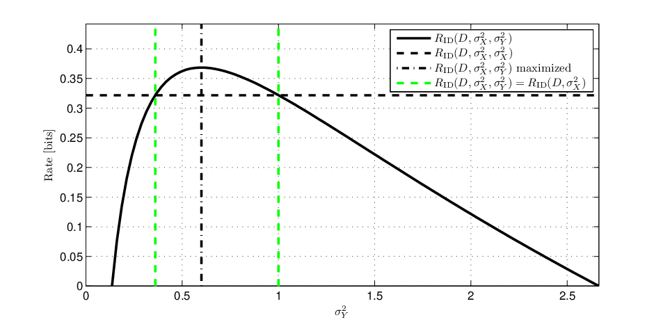
Refer to caption
Fig. 2: The identification rate RID​(D,σX2,σY2):=RID​(D,N⁡(μ,σX2),N⁡(μ,σY2))R_{\mathrm{ID}}(D,\sigma_{X}^{2},\sigma_{Y}^{2}):=R_{\mathrm{ID}}(D,N(\mu,\sigma_{X}^{2}),N(\mu,\sigma_{Y}^{2})) for different values of σY2\sigma_{Y}^{2}. Here σX2=1\sigma_{X}^{2}=1 and D=0.4D=0.4.

As an immediate corollary to Theorem 1, we obtain the following concise result for the symmetric case of PX=PY=N⁡(μ,σ2)P_{X}=P_{Y}=N(\mu,\sigma^{2}).

Corollary 1

If PX=PY=N⁡(μ,σ2)P_{X}=P_{Y}=N(\mu,\sigma^{2}), then

RID​(D,PX,PY)={log⁡(2​σ22​σ2−D)for 0≤D<2​σ2∞for D≥2​σ2.\displaystyle R_{\mathrm{ID}}(D,P_{X},P_{Y})=\left\{\begin{array}[]{ll}\log\left(\frac{2\sigma^{2}}{2\sigma^{2}-D}\right)&\mbox{for $0\leq D<2\sigma^{2}$}\\ \infty&\mbox{for $D\geq 2\sigma^{2}$}.\end{array}\right.

We remark that (1) is reminiscent of the Gaussian rate distortion function R⁡(D)=[12​log⁡σ2D]+R(D)=\left[\frac{1}{2}\log\frac{\sigma^{2}}{D}\right]^{+} (cf. [17]). The identification rate RID​(D,N⁡(μ,σ2),N⁡(μ,σ2))R_{\mathrm{ID}}(D,N(\mu,\sigma^{2}),N(\mu,\sigma^{2})) and rate distortion function R⁡(D)R(D) for a Gaussian source are plotted in Fig. 3, and as

Refer to caption
Fig. 3: The identification rate RID​(D):=RID​(D,N⁡(μ,σ2),N⁡(μ,σ2))R_{\mathrm{ID}}(D):=R_{\mathrm{ID}}(D,N(\mu,\sigma^{2}),N(\mu,\sigma^{2})) and the rate distortion function R⁡(D)R(D) for a Gaussian source with variance σ2\sigma^{2}.

seen in the figure, R⁡(D)R(D) is monotonically decreasing in DD, while (1) is monotone increasing. This can be intuitively explained by thinking of the compression scheme as a quantizer, where all the 𝐱\mathbf{x} sequences mapped to the same i∈{1,2,…,2n​R}i\in\{1,2,\dots,2^{nR}\} define a quantization cell. Since the scheme must answer 𝚖𝚊𝚢𝚋𝚎\mathtt{maybe} for all sequences 𝐲\mathbf{y} similar to 𝐱\mathbf{x}, it therefore has to answer 𝚖𝚊𝚢𝚋𝚎\mathtt{maybe} for all 𝐲\mathbf{y} in the DD-expansion of the quantization cell (all sequences that are at distance DD from any point in the cell). The probability of 𝚖𝚊𝚢𝚋𝚎\mathtt{maybe} is, therefore, the probability that 𝐘\mathbf{Y} falls in the expanded cell, and this probability increases as either DD grows, or as the size of the quantization cell itself grows (i.e. the rate decreases).

III-B The Identification Exponent for Gaussian Sources

Having established the identification rate for Gaussian sources, we now turn our attention to the identification exponent. In order to simplify the notation for the identification exponents, we define the following functions

𝐄Z​(ρ)\displaystyle\mathbf{E}_{Z}(\rho) ≜12​ln⁡2​(ρ−1−ln⁡ρ)\displaystyle\triangleq\frac{1}{2\ln 2}(\rho-1-\ln\rho) (19)
℘⁡(R,D,z1,z2)\displaystyle\wp(R,D,z_{1},z_{2}) ≜−log⁡sin⁡min⁡[π2,(arcsin⁡(2−R)+arccos⁡z1+z2−D2​z1​z2)].\displaystyle\triangleq-\log\sin\min\left[\tfrac{\pi}{2},\left(\arcsin\left(2^{-R}\right)+\arccos\frac{z_{1}+z_{2}-D}{2\sqrt{z_{1}z_{2}}}\right)\right]. (20)
Theorem 2

Let PX=N⁡(μ,σX2)P_{X}=N(\mu,\sigma_{X}^{2}) and PY=N⁡(μ,σY2)P_{Y}=N(\mu,\sigma_{Y}^{2}). For any fixed rate R>RID​(D,PX,PY)R>R_{\mathrm{ID}}(D,P_{X},P_{Y}),

𝐄ID​(R,D,PX,PY)=\displaystyle\mathbf{E}_{\mathrm{ID}}(R,D,P_{X},P_{Y})= minρX,ρY⁡𝐄Z​(ρX)+𝐄Z​(ρY)+℘⁡(R,D,ρX​σX2,ρY​σY2),\displaystyle\min_{\rho_{X},\rho_{Y}}\ \mathbf{E}_{Z}(\rho_{X})+\mathbf{E}_{Z}(\rho_{Y})+\wp(R,D,{\rho_{X}\sigma_{X}^{2}},{\rho_{Y}\sigma_{Y}^{2}}), (21)

where the minimization is over all ρX,ρY>0\rho_{X},\rho_{Y}>0 satisfying

|ρX​σX2−ρY​σY2|<D,\displaystyle\left|\sqrt{\rho_{X}\sigma_{X}^{2}}-\sqrt{\rho_{Y}\sigma_{Y}^{2}}\right|<\sqrt{D}, ρX​σX2+ρY​σY2≥D.\displaystyle\rho_{X}\sigma_{X}^{2}+\rho_{Y}\sigma_{Y}^{2}\geq D. (22)
Remark 1

We note that, for PX=N⁡(μ,σX2)P_{X}=N(\mu,\sigma_{X}^{2}) and PY=N⁡(μ,σY2)P_{Y}=N(\mu,\sigma_{Y}^{2}), the exponent 𝐄ID​(R,D,PX,PY)\mathbf{E}_{\mathrm{ID}}(R,D,P_{X},P_{Y}) is strictly positive for R>RID​(D,PX,PY)R>R_{\mathrm{ID}}(D,P_{X},P_{Y}), and is equal to zero at R=RID​(D,PX,PY)R=R_{\mathrm{ID}}(D,P_{X},P_{Y}). Therefore, the direct part of Theorem 1 is implied by Theorem 2. However, the converse part of Theorem 1 is not implied by Theorem 2, as the latter does not exclude the possibility that the probability of 𝚖𝚊𝚢𝚋𝚎\mathtt{maybe} can be made to vanish with a sub-exponential decay rate when the exponent is equal to zero.

In light of Theorem 2, it is instructive to revisit the relationship between false-positive and 𝚖𝚊𝚢𝚋𝚎\mathtt{maybe} probabilities specified in (13). To this end, consider the setting where PX=N⁡(μ,σX2)P_{X}=N(\mu,\sigma_{X}^{2}), PY=N⁡(μ,σY2)P_{Y}=N(\mu,\sigma_{Y}^{2}), and D≤σX2+σY2D\leq\sigma_{X}^{2}+\sigma_{Y}^{2}. In this case, the random variable 1n⁡(σX2+σY2)​‖𝐗−𝐘‖2\frac{1}{n(\sigma_{X}^{2}+\sigma_{Y}^{2})}\|\mathbf{X}-\mathbf{Y}\|^{2} has a chi-squared distribution with nn degrees of freedom. Therefore, it follows by Cramer’s Theorem (cf. [22, Theorem 2.2.3]) that

limn→∞−1nlogPr{d(𝐗,𝐘)≤D}\displaystyle\lim_{n\rightarrow\infty}-\frac{1}{n}\log\Pr\left\{d(\mathbf{X},\mathbf{Y})\leq D\right\} =𝐄Z​(DσX2+σY2).\displaystyle=\mathbf{E}_{Z}\left(\frac{D}{\sigma_{X}^{2}+\sigma_{Y}^{2}}\right). (23)

In this setting, it is a straightforward algebraic exercise to see that

𝐄ID​(R,D,PX,PY)<𝐄Z​(DσX2+σY2)\displaystyle\mathbf{E}_{\mathrm{ID}}(R,D,P_{X},P_{Y})<\mathbf{E}_{Z}\left(\frac{D}{\sigma_{X}^{2}+\sigma_{Y}^{2}}\right) (24)

for R<∞R<\infty by putting

ρX=σX2​D+σY2​(σX2+σY2)(σX2+σY2)2,\displaystyle\rho_{X}=\frac{\sigma_{X}^{2}D+\sigma_{Y}^{2}(\sigma_{X}^{2}+\sigma_{Y}^{2})}{(\sigma_{X}^{2}+\sigma_{Y}^{2})^{2}}, ρY=σY2​D+σX2​(σX2+σY2)(σX2+σY2)2\displaystyle\rho_{Y}=\frac{\sigma_{Y}^{2}D+\sigma_{X}^{2}(\sigma_{X}^{2}+\sigma_{Y}^{2})}{(\sigma_{X}^{2}+\sigma_{Y}^{2})^{2}} (25)

in (21). Therefore, 𝐄ID​(R,D,PX,PY)\mathbf{E}_{\mathrm{ID}}(R,D,P_{X},P_{Y}) also precisely characterizes the best-possible exponent corresponding to the probability of a false positive event in this setting due to the relation (13).

In the case where PX=PY=N⁡(μ,σ2)P_{X}=P_{Y}=N(\mu,\sigma^{2}), the symmetry in (21) can be exploited to yield the following corollary.

Corollary 2

Let PX=PY=N⁡(μ,σ2)P_{X}=P_{Y}=N(\mu,\sigma^{2}). For any fixed rate R>RID​(D,PX,PY)R>R_{\mathrm{ID}}(D,P_{X},P_{Y}),

𝐄ID​(R,D,PX,PY)=minρ⁡2​𝐄Z​(ρ)+℘⁡(R,D,ρ​σ2,ρ​σ2),\displaystyle\mathbf{E}_{\mathrm{ID}}(R,D,P_{X},P_{Y})=\min_{\rho}~2\mathbf{E}_{Z}(\rho)+\wp(R,D,{\rho\sigma^{2}},{\rho\sigma^{2}}), (26)

where the minimization is over all ρ\rho satisfying

2​σ2≥2​ρ​σ2≥D.\displaystyle 2\sigma^{2}\geq 2\rho\sigma^{2}\geq D. (27)

A formal proof is given in Section IV. The identification exponent (26) for the case of D/σ2=1.5D/\sigma^{2}=1.5 is illustrated in Fig. 4.

Refer to caption
Fig. 4: Plot of 𝐄ID​(R):=𝐄ID​(R,D,N⁡(μ,σ2),N⁡(μ,σ2))\mathbf{E}_{\mathrm{ID}}(R):=\mathbf{E}_{\mathrm{ID}}(R,D,N(\mu,\sigma^{2}),N(\mu,\sigma^{2})) for D/σ2=1.5D/\sigma^{2}=1.5. In this case, RID​(D,N⁡(μ,σ2),N⁡(μ,σ2))=2R_{\mathrm{ID}}(D,N(\mu,\sigma^{2}),N(\mu,\sigma^{2}))=2 bits per symbol.

Before proceeding, we briefly note that the identification exponent 𝐄ID​(R,D,PX,PY)\mathbf{E}_{\mathrm{ID}}(R,D,P_{X},P_{Y}) can sometimes be strictly positive at R→0R\rightarrow 0 33 3 Note that whenever RR is equal to zero, the probability of 𝚖𝚊𝚢𝚋𝚎\mathtt{maybe} is equal to 11 (unless the supports of PXP_{X} and PYP_{Y} are disjoint in a way making any two sequences 𝐱\mathbf{x} and 𝐲\mathbf{y} dissimilar, making the problem degenerate).. For instance, if

|1n​𝔼​‖𝐗‖−1n​𝔼​‖𝐘‖|>D+ϵ\displaystyle\left|\frac{1}{\sqrt{n}}\mathbb{E}\|\mathbf{X}\|-\frac{1}{\sqrt{n}}\mathbb{E}\|\mathbf{Y}\|\right|>\sqrt{D}+\epsilon (28)

for some ϵ>0\epsilon>0, then the signature T⁡(𝐗)T(\mathbf{X}) can simply indicate whether |1n​‖𝐗‖−1n​𝔼​‖𝐗‖|>ϵ/2\left|\frac{1}{\sqrt{n}}\|\mathbf{X}\|-\frac{1}{\sqrt{n}}\mathbb{E}\|\mathbf{X}\|\right|>\epsilon/2, requiring rate R=1/nR=1/n. Then, the query function gg returns 𝚖𝚊𝚢𝚋𝚎\mathtt{maybe} only if

|1n​‖𝐗‖−1n​𝔼​‖𝐗‖|>ϵ/2, or\displaystyle\left|\frac{1}{\sqrt{n}}\|\mathbf{X}\|-\frac{1}{\sqrt{n}}\mathbb{E}\|\mathbf{X}\|\right|>\epsilon/2,\mbox{~or} (29)
|1n​‖𝐘‖−1n​𝔼​‖𝐘‖|>ϵ/2.\displaystyle\left|\frac{1}{\sqrt{n}}\|\mathbf{Y}\|-\frac{1}{\sqrt{n}}\mathbb{E}\|\mathbf{Y}\|\right|>\epsilon/2. (30)

If neither (29) nor (30) occur, then it is readily verified that d⁡(𝐗,𝐘)>Dd(\mathbf{X},\mathbf{Y})>D using the triangle inequality. Whenever the random variables X2X^{2} and Y2Y^{2} satisfy a large deviations principle (as in the Gaussian case, and for many other distributions, cf. [22]), we see that gg returns 𝚖𝚊𝚢𝚋𝚎\mathtt{maybe} with probability exponentially decaying in nn, and we can conclude that limR→0+𝐄ID​(R,D,PX,PY)>0\lim_{R\rightarrow 0^{+}}\mathbf{E}_{\mathrm{ID}}(R,D,P_{X},P_{Y})>0. If this is indeed the case, then it also follows that RID​(D,PX,PY)=0R_{\mathrm{ID}}(D,P_{X},P_{Y})=0 by definition. Though this discussion applies for arbitrary distributions PX,PYP_{X},P_{Y}, this latter point is concretely reflected in Theorems 1 and 2 for the case where D≤(σX−σY)2D\leq(\sigma_{X}-\sigma_{Y})^{2}.

III-C Upper Bounds on the Identification Rate

In the previous two subsections, we focused our attention primarily to the case where PXP_{X} and PYP_{Y} were Gaussian distributions. In the sequel, we consider more general distributions and show that Gaussian PX,PYP_{X},P_{Y} constitute an extremal case in terms of the identification rate.

Theorem 3

Suppose PXP_{X} and PYP_{Y} are distributions with finite second moments σX2\sigma_{X}^{2} and σY2\sigma_{Y}^{2}, respectively. Then

RID​(D,PX,PY)≤R¯ID​(D,PX,PY)≜infPX^|XI⁡(X,X^),\displaystyle R_{\mathrm{ID}}(D,P_{X},P_{Y})\leq\overline{R}_{\mathrm{ID}}(D,P_{X},P_{Y})\triangleq\inf_{P_{\hat{X}|X}}I(X;\hat{X}), (31)

where the infimum is taken over all conditional distributions PX^|XP_{\hat{X}|X} satisfying

𝔼⁡[(σXσY​Y−X^)2]≥𝔼⁡[(σYσX​X−X^)2]+D−(σX−σY)2\displaystyle\sqrt{\mathbb{E}\left[\left(\sqrt{\frac{\sigma_{X}}{\sigma_{Y}}}Y-\hat{X}\right)^{2}\right]}\geq\sqrt{\mathbb{E}\left[\left(\sqrt{\frac{\sigma_{Y}}{\sigma_{X}}}X-\hat{X}\right)^{2}\right]}+\sqrt{D-(\sigma_{X}-\sigma_{Y})^{2}} (32)

for (Y,X,X^)∼PY​(y)​PX​(x)​PX^|X​(x^|x)(Y,X,\hat{X})\sim P_{Y}(y)P_{X}(x)P_{\hat{X}|X}(\hat{x}|x). Moreover,

𝐄ID​(R,D,PX,PY)>0\displaystyle\mathbf{E}_{\mathrm{ID}}(R,D,P_{X},P_{Y})>0 (33)

for any R>R¯ID​(D,PX,PY)R>\overline{R}_{\mathrm{ID}}(D,P_{X},P_{Y}).

Remark 2

Note that Theorem 3 does not require PXP_{X} and PYP_{Y} to have identical means.

Remark 3

Also note, that the achievability result and the proof technique carry over to general distortion criteria satisfying the triangle inequality. We omit the details as the focus of this paper is on the quadratic similarity criterion.

For general source distributions PX,PYP_{X},P_{Y}, we lack a matching lower bound on RID​(D,PX,PY)R_{\mathrm{ID}}(D,P_{X},P_{Y}). However, such a converse was proved in the Gaussian setting (see Theorem 1). The key ingredient in the proof of Theorem 1 is the isoperimetric inequality on the surface of a hypersphere – the set on which the probability of a high dimensional Gaussian random vector concentrates (see Section IV for details). In general, precise isoperimetric inequalities are unknown and therefore establishing a general converse appears to be extremely difficult.

In spite of this, an application of Theorem 3 reveals the interesting fact that Gaussian PXP_{X} and PYP_{Y} correspond to sources which are “most difficult” to compress for queries. This is analogous to the setting of classical lossy compression, where the Gaussian source requires the maximum rate for compression subject to a quadratic distortion constraint. Formally,

Theorem 4

Suppose PXP_{X} and PYP_{Y} have identical means and finite variances σX2\sigma_{X}^{2} and σY2\sigma_{Y}^{2}, respectively. Then

RID​(D,PX,PY)≤RID​(D,N⁡(0,σX2),N⁡(0,σY2)).\displaystyle R_{\mathrm{ID}}(D,P_{X},P_{Y})\leq R_{\mathrm{ID}}(D,N(0,\sigma_{X}^{2}),N(0,\sigma_{Y}^{2})). (34)

In particular, Gaussian PXP_{X} and PYP_{Y} demand the largest identification rate for given variances.

III-D Robust Identification Schemes

In addition to the extremal property of Gaussian sources described in Theorem 4, there exists a sequence of rate-RR identification schemes {T(n),g(n)}n→∞\{T^{(n)},g^{(n)}\}_{n\rightarrow\infty}, where (T(n),g(n))(T^{(n)},g^{(n)}) denotes a blocklength-nn identification scheme, designed for Gaussian sources which are robust in the following sense. Using the construction described in the achievability proof of Theorem 1, we can construct a sequence of DD-admissible, rate-RR schemes {T(n),g(n)}n→∞\{T^{(n)},g^{(n)}\}_{n\rightarrow\infty} which satisfy

limn→∞Pr{g(n)(T(n)(𝐗),𝐘)=𝚖𝚊𝚢𝚋𝚎}=0\displaystyle\lim_{n\rightarrow\infty}\Pr\left\{g^{(n)}\left(T^{(n)}(\mathbf{X}),\mathbf{Y}\right)=\mathtt{maybe}\right\}=0 (35)

when 𝐗,𝐘∼∏i=1nPX​(xi)​PY​(yi)\mathbf{X},\mathbf{Y}\sim\prod_{i=1}^{n}P_{X}(x_{i})P_{Y}(y_{i}), PX=N⁡(0,σX2)P_{X}=N(0,\sigma_{X}^{2}), PY=N⁡(0,σY2)P_{Y}=N(0,\sigma_{Y}^{2}) and

R>RID​(D,N⁡(0,σX2),N⁡(0,σY2)).\displaystyle R>R_{\mathrm{ID}}\left(D,N(0,\sigma_{X}^{2}),N(0,\sigma_{Y}^{2})\right). (36)

It turns out that this particular sequence {T(n),g(n)}n→∞\{T^{(n)},g^{(n)}\}_{n\rightarrow\infty} is robust to the source distributions in the sense that we also have

limn→∞Pr{g(n)(T(n)(𝐗~),𝐘~)=𝚖𝚊𝚢𝚋𝚎}=0\displaystyle\lim_{n\rightarrow\infty}\Pr\left\{g^{(n)}\left(T^{(n)}(\tilde{\mathbf{X}}),\tilde{\mathbf{Y}}\right)=\mathtt{maybe}\right\}=0 (37)

when 𝐗~,𝐘~∼∏i=1nPX~​(x~i)​PY~​(y~i)\tilde{\mathbf{X}},\tilde{\mathbf{Y}}\sim\prod_{i=1}^{n}P_{\tilde{X}}(\tilde{x}_{i})P_{\tilde{Y}}(\tilde{y}_{i}), and PX~P_{\tilde{X}}, PY~P_{\tilde{Y}} are zero-mean distributions with variances σX2\sigma_{X}^{2} and σY2\sigma_{Y}^{2}, respectively. Moreover, the sequence {T(n),g(n)}n→∞\{T^{(n)},g^{(n)}\}_{n\rightarrow\infty} continues to be DD-admissible for the sources 𝐗~,𝐘~\tilde{\mathbf{X}},\tilde{\mathbf{Y}}. Thus, roughly speaking, a scheme (T,g)(T,g) which is “good” for Gaussian sources 𝐗,𝐘\mathbf{X},\mathbf{Y} can be expected to perform well for arbitrary sources 𝐗~,𝐘~\tilde{\mathbf{X}},\tilde{\mathbf{Y}}, provided the respective variances match their Gaussian counterparts and the blocklength nn is large. The proof of this robustness property is given in Section IV-F.

IV Proofs

In this section, we prove each of the main results. Proofs are organized by subsection. We begin with a primer on the key geometric ideas that are used throughout the proofs.

IV-A Geometric Preliminaries

For the proofs we require the following definitions related to nn-dimensional Euclidean geometry.

For r>0,𝐮∈ℝnr>0,\mathbf{u}\in\mathds{R}^{n}, let BALLr​(𝐮)⊆ℝn\mathrm{BALL}_{r}(\mathbf{u})\subseteq\mathds{R}^{n} denote the ball with radius rr centered at 𝐮\mathbf{u}:

BALLr​(𝐮)≜{𝐱∈ℝn:‖𝐱−𝐮‖≤r}.\mathrm{BALL}_{r}(\mathbf{u})\triangleq\left\{\mathbf{x}\in\mathds{R}^{n}:\|\mathbf{x}-\mathbf{u}\|\leq r\right\}. (38)

BALLr​(𝟎)\mathrm{BALL}_{r}(\mathbf{0}) will be denoted BALLr\mathrm{BALL}_{r}.

Denote by Sr⊆ℝnS_{r}\subseteq\mathds{R}^{n} the spherical shell with radius rr centered at the origin:

Sr≜{𝐱∈ℝn:‖𝐱‖=r}.S_{r}\triangleq\left\{\mathbf{x}\in\mathds{R}^{n}:\|\mathbf{x}\|=r\right\}. (39)

For any two vectors 𝐱1,𝐱2∈ℝn∖{𝟎}\mathbf{x}_{1},\mathbf{x}_{2}\in\mathds{R}^{n}\setminus\{\mathbf{0}\}, the angle between them shall be denoted by

∠⁡(𝐱1,𝐱2)≜arccos⁡(𝐱1T​𝐱2‖𝐱1‖​‖𝐱2‖)∈[0,π].\angle(\mathbf{x}_{1},\mathbf{x}_{2})\triangleq\arccos\left(\frac{\mathbf{x}_{1}^{T}\mathbf{x}_{2}}{\|\mathbf{x}_{1}\|\|\mathbf{x}_{2}\|}\right)\in[0,\pi]. (40)

For θ∈[0,π]\theta\in[0,\pi] and a point 𝐮∈ℝn∖{𝟎}\mathbf{u}\in\mathds{R}^{n}\setminus\{\mathbf{0}\}, define the cone with half angle θ\theta and axis going through 𝐮\mathbf{u}:

CONE⁡(𝐮,θ)≜{𝐱∈ℝn:∠⁡(𝐮,𝐱)≤θ}.\mathrm{CONE}(\mathbf{u},\theta)\triangleq\left\{\mathbf{x}\in\mathds{R}^{n}:\angle(\mathbf{u},\mathbf{x})\leq\theta\right\}. (41)

Note that CONE⁡(𝐮,0)\mathrm{CONE}(\mathbf{u},0) is the half-infinite line {α​𝐮:α>0}\{\alpha\mathbf{u}:\alpha>0\}, that CONE⁡(𝐮,π/2)\mathrm{CONE}(\mathbf{u},\pi/2) is the half-space containing 𝐮\mathbf{u} that is bordered by the hyperplane orthogonal to 𝐮\mathbf{u} which passes through the origin, and that CONE⁡(𝐮,π)\mathrm{CONE}(\mathbf{u},\pi) is the entire space ℝn\mathds{R}^{n}. Also, note that CONE⁡(𝐮1,θ)=CONE⁡(𝐮2,θ)\mathrm{CONE}(\mathbf{u}_{1},\theta)=\mathrm{CONE}(\mathbf{u}_{2},\theta) for any 𝐮1=λ​𝐮2\mathbf{u}_{1}=\lambda\mathbf{u}_{2}, λ>0\lambda>0.

For r>0,𝐮∈ℝn∖{𝟎}r>0,\mathbf{u}\in\mathds{R}^{n}\setminus\{\mathbf{0}\} and θ∈[0,π]\theta\in[0,\pi], denote by CAPr​(𝐮,θ)\mathrm{CAP}_{r}(\mathbf{u},\theta) the spherical cap:

CAPr​(𝐮,θ)≜Sr∩CONE⁡(𝐮,θ).\mathrm{CAP}_{r}(\mathbf{u},\theta)\triangleq S_{r}\cap\mathrm{CONE}(\mathbf{u},\theta). (42)

Let Ω⁡(θ)\Omega(\theta) denote the fraction of the (hyper-)surface area of SrS_{r} that is occupied by CAPr​(𝐮,θ)\mathrm{CAP}_{r}(\mathbf{u},\theta):

Ω⁡(θ)≜|CAPr​(𝐮,θ)||Sr|.\Omega(\theta)\triangleq\frac{|\mathrm{CAP}_{r}(\mathbf{u},\theta)|}{|S_{r}|}. (43)

Note that the value of Ω⁡(θ)\Omega(\theta) depends neither on rr nor on 𝐮\mathbf{u}. The following bounds on Ω⁡(θ)\Omega(\theta) will be useful:

Lemma 1

[23, Corrolary 3.2] For 0<θ<arccos⁡(1/n)<π20<\theta<\arccos(1/\sqrt{n})<\frac{\pi}{2}, we have

Ω⁡(θ)\displaystyle\Omega(\theta) <12​π​(n−1)⋅1cos⁡θ⋅sinn−1⁡θ,\displaystyle<\frac{1}{\sqrt{2\pi(n-1)}}\cdot\frac{1}{\cos\theta}\cdot\sin^{n-1}\theta, (44)
Ω⁡(θ)\displaystyle\Omega(\theta) >13​2​π​n⋅1cos⁡θ⋅sinn−1⁡θ.\displaystyle>\frac{1}{3\sqrt{2\pi n}}\cdot\frac{1}{\cos\theta}\cdot\sin^{n-1}\theta. (45)

For positive r1≤r2∈ℝr_{1}\leq r_{2}\in\mathds{R}, let Sr1,r2⊆ℝnS_{r_{1},r_{2}}\subseteq\mathds{R}^{n} be a spherical shell of inner radius r1r_{1} and outer radius r2r_{2}:

Sr1,r2≜{𝐱∈ℝn:r1≤‖𝐱‖≤r2}.S_{r_{1},r_{2}}\triangleq\left\{\mathbf{x}\in\mathds{R}^{n}:r_{1}\leq\|\mathbf{x}\|\leq r_{2}\right\}. (46)

For a given half-angle θ∈[0,π]\theta\in[0,\pi], define the (r1,r2)(r_{1},r_{2})-spherical cap with half-angle θ\theta and axis going through 𝐮\mathbf{u} as

CAPr1,r2​(𝐮,θ)\displaystyle\mathrm{CAP}_{r_{1},r_{2}}(\mathbf{u},\theta) ≜CONE⁡(𝐮,θ)∩Sr1,r2.\displaystyle\triangleq\mathrm{CONE}(\mathbf{u},\theta)\cap S_{r_{1},r_{2}}. (47)

For a set A⊆ℝnA\subseteq\mathds{R}^{n} and D>0D>0, the DD-expansion of AA, denoted ΓD​(A)\Gamma^{D}(A) is defined as

ΓD​(A)\displaystyle\Gamma^{D}(A) ≜{𝐲∈ℝn:∃𝐱∈Ad⁡(𝐱,𝐲)≤D}\displaystyle\triangleq\{\mathbf{y}\in\mathds{R}^{n}:\exists_{\mathbf{x}\in A}d(\mathbf{x},\mathbf{y})\leq D\} (48)
=A+BALLn​D,\displaystyle=A+\mathrm{BALL}_{\sqrt{nD}}, (49)

where we have used ++ to denote the Minkowski sum.

IV-B Codes that cover a spherical shell

Definition 4

Let Sr⊆ℝnS_{r}\subseteq\mathds{R}^{n} be the spherical shell with radius rr. We say that a set of points 𝒞={𝐮1,…,𝐮m:𝐮i∈ℝn}\mathcal{C}=\{\mathbf{u}_{1},\dots,\mathbf{u}_{m}:\mathbf{u}_{i}\in\mathds{R}^{n}\} is a code that DD-covers SrS_{r} if

Sr⊆⋃𝐮∈𝒞BALLn​D​(𝐮).\displaystyle S_{r}\subseteq\bigcup_{\mathbf{u}\in\mathcal{C}}\mathrm{BALL}_{\sqrt{nD}}(\mathbf{u}). (50)

The rate of 𝒞\mathcal{C} is defined as 1n​log⁡m\frac{1}{n}\log m.

When not explicitly stated, the ambient dimension nn of the code 𝒞\mathcal{C} will be clear from context.

Lemma 2 (Following [24])

Fix σ2>0\sigma^{2}>0 and the dimension nn. For any 0<D0<σ20<D_{0}<\sigma^{2}, there exists a code 𝒞\mathcal{C} that D0D_{0}-covers Sn​σ2S_{\sqrt{n\sigma^{2}}} with rate

R0=1n​log⁡|𝒞|≤12​log⁡σ2D0+O⁡(log⁡nn).R_{0}=\frac{1}{n}\log|\mathcal{C}|\leq\frac{1}{2}\log\frac{\sigma^{2}}{D_{0}}+O\left(\frac{\log n}{n}\right). (51)

Moreover, for all 𝐮∈𝒞\mathbf{u}\in\mathcal{C}, we have ‖𝐮‖=n⁡(σ2−D0)\|\mathbf{u}\|=\sqrt{n(\sigma^{2}-D_{0})}, and

CAPn​σ2​(𝐮,θ0)=Sn​σ2∩BALLn​D0​(𝐮),\displaystyle\mathrm{CAP}_{\sqrt{n\sigma^{2}}}(\mathbf{u},\theta_{0})=S_{\sqrt{n\sigma^{2}}}\cap\mathrm{BALL}_{\sqrt{nD_{0}}}(\mathbf{u}), (52)

where

θ0≜arcsin⁡(D0/σ2)<π2.\theta_{0}\triangleq\arcsin(\sqrt{D_{0}/\sigma^{2}})<\frac{\pi}{2}. (53)
Proof:

Appendix A.∎

It is no surprise that the term 12​log⁡σ2D0\frac{1}{2}\log\frac{\sigma^{2}}{D_{0}} appearing in (51) is identical to the rate-distortion function for the Gaussian source with variance σ2\sigma^{2} evaluated at distortion-level D0D_{0}. We could have therefore used any standard (random code-like) construction. However, using Lemma 2 will be more convenient for our purposes since each point in SrS_{r} is guaranteed to be covered, and hence we do not need to account for another error event. This fact will make the subsequent proofs more straightforward.

IV-C Identification Rate

The proof of Theorem 1 is somewhat lengthy, so we first give the key ideas here before moving onto the formal details.

The proof of the theorem relies on the fact that a high-dimensional Gaussian random vector – with independent entries having zero mean and variance σX2\sigma_{X}^{2} – concentrates near a thin hyper-spherical shell of radius r0≜n​σX2r_{0}\triangleq\sqrt{n\sigma_{X}^{2}}, which we call the typical sphere. The signature assignment constructed in the direct part of the proof quantizes the surface of the typical sphere into regions roughly described by spherical caps. The query function gg, knowing which cap 𝐗\mathbf{X} lies in from the received signature, returns 𝚖𝚊𝚢𝚋𝚎\mathtt{maybe} only if 𝐘\mathbf{Y} lies within Euclidean distance D\sqrt{D} of the cap in which 𝐗\mathbf{X} lies. Thus, the goal in the direct part is to show that, for sufficiently large rate RR, the probability 𝐘\mathbf{Y} falls into the ΓD\Gamma^{D}-expansion of any given cap is vanishing.

The key ingredient in proving the converse is the isoperimetric inequality on the surface of the hypersphere, known as Levy’s lemma (see e.g. [25, Theorem 1.1]). In a nutshell, we apply Levy’s lemma to prove that any given identification system (T,g)(T,g) requires a rate that is essentially as large as an identification system that uniquely assigns caps on the typical sphere to signatures (as is done by the achievability scheme). The apparent need for a refined isoperimetric inequality to prove the converse distinguishes our problem from the class of standard rate-distortion problems.

Proof:

Before beginning the proof, we first note that it is sufficient to consider DD in the interval (σX−σY)2<D<σX2+σY2(\sigma_{X}-\sigma_{Y})^{2}<D<\sigma_{X}^{2}+\sigma_{Y}^{2}. The claims that RID​(D,PX,PY)=0R_{\mathrm{ID}}(D,P_{X},P_{Y})=0 for D≤(σX−σY)2D\leq(\sigma_{X}-\sigma_{Y})^{2}, and RID​(D,PX,PY)=∞R_{\mathrm{ID}}(D,P_{X},P_{Y})=\infty for D≥σX2+σY2D\geq\sigma_{X}^{2}+\sigma_{Y}^{2} then follow from monotonicity of RID​(D,PX,PY)R_{\mathrm{ID}}(D,P_{X},P_{Y}) in DD.

Direct Part: Fix a small ϵ>0\epsilon>0, and define rX≜n​σX2r_{X}\triangleq\sqrt{n\sigma_{X}^{2}} (i.e., the radius of the typical sphere). Let DD be a desired similarity threshold in the interval (σX−σY)2<D<σX2+σY2(\sigma_{X}-\sigma_{Y})^{2}<D<\sigma_{X}^{2}+\sigma_{Y}^{2}, and let η>0\eta>0 be sufficiently small so that

(1−ϵ)​[σX2+σY2−D2​σX​σY]2<[σX2+σY2−2​η−D2​(σX2+η)​(σY2+η)]2.\displaystyle(1-\epsilon)\left[\frac{\sigma_{X}^{2}+\sigma_{Y}^{2}-D}{2\sigma_{X}\sigma_{Y}}\right]^{2}<\left[\frac{\sigma_{X}^{2}+\sigma_{Y}^{2}-2\eta-D}{2\sqrt{(\sigma_{X}^{2}+\eta)(\sigma_{Y}^{2}+\eta)}}\right]^{2}. (54)

Next, define a constant D0D_{0} satisfying

(1−ϵ)​σX2​[σX2+σY2−2​η−D2​(σX2+η)​(σY2+η)]2<D0<σX2​[σX2+σY2−2​η−D2​(σX2+η)​(σY2+η)]2.\displaystyle(1-\epsilon)\sigma_{X}^{2}\left[\frac{\sigma_{X}^{2}+\sigma_{Y}^{2}-2\eta-D}{2\sqrt{(\sigma_{X}^{2}+\eta)(\sigma_{Y}^{2}+\eta)}}\right]^{2}<D_{0}<\sigma_{X}^{2}\left[\frac{\sigma_{X}^{2}+\sigma_{Y}^{2}-2\eta-D}{2\sqrt{(\sigma_{X}^{2}+\eta)(\sigma_{Y}^{2}+\eta)}}\right]^{2}. (55)

The motivation behind the choices of η\eta and D0D_{0} satisfying (54) and (55) will become clear as the proof proceeds.

By our assumption that D>(σX−σY)2D>(\sigma_{X}-\sigma_{Y})^{2}, it follows that 0<D0<σX20<D_{0}<\sigma_{X}^{2}. By Lemma 2, there exists a code 𝒞\mathcal{C} which D0D_{0}-covers SrXS_{r_{X}} with rate R0R_{0} bounded by

R0≤12​log⁡σX2D0+O⁡(log⁡nn).\displaystyle R_{0}\leq\frac{1}{2}\log\frac{\sigma_{X}^{2}}{D_{0}}+O\left(\frac{\log n}{n}\right). (56)

Let T0:SrX→𝒞T_{0}:S_{r_{X}}\rightarrow\mathcal{C} be the quantization operation defined by

T0​(𝐱)=arg⁡min𝐮∈𝒞​‖𝐱−𝐮‖​ for 𝐱∈SrX.\displaystyle T_{0}(\mathbf{x})=\arg\min_{\mathbf{u}\in\mathcal{C}}\|\mathbf{x}-\mathbf{u}\|\mbox{~~for $\mathbf{x}\in S_{r_{X}}$.} (57)

That is, the function T0​(𝐱)T_{0}(\mathbf{x}) maps 𝐱∈SrX\mathbf{x}\in S_{r_{X}} to the closest reconstruction point 𝐮∈𝒞\mathbf{u}\in\mathcal{C}. Since 𝒞\mathcal{C} is a code that D0D_{0}-covers SrXS_{r_{X}}, it follows that

‖T0​(𝐱)−𝐱‖≤ρ0≜n​D0​ for all 𝐱∈SrX.\displaystyle\|T_{0}(\mathbf{x})-\mathbf{x}\|\leq\rho_{0}\triangleq\sqrt{nD_{0}}\mbox{~~for all $\mathbf{x}\in S_{r_{X}}$.} (58)

Denote the points in SrXS_{r_{X}} that are mapped to 𝐮\mathbf{u} by T0−1​(𝐮)T_{0}^{-1}(\mathbf{u}). With this notation, it follows by construction that

T0−1​(𝐮)⊆CAPrX​(𝐮,θ0),T_{0}^{-1}(\mathbf{u})\subseteq\mathrm{CAP}_{r_{X}}(\mathbf{u},\theta_{0}), (59)

where θ0≜arcsin⁡(D0/σX2)\theta_{0}\triangleq\arcsin(\sqrt{D_{0}/\sigma_{X}^{2}}) courtesy of Lemma 2. The set CAPrX​(𝐮,θ0)\mathrm{CAP}_{r_{X}}(\mathbf{u},\theta_{0}) is illustrated in Fig. 5.

Refer to caption r X θ 0 u ρ 0
Fig. 5: Illustration of a single cap CAPrX​(𝐮,θ0)\mathrm{CAP}_{r_{X}}(\mathbf{u},\theta_{0}) (denoted in grey).

Define SXtypS^{\mathrm{typ}}_{X} to be the set of all vectors 𝐱∈ℝn\mathbf{x}\in\mathds{R}^{n} s.t. σX2−η≤1n​‖𝐱‖2≤σX2+η\sigma_{X}^{2}-\eta\leq\frac{1}{n}\|\mathbf{x}\|^{2}\leq\sigma_{X}^{2}+\eta. In other words,

SXtyp≜Sr−,r+,S^{\mathrm{typ}}_{X}\triangleq S_{r^{-},r^{+}}, (60)

where r±≜n⁡(σX2±η)r^{\pm}\triangleq\sqrt{n(\sigma_{X}^{2}\pm\eta)}. Note that Pr{𝐗∉SXtyp}\Pr\{\mathbf{X}\notin S^{\mathrm{typ}}_{X}\} vanishes with nn (in fact, it vanishes exponentially), which motivates the notation SXtypS^{\mathrm{typ}}_{X}.

Next, we construct a mapping T:SXtyp→𝒞T:S^{\mathrm{typ}}_{X}\rightarrow\mathcal{C} defined as follows:

T⁡(𝐱)=T0​(𝐱⋅n​σX2‖𝐱‖).T(\mathbf{x})=T_{0}\left(\mathbf{x}\cdot\frac{\sqrt{n\sigma_{X}^{2}}}{\|\mathbf{x}\|}\right). (61)

Since T0−1​(𝐮)T_{0}^{-1}(\mathbf{u}) is contained in CAPrX​(𝐮,θ0)\mathrm{CAP}_{r_{X}}(\mathbf{u},\theta_{0}), we similarly have that the inverse map T−1T^{-1} satisfies

T−1​(𝐮)⊆CAPr−,r+​(𝐮,θ0).T^{-1}(\mathbf{u})\subseteq\mathrm{CAP}_{r^{-},r^{+}}(\mathbf{u},\theta_{0}). (62)

The signature assignment for our identification scheme for 𝐱∈SXtyp\mathbf{x}\in S^{\mathrm{typ}}_{X} shall be given by the function T⁡(⋅)T(\cdot) defined above. For 𝐱∉SXtyp\mathbf{x}\notin S^{\mathrm{typ}}_{X} we define T⁡(𝐱)=𝚎T(\mathbf{x})=\mathtt{e}, where 𝚎\mathtt{e} is an additional “erasure” symbol, denoting the fact that the signature does not convey any information about 𝐱\mathbf{x} in this case (and the decision function g⁡(⋅,⋅)g(\cdot,\cdot) must output 𝚖𝚊𝚢𝚋𝚎\mathtt{maybe}). Note that the additional rate incurred by the erasure symbol is negligible and we still have that the signature assignment’s rate RR is bounded by

R\displaystyle R =1n​log⁡(|𝒞|+1)\displaystyle=\frac{1}{n}\log\left(|\mathcal{C}|+1\right) (63)
≤12​log⁡σX2D0+O⁡(log⁡nn)\displaystyle\leq\frac{1}{2}\log\frac{\sigma_{X}^{2}}{D_{0}}+O\left(\frac{\log n}{n}\right) (64)
≤log⁡2​σX​σYσX2+σY2−D+log⁡11−ϵ+O⁡(log⁡nn),\displaystyle\leq\log\frac{2\sigma_{X}\sigma_{Y}}{\sigma_{X}^{2}+\sigma_{Y}^{2}-D}+\log\frac{1}{1-\epsilon}+O\left(\frac{\log n}{n}\right), (65)

where the final inequality follows from (54) and (55).

The query function g⁡(⋅,⋅)g(\cdot,\cdot) is defined to be the optimal one given the signature mapping T⁡(⋅)T(\cdot):

g⁡(t,𝐲)={𝚖𝚊𝚢𝚋𝚎If t=𝚎 or if ∃𝐱′∈T−1​(t)​ s.t. ​d​(𝐱′,𝐲)≤D𝚗𝚘otherwise.g(t,\mathbf{y})=\left\{\begin{array}[]{ll}\mathtt{maybe}&\hbox{If $t=\mathtt{e}$ or if $\exists\mathbf{x}^{\prime}\in T^{-1}(t)\mbox{ s.t. }d(\mathbf{x}^{\prime},\mathbf{y})\leq D$}\\ \mathtt{no}&\hbox{otherwise.}\end{array}\right. (66)

Using the shorthand notation

Pr{𝚖𝚊𝚢𝚋𝚎}≜Pr{g(T(𝐗),𝐘)=𝚖𝚊𝚢𝚋𝚎},\displaystyle\Pr\{\mathtt{maybe}\}\triangleq\Pr\{g(T(\mathbf{X}),\mathbf{Y})=\mathtt{maybe}\}, (67)

we analyze Pr⁡{𝚖𝚊𝚢𝚋𝚎}\Pr\{\mathtt{maybe}\} as follows. First, define a typical set for the 𝐘\mathbf{Y}-sequences:

SYtyp≜SrY−,rY+,S^{\mathrm{typ}}_{Y}\triangleq S_{r_{Y}^{-},r_{Y}^{+}}, (68)

where rY±≜n⁡(σY2±η)r_{Y}^{\pm}\triangleq\sqrt{n(\sigma_{Y}^{2}\pm\eta)}, and write

Pr⁡{𝚖𝚊𝚢𝚋𝚎}\displaystyle\Pr\{\mathtt{maybe}\} ≤Pr{𝚖𝚊𝚢𝚋𝚎|𝐗∈SXtyp,𝐘∈SYtyp}+Pr{𝐗∉SXtyp}+Pr{𝐘∉SYtyp}.\displaystyle\leq\Pr\{\mathtt{maybe}|\mathbf{X}\in S^{\mathrm{typ}}_{X},\mathbf{Y}\in S^{\mathrm{typ}}_{Y}\}+\Pr\{\mathbf{X}\notin S^{\mathrm{typ}}_{X}\}+\Pr\{\mathbf{Y}\notin S^{\mathrm{typ}}_{Y}\}. (69)

Note that the latter two terms in (69) vanish as nn grows large, thus we focus on bounding the first term. To this end, we require the following lemma.

Lemma 3

Let 𝒞\mathcal{C} and η\eta be as defined above. For any 𝐮∈𝒞\mathbf{u}\in\mathcal{C}, we have

ΓD​(T−1​(𝐮))∩SYtyp⊆CONE⁡(𝐮,θ′),\Gamma^{D}\left(T^{-1}(\mathbf{u})\right)\cap S^{\mathrm{typ}}_{Y}\subseteq\mathrm{CONE}(\mathbf{u},\theta^{\prime}), (70)

where

θ′≜θ0+θ1<π2,\theta^{\prime}\triangleq\theta_{0}+\theta_{1}<\frac{\pi}{2}, (71)

and the angles θ0\theta_{0} and θ1\theta_{1} are given by

θ0\displaystyle\theta_{0} ≜arcsin⁡(D0σX2)\displaystyle\triangleq\arcsin\left(\sqrt{\frac{D_{0}}{\sigma_{X}^{2}}}\right) (72)
θ1\displaystyle\theta_{1} ≜arccos⁡(σX2+σY2−2​η−D2​(σX2+η)​(σY2+η)).\displaystyle\triangleq\arccos\left(\frac{\sigma_{X}^{2}+\sigma_{Y}^{2}-2\eta-D}{2\sqrt{(\sigma_{X}^{2}+\eta)(\sigma_{Y}^{2}+\eta)}}\right). (73)
Proof:

Appendix B. ∎ Fig. 6 illustrates the claim in the lemma.

Refer to caption r X θ 0 r Y θ 1 ⁢ n D ⁢ n D S typ Y u S typ X
Fig. 6: Illustration for Lemma 3. The black region marks CAPr−,r+​(𝐮,θ0)\mathrm{CAP}_{r^{-},r^{+}}(\mathbf{u},\theta_{0}). The grey area denotes ΓD​(CAPr−,r+​(𝐮,θ0))\Gamma^{D}\left(\mathrm{CAP}_{r^{-},r^{+}}(\mathbf{u},\theta_{0})\right), and the dark grey region marks the intersection ΓD​(CAPr−,r+​(𝐮,θ0))∩SYtyp\Gamma^{D}\left(\mathrm{CAP}_{r^{-},r^{+}}(\mathbf{u},\theta_{0})\right)\cap S^{\mathrm{typ}}_{Y}.

Let θ′\theta^{\prime} be as defined in Lemma 3 above. We continue with

Pr{𝚖𝚊𝚢𝚋𝚎|𝐗∈SXtyp,𝐘∈SYtyp}\displaystyle\!\!\Pr\{\mathtt{maybe}|\mathbf{X}\in S^{\mathrm{typ}}_{X},\mathbf{Y}\in S^{\mathrm{typ}}_{Y}\} =(a)Pr{𝐘∈ΓD(T−1(T(𝐗)))|𝐗∈SXtyp,𝐘∈SYtyp}\displaystyle\overset{(a)}{=}\Pr\left\{\mathbf{Y}\in\Gamma^{D}\left(T^{-1}(T(\mathbf{X}))\right)|\mathbf{X}\in S^{\mathrm{typ}}_{X},\mathbf{Y}\in S^{\mathrm{typ}}_{Y}\right\}
≤(b)Pr{𝐘∈CONE(T(𝐗),θ′)|𝐗∈SXtyp,𝐘∈SYtyp}\displaystyle\overset{(b)}{\leq}\Pr\left\{\mathbf{Y}\in\mathrm{CONE}(T(\mathbf{X}),\theta^{\prime})|\mathbf{X}\in S^{\mathrm{typ}}_{X},\mathbf{Y}\in S^{\mathrm{typ}}_{Y}\right\}
=(c)​Ω​(θ′)\displaystyle\overset{(c)}{=}\Omega(\theta^{\prime})
≤(d)​12​π​(n−1)⋅1cos⁡θ′⋅sinn−1⁡θ′.\displaystyle\overset{(d)}{\leq}\frac{1}{\sqrt{2\pi(n-1)}}\cdot\frac{1}{\cos\theta^{\prime}}\cdot\sin^{n-1}\theta^{\prime}. (74)

Identity (a)(a) follows by definition of the query function g⁡(⋅,⋅)g(\cdot,\cdot). Inequality (b)(b) follows from Lemma 3. Equality (c)(c) follows since 𝐘\mathbf{Y} is uniformly distributed within each shell SrS_{r} of radius r>0r>0 (due to the spherical symmetry of the Gaussian distribution), and the probability of falling in a cap of a given half-angle θ′\theta^{\prime} is precisely the fraction of the surface that is occupied by the cap, Ω⁡(θ′)\Omega(\theta^{\prime}). Inequality (d)(d) follows since θ′≤arccos⁡(1/n)\theta^{\prime}\leq\arccos(1/\sqrt{n}) for sufficiently large nn, and therefore (44) applies.

Since θ′<π/2\theta^{\prime}<\pi/2, we have sin⁡θ′<1\sin\theta^{\prime}<1, and it therefore follows from (74) that the probability Pr{𝚖𝚊𝚢𝚋𝚎|𝐗∈Styp,𝐘∈SYtyp}\Pr\{\mathtt{maybe}|\mathbf{X}\in S^{\mathrm{typ}},\mathbf{Y}\in S^{\mathrm{typ}}_{Y}\} vanishes with nn. Thus, since ϵ\epsilon was arbitrary, recalling (65) completes the direct part of the proof.

Remark 4

The alert reader will observe that the direct part also follows from the direct part of Theorem 2. However, we have chosen to include an explicit proof here to introduce the notations and ideas crucial for proving Theorem 2.

Converse Part: Let η>0\eta>0 and define SXtypS^{\mathrm{typ}}_{X} as in (60). Let T:ℝn→{1,…,2n​R}T:\mathds{R}^{n}\rightarrow\{1,...,2^{nR}\} be a given signature function corresponding to a DD-admissible system (T,g)(T,g), and assume that

Pr{g(T(𝐗),𝐘)=𝚖𝚊𝚢𝚋𝚎}≤14\displaystyle\Pr\{g(T(\mathbf{X}),\mathbf{Y})=\mathtt{maybe}\}\leq\frac{1}{4} (75)

since we are only interested in DD-achievable rates RR. As before, we will use the shorthand notation Pr{𝚖𝚊𝚢𝚋𝚎}≜Pr{g(T(𝐗),𝐘)=𝚖𝚊𝚢𝚋𝚎}\Pr\{\mathtt{maybe}\}\triangleq\Pr\{g(T(\mathbf{X}),\mathbf{Y})=\mathtt{maybe}\} to simplify the presentation.

We shall restrict our attention to the typical sphere. To this end, define the mapping T~:SXtyp→{1,…,2n​R}\tilde{T}:S^{\mathrm{typ}}_{X}\rightarrow\{1,...,2^{nR}\}, where T~​(𝐱)=T​(𝐱)\tilde{T}(\mathbf{x})=T(\mathbf{x}) for 𝐱∈SXtyp\mathbf{x}\in S^{\mathrm{typ}}_{X}. Let T~−1​(⋅)\tilde{T}^{-1}(\cdot) denote the inverse mapping of T~​(⋅)\tilde{T}(\cdot), i.e.

T~−1​(i)\displaystyle\tilde{T}^{-1}(i) ≜{𝐱∈SXtyp:T⁡(𝐱)=i}\displaystyle\triangleq\{\mathbf{x}\in S^{\mathrm{typ}}_{X}:T(\mathbf{x})=i\} (76)
=T−1​(i)∩SXtyp.\displaystyle=T^{-1}(i)\cap S^{\mathrm{typ}}_{X}. (77)

Let pi≜Pr⁡{𝐗∈T~−1​(i)|𝐗∈SXtyp}p_{i}\triangleq\Pr\{\mathbf{X}\in\tilde{T}^{-1}(i)|\mathbf{X}\in S^{\mathrm{typ}}_{X}\}. Clearly, we have ∑i=12n​Rpi=1\sum_{i=1}^{2^{nR}}p_{i}=1. Define the set Ai⊆SrXA_{i}\subseteq S_{r_{X}} to be projection of T~−1​(i)\tilde{T}^{-1}(i) onto the sphere SrXS_{r_{X}}:

Ai={rX​𝐱‖𝐱‖:𝐱∈T~−1​(i)}A_{i}=\left\{r_{X}\frac{\mathbf{x}}{\|\mathbf{x}\|}:\mathbf{x}\in\tilde{T}^{-1}(i)\right\} (78)

Let αi\alpha_{i} denote the fraction of the surface area of SrXS_{r_{X}} that is occupied by AiA_{i}. By the spherical symmetry of the pdf of 𝐗\mathbf{X}, αi\alpha_{i} is also equal to the probability that the projection of 𝐗\mathbf{X} onto Sr0S_{r_{0}} lies in AiA_{i}. Therefore αi≥pi\alpha_{i}\geq p_{i}, with equality if and only if T~−1​(i)\tilde{T}^{-1}(i) is a thick cap with inner and outer radii r±≜n⁡(σX2±η)r^{\pm}\triangleq\sqrt{n(\sigma_{X}^{2}\pm\eta)}.

Let D′≜(D+σX2−η−σX2)2<DD^{\prime}\triangleq(\sqrt{D}+\sqrt{\sigma_{X}^{2}-\eta}-\sqrt{\sigma_{X}^{2}})^{2}<D. It can easily be verified that

ΓD′​(Ai)⊆ΓD​(T~−1​(i)).\Gamma^{D^{\prime}}\left(A_{i}\right)\subseteq\Gamma^{D}\left(\tilde{T}^{-1}(i)\right). (79)

Now let D′′≜(D′+σY2−η−σY2)2D^{\prime\prime}\triangleq(\sqrt{D^{\prime}}+\sqrt{\sigma_{Y}^{2}-\eta}-\sqrt{\sigma_{Y}^{2}})^{2}, and let the set BiB_{i} denote the D′′D^{\prime\prime}-expansion of AiA_{i}, restricted to the sphere SrYS_{r_{Y}}, i.e.

Bi≜ΓD′′​(Ai)∩SrY.B_{i}\triangleq\Gamma^{D^{\prime\prime}}\left(A_{i}\right)\cap S_{r_{Y}}. (80)

The set BiB_{i} can also be thought of an expansion of a set A~i≜σYσX⋅Ai\tilde{A}_{i}\triangleq\frac{\sigma_{Y}}{\sigma_{X}}\cdot A_{i}, with the alternative distance measure d˘​(⋅,⋅)\breve{d}(\cdot,\cdot) defined over the sphere SrYS_{r_{Y}} that measures the arc-length between the two points (i.e., the geodesic distance). Also note that αi=|Ai||SrX|=|A~i||SrY|\alpha_{i}=\frac{|A_{i}|}{|S_{r_{X}}|}=\frac{|\tilde{A}_{i}|}{|S_{r_{Y}}|} where |⋅||\cdot| is used to denote the (hyper-) surface area. Let βi=|Bi||Sr0|\beta_{i}=\frac{|B_{i}|}{|S_{r_{0}}|} denote the fraction of Sr0S_{r_{0}} that is occupied by BiB_{i}.

Let the set CiC_{i} denote the rY−,rY+r_{Y}^{-},r_{Y}^{+} thickening of BiB_{i} as follows:

Ci={𝐲∈SYtyp:rY​𝐲‖𝐲‖∈Bi}.C_{i}=\left\{\mathbf{y}\in S^{\mathrm{typ}}_{Y}:r_{Y}\frac{\mathbf{y}}{\|\mathbf{y}\|}\in B_{i}\right\}. (81)

Next, it can also be verified that

Ci⊆ΓD′​(Ai).C_{i}\subseteq\Gamma^{D^{\prime}}\left(A_{i}\right). (82)

Suppose that 𝐱∈SXtyp\mathbf{x}\in S^{\mathrm{typ}}_{X} and that T⁡(𝐱)=iT(\mathbf{x})=i. Then we have:

Pr⁡{𝚖𝚊𝚢𝚋𝚎|𝐗=𝐱∈SXtyp}\displaystyle\Pr\{\mathtt{maybe}|\mathbf{X}=\mathbf{x}\in S^{\mathrm{typ}}_{X}\} ≥Pr{𝐘∈ΓD(T−1(i))}\displaystyle\geq\Pr\left\{\mathbf{Y}\in\Gamma^{D}\left(T^{-1}(i)\right)\right\}
≥(a)Pr{𝐘∈ΓD(T~−1(i))}\displaystyle\overset{(a)}{\geq}\Pr\left\{\mathbf{Y}\in\Gamma^{D}\left(\tilde{T}^{-1}(i)\right)\right\}
≥(b)Pr{𝐘∈ΓD′(Ai)}\displaystyle\overset{(b)}{\geq}\Pr\left\{\mathbf{Y}\in\Gamma^{D^{\prime}}\left(A_{i}\right)\right\}
≥(c)Pr{𝐘∈Ci},\displaystyle\overset{(c)}{\geq}\Pr\left\{\mathbf{Y}\in C_{i}\right\},

where (a)(a) follows since T~−1​(i)⊆T−1​(i)\tilde{T}^{-1}(i)\subseteq T^{-1}(i), and (b)(b) and (c)(c) follow from (79) and (82) respectively.

Let f𝐘f_{\mathbf{Y}} be the density of 𝐘\mathbf{Y}. Then, we continue with

Pr{𝐘∈Ci}\displaystyle\Pr\left\{\mathbf{Y}\in C_{i}\right\} =∫Cif𝐘(𝐲)d𝐲=βi⋅Pr{𝐘∈SYtyp},\displaystyle=\int_{C_{i}}f_{\mathbf{Y}}(\mathbf{y})d\mathbf{y}=\beta_{i}\cdot\Pr\{\mathbf{Y}\in S^{\mathrm{typ}}_{Y}\},

where the second equality follows from the spherical symmetry of f𝐘​(𝐲)f_{\mathbf{Y}}(\mathbf{y}).

We now arrive at the main step in proving the converse. The key ingredient we require is the well-known isoperimetric inequality on the hypersphere (cf. [25, Theorem 1.1]) which states that, among all subsets of the hypersphere with a given surface area, spherical caps have minimum DD-expansion measured under geodesic distance. As noted before, the set Bi⊆SrYB_{i}\subseteq S_{r_{Y}} is an expansion of the set A~i⊆SrY\tilde{A}_{i}\subseteq S_{r_{Y}} with the arclength (i.e., geodesic) distance measure. Therefore, it follows from the isoperimetric inequality that

|Bi|=|ΓD′′​(Ai)∩SrY|\displaystyle|B_{i}|=\left|\Gamma^{D^{\prime\prime}}\left(A_{i}\right)\cap S_{r_{Y}}\right| ≥|ΓD′′​(CAPrX​(𝐮,θi))∩SrY|\displaystyle\geq\left|\Gamma^{D^{\prime\prime}}\left(\mathrm{CAP}_{r_{X}}(\mathbf{u},\theta_{i})\right)\cap S_{r_{Y}}\right| (83)
=|CAPrY​(𝐮,θi+θD′′)|,\displaystyle=\left|\mathrm{CAP}_{r_{Y}}(\mathbf{u},\theta_{i}+\theta_{D^{\prime\prime}})\right|, (84)

where 𝐮\mathbf{u} is an arbitrary point and

θi\displaystyle\theta_{i} ≜Ω−1​(αi)\displaystyle\triangleq\Omega^{-1}(\alpha_{i}) (85)
θD′′\displaystyle\theta_{D^{\prime\prime}} ≜arccos⁡(σX2+σY2−D′′2​σX​σY).\displaystyle\triangleq\arccos\left(\frac{\sigma_{X}^{2}+\sigma_{Y}^{2}-D^{\prime\prime}}{2\sigma_{X}\sigma_{Y}}\right). (86)

Therefore, we can conclude that if 𝐱∈SXtyp\mathbf{x}\in S^{\mathrm{typ}}_{X} and T⁡(𝐱)=iT(\mathbf{x})=i, then

Pr{𝚖𝚊𝚢𝚋𝚎|𝐗=𝐱}≥Pr{𝐘∈SYtyp}⋅Ω(θD′′+Ω−1(αi)).\Pr\{\mathtt{maybe}|\mathbf{X}=\mathbf{x}\}\geq\Pr\{\mathbf{Y}\in S^{\mathrm{typ}}_{Y}\}\cdot\Omega\left(\theta_{D^{\prime\prime}}+\Omega^{-1}(\alpha_{i})\right). (87)

Now, the average quantity Pr⁡{𝚖𝚊𝚢𝚋𝚎|𝐗∈SXtyp}\Pr\{\mathtt{maybe}|\mathbf{X}\in S^{\mathrm{typ}}_{X}\} is bounded as follows

Pr⁡{𝚖𝚊𝚢𝚋𝚎|𝐗∈SXtyp}\displaystyle\Pr\{\mathtt{maybe}|\mathbf{X}\in S^{\mathrm{typ}}_{X}\} =∑i=12n​RPr{T(𝐗)=i|𝐗∈SXtyp}Pr{𝚖𝚊𝚢𝚋𝚎|T(𝐗)=i,𝐗∈SXtyp}\displaystyle=\sum_{i=1}^{2^{nR}}\Pr\{T(\mathbf{X})=i|\mathbf{X}\in S^{\mathrm{typ}}_{X}\}\Pr\{\mathtt{maybe}|T(\mathbf{X})=i,\mathbf{X}\in S^{\mathrm{typ}}_{X}\}
≥∑i=12n​Rpi⋅Pr{𝐘∈SYtyp}⋅Ω(θD′′+Ω−1(αi))\displaystyle\geq\sum_{i=1}^{2^{nR}}p_{i}\cdot\Pr\{\mathbf{Y}\in S^{\mathrm{typ}}_{Y}\}\cdot\Omega\left(\theta_{D^{\prime\prime}}+\Omega^{-1}(\alpha_{i})\right) (88)
≥Pr{𝐘∈SYtyp}⋅∑i=12n​Rpi⋅Ω(θD′′+Ω−1(pi)),\displaystyle\geq\Pr\{\mathbf{Y}\in S^{\mathrm{typ}}_{Y}\}\cdot\sum_{i=1}^{2^{nR}}p_{i}\cdot\Omega\left(\theta_{D^{\prime\prime}}+\Omega^{-1}(p_{i})\right), (89)

where the last inequality follows since αi≥pi\alpha_{i}\geq p_{i} and the function Ω⁡(θD′′+Ω−1​(⋅))\Omega(\theta_{D^{\prime\prime}}+\Omega^{-1}(\cdot)) is monotone increasing.

If the scheme at hand were to satisfy pi=2−n​Rp_{i}=2^{-nR} for all ii, then we could simply continue with analyzing Ω⁡(θD′′+Ω−1​(2−n​R))\Omega\left(\theta_{D^{\prime\prime}}+\Omega^{-1}(2^{-nR})\right). However, in general this might not be the case. We therefore require the following lemma:

Lemma 4

Let 0<Ω∗<10<\Omega^{*}<1 and 0<c<10<c<1 be given constants. Define p∗p^{*} to be the solution to Ω⁡(θD′′+Ω−1​(p))=Ω∗\Omega(\theta_{D^{\prime\prime}}+\Omega^{-1}(p))=\Omega^{*}. Then if

∑i=12n​Rpi⋅Ω⁡(θD′′+Ω−1​(pi))≤c⋅Ω∗,\sum_{i=1}^{2^{nR}}p_{i}\cdot\Omega\left(\theta_{D^{\prime\prime}}+\Omega^{-1}(p_{i})\right)\leq c\cdot\Omega^{*}, (90)

then

R≥1n​log⁡1−cp∗.R\geq\frac{1}{n}\log\frac{1-c}{p^{*}}. (91)
Proof:

Appendix C. ∎

For our purposes44 4 We shall use Lemma 4 again for proving the identification exponent results, but with a different Ω∗\Omega^{*}. we set Ω∗=12\Omega^{*}=\frac{1}{2} so that Ω⁡(θD′′+Ω−1​(p∗))=12.\Omega(\theta_{D^{\prime\prime}}+\Omega^{-1}(p^{*}))=\frac{1}{2}. Now use (44) to upper bound Ω⁡(⋅)\Omega(\cdot) and evaluate p∗p^{*}:

p∗\displaystyle p^{*} =Ω⁡(π2−θD′′)\displaystyle=\Omega\left(\frac{\pi}{2}-\theta_{D^{\prime\prime}}\right)
≤12​π​(n−1)⋅1cos⁡(π2−θD′′)⋅sinn−1⁡(π2−θD′′)\displaystyle\leq\frac{1}{\sqrt{2\pi(n-1)}}\cdot\frac{1}{\cos\left(\frac{\pi}{2}-\theta_{D^{\prime\prime}}\right)}\cdot\sin^{n-1}\left(\frac{\pi}{2}-\theta_{D^{\prime\prime}}\right)
≤12​π​(n−1)⋅cosn−1⁡(θD′′).\displaystyle\leq\frac{1}{\sqrt{2\pi(n-1)}}\cdot\cos^{n-1}\left(\theta_{D^{\prime\prime}}\right).

Recalling the definition of θD′′\theta_{D^{\prime\prime}}, we have

cos⁡(θD′′)\displaystyle\cos\left(\theta_{D^{\prime\prime}}\right) =σX2+σY2−D′′2​σX​σY,\displaystyle=\frac{\sigma_{X}^{2}+\sigma_{Y}^{2}-D^{\prime\prime}}{2\sigma_{X}\sigma_{Y}},

therefore

1n​log⁡1p∗=log⁡2​σX​σYσX2+σY2−D′′+O⁡(log⁡nn).\frac{1}{n}\log\frac{1}{p^{*}}=\log\frac{2\sigma_{X}\sigma_{Y}}{\sigma_{X}^{2}+\sigma_{Y}^{2}-D^{\prime\prime}}+O\left(\frac{\log n}{n}\right). (92)

Our goal, now, is to show that the rate RR must be lower bounded by the identification rate from (1). Recalling (75), it follows that

14\displaystyle\frac{1}{4} ≥Pr⁡{𝚖𝚊𝚢𝚋𝚎}\displaystyle\geq\Pr\{\mathtt{maybe}\} (93)
=Pr{𝐗∈SXtyp}⋅Pr{𝚖𝚊𝚢𝚋𝚎|𝐗∈SXtyp}\displaystyle=\Pr\{\mathbf{X}\in S^{\mathrm{typ}}_{X}\}\cdot\Pr\{\mathtt{maybe}|\mathbf{X}\in S^{\mathrm{typ}}_{X}\} (94)
+Pr{𝐗∉SXtyp}⋅Pr{𝚖𝚊𝚢𝚋𝚎|𝐗∉SXtyp}\displaystyle\quad\quad+\Pr\{\mathbf{X}\notin S^{\mathrm{typ}}_{X}\}\cdot\Pr\{\mathtt{maybe}|\mathbf{X}\notin S^{\mathrm{typ}}_{X}\} (95)
≥Pr{𝐗∈SXtyp}⋅Pr{𝚖𝚊𝚢𝚋𝚎|𝐗∈SXtyp}\displaystyle\geq\Pr\{\mathbf{X}\in S^{\mathrm{typ}}_{X}\}\cdot\Pr\{\mathtt{maybe}|\mathbf{X}\in S^{\mathrm{typ}}_{X}\} (96)
≥Pr{𝐗∈SXtyp}⋅Pr{𝐘∈SYtyp}⋅∑i=12n​Rpi⋅Ω(θD′′+Ω−1(pi)),\displaystyle\geq\Pr\{\mathbf{X}\in S^{\mathrm{typ}}_{X}\}\cdot\Pr\{\mathbf{Y}\in S^{\mathrm{typ}}_{Y}\}\cdot\sum_{i=1}^{2^{nR}}p_{i}\cdot\Omega\left(\theta_{D^{\prime\prime}}+\Omega^{-1}(p_{i})\right), (97)

where the final inequality is simply (89).

Since Pr{𝐘∈SYtyp}\Pr\{\mathbf{Y}\in S^{\mathrm{typ}}_{Y}\} and Pr{𝐗∈SXtyp}\Pr\{\mathbf{X}\in S^{\mathrm{typ}}_{X}\} both approach 11 as nn grows, we may assume that both probabilities are above 34\frac{3}{4} (for large enough nn). Then, we can now invoke Lemma 4 with c=8/9c=8/9 and Ω∗=1/2\Omega^{*}=1/2, combined with (92), to conclude that

R≥log⁡2​σX​σYσX2+σY2−D′′+O⁡(log⁡nn).R\geq\log\frac{2\sigma_{X}\sigma_{Y}}{\sigma_{X}^{2}+\sigma_{Y}^{2}-D^{\prime\prime}}+O\left(\frac{\log n}{n}\right). (98)

As η\eta can be taken to be arbitrarily small, D′′D^{\prime\prime} can be arbitrarily close to DD, completing the proof of the converse. ∎

IV-D Identification Exponent

As with Theorem 1, the proof of Theorem 2 is rather involved, so we first sketch the main ideas before moving on to the formal proof. Characterizing the optimal exponent requires a slightly more sophisticated scheme than characterizing the identification rate, but the proofs are very similar in spirit.

The achievability proof builds upon that of Theorem 1 in the sense that we refine the signature assignment to quantize 𝐱/‖𝐱‖\mathbf{x}/\|\mathbf{x}\| and ‖𝐱‖\|\mathbf{x}\| separately. Intuitively, we can think of our scheme as quantizing the direction and amplitude of the vector 𝐱\mathbf{x} (similarly to ‘shape-gain’ quantizers [26, Ch. 12]). Similar to the achievability proof of Theorem 1, the set of vectors 𝐱/‖𝐱‖\mathbf{x}/\|\mathbf{x}\| are quantized by covering the unit sphere with regions roughly described by caps. It will turn out that the achievable identification exponent emerges through the analysis of quantizing the amplitudes 𝐱\mathbf{x}.

For the converse proof, we take the ρX∗,ρY∗\rho^{*}_{X},\rho^{*}_{Y} to minimize (21), and focus on the case where 𝐗\mathbf{X} lies in a spherical shell with radius n​ρX∗​σX2\sqrt{n\rho_{X}^{*}\sigma^{2}_{X}} and small, nonzero thickness. Then, the converse proceeds similar to that of Theorem 1, in the sense that the “typical shell” is replaced by the new shell that depends on ρX∗\rho^{*}_{X}.

Proof:

Direct Part: We will rely on the code construction given in the achievability proof of Theorem 1, and hence we adopt the notation previously defined there. To this end, let (T,g)(T,g) be the rate-RR, DD-admissible identification system defined in the achievability proof of Theorem 1. Recall that

∠⁡(T⁡(rX​𝐱‖𝐱‖),𝐱‖𝐱‖)≤θ0,\displaystyle\angle\left(T\left(r_{X}\frac{\mathbf{x}}{\|\mathbf{x}\|}\right),\frac{\mathbf{x}}{\|\mathbf{x}\|}\right)\leq\theta_{0}, (99)

where θ0\theta_{0} was defined as (72).

In a variation on the scheme used previously, we describe the amplitude ‖𝐱‖\|\mathbf{x}\| by quantization as follows. Let σmax2​(n)≜n⋅σX2\sigma^{2}_{\max}(n)\triangleq n\cdot\sigma_{X}^{2}, and recall that η\eta was chosen to be a small positive constant. Define the spherical shells S(i)S^{(i)} as follows:

S(i)≜Sr(i),r(i+1),S^{(i)}\triangleq S_{r^{(i)},r^{(i+1)}}, (100)

where r(i)≜n⋅i⋅ηr^{(i)}\triangleq\sqrt{n\cdot i\cdot\eta}.

The modified signature assignment T′T^{\prime} then describes the “direction” and “amplitude” of 𝐱\mathbf{x} as follows:

  • •

    If 1n​‖𝐱‖2≤σmax2​(n)\frac{1}{n}\|\mathbf{x}\|^{2}\leq\sigma_{\max}^{2}(n), then T′​(𝐱)=(T⁡(rX​𝐱‖𝐱‖),i)T^{\prime}(\mathbf{x})=\left(T\left(r_{X}\frac{\mathbf{x}}{\|\mathbf{x}\|}\right),i\right), where ii is chosen to satisfy 𝐱∈S(i)\mathbf{x}\in S^{(i)}.

  • •

    If 1n​‖𝐱‖2>σmax2​(n)\frac{1}{n}\|\mathbf{x}\|^{2}>\sigma_{\max}^{2}(n), then the signature T′​(𝐱)T^{\prime}(\mathbf{x}) is defined to be the erasure symbol 𝚎\mathtt{e}.

The overall rate of the modified signature assignment T′T^{\prime} described above is RR (i.e., the rate of T⁡(⋅)T(\cdot)), plus an additional 1n​log⁡σmax2​(n)η=O⁡(log⁡nn)\frac{1}{n}\log\frac{\sigma^{2}_{\max}(n)}{\eta}=O(\frac{\log n}{n}) (required for the quantization of ‖𝐱‖\|\mathbf{x}\|), and therefore remains essentially unchanged. Therefore, the upper bound (65) also upper bounds the rate of the modified signature assignment function. Let g′g^{\prime} be the optimal query function corresponding to T′T^{\prime} (defined in an analogous manner to (66)).

Thus, we only need to analyze the exponent attained by the proposed scheme. To this end, let ZZ be a Chi-square random variable with nn degrees of freedom. The pdf of ZZ is given by

fZ​(z)=zn2−1​e−z22n/2​Γ​(n2),f_{Z}(z)=\frac{z^{\frac{n}{2}-1}e^{-\frac{z}{2}}}{2^{n/2}\Gamma(\tfrac{n}{2})}, (101)

where Γ\Gamma in (101) is the usual Gamma function, and should not be confused with the set-expansion operator ΓD\Gamma^{D} defined previously. Now, define the random variables ZX≜1σX2​‖𝐗‖2Z_{X}\triangleq\frac{1}{\sigma_{X}^{2}}\|\mathbf{X}\|^{2} and ZY≜1σY2​‖𝐘‖2Z_{Y}\triangleq\frac{1}{\sigma_{Y}^{2}}\|\mathbf{Y}\|^{2}. Note that both ZXZ_{X} and ZYZ_{Y} are distributed according to (101). In order to proceed, we require the following lemma.

Lemma 5

The probability Pr{1n∥𝐗∥2>σmax2(n)}\Pr\left\{\frac{1}{n}\|\mathbf{X}\|^{2}>\sigma^{2}_{\max}(n)\right\} vanishes super-exponentially with nn.

Proof:

Appendix D.∎

Now, we are in a position to analyze Pr⁡{𝚖𝚊𝚢𝚋𝚎}\Pr\left\{\mathtt{maybe}\right\}, where we again employ the shorthand notation Pr{𝚖𝚊𝚢𝚋𝚎}≜Pr{g′(T′(𝐗),𝐘)=𝚖𝚊𝚢𝚋𝚎}\Pr\{\mathtt{maybe}\}\triangleq\Pr\{g^{\prime}(T^{\prime}(\mathbf{X}),\mathbf{Y})=\mathtt{maybe}\} to simplify the presentation.

Pr⁡{𝚖𝚊𝚢𝚋𝚎}\displaystyle\Pr\{\mathtt{maybe}\} ≤Pr⁡{𝚖𝚊𝚢𝚋𝚎,1n​‖𝐗‖2≤σmax2​(n),1n​‖𝐘‖2≤σmax2​(n)}\displaystyle\leq\Pr\left\{\mathtt{maybe},\frac{1}{n}\|\mathbf{X}\|^{2}\leq\sigma^{2}_{\max}(n),\frac{1}{n}\|\mathbf{Y}\|^{2}\leq\sigma^{2}_{\max}(n)\right\}
+Pr{1n∥𝐗∥2>σmax2(n)}+Pr{1n∥𝐘∥2>σmax2(n)}.\displaystyle+\Pr\left\{\frac{1}{n}\|\mathbf{X}\|^{2}>\sigma^{2}_{\max}(n)\right\}+\Pr\left\{\frac{1}{n}\|\mathbf{Y}\|^{2}>\sigma^{2}_{\max}(n)\right\}. (102)

By Lemma 5, and a similar argument for Pr{1n∥𝐘∥2>σmax2(n)}\Pr\left\{\frac{1}{n}\|\mathbf{Y}\|^{2}>\sigma^{2}_{\max}(n)\right\}, the last two terms of the above expression vanish super-exponentially and do not affect the exponent of Pr⁡{𝚖𝚊𝚢𝚋𝚎}\Pr\{\mathtt{maybe}\}. We therefore concentrate on the first term.

We can now write

Pr⁡{𝚖𝚊𝚢𝚋𝚎,1n​‖𝐗‖2≤σmax2​(n),1n​‖𝐘‖2≤σmax2​(n)}\displaystyle\Pr\left\{\mathtt{maybe},\tfrac{1}{n}\|\mathbf{X}\|^{2}\leq\sigma^{2}_{\max}(n),\tfrac{1}{n}\|\mathbf{Y}\|^{2}\leq\sigma^{2}_{\max}(n)\right\} (103)
=Pr⁡{𝚖𝚊𝚢𝚋𝚎,ZX≤n2,ZY≤σY2σX2​n2}\displaystyle=\Pr\left\{\mathtt{maybe},Z_{X}\leq n^{2},Z_{Y}\leq\tfrac{\sigma_{Y}^{2}}{\sigma_{X}^{2}}n^{2}\right\} (104)
=∫0n2∫0σY2σX2​n2Pr{𝚖𝚊𝚢𝚋𝚎∣ZX=zX,ZY=zY}fZ(zX)fZ(zY)dzYdzX\displaystyle=\int_{0}^{n^{2}}\int_{0}^{\tfrac{\sigma_{Y}^{2}}{\sigma_{X}^{2}}n^{2}}\Pr\left\{\mathtt{maybe}\mid Z_{X}=z_{X},Z_{Y}=z_{Y}\right\}f_{Z}(z_{X})f_{Z}(z_{Y})dz_{Y}dz_{X} (105)
≤σY2σX2n4max0≤zX≤n20≤zY≤n2​σY2/σX2Pr{𝚖𝚊𝚢𝚋𝚎∣ZX=zX,ZY=zY}fZ(zX)fZ(zY)\displaystyle\leq\tfrac{\sigma_{Y}^{2}}{\sigma_{X}^{2}}n^{4}\max_{\underset{0\leq z_{Y}\leq n^{2}\sigma_{Y}^{2}/\sigma_{X}^{2}}{0\leq z_{X}\leq n^{2}}}\Pr\left\{\mathtt{maybe}\mid Z_{X}=z_{X},Z_{Y}=z_{Y}\right\}f_{Z}(z_{X})f_{Z}(z_{Y}) (106)
≤σY2σX2n4max0≤ρX,ρYPr{𝚖𝚊𝚢𝚋𝚎∣ZX=nρX,ZY=nρY}fZ(nρX)fZ(nρY),\displaystyle\leq\tfrac{\sigma_{Y}^{2}}{\sigma_{X}^{2}}n^{4}\max_{0\leq\rho_{X},\rho_{Y}}\Pr\left\{\mathtt{maybe}\mid Z_{X}=n\rho_{X},Z_{Y}=n\rho_{Y}\right\}f_{Z}(n\rho_{X})f_{Z}(n\rho_{Y}), (107)

where ρX≜zX/n\rho_{X}\triangleq z_{X}/n and ρY≜zY/n\rho_{Y}\triangleq z_{Y}/n.

The event {𝚖𝚊𝚢𝚋𝚎}\{\mathtt{maybe}\} coincides with the event {𝐘∈ΓD(T′−1(T′(𝐗)))}\{\mathbf{Y}\in\Gamma^{D}(T^{\prime-1}(T^{\prime}(\mathbf{X})))\}. Let 𝐔=T⁡(rX​𝐗/‖𝐗‖)\mathbf{U}=T(r_{X}\mathbf{X}/\|\mathbf{X}\|), and observe that if 1n​‖𝐗‖2≤σmax2​(n)\tfrac{1}{n}\|\mathbf{X}\|^{2}\leq\sigma^{2}_{\max}(n), then

ΓD​(T′−1​(T′​(𝐗)))\displaystyle\Gamma^{D}(T^{\prime-1}(T^{\prime}(\mathbf{X}))) ⊆ΓD​(CAPr(i),r(i+1)​(𝐔,θ0))\displaystyle\subseteq\Gamma^{D}(\mathrm{CAP}_{r^{(i)},r^{(i+1)}}(\mathbf{U},\theta_{0})) (108)
OPEN⊆ΓD′​(CAP‖𝐗‖​(𝐔,θ0))),\displaystyle\subseteq\Gamma^{D^{\prime}}(\mathrm{CAP}_{\|\mathbf{X}\|}(\mathbf{U},\theta_{0}))), (109)

where (108) follows from similar arguments leading to (62), and (109) follows with D′≜(D+η)2D^{\prime}\triangleq(\sqrt{D}+\sqrt{\eta})^{2}. We therefore continue with

Pr{𝚖𝚊𝚢𝚋𝚎∣ZX=nρX,ZY=nρY}\displaystyle\Pr\left\{\mathtt{maybe}\mid Z_{X}=n\rho_{X},Z_{Y}=n\rho_{Y}\right\}
≤Pr{𝐘∈ΓD′(CAP‖𝐗‖(𝐔,θ0)))∣1n∥𝐗∥2=ρXσX2,1n∥𝐘∥2=ρYσY2}\displaystyle\leq\Pr\left\{\mathbf{Y}\in\Gamma^{D^{\prime}}(\mathrm{CAP}_{\|\mathbf{X}\|}(\mathbf{U},\theta_{0})))\mid\frac{1}{n}\|\mathbf{X}\|^{2}=\rho_{X}\sigma_{X}^{2},\frac{1}{n}\|\mathbf{Y}\|^{2}=\rho_{Y}\sigma_{Y}^{2}\right\}
=Pr{𝐘∈ΓD′(CAPn​ρX​σX2(𝐔,θ0)))∣1n∥𝐘∥2=ρYσY2}\displaystyle=\Pr\left\{\mathbf{Y}\in\Gamma^{D^{\prime}}(\mathrm{CAP}_{\sqrt{n\rho_{X}\sigma_{X}^{2}}}(\mathbf{U},\theta_{0})))\mid\frac{1}{n}\|\mathbf{Y}\|^{2}=\rho_{Y}\sigma_{Y}^{2}\right\} (110)
={0if |ρX​σX2−ρY​σY2|≥D′1if ρX​σX2+ρY​σY2≤D′Ω⁡(θ0+θ1′)otherwise.\displaystyle=\left\{\begin{array}[]{ll}0&\hbox{if $|\sqrt{\rho_{X}\sigma_{X}^{2}}-\sqrt{\rho_{Y}\sigma_{Y}^{2}}|\geq\sqrt{D^{\prime}}$}\\ 1&\hbox{if $\rho_{X}\sigma_{X}^{2}+\rho_{Y}\sigma_{Y}^{2}\leq D^{\prime}$}\\ \Omega(\theta_{0}+\theta_{1}^{\prime})&\hbox{otherwise.}\end{array}\right.

where (110) follows by spherical symmetry of the Gaussian distribution, and

θ1′≜arccos⁡ρx​σX2+ρY​σY2−D′2​ρX​σX2⋅ρY​σY2.\theta_{1}^{\prime}\triangleq\arccos\frac{\rho_{x}\sigma_{X}^{2}+\rho_{Y}\sigma_{Y}^{2}-D^{\prime}}{2\sqrt{\rho_{X}\sigma_{X}^{2}\cdot\rho_{Y}\sigma_{Y}^{2}}}. (114)

The identity (114) follows from the law of cosines. The geometric image now is similar to that depicted in Fig. 6, where here rX≜n​σ2​ρXr_{X}\triangleq\sqrt{n\sigma^{2}\rho_{X}} and rY≜n​σ2​ρYr_{Y}\triangleq\sqrt{n\sigma^{2}\rho_{Y}} denote the actual radii of the vectors 𝐗\mathbf{X} and 𝐘\mathbf{Y} (as opposed to their average value in the proof of Theorem 1).

Next, using the bound (44) we have

1n​log⁡1Ω⁡(θ)≥{−log⁡sin⁡θ+cn​log⁡n,0<θ<arccos⁡(1/n);0,otherwise.\frac{1}{n}\log\frac{1}{\Omega(\theta)}\geq\left\{\begin{array}[]{ll}-\log\sin\theta+\tfrac{c}{n}\log n,&\hbox{$0<\theta<\arccos(1/\sqrt{n})$;}\\ 0,&\hbox{otherwise.}\end{array}\right. (115)

where cc is a universal constant.

Combined with (115), we compactly write the exponent corresponding to expression (IV-D) as

𝐄Ω​(θ0,D′,σX2,σY2,ρX,ρY)≜\displaystyle\mathbf{E}_{\Omega}(\theta_{0},D^{\prime},\sigma_{X}^{2},\sigma_{Y}^{2},\rho_{X},\rho_{Y})\triangleq
={∞,if |ρX​σX2−ρY​σY2|≥D′0,if ρX​σX2+ρY​σY2≤D′−log⁡sin⁡min⁡[π2,θ0+θ1′],otherwise.\displaystyle=\left\{\begin{array}[]{ll}\infty,&\hbox{if $|\sqrt{\rho_{X}\sigma_{X}^{2}}-\sqrt{\rho_{Y}\sigma_{Y}^{2}}|\geq\sqrt{D^{\prime}}$}\\ 0,&\hbox{if $\rho_{X}\sigma_{X}^{2}+\rho_{Y}\sigma_{Y}^{2}\leq D^{\prime}$}\\ -\log\sin\min\left[\tfrac{\pi}{2},\theta_{0}+\theta_{1}^{\prime}\right],&\hbox{otherwise.}\end{array}\right.

with θ1′\theta_{1}^{\prime} given in (114).

Before we plug the above result into (107), we note that by Stirling’s approximation we may write, for any fixed ρ>0\rho>0:

fZ​(n​ρ)\displaystyle f_{Z}(n\rho) =1n​ρ(n​ρ2)n/2exp(−nρ/2)1Γ⁡(n/2)\displaystyle=\frac{1}{n\rho}\left(\frac{n\rho}{2}\right)^{n/2}\exp(-n\rho/2)\frac{1}{\Gamma(n/2)}
=1n​ρ(n​ρ2)n/2exp(−nρ/2)14​πn​(n2​e)n/2(1+O(1n))\displaystyle=\frac{1}{n\rho}\left(\frac{n\rho}{2}\right)^{n/2}\exp(-n\rho/2)\frac{1}{\sqrt{\frac{4\pi}{n}}\left(\frac{n}{2e}\right)^{n/2}}\left(1+O\left(\tfrac{1}{n}\right)\right)
=exp⁡[−n⁡(ρ2−12−12​log⁡ρ)]​1ρ​4​π​n​(1+O⁡(1n))\displaystyle=\exp\left[-n\left(\frac{\rho}{2}-\frac{1}{2}-\frac{1}{2}\log\rho\right)\right]\frac{1}{\rho\sqrt{4\pi n}}\left(1+O\left(\tfrac{1}{n}\right)\right)
≤2−n​𝐄Z​(ρ)⋅nc,\displaystyle\leq 2^{-n\mathbf{E}_{Z}(\rho)}\cdot n^{c}, (119)

where 𝐄Z​(⋅)\mathbf{E}_{Z}(\cdot) was defined in (19) and cc is a universal constant.

Finally, we plug (IV-D) and (119) into the upper bound (107) on the (conditional) probability for 𝚖𝚊𝚢𝚋𝚎\mathtt{maybe} and conclude that the following exponent is achievable:

minρX,ρY≥0⁡𝐄Z​(ρX)+𝐄Z​(ρY)+𝐄Ω​(θ0,D′,σX2,σY2,ρX,ρY).\min_{\rho_{X},\rho_{Y}\geq 0}\mathbf{E}_{Z}(\rho_{X})+\mathbf{E}_{Z}(\rho_{Y})+\mathbf{E}_{\Omega}(\theta_{0},D^{\prime},\sigma_{X}^{2},\sigma_{Y}^{2},\rho_{X},\rho_{Y}). (120)

Since η\eta is arbitrarily small we may replace D′D^{\prime} with DD in the above. We may therefore rewrite the achievable exponent as

minρX,ρY≥0⁡𝐄Z​(ρX)+𝐄Z​(ρY)+𝐄Ω​(arcsin⁡(2−R),D,σ2,ρX,ρY).\min_{\rho_{X},\rho_{Y}\geq 0}\mathbf{E}_{Z}(\rho_{X})+\mathbf{E}_{Z}(\rho_{Y})+\mathbf{E}_{\Omega}\left(\arcsin(2^{-R}),D,\sigma^{2},\rho_{X},\rho_{Y}\right). (121)

In order to simplify matters further, note that in (121), the minimizing (ρX,ρY)(\rho_{X},\rho_{Y}) must satisfy:

|ρX​σX2−ρY​σY2|\displaystyle\left|\sqrt{\rho_{X}\sigma_{X}^{2}}-\sqrt{\rho_{Y}\sigma_{Y}^{2}}\right| <D\displaystyle<\sqrt{D} (122)
ρX​σX2+ρY​σY2\displaystyle\rho_{X}\sigma_{X}^{2}+\rho_{Y}\sigma_{Y}^{2} ≥D.\displaystyle\geq D. (123)

The condition (122) must hold because otherwise the term 𝐄Ω\mathbf{E}_{\Omega} is infinite [see (IV-D)].

To prove that (123) must hold, assume, for contradiction, that (121) is minimized for (ρX∗,ρY∗)(\rho_{X}^{*},\rho_{Y}^{*}) that satisfy

ρX∗​σX2+ρY∗​σY2<D.\rho_{X}^{*}\sigma_{X}^{2}+\rho_{Y}^{*}\sigma_{Y}^{2}<D. (124)

In this case, the value of (121) at the minimizing point is 𝐄Z​(ρX∗)+𝐄Z​(ρY∗)\mathbf{E}_{Z}(\rho^{*}_{X})+\mathbf{E}_{Z}(\rho^{*}_{Y}). If, say ρX∗>1\rho_{X}^{*}>1, then we may replace it with another value 0<ρX∗⁣∗<10<\rho_{X}^{**}<1 that satisfies 𝐄Z​(ρX∗⁣∗)=𝐄Z​(ρX∗)\mathbf{E}_{Z}(\rho_{X}^{**})=\mathbf{E}_{Z}(\rho_{X}^{*}) that is guaranteed to exist (see the definition of 𝐄Z​(⋅)\mathbf{E}_{Z}(\cdot)). The same argument holds for ρY∗\rho_{Y}^{*}, and therefore we may assume that in this case both ρX∗,ρY∗∈(0,1]\rho_{X}^{*},\rho_{Y}^{*}\in(0,1]. Next, since 𝐄Z​(ρ)\mathbf{E}_{Z}(\rho) is monotone decreasing for ρ∈(0,1)\rho\in(0,1), we may increase ρX∗\rho_{X}^{*} and ρY∗\rho_{Y}^{*}, while still in (0,1]2(0,1]^{2}, until (123) is met with an equality. Since the value of the objective function decreases, we arrive at a contradiction, meaning that (123) must hold for any minimizing ρX,ρY\rho_{X},\rho_{Y}.

Therefore the achievable exponent can be simplified to the expression (21) and the proof of the direct part is concluded.

Converse Part: Let ρX∗,ρY∗\rho_{X}^{*},\rho_{Y}^{*} denote the minimizers of (21) (in light of the discussion above, we can assume without loss of generality that ρX∗,ρY∗\rho_{X}^{*},\rho_{Y}^{*} satisfy (22)). The proof of the converse proceeds by focusing on values of 𝐗\mathbf{X} and 𝐘\mathbf{Y} that satisfy 1n​‖𝐗‖2≅ρX∗​σX2\frac{1}{n}\|\mathbf{X}\|^{2}\cong\rho_{X}^{*}\sigma_{X}^{2} and 1n​‖𝐘‖2≅ρY∗​σY2\frac{1}{n}\|\mathbf{Y}\|^{2}\cong\rho_{Y}^{*}\sigma_{Y}^{2}. The details are as follows:

Let 0<η<min⁡(ρX∗,ρY∗)0<\eta<\min(\rho_{X}^{*},\rho_{Y}^{*}) be a small but fixed value. Define the following spherical caps:

SX∗≜SrX−,rX+,SY∗≜SrY−,rY+,S_{X}^{*}\triangleq S_{r_{X}^{-},r_{X}^{+}},\quad S_{Y}^{*}\triangleq S_{r_{Y}^{-},r_{Y}^{+}}, (125)

where rX±≜n​σX2​(ρX∗±η)r_{X}^{\pm}\triangleq\sqrt{n\sigma_{X}^{2}(\rho_{X}^{*}\pm\eta)} and rY±≜n​σY2​(ρY∗±η)r_{Y}^{\pm}\triangleq\sqrt{n\sigma_{Y}^{2}(\rho_{Y}^{*}\pm\eta)}.

We then write the following:

Pr⁡{𝚖𝚊𝚢𝚋𝚎}\displaystyle\Pr\{\mathtt{maybe}\} ≥Pr⁡{𝚖𝚊𝚢𝚋𝚎,𝐗∈SX∗,𝐘∈SY∗}\displaystyle\geq\Pr\left\{\mathtt{maybe},\mathbf{X}\in S_{X}^{*},\mathbf{Y}\in S_{Y}^{*}\right\}
=Pr{𝚖𝚊𝚢𝚋𝚎|𝐗∈SX∗,𝐘∈SY∗}⋅Pr{𝐗∈SX∗}⋅Pr{𝐘∈SY∗}.\displaystyle=\Pr\left\{\mathtt{maybe}|\mathbf{X}\in S_{X}^{*},\mathbf{Y}\in S_{Y}^{*}\right\}\cdot\Pr\{\mathbf{X}\in S_{X}^{*}\}\cdot\Pr\{\mathbf{Y}\in S_{Y}^{*}\}. (126)

Consider the term Pr{𝐗∈SX∗}\Pr\{\mathbf{X}\in S_{X}^{*}\}:

Pr{𝐗∈SX∗}\displaystyle\Pr\left\{\mathbf{X}\in S_{X}^{*}\right\} =Pr{1n​σX2∥𝐗∥2∈(ρX∗−η,ρX∗+η)}\displaystyle=\Pr\left\{\frac{1}{n\sigma_{X}^{2}}\|\mathbf{X}\|^{2}\in(\rho_{X}^{*}-\eta,\rho_{X}^{*}+\eta)\right\} (127)
=∫n⁡(ρX∗−η)n⁡(ρX∗+η)fZ​(z)​𝑑z\displaystyle=\int_{n(\rho_{X}^{*}-\eta)}^{n(\rho_{X}^{*}+\eta)}f_{Z}(z)dz (128)
≥2​n​η​minz∈[n⁡(ρX∗−η),n⁡(ρX∗+η)]​fZ​(z)\displaystyle\geq 2n\eta\min_{z\in[n(\rho_{X}^{*}-\eta),n(\rho_{X}^{*}+\eta)]}f_{Z}(z) (129)
≥2​n​η⋅nc⋅2−n​maxρX∈[ρX∗−η,ρX∗+η]​𝐄Z​(ρX),\displaystyle\geq 2n\eta\cdot n^{c}\cdot 2^{-n\max_{\rho_{X}\in[\rho_{X}^{*}-\eta,\rho_{X}^{*}+\eta]}\mathbf{E}_{Z}(\rho_{X})}, (130)

where (130) follows from Stirling’s approximation similar to (119). A similar derivation applies for Pr{𝐘∈SY∗}\Pr\{\mathbf{Y}\in S_{Y}^{*}\}. Thus, it follows from (126) and continuity of 𝐄Z​(⋅)\mathbf{E}_{Z}(\cdot) that

−1n​log⁡Pr​{𝚖𝚊𝚢𝚋𝚎}\displaystyle-\frac{1}{n}\log\Pr\{\mathtt{maybe}\}
≤−1nlog[Pr{𝚖𝚊𝚢𝚋𝚎|𝐗∈SX∗,𝐘∈SY∗}]+𝐄Z(ρX∗)+𝐄Z(ρY∗)+η′+O(log⁡nn),\displaystyle\leq-\frac{1}{n}\log\left[\Pr\left\{\mathtt{maybe}|\mathbf{X}\in S_{X}^{*},\mathbf{Y}\in S_{Y}^{*}\right\}\right]+\mathbf{E}_{Z}(\rho_{X}^{*})+\mathbf{E}_{Z}(\rho_{Y}^{*})+\eta^{\prime}+O\left(\frac{\log n}{n}\right), (131)

where η′\eta^{\prime} is a quantity tending to zero as η→0\eta\rightarrow 0.

We now concentrate on the term Pr{𝚖𝚊𝚢𝚋𝚎|𝐗∈SX∗,𝐘∈SY∗}\Pr\left\{\mathtt{maybe}|\mathbf{X}\in S_{X}^{*},\mathbf{Y}\in S_{Y}^{*}\right\}, and proceed in a manner similar to the converse proof of Theorem 1. To this end, let T:ℝn→{1,…,2n​R}T:\mathds{R}^{n}\rightarrow\{1,...,2^{nR}\} denote the signature assignment for the scheme at hand. Define the mapping T~:SX∗→{1,…,2n​R}\tilde{T}:S_{X}^{*}\rightarrow\{1,...,2^{nR}\} as T~​(𝐱)=T​(𝐱)\tilde{T}(\mathbf{x})=T(\mathbf{x}) for all 𝐱∈SX∗\mathbf{x}\in S_{X}^{*}. That is, T~​(⋅)\tilde{T}(\cdot) is the restriction of T⁡(⋅)T(\cdot) to SX∗S_{X}^{*}. Let T~−1​(⋅)\tilde{T}^{-1}(\cdot) denote the inverse mapping of T~​(⋅)\tilde{T}(\cdot):

T~−1​(i)\displaystyle\tilde{T}^{-1}(i) ≜{𝐱∈SX∗:T⁡(𝐱)=i}\displaystyle\triangleq\{\mathbf{x}\in S_{X}^{*}:T(\mathbf{x})=i\} (132)
=T−1​(i)∩SX∗.\displaystyle=T^{-1}(i)\cap S_{X}^{*}. (133)

Let pi≜Pr⁡{𝐗∈T~−1​(i)|𝐗∈SX∗}p_{i}\triangleq\Pr\{\mathbf{X}\in\tilde{T}^{-1}(i)|\mathbf{X}\in S_{X}^{*}\}, so ∑i=12n​Rpi=1\sum_{i=1}^{2^{nR}}p_{i}=1. Define rX≜n​σX2​ρX∗r_{X}\triangleq\sqrt{n\sigma_{X}^{2}\rho_{X}^{*}}, and let the set Ai⊆SrXA_{i}\subseteq S_{r_{X}} denote the projection of T~−1​(i)\tilde{T}^{-1}(i) onto the sphere SrXS_{r_{X}}. In other words,

Ai={rX​𝐱‖𝐱‖:𝐱∈T~−1​(i)}.A_{i}=\left\{r_{X}\frac{\mathbf{x}}{\|\mathbf{x}\|}:\mathbf{x}\in\tilde{T}^{-1}(i)\right\}. (134)

Let αi\alpha_{i} denote the fraction of the surface area of SrXS_{r_{X}} that is occupied by AiA_{i}. By the spherical symmetry of the distribution of 𝐗\mathbf{X}, αi\alpha_{i} is also equal to the probability that the projection of 𝐗\mathbf{X} onto SrXS_{r_{X}} lies in AiA_{i}. Therefore αi≥pi\alpha_{i}\geq p_{i}, with equality if and only if T~−1​(i)\tilde{T}^{-1}(i) is a thick cap with inner and outer radii rX−r_{X}^{-} and rX+r_{X}^{+} respectively.

Let D′≜(D+σX2​(ρX∗−η)−σX2​ρX∗)2D^{\prime}\triangleq(\sqrt{D}+\sqrt{\sigma_{X}^{2}(\rho_{X}^{*}-\eta)}-\sqrt{\sigma_{X}^{2}\rho_{X}^{*}})^{2}. As in (79) we have that

ΓD′​(Ai)⊆ΓD​(T~−1​(i)).\Gamma^{D^{\prime}}\left(A_{i}\right)\subseteq\Gamma^{D}\left(\tilde{T}^{-1}(i)\right). (135)

Now let D′′≜(D′+σY2​(ρY∗−η)−σY2​ρY∗)2D^{\prime\prime}\triangleq(\sqrt{D^{\prime}}+\sqrt{\sigma_{Y}^{2}(\rho_{Y}^{*}-\eta)}-\sqrt{\sigma_{Y}^{2}\rho_{Y}^{*}})^{2}, and let the set Bi⊆SrYB_{i}\subseteq S_{r_{Y}} denote the D′′D^{\prime\prime}-expansion of AiA_{i}, restricted to the sphere SrYS_{r_{Y}}, where rY≜n​σY2​ρY∗r_{Y}\triangleq\sqrt{n\sigma_{Y}^{2}\rho_{Y}^{*}}, i.e.

Bi≜ΓD′′​(Ai)∩SrY.B_{i}\triangleq\Gamma^{D^{\prime\prime}}\left(A_{i}\right)\cap S_{r_{Y}}. (136)

Let βi\beta_{i} denote the fraction of SrYS_{r_{Y}} that is occupied by BiB_{i}. Let the set CiC_{i} denote the rY−,rY+r_{Y}^{-},r_{Y}^{+} thickening of BiB_{i} as follows:

Ci={𝐲∈SY∗:rY​𝐲‖𝐲‖∈Bi}.C_{i}=\left\{\mathbf{y}\in S_{Y}^{*}:r_{Y}\frac{\mathbf{y}}{\|\mathbf{y}\|}\in B_{i}\right\}. (137)

As in (82) we have that

Ci⊆ΓD′​(Ai).C_{i}\subseteq\Gamma^{D^{\prime}}\left(A_{i}\right). (138)

Suppose that 𝐗=𝐱∈SX∗\mathbf{X}=\mathbf{x}\in S_{X}^{*} and that T⁡(𝐱)=iT(\mathbf{x})=i. Then we have, with the aid of (135) and (138):

Pr{𝚖𝚊𝚢𝚋𝚎|𝐗=𝐱∈SX∗,𝐘∈SY∗}\displaystyle\Pr\{\mathtt{maybe}|\mathbf{X}=\mathbf{x}\in S_{X}^{*},\mathbf{Y}\in S_{Y}^{*}\} ≥Pr⁡{𝐘∈ΓD​(T−1​(i))|𝐘∈SY∗}\displaystyle\geq\Pr\left\{\mathbf{Y}\in\Gamma^{D}\left(T^{-1}(i)\right)|\mathbf{Y}\in S_{Y}^{*}\right\} (139)
≥Pr⁡{𝐘∈ΓD​(T~−1​(i))|𝐘∈SY∗}\displaystyle\geq\Pr\left\{\mathbf{Y}\in\Gamma^{D}\left(\tilde{T}^{-1}(i)\right)|\mathbf{Y}\in S_{Y}^{*}\right\} (140)
≥Pr⁡{𝐘∈ΓD′​(Ai)|𝐘∈SY∗}\displaystyle\geq\Pr\left\{\mathbf{Y}\in\Gamma^{D^{\prime}}\left(A_{i}\right)|\mathbf{Y}\in S_{Y}^{*}\right\} (141)
≥Pr⁡{𝐘∈Ci|𝐘∈SY∗}\displaystyle\geq\Pr\left\{\mathbf{Y}\in C_{i}|\mathbf{Y}\in S_{Y}^{*}\right\} (142)
=βi,\displaystyle=\beta_{i}, (143)

where the last equality follows from the spherical symmetry of the pdf of 𝐘\mathbf{Y}.

As in the proof of the converse of Theorem 1, we apply the isoperimetric inequality on the sphere for the sets AiA_{i} and BiB_{i}. We get that the set Ai∗A_{i}^{*} that minimizes βi\beta_{i} for given αi\alpha_{i} is the set CAPrX​(𝐮,θi)\mathrm{CAP}_{r_{X}}(\mathbf{u},\theta_{i}), where 𝐮\mathbf{u} is an arbitrary point, θi≜Ω−1​(αi)\theta_{i}\triangleq\Omega^{-1}(\alpha_{i}), and Bi∗B_{i}^{*} is the set CAPrY​(𝐮,θi′)\mathrm{CAP}_{r_{Y}}(\mathbf{u},\theta_{i}^{\prime}), defined by

θi′\displaystyle\theta_{i}^{\prime} ≜θi+θD′′\displaystyle\triangleq\theta_{i}+\theta_{D^{\prime\prime}} (144)

where

θD′′≜arccos⁡ρX∗​σX2+ρY∗​σY2−D′′2​ρX∗​σX2⋅ρY∗​σY2.\theta_{D^{\prime\prime}}\triangleq\arccos\frac{\rho_{X}^{*}\sigma_{X}^{2}+\rho_{Y}^{*}\sigma_{Y}^{2}-D^{\prime\prime}}{2\sqrt{\rho_{X}^{*}\sigma_{X}^{2}\cdot\rho_{Y}^{*}\sigma_{Y}^{2}}}. (145)

Therefore the (normalized) surface area of Bi∗B_{i}^{*} is given by βi∗=Ω⁡(θi′)\beta_{i}^{*}=\Omega(\theta_{i}^{\prime}). It follows that

Pr{𝚖𝚊𝚢𝚋𝚎|𝐗=𝐱∈SX∗,𝐘∈SY∗}≥Ω(θD′′+Ω−1(pi)),\Pr\{\mathtt{maybe}|\mathbf{X}=\mathbf{x}\in S_{X}^{*},\mathbf{Y}\in S_{Y}^{*}\}\geq\Omega(\theta_{D^{\prime\prime}}+\Omega^{-1}(p_{i})), (146)

and the average (conditional) probability Pr{𝚖𝚊𝚢𝚋𝚎|𝐗∈SX∗,𝐘∈SY∗}\Pr\{\mathtt{maybe}|\mathbf{X}\in S_{X}^{*},\mathbf{Y}\in S_{Y}^{*}\} is bounded by

Pr{𝚖𝚊𝚢𝚋𝚎|𝐗∈SX∗,𝐘∈SY∗}\displaystyle\Pr\{\mathtt{maybe}|\mathbf{X}\in S_{X}^{*},\mathbf{Y}\in S_{Y}^{*}\} (147)
=∑i=12n​RPr{T(𝐗)=i|𝐗∈SX∗}Pr{𝚖𝚊𝚢𝚋𝚎|T(𝐗)=i,𝐗∈SX∗,𝐘∈SY∗}\displaystyle=\sum_{i=1}^{2^{nR}}\Pr\{T(\mathbf{X})=i|\mathbf{X}\in S_{X}^{*}\}\Pr\{\mathtt{maybe}|T(\mathbf{X})=i,\mathbf{X}\in S_{X}^{*},\mathbf{Y}\in S_{Y}^{*}\} (148)
≥∑i=12n​Rpi⋅Ω⁡(θD′′+Ω−1​(pi)).\displaystyle\geq\sum_{i=1}^{2^{nR}}p_{i}\cdot\Omega\left(\theta_{D^{\prime\prime}}+\Omega^{-1}(p_{i})\right). (149)

Now, let 0<c<10<c<1, and invoke Lemma 4 to conclude that

R≥1n​log⁡1−cp∗,R\geq\frac{1}{n}\log\frac{1-c}{p^{*}}, (150)

where p∗p^{*} is the solution to

Ω(θD′′+Ω−1(p))=c−1Pr{𝚖𝚊𝚢𝚋𝚎|𝐗∈SX∗,𝐘∈SY∗}.\Omega(\theta_{D^{\prime\prime}}+\Omega^{-1}(p))=c^{-1}\Pr\{\mathtt{maybe}|\mathbf{X}\in S_{X}^{*},\mathbf{Y}\in S_{Y}^{*}\}. (151)

Since Ω⁡(⋅)\Omega(\cdot) is monotone increasing, so is Ω−1​(⋅)\Omega^{-1}(\cdot). Therefore, (150) and (151) imply the inequality

Pr{𝚖𝚊𝚢𝚋𝚎|𝐗∈SX∗,𝐘∈SY∗}≥c⋅Ω(θD′′+Ω−1((1−c)2−n​R)).\displaystyle\Pr\{\mathtt{maybe}|\mathbf{X}\in S_{X}^{*},\mathbf{Y}\in S_{Y}^{*}\}\geq c\cdot\Omega\left(\theta_{D^{\prime\prime}}+\Omega^{-1}\left((1-c)2^{-nR}\right)\right). (152)

It is a straightforward exercise to verify (e.g., by Taylor series expansion) that

Ω−1​((1−c)​2−n​R)=arcsin⁡(2−R)+O⁡(log⁡nn).\displaystyle\Omega^{-1}\left((1-c)2^{-nR}\right)=\arcsin\left(2^{-R}\right)+O\left(\tfrac{\log n}{n}\right). (153)

If θD′′+arcsin⁡(2−R)≥π/2\theta_{D^{\prime\prime}}+\arcsin\left(2^{-R}\right)\geq\pi/2, then (152) and the definition of Ω⁡(⋅)\Omega(\cdot) yield

Pr{𝚖𝚊𝚢𝚋𝚎|𝐗∈SX∗,𝐘∈SY∗}≥c/2,\displaystyle\Pr\{\mathtt{maybe}|\mathbf{X}\in S_{X}^{*},\mathbf{Y}\in S_{Y}^{*}\}\geq c/2, (154)

which, combined with (131), yields the desired upper bound

−1n​log⁡Pr⁡{𝚖𝚊𝚢𝚋𝚎}≤−log⁡sin⁡(π2)+𝐄Z​(ρX∗)+𝐄Z​(ρY∗)+η′+O⁡(log⁡nn).\displaystyle-\frac{1}{n}\log\Pr\{\mathtt{maybe}\}\leq-\log\sin\left(\frac{\pi}{2}\right)+\mathbf{E}_{Z}(\rho_{X}^{*})+\mathbf{E}_{Z}(\rho_{Y}^{*})+\eta^{\prime}+O\left(\frac{\log n}{n}\right). (155)

On the other hand, if θD′′+arcsin⁡(2−R)<π/2\theta_{D^{\prime\prime}}+\arcsin\left(2^{-R}\right)<\pi/2, then the hypothesis of Lemma 1 is satisfied for nn sufficiently large, and the estimate (45) gives

−1nlogPr{𝚖𝚊𝚢𝚋𝚎|𝐗∈SX∗,𝐘∈SY∗}\displaystyle-\frac{1}{n}\log\Pr\{\mathtt{maybe}|\mathbf{X}\in S_{X}^{*},\mathbf{Y}\in S_{Y}^{*}\} ≤−log⁡sin⁡(θD′′+Ω−1​((1−c)​2−n​R))+O⁡(log⁡nn).\displaystyle\leq-\log\sin\left(\theta_{D^{\prime\prime}}+\Omega^{-1}\left((1-c)2^{-nR}\right)\right)+O\left(\frac{\log n}{n}\right). (156)

By letting η\eta be arbitrarily small we can infer from (155) and (156) that any sequence of identification schemes {g(n),T(n)}n→∞\{g^{(n)},T^{(n)}\}_{n\rightarrow\infty} must satisfy

lim supn→∞−1nlogPr{g(n)(T(n)(𝐗),𝐘)=𝚖𝚊𝚢𝚋𝚎}\displaystyle\limsup_{n\rightarrow\infty}-\frac{1}{n}\log\Pr\{g^{(n)}(T^{(n)}(\mathbf{X}),\mathbf{Y})=\mathtt{maybe}\}
≤𝐄Z​(ρX∗)+𝐄Z​(ρY∗)−log⁡sin⁡min⁡[π2,arcsin⁡(2−R)+arccos⁡ρX∗​σX2+ρY∗​σY2−D2​ρX∗​σX2⋅ρY∗​σY2],\displaystyle\leq\mathbf{E}_{Z}(\rho_{X}^{*})+\mathbf{E}_{Z}(\rho_{Y}^{*})-\log\sin\min\left[\tfrac{\pi}{2},\arcsin\left(2^{-R}\right)+\arccos\frac{\rho_{X}^{*}\sigma_{X}^{2}+\rho_{Y}^{*}\sigma_{Y}^{2}-D}{2\sqrt{\rho_{X}^{*}\sigma_{X}^{2}\cdot\rho_{Y}^{*}\sigma_{Y}^{2}}}\right],

as desired. ∎

Proof:

Let ρX,ρY\rho_{X},\rho_{Y} satisfy (22). We claim that the quantity

𝐄Z​(ρX)+𝐄Z​(ρY)+℘⁡(R,D,ρX​σ2,ρY​σ2)\displaystyle\mathbf{E}_{Z}(\rho_{X})+\mathbf{E}_{Z}(\rho_{Y})+\wp(R,D,{\rho_{X}\sigma^{2}},{\rho_{Y}\sigma^{2}}) (157)

can not increase if ρX\rho_{X} and ρY\rho_{Y} are both replaced by their average ρ¯:=(ρX+ρY)/2\overline{\rho}:=(\rho_{X}+\rho_{Y})/2, which continues to satisfy (22). To see that this is indeed the case, note that 𝐄Z​(⋅)\mathbf{E}_{Z}(\cdot) is convex, and therefore Jensen’s inequality implies

𝐄Z​(ρX)+𝐄Z​(ρY)≥2​𝐄Z​(ρ¯).\displaystyle\mathbf{E}_{Z}(\rho_{X})+\mathbf{E}_{Z}(\rho_{Y})\geq 2\mathbf{E}_{Z}(\overline{\rho}). (158)

Next, the inequality of arithmetic and geometric means implies

ρX​σ2+ρY​σY2−D2​σ2​ρX​ρY≥2​ρ¯​σ2−D2​ρ¯​σ2,\displaystyle\frac{\rho_{X}\sigma^{2}+\rho_{Y}\sigma_{Y}^{2}-D}{2\sigma^{2}\sqrt{\rho_{X}\rho_{Y}}}\geq\frac{2\overline{\rho}\sigma^{2}-D}{2\overline{\rho}\sigma^{2}}, (159)

and therefore, since arccos⁡(x)\arccos(x) is monotone decreasing on x∈[0,1]x\in[0,1],

arccos⁡ρX​σ2+ρY​σY2−D2​σ2​ρX​ρY≤arccos⁡2​ρ¯​σ2−D2​ρ¯​σ2.\displaystyle\arccos\frac{\rho_{X}\sigma^{2}+\rho_{Y}\sigma_{Y}^{2}-D}{2\sigma^{2}\sqrt{\rho_{X}\rho_{Y}}}\leq\arccos\frac{2\overline{\rho}\sigma^{2}-D}{2\overline{\rho}\sigma^{2}}. (160)

Since −log⁡sin⁡(x)-\log\sin(x) is decreasing on x∈[0,π/2]x\in[0,\pi/2], (160) implies

℘⁡(R,D,ρX​σ2,ρY​σ2)≥℘⁡(R,D,ρ¯​σ2,ρ¯​σ2),\displaystyle\wp(R,D,{\rho_{X}\sigma^{2}},{\rho_{Y}\sigma^{2}})\geq\wp(R,D,{\overline{\rho}\sigma^{2}},{\overline{\rho}\sigma^{2}}), (161)

which proves that (157) can not increase if ρX\rho_{X} and ρY\rho_{Y} are both replaced by their average ρ¯\overline{\rho}. The observation that

2​𝐄Z​(ρ)+℘⁡(R,D,ρ​σ2,ρ​σ2)\displaystyle 2\mathbf{E}_{Z}(\rho)+\wp(R,D,{\rho\sigma^{2}},{\rho\sigma^{2}}) (162)

is monotone increasing for ρ>1\rho>1 completes the proof. ∎

IV-E General Sources and the Extremal Property of the Gaussian

The proof of Theorem 3 can be accomplished by restricting our attention to the setting where XX and YY are discrete random variables. Therefore, the usual typicality machinery will be useful to us, and we review a few facts before beginning the proof of Theorem 3. We should also note that the method of types is used in the proofs in [1], but the proof here, which is similar in spirit, is significantly simpler and shorter, partially because we are only interested in the achievable rate (and not in the exponent). To this end, let 𝒯ϵ(n)\mathcal{T}_{\epsilon}^{(n)} denote the usual ϵ\epsilon-typical set (cf. [27, Chapter 2]). That is, we define the empirical pmf of 𝐰∈𝒲n\mathbf{w}\in\mathcal{W}^{n} as

π(w|𝐰)=|i:wi=w|n for w∈𝒲,\displaystyle\pi(w|\mathbf{w})=\frac{|i:w_{i}=w|}{n}\mbox{~~for $w\in\mathcal{W}$,} (163)

and, for W∼PWW\sim P_{W}, the set of ϵ\epsilon-typical nn-sequences is defined by

𝒯ϵ(n)​(W)={𝐰:|π⁡(w|𝐰)−PW​(w)|≤ϵ​PW​(w)​ for all w∈𝒲}.\displaystyle\mathcal{T}_{\epsilon}^{(n)}(W)=\left\{\mathbf{w}:|\pi(w|\mathbf{w})-P_{W}(w)|\leq\epsilon P_{W}(w)\mbox{~for all $w\in\mathcal{W}$}\right\}. (164)

Observe that if 𝐖∼∏i=1nPW​(wi)\mathbf{W}\sim\prod_{i=1}^{n}P_{W}(w_{i}), then the union of events bound and Hoeffding’s inequality imply

Pr{𝐖∉𝒯ϵ(n)(W)}\displaystyle\Pr\left\{\mathbf{W}\notin\mathcal{T}_{\epsilon}^{(n)}(W)\right\} ≤∑w∈𝒲Pr{|π(w|𝐖)−PW(w)|>ϵPW(w)}\displaystyle\leq\sum_{w\in\mathcal{W}}\Pr\left\{|\pi(w|\mathbf{W})-P_{W}(w)|>\epsilon P_{W}(w)\right\} (165)
≤∑w∈𝒲:PW​(w)>02exp(−n(ϵPW(w))2).\displaystyle\leq\sum_{\begin{subarray}{c}w\in\mathcal{W}:\\ P_{W}(w)>0\end{subarray}}2\exp\left(-n\left(\epsilon P_{W}(w)\right)^{2}\right). (166)

Therefore, if |𝒲|<∞|\mathcal{W}|<\infty,

Pr{𝐖∉𝒯ϵ(n)(W)}≤exp(−nδ(ϵ)),\displaystyle\Pr\left\{\mathbf{W}\notin\mathcal{T}_{\epsilon}^{(n)}(W)\right\}\leq\exp\left(-n\delta(\epsilon)\right), (167)

where δ⁡(ϵ)\delta(\epsilon) denotes a positive quantity satisfying limϵ→0δ⁡(ϵ)=0\lim_{\epsilon\rightarrow 0}\delta(\epsilon)=0.

One useful fact is the so-called Typical Average Lemma [27, Section 2.4]:

Lemma 6 (Typical Average Lemma)

If 𝐰∈𝒯ϵ(n)​(W)\mathbf{w}\in\mathcal{T}_{\epsilon}^{(n)}(W), then

(1−ϵ)​𝔼​[f⁡(W)]≤1n​∑i=1ng⁡(wi)≤(1+ϵ)​𝔼​[f⁡(W)]\displaystyle(1-\epsilon)\mathbb{E}[f(W)]\leq\frac{1}{n}\sum_{i=1}^{n}g(w_{i})\leq(1+\epsilon)\mathbb{E}[f(W)]

for any nonnegative function f⁡(w)f(w) on 𝒲\mathcal{W}.

Now, we state a simple variant of the Covering Lemma [27, Lemma 3.3]:

Lemma 7

Let PW​VP_{WV} be a joint probability distribution on the finite alphabet 𝒲×𝒱\mathcal{W}\times\mathcal{V}, with corresponding marginals PWP_{W} and PVP_{V}. Let 𝐖∼∏i=1nPW​(wi)\mathbf{W}\sim\prod_{i=1}^{n}P_{W}(w_{i}) and let 𝐕⁡(m)\mathbf{V}(m), m∈{1,2,…,2n​R}m\in\{1,2,\dots,2^{nR}\}, be random sequences, independent of each other and of 𝐖\mathbf{W}, each distributed according to ∏i=1nPV​(vi)\prod_{i=1}^{n}P_{V}(v_{i}). Then, for nn sufficiently large, there exists positive functions δ​(ϵ),δ~​(ϵ)\delta(\epsilon),\tilde{\delta}(\epsilon) satisfying limϵ→0δ⁡(ϵ)=limϵ→0δ~​(ϵ)=0\lim_{\epsilon\rightarrow 0}\delta(\epsilon)=\lim_{\epsilon\rightarrow 0}\tilde{\delta}(\epsilon)=0 and

Pr{(𝐖,𝐕(m))∉𝒯ϵ(n)(W,V) for all m}≤exp(−nδ(ϵ))+exp(−2n⁡(R−I⁡(W,V)−δ~​(ϵ))).\displaystyle\Pr\left\{(\mathbf{W},\mathbf{V}(m))\notin\mathcal{T}_{\epsilon}^{(n)}(W,V)\mbox{~for all $m$}\right\}\leq\exp\left(-n\delta(\epsilon)\right)+\exp\left(-2^{n(R-I(W;V)-\tilde{\delta}(\epsilon))}\right).
Proof:

The proof follows that of [27, Lemma 3.3] verbatim, invoking (167) where appropriate. ∎

We require one more result before moving on to the proof of Theorem 3.

Lemma 8

Let PWP_{W} and PVP_{V} be probability distributions with finite second moments σW2\sigma_{W}^{2} and σV2\sigma_{V}^{2}, respectively. If 𝐰∈𝒯ϵ(n)​(W)\mathbf{w}\in\mathcal{T}_{\epsilon}^{(n)}(W), 𝐯∈𝒯ϵ(n)​(V)\mathbf{v}\in\mathcal{T}_{\epsilon}^{(n)}(V), and 1n​‖𝐰−𝐯‖2≤D\frac{1}{n}\|\mathbf{w}-\mathbf{v}\|^{2}\leq D, then

1n​‖σVσW​𝐰−σWσV​𝐯‖2≤D−(σW−σV)2+ϵ​|σW2−σV2|.\displaystyle\frac{1}{n}\left\|\sqrt{\frac{\sigma_{V}}{\sigma_{W}}}\mathbf{w}-\sqrt{\frac{\sigma_{W}}{\sigma_{V}}}\mathbf{v}\right\|^{2}\leq D-(\sigma_{W}-\sigma_{V})^{2}+\epsilon|\sigma_{W}^{2}-\sigma_{V}^{2}|. (168)
Proof:

Without loss of generality, assume σV≥σW\sigma_{V}\geq\sigma_{W}. Note that the assumption 1n​‖𝐰−𝐯‖2≤D\frac{1}{n}\|\mathbf{w}-\mathbf{v}\|^{2}\leq D implies

−2n​𝐰T​𝐯≤D−1n​‖𝐰‖2−1n​‖𝐯‖2.\displaystyle-\frac{2}{n}\mathbf{w}^{T}\mathbf{v}\leq D-\frac{1}{n}\|\mathbf{w}\|^{2}-\frac{1}{n}\|\mathbf{v}\|^{2}. (169)

Moreover, Lemma 6 implies the following inequalities

1n​‖𝐰‖2\displaystyle\frac{1}{n}\|\mathbf{w}\|^{2} ≤(1+ϵ)​σW2\displaystyle\leq(1+\epsilon)\sigma_{W}^{2} (170)
1n​‖𝐯‖2\displaystyle\frac{1}{n}\|\mathbf{v}\|^{2} ≥(1−ϵ)​σV2.\displaystyle\geq(1-\epsilon)\sigma_{V}^{2}. (171)

Therefore, it follows that

1n​‖σVσW​𝐰−σWσV​𝐯‖2\displaystyle\frac{1}{n}\left\|\sqrt{\frac{\sigma_{V}}{\sigma_{W}}}\mathbf{w}-\sqrt{\frac{\sigma_{W}}{\sigma_{V}}}\mathbf{v}\right\|^{2} =1n​(σVσW​‖𝐰‖2+σWσV​‖𝐯‖2−2​𝐰T​𝐯)\displaystyle=\frac{1}{n}\left(\frac{\sigma_{V}}{\sigma_{W}}\|\mathbf{w}\|^{2}+\frac{\sigma_{W}}{\sigma_{V}}\|\mathbf{v}\|^{2}-2\mathbf{w}^{T}\mathbf{v}\right) (172)
≤D+1n​((σVσW−1)​‖𝐰‖2+(σWσV−1)​‖𝐯‖2)\displaystyle\leq D+\frac{1}{n}\left(\left(\frac{\sigma_{V}}{\sigma_{W}}-1\right)\|\mathbf{w}\|^{2}+\left(\frac{\sigma_{W}}{\sigma_{V}}-1\right)\|\mathbf{v}\|^{2}\right) (173)
≤D+(1+ϵ)​σW2​(σVσW−1)+(1−ϵ)​σV2​(σWσV−1)\displaystyle\leq D+(1+\epsilon)\sigma_{W}^{2}\left(\frac{\sigma_{V}}{\sigma_{W}}-1\right)+(1-\epsilon)\sigma_{V}^{2}\left(\frac{\sigma_{W}}{\sigma_{V}}-1\right) (174)
=D−(σW−σV)2+ϵ⁡(σV2−σW2).\displaystyle=D-(\sigma_{W}-\sigma_{V})^{2}+\epsilon(\sigma_{V}^{2}-\sigma_{W}^{2}). (175)

Considering the symmetric case where σV≤σW\sigma_{V}\leq\sigma_{W} gives

1n​‖σVσW​𝐰−σWσV​𝐯‖2\displaystyle\frac{1}{n}\left\|\sqrt{\frac{\sigma_{V}}{\sigma_{W}}}\mathbf{w}-\sqrt{\frac{\sigma_{W}}{\sigma_{V}}}\mathbf{v}\right\|^{2} ≤D−(σW−σV)2+ϵ⁡(σW2−σV2),\displaystyle\leq D-(\sigma_{W}-\sigma_{V})^{2}+\epsilon(\sigma_{W}^{2}-\sigma_{V}^{2}), (176)

completing the proof. ∎

Proof:

We can assume that XX and YY are discrete random variables with finite alphabet 𝒳⊂ℝ\mathcal{X}\subset\mathbb{R}. The extension to continuous distributions with finite second moments follows by the usual quantization arguments and continuity of ∥⋅∥\|\cdot\|. Fix ϵ>0\epsilon>0 and a conditional pmf PX^|X​(x^|x)P_{\hat{X}|X}(\hat{x}|x), where the alphabet 𝒳^\hat{\mathcal{X}} is an arbitrary subset of ℝ\mathds{R} with finite support. Throughout, the random variables (Y,X,X^)(Y,X,\hat{X}) are drawn according to the joint distribution

PY​X​X^​(y,x,x^)=PY​(y)​PX​X^​(x,x^)=PY​(y)​PX​(x)​PX^|X​(x^|x).\displaystyle P_{YX\hat{X}}(y,x,\hat{x})=P_{Y}(y)P_{X\hat{X}}(x,\hat{x})=P_{Y}(y)P_{X}(x)P_{\hat{X}|X}(\hat{x}|x). (177)

Random signature assignment. Randomly and independently generate 2n​R2^{nR} sequences 𝐱^​(t),t∈{1,2,…,2n​R}\hat{\mathbf{x}}(t),t\in\{1,2,\dots,2^{nR}\}, each according to ∏i=1nPX^​(x^i)\prod_{i=1}^{n}P_{\hat{X}}(\hat{x}_{i}). Given a sequence 𝐱\mathbf{x}, find an index tt such that (𝐱,𝐱^​(t))∈𝒯ϵ(n)​(X,X^)(\mathbf{x},\hat{\mathbf{x}}(t))\in\mathcal{T}_{\epsilon}^{(n)}(X,\hat{X}) and put T⁡(𝐱)=tT(\mathbf{x})=t. If there is more than one such index, break ties arbitrarily. If there is no such index, put T⁡(𝐱)=𝚎T(\mathbf{x})=\mathtt{e}. Observe that the rate RR is negligibly affected by the addition of the additional “erasure” signature 𝚎\mathtt{e} (as in the proofs of Theorems 1 and 2).

Definition of the query function. In order to simplify notation, define the quantity

Ψ≜(1+ϵ)​𝔼​[(σYσX​X−X^)2]+D−(σX−σY)2+ϵ​|σX2−σY2|.\displaystyle\Psi\triangleq\sqrt{(1+\epsilon)\mathbb{E}\left[\left(\sqrt{\frac{\sigma_{Y}}{\sigma_{X}}}X-\hat{X}\right)^{2}\right]}+\sqrt{D-(\sigma_{X}-\sigma_{Y})^{2}+\epsilon|\sigma_{X}^{2}-\sigma_{Y}^{2}|}. (178)

For a signature t∈{1,2,…,2n​R}∪{𝚎}t\in\{1,2,\dots,2^{nR}\}\cup\{\mathtt{e}\} and a sequence 𝐲\mathbf{y}, define

g⁡(t,𝐲)={𝚖𝚊𝚢𝚋𝚎if​{𝐲∉𝒯ϵ(n)​(Y), ort=𝚎, or1n​‖σXσY​𝐲−𝐱^​(t)‖≤Ψ​ and t≠𝚎𝚗𝚘otherwise.\displaystyle g(t,\mathbf{y})=\left\{\begin{array}[]{ll}\mathtt{maybe}&\mbox{if}\left\{\begin{array}[]{l}\mathbf{y}\notin\mathcal{T}_{\epsilon}^{(n)}(Y),\mbox{~or}\\ t=\mathtt{e},\mbox{~or}\\ \frac{1}{\sqrt{n}}\left\|\sqrt{\frac{\sigma_{X}}{\sigma_{Y}}}\mathbf{y}-\hat{\mathbf{x}}(t)\right\|\leq\Psi\mbox{~and $t\neq\mathtt{e}$}\end{array}\right.\\ \mathtt{no}&\mbox{otherwise}.\end{array}\right.

Scheme analysis. First, we check to ensure that g⁡(⋅,⋅)g(\cdot,\cdot) does not produce any false negatives; that is, we need to verify that (T,g)(T,g) is DD-admissible. Note that g⁡(T⁡(𝐱),𝐲)g(T(\mathbf{x}),\mathbf{y}) returns 𝚖𝚊𝚢𝚋𝚎\mathtt{maybe} if 𝐲∉𝒯ϵ(n)​(Y)\mathbf{y}\notin\mathcal{T}_{\epsilon}^{(n)}(Y) or T⁡(𝐱)=𝚎T(\mathbf{x})=\mathtt{e}. Therefore, we only need to show that g⁡(T⁡(𝐱),𝐲)g(T(\mathbf{x}),\mathbf{y}) returns 𝚖𝚊𝚢𝚋𝚎\mathtt{maybe} if 𝐲∈𝒯ϵ(n)​(Y)\mathbf{y}\in\mathcal{T}_{\epsilon}^{(n)}(Y), (𝐱,𝐱^​(T⁡(𝐱)))∈𝒯ϵ(n)​(X,X^)(\mathbf{x},\hat{\mathbf{x}}(T(\mathbf{x})))\in\mathcal{T}_{\epsilon}^{(n)}(X,\hat{X}), and 1n​‖𝐱−𝐲‖2≤D\frac{1}{{n}}\|\mathbf{x}-{\mathbf{y}}\|^{2}\leq{D}.

Under these assumptions, note that Lemma 6 implies

1n​‖σYσX​𝐱−𝐱^​(t)‖2≤(1+ϵ)​𝔼​[(σYσX​X−X^)2].\displaystyle\frac{1}{{n}}\left\|\sqrt{\frac{\sigma_{Y}}{\sigma_{X}}}\mathbf{x}-\hat{\mathbf{x}}(t)\right\|^{2}\leq{(1+\epsilon)\mathbb{E}\left[\left(\sqrt{\frac{\sigma_{Y}}{\sigma_{X}}}X-\hat{X}\right)^{2}\right]}. (179)

Next, recall that (𝐱,𝐱^​(T⁡(𝐱)))∈𝒯ϵ(n)​(X,X^)(\mathbf{x},\hat{\mathbf{x}}(T(\mathbf{x})))\in\mathcal{T}_{\epsilon}^{(n)}(X,\hat{X}) implies 𝐱∈𝒯ϵ(n)​(X)\mathbf{x}\in\mathcal{T}_{\epsilon}^{(n)}(X). Hence, under the assumption that 1n​‖𝐱−𝐲‖2≤D\frac{1}{{n}}\|\mathbf{x}-{\mathbf{y}}\|^{2}\leq{D}, Lemma 8 implies

1n​‖σYσX​𝐱−σXσY​𝐲‖2≤D−(σX−σY)2+ϵ​|σX2−σY2|.\displaystyle\frac{1}{{n}}\left\|\sqrt{\frac{\sigma_{Y}}{\sigma_{X}}}\mathbf{x}-\sqrt{\frac{\sigma_{X}}{\sigma_{Y}}}\mathbf{y}\right\|^{2}\leq{D-(\sigma_{X}-\sigma_{Y})^{2}+\epsilon|\sigma_{X}^{2}-\sigma_{Y}^{2}|}. (180)

Combining the triangle inequality, (179), (180), and (178), we have

1n​‖σXσY​𝐲−𝐱^​(t)‖\displaystyle\frac{1}{\sqrt{n}}\left\|\sqrt{\frac{\sigma_{X}}{\sigma_{Y}}}\mathbf{y}-\hat{\mathbf{x}}(t)\right\| ≤1n​‖σYσX​𝐱−𝐱^​(t)‖+1n​‖σYσX​𝐱−σXσY​𝐲‖≤Ψ.\displaystyle\leq\frac{1}{\sqrt{n}}\left\|\sqrt{\frac{\sigma_{Y}}{\sigma_{X}}}\mathbf{x}-\hat{\mathbf{x}}(t)\right\|+\frac{1}{\sqrt{n}}\left\|\sqrt{\frac{\sigma_{Y}}{\sigma_{X}}}\mathbf{x}-\sqrt{\frac{\sigma_{X}}{\sigma_{Y}}}\mathbf{y}\right\|\leq\Psi. (181)

Hence, g⁡(T⁡(𝐱),𝐲)g(T(\mathbf{x}),\mathbf{y}) returns 𝚖𝚊𝚢𝚋𝚎\mathtt{maybe} if 𝐲∈𝒯ϵ(n)​(Y)\mathbf{y}\in\mathcal{T}_{\epsilon}^{(n)}(Y), (𝐱,𝐱^​(T⁡(𝐱)))∈𝒯ϵ(n)​(X,X^)(\mathbf{x},\hat{\mathbf{x}}(T(\mathbf{x})))\in\mathcal{T}_{\epsilon}^{(n)}(X,\hat{X}), and 1n​‖𝐱−𝐲‖2≤D\frac{1}{{n}}\|\mathbf{x}-{\mathbf{y}}\|^{2}\leq{D}. Therefore, (T,g)(T,g) is DD-admissible as desired.

Next, we check to ensure that Pr{g(T(𝐗),𝐘)=𝚖𝚊𝚢𝚋𝚎}\Pr\{g(T(\mathbf{X}),\mathbf{Y})=\mathtt{maybe}\} is small. To this end, consider the events

ℰ0={𝐲∉𝒯ϵ(n)(Y)},\displaystyle\mathcal{E}_{0}=\left\{\mathbf{y}\notin\mathcal{T}_{\epsilon}^{(n)}(Y)\right\},
ℰ1={T(𝐗)=𝚎},\displaystyle\mathcal{E}_{1}=\left\{T(\mathbf{X})=\mathtt{e}\right\},
ℰ2={1n‖σXσY𝐘−𝐗^(T(𝐗))‖≤Ψ},\displaystyle\mathcal{E}_{2}=\left\{\frac{1}{\sqrt{n}}\left\|\sqrt{\frac{\sigma_{X}}{\sigma_{Y}}}\mathbf{Y}-\hat{\mathbf{X}}(T(\mathbf{X}))\right\|\leq\Psi\right\},

and observe that Pr{g(T(𝐗),𝐘)=𝚖𝚊𝚢𝚋𝚎}≤Pr{ℰ0}+Pr{ℰ1}+Pr{ℰ2}\Pr\{g(T(\mathbf{X}),\mathbf{Y})=\mathtt{maybe}\}\leq\Pr\{\mathcal{E}_{0}\}+\Pr\{\mathcal{E}_{1}\}+\Pr\{\mathcal{E}_{2}\} by the union of events bound.

We have already seen in (167) that

Pr⁡{ℰ0}≤exp⁡(−n​δ​(ϵ))\displaystyle\Pr\{\mathcal{E}_{0}\}\leq\exp\left(-n\delta(\epsilon)\right) (182)

for some positive δ⁡(ϵ)\delta(\epsilon) satisfying limϵ→0δ⁡(ϵ)=0\lim_{\epsilon\rightarrow 0}\delta(\epsilon)=0.

Next, Lemma 7 implies that, for nn sufficiently large,

𝔼T​[Pr⁡{ℰ1}]≤exp⁡(−n​δ​(ϵ))+exp⁡(−2n⁡(R−I⁡(X,X^)−δ~​(ϵ))),\displaystyle\mathbb{E}_{T}\left[\Pr\{\mathcal{E}_{1}\}\right]\leq\exp\left(-n\delta(\epsilon)\right)+\exp\left(-2^{n(R-I(X;\hat{X})-\tilde{\delta}(\epsilon))}\right), (183)

where 𝔼T​[Pr⁡{ℰ1}]\mathbb{E}_{T}\left[\Pr\{\mathcal{E}_{1}\}\right] denotes the value of Pr⁡(ℰ1)\Pr(\mathcal{E}_{1}) averaged over the random choice of the signature assignment T⁡(⋅)T(\cdot).

Let 𝐗^\hat{\mathbf{X}} be distributed according to ∏i=1nPX^​(x^i)\prod_{i=1}^{n}P_{\hat{X}}(\hat{x}_{i}), independent of 𝐘∼∏i=1nPY​(yi)\mathbf{Y}\sim\prod_{i=1}^{n}P_{{Y}}(y_{i}). An application of Hoeffding’s inequality implies

Pr⁡(1n​‖σXσY​𝐘−𝐗^‖≤𝔼⁡[(σXσY​Y−X^)2]−ϵ)≤exp⁡(−n​δ​(ϵ)).\displaystyle\Pr\left(\frac{1}{\sqrt{n}}\left\|\sqrt{\frac{\sigma_{X}}{\sigma_{Y}}}\mathbf{Y}-\hat{\mathbf{X}}\right\|\leq\sqrt{\mathbb{E}\left[\left(\sqrt{\frac{\sigma_{X}}{\sigma_{Y}}}Y-\hat{X}\right)^{2}\right]}-\epsilon\right)\leq\exp(-n\delta(\epsilon)). (184)

Since the sequence 𝐘\mathbf{Y} is independent of 𝐗\mathbf{X}, and is therefore also independent of 𝐗^​(T​(𝐗))\hat{\mathbf{X}}(T(\mathbf{X})), (184) implies that

𝔼T​[Pr⁡{ℰ2}]≤exp⁡(−n​δ​(ϵ))\displaystyle\mathbb{E}_{T}\left[\Pr\{\mathcal{E}_{2}\}\right]\leq\exp\left(-n\delta(\epsilon)\right) (185)

if

Ψ≤𝔼⁡[(σXσY​Y−X^)2]−ϵ.\displaystyle\Psi\leq\sqrt{\mathbb{E}\left[\left(\sqrt{\frac{\sigma_{X}}{\sigma_{Y}}}Y-\hat{X}\right)^{2}\right]}-\epsilon. (186)

Therefore, if (186) holds, we have

𝔼T[Pr{g(T(𝐗),𝐘)=𝚖𝚊𝚢𝚋𝚎}]≤3exp(−nδ(ϵ))+exp(−2n⁡(R−I⁡(X,X^)−δ~​(ϵ))),\displaystyle\mathbb{E}_{T}\left[\Pr\{g(T(\mathbf{X}),\mathbf{Y})=\mathtt{maybe}\}\right]\leq 3\exp\left(-n\delta(\epsilon)\right)+\exp\left(-2^{n(R-I(X;\hat{X})-\tilde{\delta}(\epsilon))}\right), (187)

implying the existence of a sequence of DD-admissible, rate R>I⁡(X,X^)R>I(X;\hat{X}) schemes for which Pr{g(T(𝐗),𝐘)=𝚖𝚊𝚢𝚋𝚎}\Pr\{g(T(\mathbf{X}),\mathbf{Y})=\mathtt{maybe}\} is exponentially small in nn. Since ϵ\epsilon was arbitrary, the proof is complete. ∎

Proof:

Since d⁡(⋅,⋅)d(\cdot,\cdot) is translation invariant, we can assume without loss of generality that PXP_{X} and PYP_{Y} have mean zero. Also, note that it is sufficient to consider DD in the interval (σX−σY)2≤D≤σX2+σY2(\sigma_{X}-\sigma_{Y})^{2}\leq D\leq\sigma_{X}^{2}+\sigma_{Y}^{2}. Indeed, if D>σX2+σY2D>\sigma_{X}^{2}+\sigma_{Y}^{2}, then the theorem asserts that RID​(D,PX,PY)≤∞R_{\mathrm{ID}}(D,P_{X},P_{Y})\leq\infty, which is trivially true. On the other hand, we can argue that RID​(D,PX,PY)=0R_{\mathrm{ID}}(D,P_{X},P_{Y})=0 for D<(σX−σY)2D<(\sigma_{X}-\sigma_{Y})^{2} by monotonicity of RID​(D,PX,PY)R_{\mathrm{ID}}(D,P_{X},P_{Y}) in DD and the fact that RID​((σX−σY)2,PX,PY)=0R_{\mathrm{ID}}((\sigma_{X}-\sigma_{Y})^{2},P_{X},P_{Y})=0.

Therefore, assume (σX−σY)2<D≤σX2+σY2(\sigma_{X}-\sigma_{Y})^{2}<D\leq\sigma_{X}^{2}+\sigma_{Y}^{2} and consider the conditional distribution PX^|XP_{\hat{X}|X} defined by X^=ρ​σYσX​X+Z\hat{X}=\rho\sqrt{\frac{\sigma_{Y}}{\sigma_{X}}}X+Z, where Z∼N⁡(0,σZ2)Z\sim N(0,\sigma_{Z}^{2}) is independent of XX and ρ,σZ2\rho,\sigma_{Z}^{2} are given by

ρ=(σX+σY)2−D(2​σX​σY)\displaystyle\rho=\frac{(\sigma_{X}+\sigma_{Y})^{2}-D}{(2\sigma_{X}\sigma_{Y})}~~ σZ2=((σX+σY)2−D)​(σX2+σY2−D)24​σX​σY​(D−(σX−σY)2).\displaystyle\sigma_{Z}^{2}=\frac{((\sigma_{X}+\sigma_{Y})^{2}-D)(\sigma_{X}^{2}+\sigma_{Y}^{2}-D)^{2}}{4\sigma_{X}\sigma_{Y}(D-(\sigma_{X}-\sigma_{Y})^{2})}. (188)

With PX^|XP_{\hat{X}|X} defined in this way, the following identities are readily verified

𝔼⁡[(σXσY​Y−X^)2]\displaystyle\sqrt{\mathbb{E}\left[\left(\sqrt{\frac{\sigma_{X}}{\sigma_{Y}}}Y-\hat{X}\right)^{2}\right]} =σX​σY​(1+ρ2)+σZ2=2​σX​σYD−(σX−σY)2\displaystyle=\sqrt{\sigma_{X}\sigma_{Y}(1+\rho^{2})+\sigma_{Z}^{2}}=\frac{2\sigma_{X}\sigma_{Y}}{\sqrt{D-(\sigma_{X}-\sigma_{Y})^{2}}} (189)
𝔼⁡[(σYσX​X−X^)2]\displaystyle\sqrt{\mathbb{E}\left[\left(\sqrt{\frac{\sigma_{Y}}{\sigma_{X}}}X-\hat{X}\right)^{2}\right]} =σX​σY​(1−ρ)2+σZ2=σX2+σY2−DD−(σX−σY)2.\displaystyle=\sqrt{\sigma_{X}\sigma_{Y}(1-\rho)^{2}+\sigma_{Z}^{2}}=\frac{\sigma_{X}^{2}+\sigma_{Y}^{2}-D}{\sqrt{D-(\sigma_{X}-\sigma_{Y})^{2}}}. (190)

Therefore, (189) and (190) yield the identity

𝔼⁡[(σXσY​Y−X^)2]=𝔼⁡[(σYσX​X−X^)2]+D−(σX−σY)2.\displaystyle\sqrt{\mathbb{E}\left[\left(\sqrt{\frac{\sigma_{X}}{\sigma_{Y}}}Y-\hat{X}\right)^{2}\right]}=\sqrt{\mathbb{E}\left[\left(\sqrt{\frac{\sigma_{Y}}{\sigma_{X}}}X-\hat{X}\right)^{2}\right]}+\sqrt{D-(\sigma_{X}-\sigma_{Y})^{2}}. (191)

Since X^\hat{X} has density and the Gaussian distribution maximizes differential entropy for a given variance (cf. [17]), we have the inequality h⁡(X^)≤12​log⁡(2​π​e​(ρ2​σX​σY+σZ2))h(\hat{X})\leq\frac{1}{2}\log\left(2\pi e(\rho^{2}\sigma_{X}\sigma_{Y}+\sigma_{Z}^{2})\right). It follows that

I⁡(X,X^)≤12​log⁡(ρ2​σX​σY+σZ2σZ2)\displaystyle I(X;\hat{X})\leq\frac{1}{2}\log\left(\frac{\rho^{2}\sigma_{X}\sigma_{Y}+\sigma_{Z}^{2}}{\sigma_{Z}^{2}}\right) =log⁡(2​σX​σYσX2+σY2−D)\displaystyle=\log\left(\frac{2\sigma_{X}\sigma_{Y}}{\sigma_{X}^{2}+\sigma_{Y}^{2}-D}\right)
=RID​(D,N⁡(0,σX2),N⁡(0,σY2)).\displaystyle=R_{\mathrm{ID}}(D,N(0,\sigma_{X}^{2}),N(0,\sigma_{Y}^{2})).

Thus, for D≠(σX−σY)2D\neq(\sigma_{X}-\sigma_{Y})^{2}, an application of Theorem 3 implies that

RID​(D,PX,PY)≤RID​(D,N⁡(0,σX2),N⁡(0,σY2)).\displaystyle R_{\mathrm{ID}}(D,P_{X},P_{Y})\leq R_{\mathrm{ID}}(D,N(0,\sigma_{X}^{2}),N(0,\sigma_{Y}^{2})). (192)

To handle the case where D=(σX−σY)2D=(\sigma_{X}-\sigma_{Y})^{2}, we note that RID​(D,PX,PY)R_{\mathrm{ID}}(D,P_{X},P_{Y}) is nondecreasing in DD. Since

limD↓(σX−σY)2RID​(D,N⁡(0,σX2),N⁡(0,σY2))=0,\displaystyle\lim_{D\downarrow(\sigma_{X}-\sigma_{Y})^{2}}R_{\mathrm{ID}}(D,N(0,\sigma_{X}^{2}),N(0,\sigma_{Y}^{2}))=0, (193)

inequality (192) implies that we must have RID​(D,PX,PY)=0R_{\mathrm{ID}}(D,P_{X},P_{Y})=0 at D=(σX−σY)2D=(\sigma_{X}-\sigma_{Y})^{2}. This completes the proof. ∎

IV-F Robust Identification Schemes

Fix R>RID​(D,N⁡(0,σX2),N⁡(0,σY2))R>R_{\mathrm{ID}}\left(D,N(0,\sigma_{X}^{2}),N(0,\sigma_{Y}^{2})\right) and consider the setup described in section III-D. Specifically, let PX~P_{\tilde{X}}, PY~P_{\tilde{Y}} be zero-mean distributions with variances σX2\sigma_{X}^{2} and σY2\sigma_{Y}^{2}, respectively. Recall that, for a given blocklength nn, the argument in the achievability proof of Theorem 1 constructs a signature assignment function T(n):𝐱~→ℝnT^{(n)}:\tilde{\mathbf{x}}\rightarrow\mathds{R}^{n} for which the query g(n)​(T(n)​(𝐱~),𝐲~)g^{(n)}\left(T^{(n)}(\tilde{\mathbf{x}}),\tilde{\mathbf{y}}\right) returns “𝚖𝚊𝚢𝚋𝚎\mathtt{maybe}” only if

  1. 1.

    The angle ∠​(𝐲~,T(n)​(𝐱~))\angle(\tilde{\mathbf{y}},T^{(n)}(\tilde{\mathbf{x}})) is at most θ′\theta^{\prime}, where θ′<π/2\theta^{\prime}<\pi/2 is a fixed constant defined in (71), and

  2. 2.

    We have 𝐱~∈SXtyp\tilde{\mathbf{x}}\in S^{\mathrm{typ}}_{X}, where SXtypS^{\mathrm{typ}}_{X} is the “typical shell” of 𝐱~\tilde{\mathbf{x}} vectors defined in (60).

We remark that the gap between π/2−θ′\pi/2-\theta^{\prime} and the thickness of the shell SXtypS^{\mathrm{typ}}_{X} depend on the parameter η>0\eta>0, which is a function of the gap between RR and RID​(D,N⁡(0,σX2),N⁡(0,σY2))R_{\mathrm{ID}}\left(D,N(0,\sigma_{X}^{2}),N(0,\sigma_{Y}^{2})\right).

In light of the conditions under which g(n)​(T(n)​(𝐱~),𝐲~)g^{(n)}\left(T^{(n)}(\tilde{\mathbf{x}}),\tilde{\mathbf{y}}\right) returns “𝚖𝚊𝚢𝚋𝚎\mathtt{maybe}”, the probability of the event {g(n)(T(n)(𝐗~),𝐘~)=𝚖𝚊𝚢𝚋𝚎}\left\{g^{(n)}\left(T^{(n)}(\tilde{\mathbf{X}}),\tilde{\mathbf{Y}}\right)=\mathtt{maybe}\right\} is bounded by

Pr{g(n)(T(n)(𝐗~),𝐘~)=𝚖𝚊𝚢𝚋𝚎}≤Pr{∠(𝐘~,T(n)(𝐗~))≤θ′}+Pr{𝐗~∉SXtyp}.\displaystyle\Pr\left\{g^{(n)}\left(T^{(n)}(\tilde{\mathbf{X}}),\tilde{\mathbf{Y}}\right)=\mathtt{maybe}\right\}\leq\Pr\left\{\angle(\tilde{\mathbf{Y}},T^{(n)}(\tilde{\mathbf{X}}))\leq\theta^{\prime}\right\}+\Pr\left\{\tilde{\mathbf{X}}\notin S^{\mathrm{typ}}_{X}\right\}. (194)

The term Pr{𝐗~∉SXtyp}\Pr\left\{\tilde{\mathbf{X}}\notin S^{\mathrm{typ}}_{X}\right\} vanishes by the weak law of large numbers as n→∞n\rightarrow\infty. Therefore, since 𝐗~\tilde{\mathbf{X}} and 𝐘~\tilde{\mathbf{Y}} are independent, it is sufficient to show that Pr{∠(𝐘~,𝜶)≤θ′}\Pr\left\{\angle(\tilde{\mathbf{Y}},\bm{\alpha})\leq\theta^{\prime}\right\} vanishes for any given unit vector 𝜶=(α1,α2,…,αn)\bm{\alpha}=(\alpha_{1},\alpha_{2},\dots,\alpha_{n}) and constant θ′∈(0,π/2)\theta^{\prime}\in(0,\pi/2). To this end, define βn≜σY2​n\beta_{n}\triangleq\frac{\sigma_{Y}}{2}\sqrt{n}, and observe that

Pr{∠(𝐘~,𝜶)≤θ′}\displaystyle\Pr\left\{\angle(\tilde{\mathbf{Y}},\bm{\alpha})\leq\theta^{\prime}\right\} =Pr{∑i=1nαiY~i≥∥𝐘~∥cosθ′}\displaystyle=\Pr\left\{\sum_{i=1}^{n}\alpha_{i}\tilde{Y}_{i}\geq\|\tilde{\mathbf{Y}}\|\cos\theta^{\prime}\right\} (195)
≤Pr{∑i=1nαiY~i≥βncosθ′}+Pr{∥𝐘~∥≤βn}.\displaystyle\leq\Pr\left\{\sum_{i=1}^{n}\alpha_{i}\tilde{Y}_{i}\geq\beta_{n}\cos\theta^{\prime}\right\}+\Pr\left\{\|\tilde{\mathbf{Y}}\|\leq\beta_{n}\right\}. (196)

First, note limn→∞Pr{∥𝐘~∥≤βn}=0\lim_{n\rightarrow\infty}\Pr\left\{\|\tilde{\mathbf{Y}}\|\leq\beta_{n}\right\}=0 by the weak law of large numbers. Next, since 𝜶\bm{\alpha} is a unit vector, we have ∑i=1nαi2=1\sum_{i=1}^{n}\alpha_{i}^{2}=1, and it follows that

V​A​R​(∑i=1nαi​Y~i)=σY2.\displaystyle V\!AR\left(\sum_{i=1}^{n}\alpha_{i}\tilde{Y}_{i}\right)=\sigma_{Y}^{2}. (197)

Since 𝔼⁡[Y~i]=0\mathbb{E}[\tilde{Y}_{i}]=0, Chebyshev’s inequality implies

Pr{∑i=1nαiY~i≥βncosθ′}≤σY2βn2​cos2⁡θ′=4n​cos2⁡θ′,\displaystyle\Pr\left\{\sum_{i=1}^{n}\alpha_{i}\tilde{Y}_{i}\geq\beta_{n}\cos\theta^{\prime}\right\}\leq\frac{\sigma_{Y}^{2}}{\beta_{n}^{2}\cos^{2}\theta^{\prime}}=\frac{4}{n\cos^{2}\theta^{\prime}}, (198)

proving that Pr{g(n)(T(n)(𝐗~),𝐘~)=𝚖𝚊𝚢𝚋𝚎}→0\Pr\left\{g^{(n)}\left(T^{(n)}(\tilde{\mathbf{X}}),\tilde{\mathbf{Y}}\right)=\mathtt{maybe}\right\}\rightarrow 0 as desired. Since the DD-admissibility of the scheme (T(n),g(n))(T^{(n)},g^{(n)}) did not depend on the Gaussianity assumption in the proof of Theorem 1, the scheme (T(n),g(n))(T^{(n)},g^{(n)}) continues to be DD-admissible for the sources 𝐗~,𝐘~\tilde{\mathbf{X}},\tilde{\mathbf{Y}}.

Therefore, we can conclude that a sequence of rate-RR, DD-admissible schemes {T(n),g(n)}n→∞\{T^{(n)},g^{(n)}\}_{n\rightarrow\infty} constructed as described in the proof of Theorem 1 exhibit the robustness property explained in Section III-D.

V Concluding Remarks

We studied the problem of answering similarity queries from compressed data from an information-theoretic perspective. We focused on the setting where the similarity criterion is the (normalized) quadratic distance. For the case of i.i.d. Gaussian data, we gave an explicit characterization of the minimal compression rate which permits reliable queries (i.e., the identification rate). Furthermore, we characterized the best exponential rate at which the probability for false positives can be made to vanish.

For general sources, we derived an upper bound on the identification rate, and proved that it is at most that of the Gaussian source of the same variance. Finally, we presented a single, robust, scheme that compresses any source at the Gaussian identification rate, while permitting reliable responses to queries.

Acknowledgement

The authors would like to thank Golan Yona for stimulating discussions that motivated this work.

Appendix A Covering a Shell with Spheres

Proof:

According to [24, Theorem 1], for any r>ρ>0r>\rho>0 there exists a covering of SrS_{r} with balls of radius ρ\rho, with density ϑ\vartheta upper bounded by

ϑ\displaystyle\vartheta ≤(n−1)​log⁡(n−1)​(12+2​log⁡log​(n−1)+5log⁡(n−1))\displaystyle\leq(n-1)\log(n-1)\left(\frac{1}{2}+\frac{2\log\log(n-1)+5}{\log(n-1)}\right) (199)
≤n​log⁡(n),\displaystyle\leq n\log(n), (200)

where (199) holds for all n≥4n\geq 4, and (200) holds for nn large enough so that 2​log⁡log​(n−1)+5log⁡(n−1)≤12\frac{2\log\log(n-1)+5}{\log(n-1)}\leq\frac{1}{2}. This translates to kk balls of radius ρ\rho that cover SrS_{r}, where

k≤n​log⁡(n)Ω⁡(θ),k\leq\frac{n\log(n)}{\Omega(\theta)}, (201)

and θ≜arcsin⁡(ρ/r)\theta\triangleq\arcsin(\rho/r).

We choose r=r0=n​σ2r=r_{0}=\sqrt{n\sigma^{2}} and ρ=ρ0=n​D0\rho=\rho_{0}=\sqrt{nD_{0}}, so θ=θ0=arcsin⁡(D0/σ2)<π/2\theta=\theta_{0}=\arcsin(\sqrt{D_{0}/\sigma^{2}})<\pi/2 and is independent of nn. When nn is large enough s.t. θ≤arccos⁡(1/n)\theta\leq\arccos(1/\sqrt{n}), we may use (45) and get an upper bound on the covering size:

k\displaystyle k ≤n​log⁡(n)Ω⁡(θ0)\displaystyle\leq\frac{n\log(n)}{\Omega(\theta_{0})} (202)
≤n​log⁡(n)132​π​ncosθ0​sinn−1⁡θ0\displaystyle\leq\frac{n\log(n)}{\frac{1}{3\sqrt{2\pi n}\cos\theta_{0}}\sin^{n-1}\theta_{0}} (203)
≤3​2​π​n3/2​log⁡(n)​(ρ0/r0)n−1,\displaystyle\leq 3\sqrt{2\pi}n^{3/2}\log(n)(\rho_{0}/r_{0})^{n-1}, (204)

which proves (51).

Note that for a code that covers a spherical shell, the biggest covering by any single point 𝐮∈𝒞\mathbf{u}\in\mathcal{C} is obtained when the point 𝐮\mathbf{u} is located at distance r02−ρ02\sqrt{r_{0}^{2}-\rho_{0}^{2}} from the origin. We therefore can assume, without altering the covering property of 𝒞\mathcal{C}, that ‖𝐮‖=r02−ρ02\|\mathbf{u}\|=\sqrt{r_{0}^{2}-\rho_{0}^{2}} for all 𝐮∈𝒞\mathbf{u}\in\mathcal{C} (see also [24, Eq. (1)] and the discussion that follows). The intersection of BALLρ0​(𝐮)\mathrm{BALL}_{\rho_{0}}(\mathbf{u}) and Sr0S_{r_{0}} is precisely given by CAPr0​(𝐮,θ0)\mathrm{CAP}_{r_{0}}(\mathbf{u},\theta_{0}). ∎

Appendix B

Proof:

Let 𝐲∈ΓD​(T−1​(𝐮))∩SYtyp\mathbf{y}\in\Gamma^{D}\left(T^{-1}(\mathbf{u})\right)\cap S^{\mathrm{typ}}_{Y}. Our goal is to show that 𝐲∈CONE⁡(𝐮,θ′)\mathbf{y}\in\mathrm{CONE}(\mathbf{u},\theta^{\prime}). In other words, we need to show that

∠⁡(𝐮,𝐲)≤θ′.\angle(\mathbf{u},\mathbf{y})\leq\theta^{\prime}. (205)

Since 𝐲∈ΓD​T−1​(𝐮)\mathbf{y}\in\Gamma^{D}T^{-1}(\mathbf{u}), there exists 𝐱∈T−1​(𝐮)\mathbf{x}\in T^{-1}(\mathbf{u}) s.t. d⁡(𝐱,𝐲)≤Dd(\mathbf{x},\mathbf{y})\leq D. By the triangle inequality for the angle operator (which is proportional to the geodesic metric in spherical geometry) we can write

∠⁡(𝐮,𝐲)\displaystyle\angle(\mathbf{u},\mathbf{y}) ≤∠⁡(𝐮,𝐱)+∠⁡(𝐱,𝐲).\displaystyle\leq\angle(\mathbf{u},\mathbf{x})+\angle(\mathbf{x},\mathbf{y}). (206)

Since T−1​(𝐮)⊆CAPr−,r+​(𝐮,θ0)T^{-1}(\mathbf{u})\subseteq\mathrm{CAP}_{r^{-},r^{+}}(\mathbf{u},\theta_{0}), we know that ∠⁡(𝐮,𝐱)≤θ0\angle(\mathbf{u},\mathbf{x})\leq\theta_{0}. Further, by the law of cosines for the triangle (𝐱,𝐲,𝟎)(\mathbf{x},\mathbf{y},\mathbf{0}) we can write

∠⁡(𝐱,𝐲)\displaystyle\angle(\mathbf{x},\mathbf{y}) =arccos⁡[‖𝐱‖2+‖𝐲‖2−‖𝐱−𝐲‖22​‖𝐱‖​‖𝐲‖]\displaystyle=\arccos\left[\frac{\|\mathbf{x}\|^{2}+\|\mathbf{y}\|^{2}-\|\mathbf{x}-\mathbf{y}\|^{2}}{2\|\mathbf{x}\|\|\mathbf{y}\|}\right] (207)
≤(a)​arccos⁡[σX2+σY2−2​η−n​D2​(σX2+η)​(σY2+η)]\displaystyle\overset{(a)}{\leq}\arccos\left[\frac{\sigma_{X}^{2}+\sigma_{Y}^{2}-2\eta-nD}{2\sqrt{(\sigma_{X}^{2}+\eta)(\sigma_{Y}^{2}+\eta)}}\right] (208)
=θ1,\displaystyle=\theta_{1}, (209)

where (a)(a) follows since 𝐱∈SXtyp\mathbf{x}\in S^{\mathrm{typ}}_{X}, 𝐲∈SYtyp\mathbf{y}\in S^{\mathrm{typ}}_{Y} and d⁡(𝐱,𝐲)≤Dd(\mathbf{x},\mathbf{y})\leq D. Therefore by definition we have 𝐲∈CONE⁡(𝐮,θ′)\mathbf{y}\in\mathrm{CONE}(\mathbf{u},\theta^{\prime}). All there’s left to show is that θ′<π2\theta^{\prime}<\frac{\pi}{2}. This follows immediately since D0D_{0} satisfies (55) by definition, and from the fact that arcsin⁡(ϕ)+arccos⁡(ϕ)=π2\arcsin(\phi)+\arccos(\phi)=\frac{\pi}{2}. ∎

Appendix C

Proof:

Define ℐ\mathcal{I} as the set of indices ii for which pi≥p∗p_{i}\geq p^{*}:

ℐ≜{i:pi≥p∗}.\mathcal{I}\triangleq\{i:p_{i}\geq p^{*}\}. (210)

Clearly Ω⁡(θD′′+Ω−1​(pi))≥Ω∗\Omega\left(\theta_{D^{\prime\prime}}+\Omega^{-1}(p_{i})\right)\geq\Omega^{*} if and only if i∈ℐi\in\mathcal{I}, so ℐ\mathcal{I} can be thought of as the set of ‘bad’ values for ii, i.e. those that contribute a lot to the sum in (90).

Consider the following sequence of inequalities:

c⋅Ω∗\displaystyle c\cdot\Omega^{*} ≥∑i=12n​Rpi⋅Ω⁡(θD′′+Ω−1​(pi))\displaystyle\geq\sum_{i=1}^{2^{nR}}p_{i}\cdot\Omega\left(\theta_{D^{\prime\prime}}+\Omega^{-1}(p_{i})\right)
≥∑i∈ℐpi⋅Ω⁡(θD′′+Ω−1​(pi))\displaystyle\geq\sum_{i\in\mathcal{I}}p_{i}\cdot\Omega\left(\theta_{D^{\prime\prime}}+\Omega^{-1}(p_{i})\right)
≥Ω∗​∑i∈ℐpi.\displaystyle\geq\Omega^{*}\sum_{i\in\mathcal{I}}p_{i}. (211)

On the other hand,

1\displaystyle 1 =∑ipi\displaystyle=\sum_{i}p_{i}
=∑i∈ℐpi+∑i∉ℐpi\displaystyle=\sum_{i\in\mathcal{I}}p_{i}+\sum_{i\notin\mathcal{I}}p_{i}
≤(a)​c+∑i∉ℐpi\displaystyle\overset{(a)}{\leq}c+\sum_{i\notin\mathcal{I}}p_{i}
≤(b)​c+∑i∉ℐp∗\displaystyle\overset{(b)}{\leq}c+\sum_{i\notin\mathcal{I}}p^{*}
≤c+p∗​2n​R.\displaystyle\leq c+p^{*}2^{nR}.

(a)(a) follows from (211). (b)(b) follows from the definition of ℐ\mathcal{I}. Eq. (91) follows immediately. ∎

Appendix D

Proof:

For any t>0t>0 and a>0a>0 we have

Pr{∥𝐗∥2>a}\displaystyle\Pr\{\|\mathbf{X}\|^{2}>a\} ≤(a)e−t⋅a𝔼[exp(t⋅∥𝐗∥2)]\displaystyle\overset{(a)}{\leq}e^{-t\cdot a}\mathbb{E}\left[\exp\left(t\cdot\|\mathbf{X}\|^{2}\right)\right]
=(b)e−t⋅a(1−2tσX2)−n/2.\displaystyle\overset{(b)}{=}e^{-t\cdot a}(1-2t\sigma_{X}^{2})^{-n/2}.

(a)(a) is the Chernoff bound. (b)(b) follows since the moment generating function of ZZ is given by

𝔼[et​Z]=(1−2t)−n/2, for t<12.\mathbb{E}\left[e^{tZ}\right]=(1-2t)^{-n/2},\mbox{ for $t<\frac{1}{2}$.} (212)

Here it holds for any t<12​σX2t<\frac{1}{2\sigma_{X}^{2}}. We choose t=14​σX2t=\frac{1}{4\sigma_{X}^{2}} and write:

Pr{∥𝐗∥2>a}≤e−a4​σX2⋅2n/2.\Pr\{\|\mathbf{X}\|^{2}>a\}\leq e^{-\frac{a}{4\sigma_{X}^{2}}}\cdot 2^{n/2}. (213)

Choosing a=n​σmax2​(n)=n2​σX2a=n\sigma_{\max}^{2}(n)=n^{2}\sigma_{X}^{2} results in

Pr{∥𝐗∥2>nσmax2(n)}≤e−14​n2+o⁡(n2).\Pr\{\|\mathbf{X}\|^{2}>n\sigma_{\max}^{2}(n)\}\leq e^{-\tfrac{1}{4}n^{2}+o(n^{2})}. (214)

∎

References

  • [1] R. Ahlswede, E.-h. Yang, and Z. Zhang, “Identification via compressed data,” Information Theory, IEEE Transactions on, vol. 43, no. 1, pp. 48 –70, Jan 1997.
  • [2] E. Tuncel, P. Koulgi, and K. Rose, “Rate-distortion approach to databases: Storage and content-based retrieval,” IEEE Trans. on Information Theory, vol. 50, no. 6, pp. 953–967, 2004.
  • [3] A. Wyner and J. Ziv, “The rate-distortion function for source coding with side information at the decoder,” IEEE Trans. on Information Theory, vol. 22, no. 1, pp. 1 – 10, jan 1976.
  • [4] J. O’Sullivan and N.A.Schmid, “Large deviations performance analysis for biometrics recognition,” in Allerton Conference on Communication, Control, and Computing, October 2002.
  • [5] F. Willems, T. Kalker, S. Baggen, and J. paul Linnartz, “On the capacity of a biometrical identification system,” in In: Proc. of the 2003 IEEE Int. Symp. on Inf. Theory, 2003, pp. 8–2.
  • [6] M. Westover and J. O’Sullivan, “Achievable rates for pattern recognition,” Information Theory, IEEE Transactions on, vol. 54, no. 1, pp. 299 –320, jan. 2008.
  • [7] E. Tuncel, “Capacity/storage tradeoff in high-dimensional identification systems,” Information Theory, IEEE Transactions on, vol. 55, no. 5, pp. 2097 –2106, may 2009.
  • [8] E. Tuncel and D. Gündüz, “Identification and lossy reconstruction in noisy databases,” Submitted to IEEE Transactions on Information Theory, 2012.
  • [9] B. H. Bloom, “Space/time trade-offs in hash coding with allowable errors,” Commun. ACM, vol. 13, no. 7, pp. 422–426, Jul. 1970.
  • [10] E. Porat, “An optimal bloom filter replacement based on matrix solving,” in CSR, ser. Lecture Notes in Computer Science, A. E. Frid, A. Morozov, A. Rybalchenko, and K. W. Wagner, Eds., vol. 5675. Springer, 2009, pp. 263–273.
  • [11] A. Z. Broder and M. Mitzenmacher, “Survey: Network applications of Bloom filters: A survey,” Internet Mathematics, vol. 1, no. 4, pp. 485–509, 2003.
  • [12] A. Andoni and P. Indyk, “Near-optimal hashing algorithms for approximate nearest neighbor in high dimensions,” Commun. ACM, vol. 51, no. 1, pp. 117–122, 2008.
  • [13] W. B. Johnson and J. Lindenstrauss, “Extensions of lipschitz mappings into a Hilbert space,” Conf. in Modern Analysis and Probability, vol. 26, pp. 189–206, 1984, conf. was held in 1982, book publ. 1984.
  • [14] P. Indyk, Sketching, streaming and sublinear-space algorithms. Lecture Notes, 2007, Mass. Inst. of Tech., available at http://stellar.mit.edu/S/course/6/fa07/6.895/.
  • [15] P. T. Boufounos and S. Rane, “Efficient coding of signal distances using universal quantized embeddings,” in Proc. Data Compression Conference (DCC), Snowbird, UT, March 20-22 2013.
  • [16] R. G. Gallager, Information Theory and Reliable Communication. New York, NY, USA: John Wiley & Sons, Inc., 1968.
  • [17] T. M. Cover and J. A. Thomas, Elements of Information Theory, 2nd ed. John Wiley & Sons, 2006.
  • [18] K. Marton, “Error exponent for source coding with a fidelity criterion,” IEEE Trans. on Information Theory, vol. 20, no. 2, pp. 197 – 199, mar 1974.
  • [19] S. Ihara and M. Kubo, “Error exponent of coding for memoryless Gaussian sources with a fidelity criterion,” IEICE Trans. on Fundam. Electron. Commun. Comput. Sci., vol. 83-A, no. 10, pp. 1891–1897, 2000.
  • [20] ——, “Error exponent of coding for stationary memoryless sources with a fidelity criterion,” IEICE Trans. on Fundam. Electron. Commun. Comput. Sci., vol. E88-A, no. 5, pp. 1339–1345, May 2005.
  • [21] Y. Zhong, F. Alajaji, and L. L. Campbell, “A type covering lemma and the excess distortion exponent for coding memoryless Laplacian sources,” in 23rd Biennial Symposium on Communications. IEEE, 2006, pp. 100–103.
  • [22] A. Dembo and O. Zeitouni, Large Deviations Techniques and Applications, 2nd ed., ser. Stochastic Modelling and Applied Probability. Springer, 1998, vol. 38.
  • [23] K. Böröczky Jr. and G. Wintsche, “Covering the sphere by equal spherical balls,” in Discrete and Computational Geometry: The Goodman-Pollack Festschrift. Springer, 2003, pp. 237–253.
  • [24] I. Dumer, “Covering spheres with spheres.” Discrete & Computational Geometry, vol. 38, no. 4, pp. 665–679, 2007.
  • [25] M. Ledoux and M. Talagrand, Probability in Banach Spaces: Isoperimetry and Processes, ser. Ergebnisse der Mathematik Und Ihrer Grenzgebiete. Springer, 2011.
  • [26] A. Gersho and R. M. Gray, Vector Quantization and Signal Compression. Kluwer, 1992.
  • [27] A. El Gamal and Y. Kim, Network Information Theory. Cambridge University Press, 2011.