RUNHETC-2013-16 Constraints on 2d CFT partition functions
Abstract
Modular invariance is known to constrain the spectrum of 2d conformal field theories. We investigate this constraint systematically, using the linear functional method to put new improved upper bounds on the lowest gap in the spectrum. We also consider generalized partition functions of superconformal theories and discuss the application of our results to Calabi-Yau compactifications. For Calabi-Yau threefolds with no enhanced symmetry we find that there must always be non-BPS primary states of weight or less.
1 Introduction
The conformal bootstrap is the project of constructing conformal field theories from consistency conditions imposed by conformal invariance [1, 2, 3]. Historically it has proved very powerful in the analysis of two dimensional conformal field theories with central charge [4, 5]. Compared to other methods, its main advantage is that it does not rely on a Lagrangian prescription of the CFT. It makes use of the conformal symmetry of the theory by decomposing amplitudes into conformal blocks — the contributions of the irreducible representations of the conformal group. In principle it is thus possible to classify and construct all CFTs, including strongly coupled ones.
More recently the work of [6] sparked renewed interest in the bootstrap approach. In it the authors derive constraints on the spectrum of CFTs from the condition of crossing symmetry of the four point function. They use explicit expressions for the conformal blocks derived in [7, 8]. From these they numerically derive a vector space of constraints, and optimize over the constraints to obtain upper bounds on the dimensions of fields.
Although these methods apply to CFTs in any dimension, the situation in two dimensions is special. The finite dimensional group of global conformal symmetries — or, rather, its Lie algebra — is enhanced to the infinite dimensional Lie algebra of holomorphic and anti-holomorphic local conformal transformations. The quantum operators representing these maps form two commuting Virasoro algebras. Their quantum central charge measures, roughly speaking, the number of degrees of freedom in the theory. For , bootstrap methods are very powerful for the classification of conformal field theories. For , unfortunately, the expressions for the conformal blocks of the Virasoro algebra are much more complicated, so that the bootstrap method using the full Virasoro algebra has not been practical. For this reason the general picture is still unknown, though many explicit examples are known.
In two dimensions we require that the CFT be consistent not just on the sphere, but on arbitrary Riemann surfaces. This modular invariance condition was first discovered in the context of string theory [9]. Of course analogous conditions arise in higher dimension, but little or nothing is known about their significance. In two dimensions, modular invariance is known to be essential [10]. It turns out that the necessary and sufficient conditions for the theory to be defined consistently on all two dimensional surfaces are: (1) crossing symmetry of the four-point functions on the sphere, and (2) modular invariance of the partition function and the one-point functions on the torus [11]. Higher genus amplitudes can then be constructed by gluing various punctured spheres and tori together. The above conditions ensure that this procedure gives consistent answers.
In this paper we will focus solely on modular invariance of the torus correlation function with no operators inserted. The idea is to apply methods used in the modern bootstrap to this amplitude, as has been done in [12, 13, 14, 15, 16]. The big advantage compared to the study of correlation functions (as in [6]) is that the expressions for the contributions of the various representations are known exactly and have a relatively simple form. Eventually one will want to combine these results with results from one-point functions on the torus and from four-point functions on the sphere, something we will leave for future work.
The amplitude of a CFT on a torus with no insertion of operators can be written as the partition function of the quantum field theory living on the space ,
| (1.1) |
where , the modulus of the torus, is in the complex upper half plane. The torus is the complex plane modulo the lattice . The operators , are the middle elements of the two Virasoro algebras. The hamiltonian is while generates translations in space, the circle . Since the amplitude can only depend on the complex structure of the torus, it follows that it has to be invariant under the action of the modular group , since such transformations give conformally equivalent tori. The modular group is generated by the transformations and , and modular invariance is hence equivalent to invariance under the transformations and .
Irreducible representations of the Virasoro symmetry are labelled by their right and left conformal weights . The quantization on can be interpreted as the radial quantization of the euclidean CFT. The irreducible representations correspond to primary fields of dimension and spin . The partition function can be expanded in characters of the irreducible representations,
| (1.2) |
The multiplicity counts the number of times that the representation occurs in the spectrum, and hence is a nonnegative integer. The function is the character of the representation of a single Virasoro algebra,
| (1.3) |
where the trace is over the irreducible representation of weight . (In , we write the subscripts in the order because we regard as a hermitian form on the space of characters.)
At the core of the bootstrap approach is the observation that the characters themselves are not modular invariant. This means that only very specific choices for the multiplicities lead to an invariant partition function. Invariance under is equivalent to imposing integer spin . The more interesting constraint is invariance under ,
| (1.4) |
Since (1.4) must hold for all values of , a priori it gives an infinite number of constraints on the multiplicities .
One way to express these constraints is via linear functionals on the space of functions of [17]. Every linear functional acts on (1.4) to give, by (1.2), a linear constraint on the . If we choose a suitable infinite set of linear functionals, i.e. a basis of the dual space of the functions of , we can in principle recover the full set of constraints. To obtain a complete classification of all allowed spectra , one would have to determine all solutions to this system of constraints. With our current understanding this is not practical, and we will not attempt to do so. Instead, following [12], we will pursue the more modest goal of putting bounds on basic features of the spectrum. Specifically, we investigate the lowest gap in the spectrum — the value of the total conformal weight of the lowest lying non-vacuum primary field. It turns out that cannot be too big, as otherwise it becomes impossible to satisfy (1.4). The goal of our work is to determine an upper bound on . The approach is to consider some -dimensional subspace of linear functionals, and find the linear functional in this space that gives the strongest bound. In principle, the optimal bound is obtained in the limit . But as the complexity of the computation grows with , in practice we are limited by our computing power to relatively modest values of .
In the first half of this paper we consider bosonic conformal field theories, in which the conformal symmetry is the Virasoro algebra. We calculate bounds that depend on the central charge . In the second half of this paper we consider models with extended supersymmetry. Specifically we are interested in non-linear sigma models whose target space is a Calabi-Yau manifold. In this case the central charge is fixed by the complex dimension of the Calabi-Yau manifold, . Because of the supersymmetry, the spectrum of this theory contains BPS states. In general a lot is known about the BPS spectrum, which is related to the topology of the Calabi-Yau, namely its Hodge numbers and elliptic genus. The linear functional method can give information on the non-BPS states, about which much less is known. In principle sufficient knowledge of the non-BPS states should allow to answer questions on the geometry of the manifold. If for instance one could show that a given set of topological numbers cannot lead to a consistent non-BPS spectrum, then this would rule out the existence of a Calabi-Yau manifold with such topology. In particular this could help answer the still open question, whether there are only finitely many topological families of Calabi-Yau threefolds [18, 19]. As it turns out, the methods of the present paper cannot produce strong enough constraints on the non-BPS spectrum to yield answers to such geometric questions.
In [15], the linear functional method was used to find a bound on the lowest lying non-BPS state for Calabi-Yau threefolds. The bound is a function of the Hodge numbers of the Calabi-Yau. The bound was produced using a two dimensional subspace of linear functions. To improve on this calculation, we find it useful to express the generalized characters in theta functions. The calculation turns out to simplify dramatically for Calabi-Yau threefolds. Making the technical assumption that the theory does not have an enhanced symmetry beyond the extended , we improve significantly on the bound of [15] — see figure 4. In particular we find that there is always a non-BPS state of total weight less than . (We include among the non-BPS states any pairs of BPS states that can combine to form non-BPS states.) We present evidence that our results are close to optimal for the linear functional method.
We adopt a number of limitations on our project to make the computations more tractable. First, we restrict our attention to theories without enhanced symmetry, i.e. without additional holomorphic or anti-holomorphic fields. In the bosonic case, we assume there is only the Virasoro algebra. Also, we assume , leaving out the case . In the case, we assume there is only the extended N=2 algebra. These restrictions allow us to avoid complications due to degenerate representations of the symmetry algebra. Second, following [12], we restrict the partition function to purely imaginary values of . The partition function then depends only on the spectrum of total conformal weights . Information about the spins is not used. In principle it is straightforward to apply the linear functional method for complex , but our implementation of the method cannot handle the condition of invariance — that the spins must be integers (or half-integers for fermions). Our bounds would be strengthened if we could enforce invariance. Third, although the multiplicities are integers, the linear functinal method treats them as nonnegative real numbers. If we could use the constraint that the multiplicities are integers, we could strengthen the bounds. Unfortunately, it is very hard to impose integrality with our methods.
Finally, we are only checking consistency of the 0-point function on the torus. We should be able to treat the torus 1-point with similar methods, while the 4-point function on the sphere can be dealt with using the ordinary bootstrap methods. We then expect the challenging part to be to combine those various types of results to obtain overall constraints on the theory. Such an approach could yield significant improvements over our current bounds.
2 General setup
2.1 The partition function
Let us explain how the linear functional method can be used to find constraints on the spectrum. We base our exposition of the abstract linear functional method on [17]. The method can give negative answers to questions of the form:
For a given value of the central charge , does there exist a modular invariant partition function whose conformal weights lie in a given set ?
If there is no modular invariant partition function, then there can be no CFT whose conformal weights lie in . In practice, the set will be of the form
| (2.1) |
for some . To say that all the conformal weights lie in is to say that all the scaling dimensions are . The lowest gap in the spectrum is . A negative answer to the question means that is an upper bound on the gap. Every CFT with central charge must have at least one scaling dimension . Our goal is the strongest such bound, the lowest value we can find for .
We use the Virasoro symmetry. The unique ground state of the CFT generates a unique representation with , which by convention we omit from the set . The expansion (1.2) of the partition function in Virasoro characters separates into a known contribution from the ground state representation plus the remaining sum,
| (2.2) |
The sum contains the unknowns of the problem, namely the numbers which specify the conformal weights that occur in the spectrum, and their multiplicities.
Let be the projection on functions which are odd under ,
| (2.3) |
Modular invariance under can then be rewritten
| (2.4) |
In more general terms, projects on a subspace of functions complementary to the invariant functions. Combining with (2.2) gives the central equation for our analysis,
| (2.5) |
Existence of a modular invariant partition function is equivalent to existence of a set of multiplicities satisfying (2.5).
To simplify the problem we now abandon the integrality constraint on the multiplicities, allowing the to be arbitrary nonnegative real numbers. If there is no solution to (2.5) with nonnegative real , then there is certainly no solution with nonnegative integer . Of course the converse is not true.
The functions that can appear on the rhs of (2.5) now form a convex cone
| (2.6) |
within the vector space of real analytic functions of that are odd under . The left hand side of (2.5) is a vector in this function space,
| (2.7) |
There exists at least one solution of (2.5) with real multiplicities iff . There is no real solution of (2.5) iff . The original problem is reduced to checking if the vector is in the cone .
The sets defined in (2.1) become smaller as increases, so the cones become narrower. It will turn out that, for sufficiently small , always lies in the interior of . So there is always a real solution of (2.5) for sufficiently small . As increases, the cone narrows. At a certain value of , the boundary of the cone will hit the vector . For larger values of , the vector lies outside the cone. The best upper bound is the value of where the boundary of the cone hits .
2.2 The linear functional method
The linear functional method is based on the fact that if there is a hyperplane in the function space that separates the vector from the cone . In fact, the converse is also true. If then there exists a separating hyperplane, as follows from the generalized Farkas Lemma [20].


Hyperplanes are in 1-to-1 correspondence with nonzero linear functionals modulo scaling , . The hyperplane is the kernel of . It separates from iff (after scaling by )
| (2.8) |
i.e. is on one side of the hyperplane, where , and is on the other side, where .
Note that we can settle the question of existence of a separating hyperplane by solving an optimization problem. We maximize the objective function
| (2.9) |
over all linear functionals satisfying the semidefinite condition
| (2.10) |
When the result is , then any solution of the optimization problem gives a separating hyperplane. When , there is no separating hyperplane. When the result is , the vector lies just on the boundary of the cone , giving our bound .
In the optimization problem, the condition that be positive semidefinite on the cone is equivalent to the collection of inequalities
| (2.11) |
The practical difficulty in using the linear functional method is to find an effective means of enforcing the semidefinite condition.
2.3 Reduced partition function
Before discussing explicit linear functionals, let us first simplify the expressions a bit by using the representation theory of the Virasoro algebra. The Virasoro characters for bosonic CFTs with are
| (2.12) |
where . We can use the Dedekind eta function
| (2.13) |
to define the reduced characters
| (2.14) |
and the reduced partition function
| (2.15) |
The function is invariant under , so the reduced partition function is invariant whenever the partition function is invariant. The modular invariance condition (2.5) becomes
| (2.16) |
where
| (2.17) |
with
| (2.18) |
The advantage of this rewriting is the relatively simple form of the functions . The linear functional method applies as before if we redefine the cone as
| (2.19) |
and the vector as
| (2.20) |
2.4 Differential operators
Let us now discuss the space of linear functionals. The partition function and all the functions are real analytic functions of , so we can take our vector space of functions to consist of real analytic functions. A complete set of linear functionals is given by evaluating the Taylor series coefficients of a function at some fixed value of . The simplest choice is the self-dual value , as adopted in [12]. The linear functionals are then represented as real differential operators
| (2.21) |
which are odd under . We write the differential operators in the form
| (2.22) |
so the oddness condition is simply
| (2.23) |
In practice, we solve the optimization problem (2.9), (2.10) over finite dimensional subspaces of linear functionals given by the differential operators of order . As we increase the order , the results become stronger, the bound more stringent. The optimum result is obtained in the limit .
The advantage of this basis of linear functionals is that the differential operators acting on the functions become polynomials in and . More precisely,
| (2.24) |
where is a polynomial in and of the same degree as the differential operator. The differential operators are in one-to-one correspondence with the polynomials . Optimizing over differential operators is equivalent to optimizing over polynomials . The oddness condition on the differential operator translates into a collection of linear constraints on the coefficients of the polynomial. Given the oddness condition on , we have , so the semidefinite condition on the differential operator translates to a semidefinite condition on the polynomial,
| (2.25) |
(with a small complication whenever a weight or is in because of the extra factor of in and in ).
2.5 Restriction to real
To make our computations more tractable, we introduce two restrictions. First, to avoid having to enforce the more complicated semidefinite constraints and , we specialize to CFTs that contain no representations with weights or , as was done in [12]. That is, we exclude CFTs that contain chiral fields besides the stress-energy tensor. A theory that did contain such fields would have a symmetry algebra bigger than just the Virasoro algebra. The proper way of dealing with such a theory is to decompose the partition function into representations of the larger symmetry algebra, which in general will lead to stronger constraints. Our discussion of the extended SCA in section 4 is an example of this procedure.
A more important issue is that we do not know an effective way to use the fact that the spins must be integers. We do not know an effective way to enforce the semidefinite condition on sets of the form , . So, again following [12], we limit ourselves to the subspace of linear functionals given by differential operators of the form
| (2.26) |
subject to the oddness condition
| (2.27) |
Equivalently, we restrict the partition function to the imaginary axis , as a function of the real variable ,
| (2.28) |
The restricted partition function sees only the total weights , and the differential operator (2.26) becomes
| (2.29) |
Taking into account these two restrictions, the expansion of the reduced partition function in characters has the form
| (2.30) |
where
| (2.31) |
is the multiplicity of irreducible representations with total weight , and
| (2.32) |
with
| (2.33) |
A differential operator corresponds to a polynomial by
| (2.34) |
It is crucial for our methods that the polynomial now depends on one variable. The semidefinite condition is
| (2.35) |
Note that the oddness and semidefinite conditions imply that the order of the differential operator must be odd,
| (2.36) |
The objective that we want to to maximize is
| (2.37) |
The maximum, , is a monotonically increasing function of the gap , because the semidefinite condition becomes weaker with increasing , so more differential operators are available in the optimization. If then no modular invariant partition function exists. The upper bound on the gap is given by the value of where .
2.6 Explicit map to polynomials
Having rewritten the optimization problem in terms of polynomials, let us quickly give explicit expressions for the conversion. This is a straightforward problem in linear algebra. For convenience we change to the variable , writing
| (2.38) |
First, the semidefinite condition becomes
| (2.39) |
Next, the map from differential operators to polynomials is
| (2.40) |
We represent the differential operator and the polynomial as -vectors
| (2.41) |
so the map from differential operator to polynomial is given by a matrix ,
| (2.42) |
We compute in appendix A. is upper triangular with diagonal entries , so is invertible. This shows that optimizing over differential operators is indeed equivalent to optimizing over polynomials . To express the oddness condition on as a condition on the polynomial , let be the matrix that projects on the even coefficients of ,
| (2.43) |
The oddness condition on becomes the linear conditions on
| (2.44) |
Finally, the quantity (2.37) we need to maximize is (after dropping the positive factor )
| (2.45) |
where
| (2.46) |
The objective is a linear function of the coefficients of , so we can write it as
| (2.47) |
for some vector .
In summary, the optimization problem is to maximize the linear function
| (2.48) |
over polynomials satisfying the semidefinite condition (2.39) and the linear conditions expressing the oddness of the differential operator,
| (2.49) |
2.7 Semidefinite programming (SDP)
We now need an effective way to scan over the space of positive semidefinite polynomials. For this we follow [21], expressing our optimization problem in the language of semidefinite programming (SDP). The key step is to express the semidefinite condition (2.39) on the polynomial in terms of positive semidefinite matrices. To this end we use the fact that any polynomial which is nonnegative on the half-line can be written in terms of sums of squares of polynomials [22],
| (2.50) |
Equivalently, can be written in terms of a pair of positive semidefinite matrices [21]
| (2.51) |
where
| (2.52) |
and are positive semidefinite matrices. Optimizing over polynomials satisfying the semidefinite condition (2.39) is equivalent to optimizing over the pair of positive semidefinite matrices . The objective function to be maximized is a linear function (2.48) of and therefore a a linear function of the matrix elements of and . Likewise, the linear constraints (2.49) become linear constraints on the .
Our optimization problem has now been expressed as a SDP problem: maximizing a linear objective function over a set of semidefinite matrices under a set of linear constraints. Such problems have been well studied, and there exist powerful SDP solvers. We used the solver SDPA [23]. For details of our implementation of the SDP problem, see appendix B.
3 Virasoro symmetry
We first compute the bound as a function of for bosonic conformal field theories with only Virasoro symmetry. The linear functional bound using differential operators of order was analyzed in [12] with the result
| (3.1) |
We want to see how much the bound can be lowered by going to higher order differential operators.
By an argument of [14], there is no possibility of getting a linear functional bound smaller than ,
| (3.2) |
because, for , there is no odd linear functional satisfying the semidefinite condition
| (3.3) |
i.e. there is no hyperplane which has the cone on one side of it. So the linear functional method cannot exclude any . The proof that there is no such linear functional is given in appendix C.1.
3.1 Numerical results

In figure 2 we plot the bound as a function of for various values of , the order of the differential operator. The top line is the bound obtained in [12], with . The bottom line is , which is the smallest bound that the linear functional method could possibly produce. We see that going to higher order differential operators does improve the bound noticeably. It turns out that operators of degree never give significant improvements over . This is because the optimal bound is given by when the vector lies exactly on the boundary of the cone . The corresponding optimal polynomial is of course still nonnegative for , but has double zeros. For large is essentially odd (see the next section for a more precise statement), so the degree has to be .
| 3 | 0.615 | 0.788 | 8.8 |
|---|---|---|---|
| 7 | 0.604 | 0.748 | 8.07 |
| 11 | 0.604 | 0.741 | 7.63 |
| 15 | 0.604 | 0.739 | 7.43 |
| 19 | 0.603 | 0.739 | 7.19 |
| 23 | 0.603 | 0.739 | 7.09 |
| 27 | 0.603 | 0.739 | 7.01 |
| 31 | 0.603 | 0.739 | 6.92 |
| 35 | 0.603 | 0.739 | 6.86 |
| 39 | 0.603 | 0.739 | 6.81 |
| 43 | 0.603 | 0.739 | 6.78 |
| 0 | 0.0833 | 4.0833 |
To see the convergence of as we increase , we have tabulated as a function of for and in table 1.11 1 Strictly speaking our method does not apply for , since then singular vectors appear in the Virasoro representations. When we write , what we mean is in the limit . For the bound converges very quickly, but stays far above the theoretical minimum . For the bound converges much more slowly. Due to constraints on our computation time we did not push beyond . Our data seems to show the bound converging geometrically to a value around , which is about halfway between the original bound of [12] and the limiting value .
3.2 The large limit

Figure 2 suggests that is almost a linear function in . We know from [12] that the bound goes as for large , and of course the lower limit is linear in . Since the new bounds are wedged between those two, their leading behavior at large will also be linear. The question is whether the slopes are smaller than . In fact, the improved bounds all asymptote to , as can be seen in figure 3.
Let us try to understand this large behavior analytically. Since is the only parameter in the problem, let us rescale , writing . The objective function (2.45) is
| (3.4) | |||||
where
| (3.5) |
To leading order in this means that vanishes when vanishes.
Next note that according to appendix C.2 the oddness condition on the differential operator leads to a relation between the even and odd parts of under the reflection ,
| (3.6) |
Thus, to leading order in the oddness condition is equivalent to . So is an odd function of up to corrections.
A differential operator that solves the optimization problem will give that is nonnegative for where , . If this is the bound , then we also have that the objective is zero.
First, let us reproduce the large bound of [12]. Parametrize the third order differential operator . In the large limit, the map from differential operators to polynomials is , so
| (3.7) |
For the optimal differential operator — the operator that gives the bound — the objective should vanish, which in the large limit is the condition . So must be and
| (3.8) |
This is nonnegative for , so we have , which is
| (3.9) |
or
| (3.10) |
which indeed reproduces the asymptotic result of [12].
Let us now go to higher order differential operators. Up to subleading contributions, we know that is odd in , and for the optimal differential operator that gives the bound. It follows that . The asymptotic slope of the bound cannot be greater than because of the result. So . Therefore is nonnegative for . Now we only need to show that cannot be less than . Then it will follow that and we are done, getting again which leads to .
If the zero of at is of odd order, then, since for , we have for , i.e. for . So cannot be smaller than . The only way out is if the zero has even order,
| (3.11) |
where is some even polynomial whose value at is positive22 2 To be slightly more precise, we assume that the leading term of in does not vanish at . Otherwise we would absorb the root in the prefactor.. Now we use (3.6) to calculate for to ,
| (3.12) |
This would make go negative for slightly larger than , which would imply , which we know is not true. Therefore the zero must be of odd order and , giving .
Equation (3.6) can be used to produce a systematic expansion of in powers of . We will not go into the details here, but only note that the first order correction is
| (3.13) |
4 superconformal theories
Now we discuss superconformal theories, which for example arise as nonlinear sigma models on Calabi-Yau manifolds. The central charge is where is the complex dimension of the Calabi-Yau manifold. We will study especially the case . The superconformal algebra first appeared in the context of string theory [24, 25]. The unitary representations for were classified in [26]. Their character formulas were derived in [27, 28].
4.1 Generalized partition function
Representations of the superconformal algebra are characterized by the eigenvalues of two commuting operators: the Virasoro generator and the generator of the -symmetry. Abstractly, the Cartan algebra of the superconformal algebra is larger than that of the Virasoro algebra. Each irreducible representation is characterized by a weight and an integer charge . The weight is the smallest eigenvalue of . The charge is the eigenvalue of acting on the eigenspace . The characters
| (4.1) |
now depend on an additional parameter conjugate to the conserved charge .
The generalized partition function depends on parameters in addition to the usual . We will study the N-S partition function
| (4.2) |
where the trace is taken over the states of the NS sector. We will use the invariance of the NS partition function under the S modular transformation [29],
| (4.3) |
| (4.4) |
We are now writing instead of only to be succinct.
The NS sector is one of a continuum of sectors characterized by the monodromy of the charged fields around the spatial circle. Spectral flow [30] takes the NS sector to the other sectors of the theory, including the R sector, so the modular transformation properties in the NS sector imply the transformation properties in the other sectors.
Moreover, spectral flow implies that the theory contains an extended algebra, which is generated by the superconformal algebra plus two additional holomorphic fields of conformal weight . These fields can be constructed from the current as where . They correspond to the spectral flow of the identity operator by periods. The anti-holomorphic algebra is similarly extended.
It is advantageous to expand the partition function in characters of the largest algebra available. The irreducible representations are bigger, the Hilbert space decomposes into fewer irreducible representations, less multiplicity data is needed to specify the spectrum, and stronger constraints can be put on the spectrum. So we expand in representations of the extended algebra.
The representation theory of the extended superconformal algebra was analyzed in [31, 32, 33], based on the representation theory of the unextended algebra. Explicit formulas were derived for the characters of the irreducible representations of the extended algebra. We will use only the NS representations and characters. The character formulas are collected in appendix D. We only quote the most important points here.
There are two kinds of irreducible representations: the non-BPS or massive representations, and the BPS or massless representations. There are massive representations for each weight , subject to the unitarity constraint . The massive characters are
| (4.5) |
There are massless representations, all having . The massless characters are
| (4.6) |
We write for the -vector with entries and for the -vector with entries ,
| (4.7) |
The partition function decomposes into three parts,
| (4.8) |
which come from tracing over three subspaces of the Hilbert space. In terms of the characters,
| (4.9) | |||||
The four matrices contain the multiplicities of the irreducible representations of the extended algebras, holomorphic and anti-holomorphic.
The BPS part of the partition function comes from the products of left- and right-moving BPS representations. It is completely determined by the Hodge numbers of the underlying Calabi-Yau manifold. The BPS part comes from the products of a BPS representation with a massive representation, one left-moving, the other right-moving. Part of the spectrum in these two subspaces is determined by the elliptic genus of the Calabi-Yau manifold. The third contribution comes from the subspace consisting of products of left- and right-moving massive representations. In this subspace, the spectrum is a nontrivial quantum mechanical property of the field theory, determined by the geometry of the Calabi-Yau manifold.
In our approach we assume that the topological part of the partition function is known, the Hodge numbers and the elliptic genus. We want to find constraints on the rest of the spectrum. Geometrically this means that we start with a Calabi-Yau of fixed topology, and investigate its (stringy) geometry.
Bounds on the gap for theories were found in in [15] by considering low order differential operators in the two variables and . Here we simplify the problem considerably. We express the partition function in terms of a matrix which is a real analytic function of alone, and which transforms linearly under the modular transformation, , for a certain matrix of complex numbers . Then we can obtain bounds with the same techniques as in the bosonic case.
First we sketch the program for general . Then we specialize to , which turns out to be a considerably simpler special case. We only carry out the program for .
4.2 Setup for general
Following [33], let us express the characters in a convenient basis. Spectral flow implies that the characters are quasiperiodic functions of ,
| (4.10) |
Moreover the characters are periodic under and do not have any poles in away from the origin and infinity. Hermite’s Lemma tells us that the space of such functions has dimension over the functions of . One basis is given by the functions
| (4.11) |
Any quasiperiodic function can be written as a linear combination of the with coefficients that are functions of . The form a nice basis because they transform linearly under the modular transformation. Let be the -vector with entries . Then [33]
| (4.12) |
To get rid of the factor in (4.12), we define
| (4.13) |
which transforms by the numerical matrix ,
| (4.14) |
We use Hermite’s lemma to expand the characters in the basis ,
| (4.15) |
where is a matrix of functions of , depending on , and is a matrix of functions of .
We use the above to rewrite the partition function. First, in view of (4.4), we define the reduced partition function
| (4.16) |
modular invariance becomes simply
| (4.17) |
Using (4.9), (4.13), and (4.15), we can write the reduced partition function as
| (4.18) |
where the matrix is determined by the multiplicities,
| (4.19) | |||||
with
| (4.20) |
The crucial point is that only depends on , and no longer on . All the dependence on is in the vector of functions .
Given the representation (4.18) of the reduced partition function and given the modular transformation properties (4.14) of the vector of functions , and the fact that the are linearly independent as functions of , the modular invariance equation (4.17) for the reduced partition function is equivalent to the matrix equation
| (4.21) |
We are thus back at a variant of the bosonic modular invariance problem.
We apply the linear functional method. The function space is now the space of matrices of functions of , satisfying the oddness condition
| (4.22) |
The linear functionals are represented by the matrices of differential operators in and
| (4.23) |
where is a matrix of polynomials in and . A matrix differential operator acts on a matrix of functions by
| (4.24) |
Given the oddness condition (4.22) characterizing the function space, the linear functionals are given by differential operators satisfying the oddness condition
| (4.25) |
which is a straightforward matrix generalization of the oddness condition on the differential operators in the bosonic case, and is easy to solve explicitly. The modular invariance of is now equivalent to
| (4.26) |
We separate into two parts
| (4.27) |
comes from the multiplicities that we know, which includes multiplicity 1 for the ground state representation plus the multiplicities determined by the known topological properties of the Calabi-Yau manifold. The rest of the multiplicities determine . The semidefinite condition on is
| (4.28) |
for all possible multiplicities consistent with a given gap . Then, for all odd semidefinite , modular invariance requires
| (4.29) |
We solve the optimization problem
| (4.30) |
When the result is , modular invariance is impossible with a gap equal to or larger.
All that remains is to find effective ways to enforce the oddness and semidefinite conditions. The matrix depends on the matrices of multiplicities by (4.19). It should be possible again to map the differential operators to polynomials. But the map will involve the differential operator acting on the change of basis matrices and . Explicit formulas can be derived for and , but the matrix entries will in general be infinite power series in , so the map to polynomials will not be simple. The oddness condition on the polynomial will be ugly.
It turns out that the problem simplifies when because of a special property of the characters, to the extent that we can do the numerical calculations using the same computer programs that we used for the bosonic case.
4.3
Although we have set up our methods for the general case, we shall only apply them to Calabi-Yau threefolds. On the one hand, threefolds are of most interest in string theory. On the other hand, several simplifications occur when .
We would like to make the entries of the as simple as possible. Ideally they should be simple monomials, analogous to the Virasoro case. To this end let us try to find a more appropriate basis. For any , the massive characters can be written [33]
| (4.31) |
The quasiperiodic functions are transformed under by the matrix , according to (4.12). The problem is that we need one more quasiperiodic function to form a basis in which to expand the massless characters. That last basis function will of course transform under S into a linear combination of itself and the other basis functions, but in general with coefficients that are power series in . This means that the oddness condition on the matrix differential operators of section 4.2 will be ugly (though most likely still possible to implement).
As it turns out, the situation for is much nicer. The characters are
| (4.32) |
The massive characters are
| (4.33) |
The basis functions transform under S by
| (4.34) |
At the unitarity bound, , each massive representation decomposes into a sum of massless representations. Thus two linear combinations of massless characters are given in terms of the basis functions ,
| (4.35) |
A third linear combination of the massless characters has a simple expression in terms of the (derived in [32], equations (2.13), (3.6), (3.17), and (3.18)),
| (4.36) |
The modular transformation takes the function to itself,
| (4.37) |
We take our basis functions to be , , and .
Now we are in a position to simplify the modular invariance condition. All of the characters are simple linear combinations of the three basis functions. Substituting, the partition function becomes a sesquilinear expression in the basis functions. The partition function now splits into four pieces: (1) a piece proportional to , (2) a piece proportional to just , (3) a piece proportional to just , and (4) a piece containing neither nor . Because the transformation does not mix with the other two basis functions, each of these four pieces of the partition function must be separately invariant under S.
In fact, the middle two pieces of the partition function are identically zero. Let us write the third piece . Modular invariance of this piece requires that transform in the same way as . But is known that a function with such transformation properties is unique: is the unique weak Jacobi form of weight and index [34, 35]. So must be proportional to . To argue that that , we use the expression for the BPS part of the partition function in terms of the Hodge numbers,
| (4.38) | |||||
has no terms containing only one of and . So must come entirely from the BPS representations, so the leading term in its -expansion (the polar part) vanishes, so must be identically zero. By the same argument, the second piece of the partition function is zero. So the partition function takes the form
| (4.39) |
where is sesquilinear in the two basis functions and . The term is manifestly modular invariant, so must be modular invariant by itself. To test modular invariance, we can restrict our attention to .
The above argument is exactly the argument of [15] that the BPS representations do not contribute to the elliptic genus and are generically absent for . The elliptic genus is obtained by flowing the partition function to the R sector and then taking the Witten index on the anti-holomorphic side. The massive representations have zero index, so the elliptic genus comes entirely from the part of the partition function that contains , which carries index 2. So the elliptic genus is . By the argument given above, . So the elliptic genus comes entirely from the BPS representations. Equivalently, the BPS representations all have index 0, so a generic perturbation of the field theory will lift them in pairs to massive representations.
It is an interesting question whether a similar simplification of the modular invariance condition can be found for . We have some negative indications, although they are not definitive. We checked for that there is no weak Jacobi form of weight 0 and index that transforms into itself under . It might still be possible to find a function to complete the basis such that the transformation matrix is essentially numerical, so the question remains open.
Now we specialize to the tractable case . We investigate the modular invariance constraint on , the part of the partition function sesquilinear in and , following the procedure outlined in section 4.2 above. We change basis to
| (4.40) |
which simplifies the transformation to
| (4.41) |
The massive characters are given in this basis by
| (4.42) |
and the massless characters by
| (4.43) |
We go to the reduced partition function, as in (4.16),
| (4.44) |
so the modular invariance condition becomes simply
| (4.45) |
has the form
| (4.46) |
for a matrix of functions of determined by the multiplicities. We are re-using the notation despite the change in basis and the reduction in rank of the matrix from to 2. The modular invariance condition is
| (4.47) |
splits into a known part and an unknown part,
| (4.48) |
The known part comes from as given by equation (4.38). It depends on the total Hodge number ,
| (4.49) |
The unknown part comes from . The sector makes no contribution to the elliptic genus, so each representation in the Hilbert space contributes one of four terms to the partition function: or or or . The latter two are simply massive representations at a unitarity bound,
| (4.50) |
The first two terms would cause trouble. The identity means that a term or would make a negative contribution to . Our formulation of the semidefinite condition in the linear functional method requires that all the multiplicities appear in with the same sign. So we make the assumption that there are no representations with characters or . This is exactly the assumption that the theory does not contain an extended symmetry algebra – i.e., no holomorphic or anti-holomorphic fields besides the extended currents. The ground state is in the representation with character , so such holomorphic or anti-holomorphic fields would correspond exactly to representations with characters or .
With this assumption, all the representations are just massive representations at a unitarity bound, so we can write
where we extend the definition of the massive multiplicities to the unitarity bounds in order to include the paired representations,
4.4 Linear functional method
We continue to follow the procedure outlined in section 4.2, applying the linear functional method to the modular invariance equation (4.47). For brevity, we specialize from the beginning to , real, though, as before, the general linear functional method takes the same form for complex . The restriction to real is only needed because of the limitations of our tools for expressing the semidefinite condition on the linear functionals.
The linear functionals are the matrices of differential operators
| (4.59) |
satisfying the oddness condition
| (4.60) |
After a bit of algebra, the oddness condition can be expressed as
| (4.61) | |||||
Given the restriction to real , we could set without loss of generality, but it is not necessary to do so.
The semidefinite condition on is
| (4.62) |
for all multiplicities allowed by unitarity and by the gap condition . Given the restriction to real , we can collapse the matrix of multiplicities to functions of ,
| (4.63) |
The combined unitarity and gap conditions on the multiplicities are
| (4.64) | |||||
The cone in function space is the set of all matrices (4.3) where the are allowed to range over all nonnegative real numbers subject to the unitarity and gap conditions (4.64).
We map each differential operator to a polynomial by equations (2.34) and (2.38). The semidefinite condition on the can be read off from the monomials in (4.3) and the conditions (4.64) on the multiplicities,
| (4.65) | |||||
We can again use semidefinite programming, now with 4 semidefinite polynomials each expressed in terms of a pair of positive semidefinite matrices. The oddness condition (4.61) becomes a set of linear constraints on the vector of coefficients of the polynomials, expressed in terms of the matrix of appendix A.
Finally let us turn to the objective function and the normalization. For any semidefinite linear functional, modular invariance implies
| (4.66) |
The matrix depends on the total Hodge number . For a fixed Hodge number we could proceed as in the bosonic problem, maximizing the objective function , then solving for the value of where the maximum crosses zero. We would thus get an upper bound on the gap,
| (4.67) |
as a function of . Instead we follow a somewhat more efficient procedure. We write
| (4.68) |
where
| (4.69) |
We choose our normalization condition to be
| (4.70) |
so that the inequality (4.66) becomes an upper bound on ,
| (4.71) |
For each value of , we solve the optimization problem
| (4.72) |
| (4.73) |
to get the lowest of these upper bounds on ,
| (4.74) |
This upper bound on must be a decreasing function of , so is equivalent to an upper bound on as a function of .
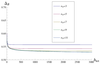
In figure 4 we have plotted the bound for various values of the order of the differential operator. As expected, is monotonically decreasing in . We find that converges very quickly in for small Hodge numbers. The weakest bound is for vanishing Hodge numbers, for which we find . Note in particular that this means that the lowest lying state is always a non-BPS state.
4.5 Large Hodge numbers
We can see from figure 4 that for fixed the bound becomes slightly stronger with increasing total Hodge number. Increasing improves the bound, the effect being stronger for larger Hodge numbers. Let us investigate the bound for very large Hodge numbers a bit more carefully. The highest total Hodge number for a Calabi-Yau known to exist at the moment is [36, 37]. In fact, it is still an open question if the number of topologically distinct CY threefolds is finite or not [18, 19]. For this reason it would be very interesting to find a pathology in the spectrum for large enough Hodge numbers, such as the bound becoming negative, hence ruling out unitary sigma-models. In fact, our methods cannot find any such pathology. We show in this section that there is a linear functional bound for asymptotically large . The argument is a variation on that of [15] (correcting the result given there). In the next section, we show that no linear functional bound can be lower than . So the optimal linear functional bound in the limit is , which does not rule out any values of .
To investigate large Hodge numbers it is useful to consider a particular set of linear functionals
| (4.75) |
Instead of Taylor expanding around , we evaluate the matrix element at some arbitrary . This clearly gives a linear functional , which moreover manifestly satisfies the oddness condition. To enforce the semidefinite condition we need to make sure that is nonnegative on the cone . Explicitly this means that for all matrices of the form (4.3) when the are allowed to range over all nonnegative real numbers subject to the unitarity and gap conditions (4.64). Evaluating (4.75) on such an , we have
| (4.76) | |||||
| (4.77) | |||||
so we can estimate
| (4.78) |
In particular this allows us to ignore any multiplicities other than , which is zero for and can take any nonnegative real value for . So satisfies the semidefinite condition if
| (4.79) |
Let us now see what values of we should choose. For , the inequality is clearly not satisfied for large . For , (4.79) is equivalent to
| (4.80) |
Note that is monotonically decreasing in , so we will want to take as large as possible to get the lowest bound on .
The objective we want to maximize is where is given by (4.49),
| (4.81) |
We estimate
| (4.82) |
If there is a value of such that , then modular invariance is impossible and the gap can be excluded´. So we can exclude if
| (4.83) |
Define as the solution to
| (4.84) |
In terms of the Lambert- function,
| (4.85) |
We have semidefinite for and we have for , so we have a bound
| (4.86) |
provided . It turns out that for , so this method does give a bound for relatively large Hodge numbers. On the other hand grows monotonically with , so that in view of (4.80) the bound becomes stronger and stronger for larger Hodge numbers. The Lambert function has an asymptotic expansion for large as
| (4.87) |
so that for we find (correcting the bound given in [15]). Finally, as was shown in [15], it follows from that the number of states below grows linearly in for large enough total Hodge number.

4.6 Best possible linear functional bound
Finally let us show that our version of the linear functional method cannot obtain a bound better than . This is essentially a repetition of the argument in the Virasoro case. We show that, for , there is no matrix of differential operators satisfying both the oddness condition and the semidefinite condition. So the linear functional method with real cannot exclude any .
Suppose there were such a matrix . Write . Since , the semidefinite condition (4.65) is
| (4.88) | |||||
| (4.89) | |||||
| (4.90) |
In particular, for all the matrix elements of ,
| (4.91) |
and there exists such that
| (4.92) |
The gaussian integral identity (C.1) says that
| (4.93) |
for a certain function satisfying
| (4.94) |
It then follows from (4.91) that
| (4.95) |
The oddness condition says that, for any matrix of functions of ,
| (4.96) |
Let us take
| (4.97) |
The oddness condition (4.96) becomes
| (4.98) |
Combined with the semidefinite conditions (4.92) and (4.95), this gives . The gaussian integral identity (4.93) then says that for all , and then that also for all . So , so there is no matrix of differential operators satisfying both the oddness condition and the semidefinite condition, so there is no possibility of a linear functional bound that excludes any .
Together with the results from section 4.5, this shows that at least for asymptotically large Hodge numbers we have a complete description of the linear functional bound.
Acknowledgment
We thank S. Hellerman, A. Konechny, and C. Schmidt-Colinet for useful discussions, and S. El-Showk for helpful discussions of the linear functional method. This work was supported by the Rutgers New High Energy Theory Center and by U.S. Department of Energy Grant No. DE-FG02-12ER41813.
Appendix A The matrix
We calculate here the matrix , defined by (2.40) and (2.42), which gives the map from the differential operator to the polynomial ,
| (A.1) |
where
| (A.2) |
and the map is
| (A.3) |
The matrix elements are given by the generating functional
| (A.4) |
from which we see that is upper triangular with diagonal matrix elements and is therefore invertible.
The inverse matrix, reconstructs the differential operator from the polynomial,
| (A.5) |
It can be calculated recursively. The polynomials
| (A.6) |
are defined by
| (A.7) |
so and, for ,
| (A.8) | ||||
| (A.9) |
so
| (A.10) |
Appendix B Implementation of the SDP
We use the SDP solver SDPA [23]. It maximizes a linear function, the objective, over a set of variables, which are positive semidefinite matrices, subject to a set of linear constraints.
The variables are represented as a single positive semidefinite block diagonal matrix , with prescribed block sizes. In our case, for the Virasoro problem, the variable matrix consists of two blocks
| (B.1) |
corresponding to the matrices in (2.51). The linear functions are given by block matrices with the same block structure as the variable matrix , acting by
| (B.2) |
The objective
| (B.3) |
is calculated by combining (2.45) and (2.51). The constraints
| (B.4) |
Finally we need a normalization constraint because the optimization problem is invariant under a simple rescaling of the variable matrix (which is a rescaling of our differential operator ). One possible normalization condition is
| (B.5) |
where
| (B.6) |
This is a robust normalization condition — it singles out one point in each ray in the space of variables.
The block matrices are the data that specify the SDP problem. They depend on via (2.51). For a given value of , we construct the SDP data using the symbolic mathematics program Sage [38], which then hands off the SDP data to the extended-precision solver SDPA-GMP for solution. We found that extended precision arithmetic was needed to get reliable results. The SDP solver returns an approximate maximum and the corresponding solution matrix . All this is implemented as a Sage function . We run the Sage root-finder on this function to find the solution of , to some specified accuracy. The Sage root-finder reports a series of better and better approximate solutions. Our bound is the best approximate solution for which .
We can then verify the bound rigourously by working back from the SDPA solution matrix to calculate the odd differential operator . Then, from , we calculate the polynomial to verify the semidefinite condition (by finding all the roots of ), and we calculate the objective to verify its positivity. All the verification calculations are done in extended precision arithmetic with enough precision to make rounding errors completely negligible. When the verification succeeds, we have a specific differential operator satisfying the oddness and semidefinite conditions, for which . We therefore have a rigorous bound .
The implementation of the case is completely analogous. We are optimizing over a matrix of differential operators. Each differential operator maps to a polynomial . Each polynomial is represented by a pair of positive semidefinite matrices. The variable matrix now consists of 8 blocks, . The polynomials are given by
| (B.7) |
where the are obtained from (4.65). The oddness condition (4.61) leads to constraint matrices . The objective matrix comes from (4.73) and the normalization matrix from (4.70). This normalization is strictly speaking not robust — there is a set of rays of measure zero in the variable space where the normalization condition has no solution. In practice, this difficulty does not arise. The program is simpler to execute. For each value of , a Sage program provides the SDP data to the solver, which returns a bound on .
Appendix C Modular transform of characters
In this section, we make two applications of the two-dimensional gaussian integral
| (C.1) |
C.1 Non-existence of semidefinite linear functionals for
We rewrite (C.1), setting and , to get
| (C.2) |
which is a Fourier transform formula for the modular transformation
| (C.3) |
of the reduced characters defined (as functions of real ) by (2.32),
| (C.4) |
Suppose and suppose is a nonzero linear functional on the real analytic functions of satisfying the oddness condition and also the semidefinite condition
| (C.5) |
From the oddness of and equation (C.3) we get
| (C.6) |
The exponential in (C.6) is strictly positive for any in the range , so (C.6) can only be consistent with (C.5) if for all , which by (C.6) implies for all . So . No such linear functional exists.
C.2 Oddness condition on
The map (2.40) from differential operators to polynomials is
| (C.7) |
Under the modular transform , goes to
| (C.8) |
The oddness condition on is the condition on ,
| (C.9) |
Equation (C.1) gives the identity
| (C.10) |
We interpret the exponential in the integral in terms of the heat kernel for the two dimensional laplacian,
| (C.11) |
| (C.12) |
Leting be the radially symmetric function
| (C.13) |
equation (C.10) becomes
| (C.14) |
Given the radial symmetry of , we can replace with its radial part, and change variable from the radius to , giving
| (C.15) |
where the radial part of is the operator
| (C.16) |
Equation (C.14) is now
| (C.17) |
or
| (C.18) |
where is the reflection in , acting on functions of ,
| (C.19) |
The oddness condition on , equation (C.9), is , or
| (C.20) |
If we separate into its even and odd parts under the reflection ,
| (C.21) |
the oddness condition (C.20) on becomes
| (C.22) |
or
| (C.23) |
Appendix D Representations of the extended SCA
A worldsheet theory for Calabi-Yau compactification of type II superstring theory without flux or for compactification of heterotic string theory has superconformal symmetry. In addition the theory is invariant under spectral flow. Spectral flow by one unit maps the Neveu-Schwarz (NS) sector to itself, taking the symmetry algebra to a set of additional operators that extend the symmetry algebra. This is equivalent to the geometric fact that a CY -fold always carries a holomorphic form. The Hilbert space decomposes into irreducible representations of the extended superconformal algebra. The representation theory of the extended superconformal algebra has been studied in [31, 32, 33], whose main results we repeat here, especially [33], equations (3.2), (3.3), (4.8), (4.9), and (4.11).
For a Calabi-Yau -fold the extended superconformal algebra has central charge . Let us define . The irreducible representations are characterized by the eigenvalues of the generators and acting on the lowest weight subspace of the representation. The character of a representation is
| (D.1) |
Define
| (D.2) |
which is the character of the unextended algebra without any relations (i.e. the character of the , Verma module).
Define the functions
| (D.3) |
In this notation,
| (D.4) |
Massive representations
There are massive representations for each , subject to the unitarity condition . can take one of integer values:
| (D.5) |
The massive characters are
| (D.6) | |||||
| (D.7) |
Note that
| (D.8) |
Massless representations
There are massless representations, all at the unitarity bound . can take one of integer values:
| (D.9) |
The massless characters for are
| (D.10) |
For , the massless characters are given by
| (D.11) |
For , the massless character is
| (D.12) |
Note that, in equation (D.10), substituting , , gives the identity
| (D.13) |
so, for , the massless character is , so we could label the massless representations by with characters given by equation (D.10). Note, however, that loses its meaning if we do this.
When the massive representations reach the unitarity bound , they become reducible and decompose into massless representations as
| (D.14) |
The Witten index of the massive representations is zero. The index of the massless representations is (after spectral flow to the R sector)
| (D.15) |
References
- [1] A. M. Polyakov, Conformal symmetry of critical fluctuations, JETP Lett. 12, 381 (1970) [Pisma Zh. Eksp. Teor. Fiz. 12, 538 (1970)].
- [2] A. A. Migdal, Conformal invariance and bootstrap, Phys. Lett. B 37, 386 (1971).
- [3] A. M. Polyakov, Nonhamiltonian approach to conformal quantum field theory, Zh. Eksp. Teor. Fiz. 66, 23 (1974).
- [4] A. A. Belavin, A. M. Polyakov and A. B. Zamolodchikov, Infinite Conformal Symmetry in Two-Dimensional Quantum Field Theory, Nucl. Phys. B 241, 333 (1984).
- [5] P. Di Francesco, P. Mathieu and D. Senechal, Conformal field theory, New York, USA: Springer (1997)
- [6] R. Rattazzi, V. S. Rychkov, E. Tonni and A. Vichi, Bounding scalar operator dimensions in 4D CFT, JHEP 0812, 031 (2008) [arXiv:0807.0004 [hep-th]].
- [7] F. A. Dolan and H. Osborn, Conformal four point functions and the operator product expansion, Nucl. Phys. B 599, 459 (2001) [hep-th/0011040].
- [8] F. A. Dolan and H. Osborn, Conformal partial waves and the operator product expansion, Nucl. Phys. B 678, 491 (2004) [hep-th/0309180].
- [9] J. A. Shapiro, Loop graph in the dual tube model, Phys. Rev. D 5, 1945 (1972).
- [10] J. L. Cardy, Operator Content of Two-Dimensional Conformally Invariant Theories, Nucl. Phys. B 270, 186 (1986).
- [11] G. W. Moore and N. Seiberg, Classical and Quantum Conformal Field Theory, Commun. Math. Phys. 123, 177 (1989).
- [12] S. Hellerman, A Universal Inequality for CFT and Quantum Gravity, JHEP 1108, 130 (2011). [arXiv:0902.2790 [hep-th]].
- [13] S. Hellerman and C. Schmidt-Colinet, Bounds for State Degeneracies in 2D Conformal Field Theory, JHEP 1108, 127 (2011) [arXiv:1007.0756 [hep-th]].
- [14] D. Friedan, A. Konechny and C. Schmidt-Colinet, Lower bound on the entropy of boundaries and junctions in 1+1d quantum critical systems, Phys. Rev. Lett. 109, 140401 (2012) [arXiv:1206.5395 [hep-th]].
- [15] C. A. Keller and H. Ooguri, Modular Constraints on Calabi-Yau Compactifications, arXiv:1209.4649 [hep-th].
- [16] D. Friedan, A. Konechny and C. Schmidt-Colinet, Precise lower bound on Monster brane boundary entropy, JHEP 1307, 099 (2013) [arXiv:1305.2122 [hep-th]].
- [17] S. El-Showk and M. F. Paulos, Bootstrapping Conformal Field Theories with the Extremal Functional Method, arXiv:1211.2810 [hep-th].
- [18] S.-T. Yau, Review of Geometry and Analysis, Asian J. Math 4, 235 (2000).
- [19] M. Reid, The moduli space of 3-folds with K = 0 may nevertheless be irreducible, Math. Ann. 278, 329 (1987).
- [20] B. D. Craven and J. J. Kohila, Generalizations of Farkas theorem, SIAM Journal on Mathematical Analysis Vol. 8, No. 6 (1977).
- [21] D. Poland, D. Simmons-Duffin and A. Vichi, Carving Out the Space of 4D CFTs, JHEP 1205, 110 (2012) [arXiv:1109.5176 [hep-th]].
- [22] G. Pólya and G. Szegö, Problems and Theorems in Analysis, Vol. II, p. 78, Springer Verlag, New York-Heidelberg-Berlin, 2004.
- [23] M. Yamashita, K. Fujisawa, M. Fukuda, K. Nakata and M. Nakata, A high-performance software package for semidefinite programs: SDPA 7, Research Report B-463, Dept. of Mathematical and Computing Science, Tokyo Institute of Technology, Tokyo, Japan, September, 2010. SDPA web page, http://sdpa.sourceforge.net/.
- [24] M. Ademollo, et al., Supersymmetric strings and color confinement, Phys. Lett. B 62, 105 (1976).
- [25] M. Ademollo, et al., Dual string with U(1) color symmetry, Nucl. Phys. B 111, 77 (1976).
- [26] W. Boucher, D. Friedan and A. Kent, Determinant formulae and unitarity for the N=2 superconformal algebras in two-dimensions or exact results on string compactification, Phys. Lett. B 172, 316 (1986).
- [27] V. K. Dobrev, Characters Of The Unitarizable Highest Weight Modules Over The N=2 Superconformal Algebras, Phys. Lett. B 186, 43 (1987).
- [28] E. Kiritsis, Character formulae and the structure of the representations of the N=1, N=2 superconformal algebras, Int. J. Mod. Phys. A 3, 1871 (1988).
- [29] T. Kawai, Y. Yamada and S. -K. Yang, Elliptic genera and N=2 superconformal field theory, Nucl. Phys. B 414, 191 (1994) [hep-th/9306096].
- [30] A. Schwimmer and N. Seiberg, Comments on the N=2, N=3, N=4 Superconformal Algebras in Two-Dimensions, Phys. Lett. B 184, 191 (1987).
- [31] S. Odake, Extension of N=2 Superconformal Algebra and Calabi-Yau Compactification, Mod. Phys. Lett. A 4, 557 (1989).
- [32] S. Odake, Character Formulas of an Extended Superconformal Algebra Relevant to String Compactification, Int. J. Mod. Phys. A 5, 897 (1990).
- [33] S. Odake, c = 3-d conformal algebra with extended supersymmetry, Mod. Phys. Lett. A 5, 561 (1990).
- [34] M. Eichler and D. Zagier, The Theory of Jacobi Forms, Birkhäuser, 1985.
- [35] V. Gritsenko, Elliptic Genus of Calabi-Yau Manifolds and Jacobi and Siegel Modular Forms, Algebra i Analiz, 11:5 (1999), 100Ð125 [math.AG/9906190].
- [36] M. Kreuzer and H. Skarke, Complete classification of reflexive polyhedra in four-dimensions, Adv. Theor. Math. Phys. 4, 1209 (2002) [hep-th/0002240].
- [37] W. Taylor, On the Hodge structure of elliptically fibered Calabi-Yau threefolds, JHEP 1208, 032 (2012) [arXiv:1205.0952 [hep-th]].
- [38] William A. Stein, et al., Sage Mathematics Software (Version 5.9), The Sage Development Team, 2013, http://www.sagemath.org.