When is the majority-vote classifier beneficial?

In his seminal paper, Schapire (1990) proved that weak learning algorithms — ones that perform only slightly better than random guessing — can be turned into ones capable of achieving arbitrarily high accuracy. Does our conclusion stand in the face of Schapire’s result? Certainly not. Schapire’s constructive proof shows how one can sequentially boost weak learners into strong ones (Freund and Schapire 1996, see also), but his proof certainly does not imply that one can always do so with a simple majority-vote mechanism — a common misconception.

Such widespread misconceptions are perhaps fueled partially by incomplete understandings of Breiman’s influential algorithms — namely, bagging (Breiman 1996) and random forest (Breiman 2001) — that do indeed use the majority-vote mechanism, and partially by the popular lessons drawn from the highly-publicized million-dollar Netflix contest (Van Buskirk 2009, see, e.g.,) that testify to the wisdom of crowds (Surowiecki 2004). But it is a logic flaw to conclude that the majority-vote mechanism can be used to improve any collection of weak learners simply because it has had a number of successful applications. Even for Surowiecki (2004), crowd wisdom is not always the result of simple majority voting. An important goal that we hope to accomplish with our analysis is to put a halt to the spread of such common misconceptions.

We will write

	$\displaystyle\mu_{p}\equiv\mbox{E}_{p}(g_{n})\equiv\mbox{E}(g_{n}|y=1),$		$\displaystyle\mbox{Var}_{p}(g_{n})\equiv\mbox{Var}(g_{n}|y=1),$
	$\displaystyle\mu_{q}\equiv\mbox{E}_{q}(g_{n})\equiv\mbox{E}(g_{n}|y=0),$		$\displaystyle\mbox{Var}_{q}(g_{n})\equiv\mbox{Var}(g_{n}|y=0).$

Let

$\displaystyle\sigma_{p}^{2}\equiv\lim_{n\rightarrow\infty}\left[\frac{\mbox{Var}_{p}(g_{n})}{n}\right]\quad\mbox{and}\quad\sigma_{q}^{2}\equiv\lim_{n\rightarrow\infty}\left[\frac{\mbox{Var}_{q}(g_{n})}{n}\right].$

(6)

Our argument is asymptotic for $n\rightarrow\infty$. That is to say, we assume that we have access to a fairly large collection of classifiers. This is certainly the case for both bagging (Breiman 1996) and random forest (Breiman 2001). Our strategy is very simple. The error rate of the individual classifier $f_{i}$ is given by

	$\displaystyle\mbox{err}_{i}$	$\displaystyle\equiv$	$\displaystyle\mbox{Pr}(f(\mathbf{x};\theta_{i})=0|y=1)\mbox{Pr}(y=1)+\mbox{Pr}(f(\mathbf{x};\theta_{i})=1|y=0)\mbox{Pr}(y=0)$
		$\displaystyle=$	$\displaystyle(1-p_{i})\pi+q_{i}(1-\pi).$

Thus, the mean individual error of classifiers in the collection $\mathcal{F}_{n}$ is

$\displaystyle\mbox{err}\equiv\mbox{E}_{\mathcal{P}_{\theta}}(\mbox{err}_{i})=\mbox{E}_{\mathcal{P}_{\theta}}\left[(1-p_{i})\pi+q_{i}(1-\pi)\right]=(1-p)\pi+q(1-\pi),$

(7)

whereas the error rate of the majority-vote classifier, $g_{n}$, is simply

$\displaystyle\mbox{Err}(n)$

$\displaystyle\equiv$

$\displaystyle\mbox{Pr}\left(g_{n}\leq n/2\big|y=1\right)\mbox{Pr}(y=1)+\mbox{Pr}\left(g_{n}>n/2\big|y=0\right)\mbox{Pr}(y=0).$

First, we apply the central limit theorem (some technical details in Section 2.2) and estimate $\mbox{Err}(n)$ by

$\displaystyle\widehat{\mbox{Err}}(n)=\left[\Phi\left(\frac{n/2-\mu_{p}}{\sigma_{p}\sqrt{n}}\right)\right]\pi+\left[1-\Phi\left(\frac{n/2-\mu_{q}}{\sigma_{q}\sqrt{n}}\right)\right](1-\pi),$

(8)

where $\Phi(\cdot)$ is the cumulative distribution function of the standard $\mbox{N}(0,1)$ random variable. Then, we compare $\widehat{\mbox{Err}}(n)$ with the mean individual error, given in (7). The difference,

$$\Delta(n)\equiv\widehat{\mbox{Err}}(n)-\mbox{err},$$

is one way to measure whether $g_{n}$ provides any genuine benefit over a typical $f_{i}$, with $\Delta(n)<0$ being an indication of true benefit. We pay particular attention to the limiting quantity,

$$\Delta(\infty)\equiv\lim_{n\rightarrow\infty}\Delta(n),$$

which turns out to have interesting phase transitions in the space of $(p,q)$; see Section 2.3 below.

In order to apply the central limit theorem so as to estimate $\mbox{Err}(n)$ by (8), the key technical requirement is that both limits $\sigma_{p}$ and $\sigma_{q}$ are finite and non-zero (Billingsley 1995; Bradley 2005, see, e.g.,).

Using the result of Theorem 1 and Table 1 in particular, we can compute easily — for any given position $(p,q)$ in the open unit square — the value of

$$\Delta(\infty)=\lim_{n\rightarrow\infty}\widehat{\mbox{Err}}(n)-\mbox{err},$$

and determine whether $\Delta(\infty)$ is positive, negative, or zero. The proof of Theorem 1 given below (Section 2.2.1) explains the origin of the phase-transition phenomenon, but readers not interested in the details may skip it and jump right to Section 2.3.

Table 2 shows the values of $\Delta(\infty)$ as they vary in the space of $(p,q)$. Notice the abrupt phase transitions occurring at the boundaries, $p=1/2$ and $q=1/2$. In particular, for fixed $q$, there is a jump of size $\pi/2$ going from $p<1/2$, $p=1/2$, to $p>1/2$; for fixed $p$, there is a jump of size $1/2-\pi/2$ going from $q<1/2$, $q=1/2$, to $q>1/2$.

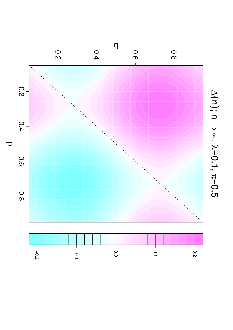
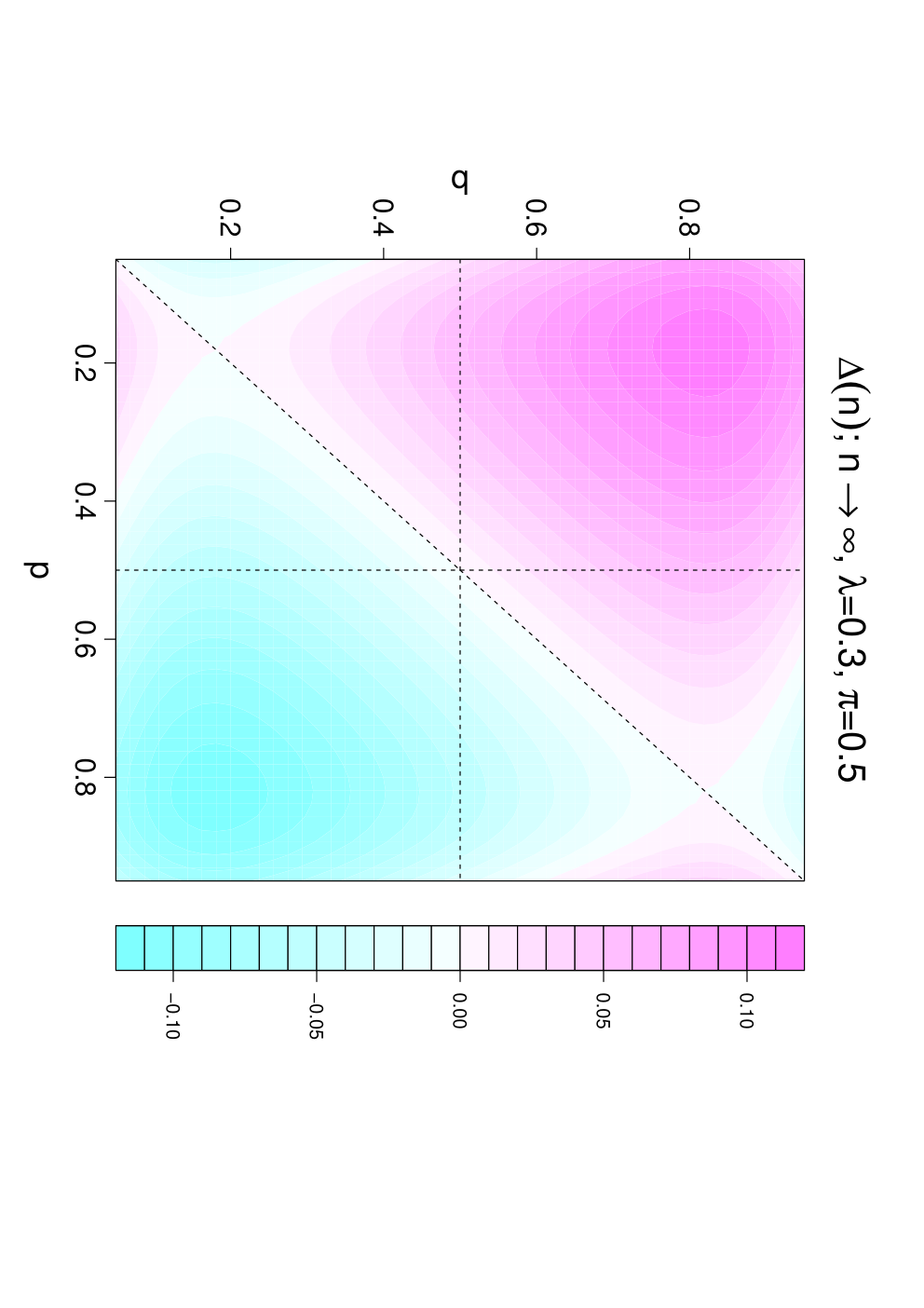
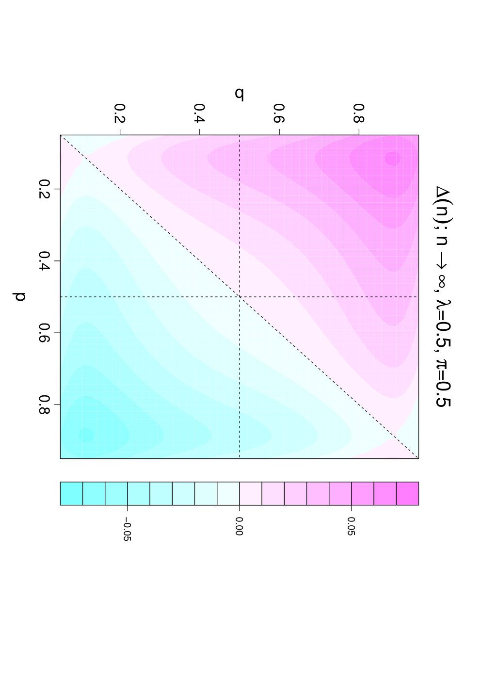
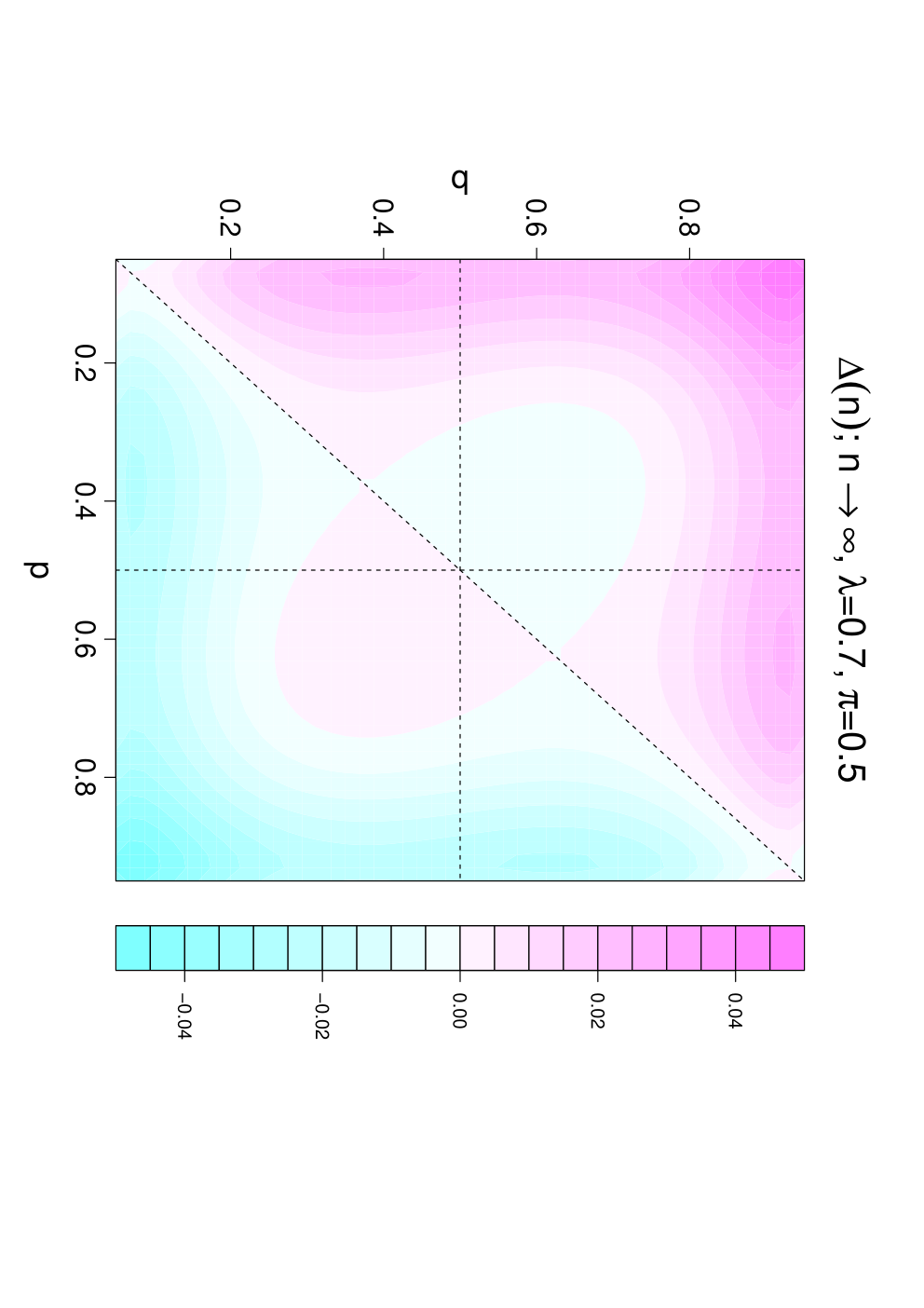
Figure 2 shows $\Delta(n)$ as a function of $(p,q)$ for $\pi=0.25,0.5$ and $0.75$ while fixing $n=1000$. It is evident from both Figure 2 and Table 2 that $\pi\in(0,1)$ merely changes the shape of the function $\Delta(\infty)$ within each region — as specified by whether each of $p,q$ is larger than, equal to, or smaller than $1/2$ — and the size of the jumps between these regions, but it does not cause these phase transitions to appear or to disappear. In other words, the phase transition phenomenon at $p=1/2$ and at $q=1/2$ is universal regardless of what value $\pi$ takes on.

While a phase diagram can be produced easily for any value of $\pi$, for the remainder of the paper we shall focus on $\pi=1/2$, a case that deserves special attention for binary classification (Table 3).

Recall from (4)-(5) that $p$ and $q$ are the average TPR and the average FPR of the collection $\mathcal{F}_{n}$. Intuitively, it is natural for us to require that, on average, individual classifiers in $\mathcal{F}_{n}$ should be more likely to predict $\hat{y}=1$ when $y=1$ than when $y=0$, that is, we would like to have

$$p>q.$$

Indeed, when $\pi=1/2$, we easily can see that the mean individual error is smaller than the error of random guessing if and only if $p>q$:

$$\mbox{err}=(1-p)\pi+q(1-\pi)=\frac{1-(p-q)}{2}<\frac{1}{2}\quad\Leftrightarrow\quad p>q.$$

Therefore, based on “conventional wisdom” (Section 1.1), one may be tempted to think that, on average, $\mathcal{F}_{n}$ can be considered a collection of weak classifiers so long as $p>q$, and that taking majority votes over such a collection should be beneficial. But, according to our preceding analysis, the condition $p>q$ alone is actually “too weak” and not enough by itself to ensure that $g_{n}$ is truly beneficial.

Figure 3 contains the corresponding phase diagram showing the sign of $\Delta(\infty)$ for the case of $\pi=1/2$. The phase diagram clearly shows that we need more than $p>q$ in order to have $\Delta(\infty)\leq 0$. More specifically, we see that we need $p$ and $q$ to be on different sides of $1/2$, that is,

$$p\geq 1/2\geq q.$$

The condition $p>q$ by itself is too weak. If, for example,

$$p>q>1/2\quad\mbox{or}\quad 1/2>p>q,$$

then the majority-vote classifier $g_{n}$ actually performs worse! In other words, even if $p>q$ so that a typical classifier in $\mathcal{F}_{n}$ can be considered a weak learner, the majority-vote mechanism only makes matters worse if $p$ and $q$ are on the same side of $1/2$.

This is because, if $p$ and $q$ are on the same side of $1/2$, then, as we take majority votes over more and more weak learners, $g_{n}$ will eventually classify everything into the same class with probability one (and become useless as a result). In particular, $g_{n}$ will classify everything into class 1 if both $p$ and $q$ are greater than $1/2$, and into class 0 if both are less than $1/2$.

Perhaps somewhat curiously, symmetry leads to the conclusion that it is possible to have $\Delta(\infty)<0$ even when $p<q$, e.g., if $1/2<p<q$ or $p<q<1/2$ — again, see Figure 3. However, this is not so much because $g_{n}$ is a good classifier, but because the collection $\mathcal{F}_{n}$ is very poor when $p<q$; in fact, a typical classifier from $\mathcal{F}_{n}$ is worse than random, and more likely to predict $\hat{y}=1$ when $y=0$ and vice versa. But, as we’ve pointed out earlier, if $p$ and $q$ are on the same side of $1/2$, $g_{n}$ will eventually classify everything into the same class. Now, that’s useless indeed, but it surely is still better than classifying things into the opposite class! Though conceptually curious, these cases are not of practical interest.

What does all this mean? Given a collection of classifiers, $\mathcal{F}_{n}$, intuitively one may be tempted to think of it as a collection of weak learners if its average TPR is greater than its average FPR (i.e., if $p>q$), but taking majority votes over such a collection cannot be guaranteed to produce improved results. To obtain improvements (assuming equal priors), the collection must have an average TPR of at least $50\%$ (i.e., $p\geq 0.5$) and an average FPR of at most $50\%$ (i.e., $q\leq 0.5$). In other words, the typical classifier in the collection cannot be arbitrarily weak.

By the law of total variance, we have

	$\displaystyle\mbox{Var}_{p}(f_{i})$	$\displaystyle\equiv$	$\displaystyle\mbox{Var}(f_{i}|y=1)$
		$\displaystyle=$	$\displaystyle\mbox{E}_{\mathcal{P}_{\theta}}\left[\mbox{Var}(f_{i}|\theta_{i};y=1)\right]+\mbox{Var}_{\mathcal{P}_{\theta}}\left[\mbox{E}(f_{i}|\theta_{i};y=1)\right]$
		$\displaystyle=$	$\displaystyle\mbox{E}_{\mathcal{P}_{\theta}}\left[p_{i}(1-p_{i})\right]+\mbox{Var}_{\mathcal{P}_{\theta}}\left[p_{i}\right]$
		$\displaystyle=$	$\displaystyle\mbox{E}_{\mathcal{P}_{\theta}}(p_{i})-\mbox{E}_{\mathcal{P}_{\theta}}(p_{i}^{2})+\mbox{Var}_{\mathcal{P}_{\theta}}\left(p_{i}\right)$
		$\displaystyle=$	$\displaystyle\mbox{E}_{\mathcal{P}_{\theta}}(p_{i})-\left[\mbox{E}^{2}_{\mathcal{P}_{\theta}}(p_{i})+\mbox{Var}_{\mathcal{P}_{\theta}}(p_{i})\right]+\mbox{Var}_{\mathcal{P}_{\theta}}\left(p_{i}\right)$
		$\displaystyle=$	$\displaystyle p(1-p).$

While it is obvious that $\mbox{Var}(f_{i}|\theta_{i};y=1)=p_{i}(1-p_{i})$, it is perhaps not so obvious that, under $\theta_{i}\overset{iid}{\sim}\mathcal{P}_{\theta}$, we simply have $\mbox{Var}(f_{i}|y=1)=p(1-p)$ as well. The same argument establishes that $\mbox{Var}_{q}(f_{i})=q(1-q)$. Furthermore, following the definitions of $\mbox{Var}_{p}(f_{i})$ and $\mbox{Var}_{q}(f_{i})$, we define

$$\mbox{Cov}_{p}(f_{i},f_{j})=\mbox{Cov}(f_{i},f_{j}|y=1),\qquad\mbox{Cov}_{q}(f_{i},f_{j})=\mbox{Cov}(f_{i},f_{j}|y=0),$$

as well as

$$\mbox{Corr}_{u}(f_{i},f_{j})=\frac{\mbox{Cov}_{u}(f_{i},f_{j})}{\sqrt{\mbox{Var}_{u}(f_{i})\mbox{Var}_{u}(f_{j})}}$$

for $u=p,q$.

Suppose that $\mbox{Corr}_{u}(f_{i},f_{j})=0$ for all $i\neq j$ and $u=p,q$ — e.g., if $f_{1},f_{2},...,f_{n}$ are conditionally independent given either $y=0$ or $y=1$, then

$\displaystyle\sigma_{p}^{2}=\lim_{n\rightarrow\infty}\left[\frac{\mbox{Var}_{p}(g_{n})}{n}\right]=\lim_{n\rightarrow\infty}\left[\frac{np(1-p)}{n}\right]=p(1-p)\in(0,\infty).$

Similarly, we can conclude that $0<\sigma_{q}^{2}<\infty$ as well, so the condition of Theorem 1 is satisfied. In reality, however, the conditional independence assumption is not very realistic. Since the individual classifiers $f_{1},f_{2},...,f_{n}$ typically rely on the same training data $\{(y_{i},\mathbf{x}_{i})\}_{i=1}^{N}$ to “go after” the same quantity of interest, namely $\mbox{Pr}(y|\mathbf{x})$, there is usually an non-ignorable amount of correlation among them.

Alternatively, suppose that, for all $i,j$ and $u=p,q$, $\mbox{Corr}_{u}(f_{i},f_{j})=\gamma^{|i-j|}$ for some $0<\gamma<1$. The correct interpretation of this assumption is as follows: between a given classifier $f_{i}$ and other members of $\mathcal{F}_{n}$, the largest correlation is $\gamma$; the second largest correlation is $\gamma^{2}$; and so on. The exponential decay structure is admittedly artificial, but such a structure will ensure that both limits $\sigma_{p}$ and $\sigma_{q}$ are, again, finite and non-zero. In particular,

	$\displaystyle\mbox{Var}_{p}(g_{n})$	$\displaystyle=$	$\displaystyle\sum_{i=1}^{n}\mbox{Var}_{p}(f_{i})+\sum_{i\neq j}\mbox{Cov}_{p}(f_{i},f_{j})$		(11)
		$\displaystyle=$	$\displaystyle np(1-p)+2\left[(n-1)\gamma+(n-2)\gamma^{2}+...+\gamma^{n-1}\right]p(1-p)$
		$\displaystyle=$	$\displaystyle np(1-p)\left[1+2\sum_{j=1}^{n-1}\left(1-\frac{j}{n}\right)\gamma^{j}\right],$

which means

$\displaystyle\sigma_{p}^{2}=\lim_{n\rightarrow\infty}\left[\frac{\mbox{Var}_{p}(g_{n})}{n}\right]=p(1-p)\left[1+2\sum_{j=1}^{\infty}\gamma^{j}\right]=p(1-p)\left[\frac{1+\gamma}{1-\gamma}\right]\in(0,\infty)$

(12)

and likewise for $\sigma_{q}^{2}$. The limit going from (11) to (12) as $n\rightarrow\infty$ is standard and frequently mentioned in the Markov chain Monte Carlo (MCMC) literature (e.g., Liu 2001, Section 5.8).

Figure 4 shows the behaviors of $\widehat{\mbox{Err}}(n)$ and $\Delta(n)$ for $\pi=1/2$, $n=100$, and $\gamma=0$ (uncorrelated case; Section 3.2), $\gamma=0.4$, $\gamma=0.8$. We can see that the maximal amount of improvement obtainable by $g_{n}$ over a typical $f_{i}$ is about $40$ percentage points when $\gamma=0$, but only a little over $20$ percentage points when $\gamma=0.8$. In other words, when the classifiers are correlated, more of them are needed in order for $g_{n}$ to achieve the same level of performance — hardly a surprising conclusion. Moreover, for the same $n=100$, both $\widehat{\mbox{Err}}(n)$ and $\Delta(n)$ are clearly closer to their asymptotic limits (see Section 2) when $\gamma=0$. Overall, the effect of $\gamma>0$ is to slow down the convergence, although the same limits as in the (unrealistic) independent/uncorrelated case ($\gamma=0$) are eventually achieved.

Compared with the conditional independent case of Section 3.2, the scenario considered in this section is slightly more realistic. The essence of the correlation model $\gamma^{|i-j|}$, of course, is that most of the correlations are kept quite small so the technical condition of Theorem 1 can still be satisfied.

For collections generated by an i.i.d. mechanism such as (3), it is perhaps even more realistic to consider the case that $\mbox{Corr}_{u}(f_{i},f_{j})=\lambda\in(0,1)$ for all $i\neq j$ and $u=p,q$. But then, we have

	$\displaystyle\mbox{Var}_{p}(g_{n})$	$\displaystyle=$	$\displaystyle\sum_{i=1}^{n}\mbox{Var}_{p}(f_{i})+\sum_{i\neq j}\mbox{Cov}_{p}(f_{i},f_{j})$		(13)
		$\displaystyle=$	$\displaystyle np(1-p)+\lambda\times n(n-1)p(1-p)$
		$\displaystyle=$	$\displaystyle n^{2}\lambda p(1-p)+n(1-\lambda)p(1-p).$

This means

$\displaystyle\sigma_{p}^{2}=\lim_{n\rightarrow\infty}\left[\frac{\mbox{Var}_{p}(g_{n})}{n}\right]=p(1-p)\lim_{n\rightarrow\infty}[n\lambda+(1-\lambda)]=\infty,$

and likewise for $\sigma_{q}^{2}$. That is, the condition of Theorem 1 no longer holds.

Based on the three cases discussed above, it becomes fairly clear that the key technical condition of Theorem 1 — namely, $\sigma_{p},\sigma_{q}<\infty$ — is merely an indirect way to control the total amount of correlation among the individual classifiers in $\mathcal{F}_{n}$. In his “random forest” paper, Breiman (2001) proved that, all other things being equal, classifiers having lower correlations with one another would form a better forest. Our analysis suggests that, even under fairly ideal conditions (well-controlled amount of total correlation), the majority-vote mechanism still requires more than $p>q$ in order to be truly beneficial.

To get a sense of what could happen if the total amount of correlation should go “out of control”, let us go back to Case 3 and ask a bold question: what if we went ahead and abused the central limit theorem in this case, even though the usual requirement (9) is not met? Since $\sigma_{p},\sigma_{q}=\infty$, we replace $(\sigma_{p}\sqrt{n},\sigma_{q}\sqrt{n})$ with $([\mbox{Var}_{p}(g_{n})]^{1/2},[\mbox{Var}_{q}(g_{n})]^{1/2})$ in (8). For large $n$, (13) implies that

$\displaystyle[\mbox{Var}_{p}(g_{n})]^{1/2}\approx n\sqrt{\lambda p(1-p)}\quad\mbox{and}\quad[\mbox{Var}_{q}(g_{n})]^{1/2}\approx n\sqrt{\lambda q(1-q)},$

(14)

so our (abusive) estimate of $\mbox{Err}(n)$ as $n\rightarrow\infty$ becomes

$\displaystyle\widehat{\mbox{Err}}(\infty)=\left[\Phi\left(\frac{1/2-p}{\sqrt{\lambda p(1-p)}}\right)\right]\pi+\left[1-\Phi\left(\frac{1/2-q}{\sqrt{\lambda q(1-q)}}\right)\right](1-\pi).$

(15)

This is equivalent to the independent case (Section 3.2) with $n=1/\lambda$. That is, a large collection (of classifiers) with conditional pairwise correlation equal to $\lambda$ will behave essentially like a conditionally independent (or uncorrelated) collection of size $1/\lambda$. Despite having abused the central limit theorem, this conclusion does not appear to be totally unreasonable after all.

Figure 5 shows the behavior of $\Delta(\infty)$ for $\pi=1/2$ and $\lambda=0.1,0.3,0.5,0.7$, having replaced $(\sigma_{p}\sqrt{n},\sigma_{q}\sqrt{n})$ in (8) with $([\mbox{Var}_{p}(g_{n})]^{1/2},[\mbox{Var}_{q}(g_{n})]^{1/2})$ as given in (14). Since the case of $\lambda=0.1$ (relatively low correlation) is “like” having an independent collection of size $1/\lambda=10$, the behavior of $\Delta(\infty)$ is still close enough to what our theory has predicted. For the case of $\lambda=0.7$ (very high correlation), however, even the “golden region” predicted by our theory — namely $p\geq 1/2\geq q$ — fails to guarantee that $g_{n}$ is useful. The majority-vote mechanism cannot reduce the error rate unless the average FPR is very low or the average TPR is very high — the south-east region shaped like a mirror image of the letter “L”. Even then, the maximal amount of improvement obtainable is only a little over $4$ percentage points.

References

- Billingsley (1995) Billingsley, P. (1995). Probability and Measure. Wiley, New York, 3rd edition.
- Bradley (2005) Bradley, R. (2005). Basic properties of strong mixing conditions: A survey and some open questions. Probability Surveys, 2, 107–144.
- Breiman (1996) Breiman, L. (1996). Bagging predictors. Machine Learning, 24(2), 123–140.
- Breiman (2001) Breiman, L. (2001). Random forests. Machine Learning, 45(1), 5–32.
- Egan (1975) Egan, J. P. (1975). Signal Detection Theory and ROC Analysis. Academic Press, New York.
- Freund and Schapire (1996) Freund, Y. and Schapire, R. (1996). Experiments with a new boosting algorithm. In Proceedings of the 13th International Conference on Machine Learning, pages 148–156. Morgan Kaufmann, San Francisco, CA, USA.
- Green and Swets (1966) Green, D. M. and Swets, J. A. (1966). Signal Detection Theory and Psychophysics. Wiley, New York.
- Ho (1998) Ho, T. K. (1998). The random subspace method for constructing decision forests. IEEE Transactions on Pattern Analysis and Machine Intelligence, 20(8), 832–844.
- Kearns and Valiant (1989) Kearns, M. and Valiant, L. G. (1989). Cryptographic limitations on learning Boolean formulae and finite automata. In Proceedings of the 21st Annual ACM Symposium on Theory of Computing, pages 433–444.
- Kuncheva (2004) Kuncheva, L. I. (2004). Combining Pattern Classifiers: Method and Algorithms. Wiley, New York.
- Liu (2001) Liu, J. S. (2001). Monte Carlo Strategies in Scientific Computing. Springer-Verlag, New York.
- Narasimhamurthy (2005) Narasimhamurthy, A. (2005). Theoretical bounds of majority voting performance for a binary classification problem. IEEE Transactions on Pattern Analysis and Machine Intelligence, 27(12), 1988–1995.
- Pepe (2003) Pepe, M. S. (2003). The Statistical Evaluation of Medical Tests for Classification and Prediction. Oxford University Press, New York.
- Schapire (1990) Schapire, R. (1990). The strength of weak learnability. Machine Learning, 5, 197–227.
- Surowiecki (2004) Surowiecki, J. (2004). The Wisdom of Crowds. Doubleday, New York.
- Swets (1988) Swets, J. A. (1988). Measuring the accuracy of diagnostic systems. Science, 240, 1285–1293.
- Swets and Pickett (1982) Swets, J. A. and Pickett, R. M. (1982). Evaluation of Diagnostic Systems: Methods from Signal Detection Theory. Academic Press, New York.
- Van Buskirk (2009) Van Buskirk, E. (2009). How the Netflix prize was won. Wired magazine online, http://www.wired.com/business/2009/09/how-the-netflix-prize-was-won/.
- Webb (2002) Webb, A. R. (2002). Statistical Pattern Recognition. Wiley, New York, 2nd edition.