Inspiral-merger-ringdown waveforms of spinning, precessing black-hole binaries in the effective-one-body formalism

Throughout the paper, we adopt geometric units $G=c=1$ and the Einstein summation convention, unless otherwise specified. The masses of the BHs are $m_{1}$ and $m_{2}$ and we choose $m_{1}\geq m_{2}$. The total mass, mass ratio and symmetric mass ratio are $M=m_{1}+m_{2}$, $q=m_{1}/m_{2}$ and $\nu=m_{1}m_{2}/M^{2}$, respectively. The position, linear momentum and spin vectors of the BHs are $\mbox{\boldmath${r}$}_{i}(t)$, $\mbox{\boldmath${p}$}_{i}(t)$ and $\mbox{\boldmath${S}$}_{i}(t)=\chi_{i}m_{i}^{2}\hat{\mbox{\boldmath${S}$}}_{i}$, where $i=1$, $2$ and $\chi_{i}$ is the dimensionless spin magnitude. In the EOB framework, we solve the time evolution of the relative (rescaled) position vector $\mbox{\boldmath${r}$}(t)\equiv\left(\mbox{\boldmath${r}$}_{1}(t)-\mbox{\boldmath${r}$}_{2}(t)\right)/M$, the center-of-mass–frame (rescaled) momentum vector $\mbox{\boldmath${p}$}(t)\equiv\mbox{\boldmath${p}$}_{1}(t)/\mu=-\mbox{\boldmath${p}$}_{2}(t)/\mu$, and the spins variables $\mbox{\boldmath${S}$}_{1}(t)$ and $\mbox{\boldmath${S}$}_{2}(t)$.

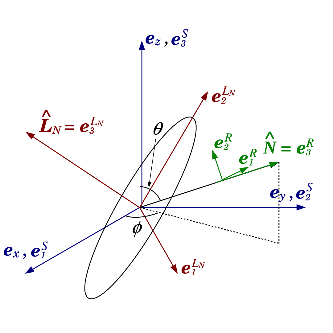
We start with an arbitrary orthonormal basis $\{\mbox{\boldmath${e}$}_{x},\mbox{\boldmath${e}$}_{y},\mbox{\boldmath${e}$}_{z}\}$. Without loss of generality, we align the initial relative position vector $\mbox{\boldmath${r}$}_{0}$ with $\mbox{\boldmath${e}$}_{x}$ and the initial orbital orientation $[\hat{\mbox{\boldmath${L}$}}_{N}]_{0}\equiv\hat{\mbox{\boldmath${L}$}}_{N}(0)\equiv\mbox{\boldmath${r}$}_{0}\times\dot{\mbox{\boldmath${r}$}}_{0}/|\mbox{\boldmath${r}$}_{0}\times\dot{\mbox{\boldmath${r}$}}_{0}|$ with $\mbox{\boldmath${e}$}_{z}$, where we indicate with an over-dot the time derivative and $\dot{\mbox{\boldmath${r}$}}_{0}=\dot{\mbox{\boldmath${r}$}}(0)$ is the initial relative velocity. The initial spin directions are specified by the spherical coordinates $\theta^{S}_{1}$, $\phi^{S}_{1}$, $\theta^{S}_{2}$ and $\phi^{S}_{2}$ associated with this basis.

In the nonprecessing case, $\hat{\mbox{\boldmath${L}$}}_{N}$ is a constant and it is natural to choose a source frame described by the (unit) basis vectors $\{\mbox{\boldmath${e}$}_{1}^{S},\mbox{\boldmath${e}$}_{2}^{S},\mbox{\boldmath${e}$}_{3}^{S}\}$ whose $\mbox{\boldmath${e}$}_{3}^{S}$ is aligned with $\hat{\mbox{\boldmath${L}$}}_{N}$. In the precessing case, we choose to align the source frame $\{\mbox{\boldmath${e}$}_{1}^{S},\mbox{\boldmath${e}$}_{2}^{S},\mbox{\boldmath${e}$}_{3}^{S}\}$ with $\{\mbox{\boldmath${e}$}_{x},\mbox{\boldmath${e}$}_{y},\mbox{\boldmath${e}$}_{z}\}$. The basis vector $\mbox{\boldmath${e}$}_{3}^{S}$ is aligned with the initial orbital orientation $\hat{\mbox{\boldmath${L}$}}_{N}(0)$ but not with $\hat{\mbox{\boldmath${L}$}}_{N}(t)$ at later times.

The GW polarizations $h_{+}$ and $h_{\times}$ can be obtained by projecting the strain tensor $h_{ij}$ onto the radiation frame described by the (unit) basis vectors $\{\mbox{\boldmath${e}$}_{1}^{R},\mbox{\boldmath${e}$}_{2}^{R},\mbox{\boldmath${e}$}_{3}^{R}\equiv\hat{\mbox{\boldmath${N}$}}\}$, the basis vector $\hat{\mbox{\boldmath${N}$}}$ being along the direction of propagation of the wave (see Fig. 1). That is

where the basis vectors $\mbox{\boldmath${e}$}_{1}^{R}$ and $\mbox{\boldmath${e}$}_{2}^{R}$ are defined by (see Fig. 1)

In the source frame $\{\mbox{\boldmath${e}$}_{1}^{S},\mbox{\boldmath${e}$}_{2}^{S},\mbox{\boldmath${e}$}_{3}^{S}\}$, we can decompose the polarizations $h_{+}$ and $h_{\times}$ in $-2$ spin-weighted spherical harmonics ${}_{-2}Y_{\ell m}(\theta,\phi)$ as

The modes $h_{\ell m}$ can be calculated by applying the orthogonality condition valid for the ${}_{-2}Y_{\ell m}(\theta,\phi)$’s. Thus

where $\theta$ and $\phi$ are the inclination and azimuthal angles of the unit vector $\hat{\mbox{\boldmath${N}$}}$ as measured in the source frame. Note that in the above expressions, we omit the dependence of the GW polarizations on time and binary parameters.

In the nonprecessing case, the orbital orientation is constant and coincides with the directions of the orbital angular momentum $\mbox{\boldmath${L}$}\equiv\mu M\mbox{\boldmath${r}$}\times\mbox{\boldmath${p}$}$, the Newtonian angular momentum $\mbox{\boldmath${L}$}_{N}\equiv\mu M\mbox{\boldmath${r}$}\times\dot{\mbox{\boldmath${r}$}}$, and the total angular momentum $\mbox{\boldmath${J}$}\equiv\mbox{\boldmath${L}$}+\mbox{\boldmath${S}$}_{1}+\mbox{\boldmath${S}$}_{2}$. If the source frame is aligned with the orbital orientation, the gravitational polarizations are quite simple and are described mainly by the $(2,2)$ mode and a few subdominant modes [12, 13]. In this case, the wave’s amplitude and frequency increase monotonically during the inspiral and plunge stages, and the amplitudes of the GW modes display a clean hierarchy. By contrast, precessing waveforms decomposed in an inertial source frame show strong amplitude and phase modulations. In this case the amplitudes of the GW modes do not necessarily follow a clean hierarchy [47]. Ideally we would like to conduct comparisons and calibrations between analytical and numerical waveforms in a time dependent source frame that minimizes precession-induced modulations. Fortunately, this is possible if we choose a source frame that precesses with the binary orbital plane [25, 27, 28, 29, 30].

Buonanno, Chen and Vallisneri [25] proposed the precessing convention that neatly disentangles precessional effects from both amplitude and phase evolutions in restricted (i.e., leading-order) PN waveforms. In the precessing convention, the precessing waveform is written as the product of a nonprecessing carrier waveform and a modulation term that collects all precessional effects. In Refs. [25, 27] the authors chose the precessing source frame aligned with the Newtonian orbital angular momentum $\mbox{\boldmath${L}$}_{N}$. In this case, the basis vectors of the precessing source frame, $\{\mbox{\boldmath${e}$}_{1}^{L_{N}}(t),\mbox{\boldmath${e}$}_{2}^{L_{N}}(t),\mbox{\boldmath${e}$}_{3}^{L_{N}}(t)\}$ in Fig. 1, read [25]

where

and $\mbox{\boldmath${\Omega}$}_{L}(t)$ is the angular velocity of the precession of $\hat{\mbox{\boldmath${L}$}}_{N}(t)$ and satisfies $\dot{\hat{\mbox{\boldmath${L}$}}}_{N}(t)=\mbox{\boldmath${\Omega}$}_{L}(t)\times\hat{\mbox{\boldmath${L}$}}_{N}(t)$. Aligning the precessing source frame with $\hat{\mbox{\boldmath${L}$}}_{N}(t)$ in Eq. (5a) removes the precession-induced amplitude modulations. Intuitively, Eqs. (5b)–(6) impose that $\mbox{\boldmath${e}$}_{1}^{L_{N}}(t)$ and $\mbox{\boldmath${e}$}_{2}^{L_{N}}(t)$ follow the precession of $\mbox{\boldmath${e}$}_{3}^{L_{N}}(t)=\hat{\mbox{\boldmath${L}$}}_{N}(t)$, but do not precess around it. The key point of the precessing convention is the removal of all precession-induced modulations from the orbital phase $\Phi(t)$, so that $\Phi(t)$ is simply given by the integral of the (monotonic) orbital frequency $\Omega$, i.e. $\Phi(t)=\int\Omega(t^{\prime})dt^{\prime}$ (see for details Sec. IVA in Ref. [25]). The freedom of choosing the constant of integration, or the initial phase, is degenerate with the only degree of freedom left in defining the precessing source frame, namely a constant rotation of $\mbox{\boldmath${e}$}_{1}^{L_{N}}$ and $\mbox{\boldmath${e}$}_{2}^{L_{N}}$ around $\mbox{\boldmath${e}$}_{3}^{L_{N}}$.

We want to test now the precessing convention on inspiraling PN waveforms computed beyond the restricted approximation, i.e., beyond leading order. We employ the waveforms of Ref. [47] that have spin-amplitude corrections through 1.5PN order. We decompose the $h_{\ell m}$’s in two source frames: (i) the inertial source frame aligned with the initial total angular momentum $\mbox{\boldmath${J}$}_{0}$ [47] and (ii) the precessing source frame $\{\mbox{\boldmath${e}$}_{1}^{L_{N}}(t),\mbox{\boldmath${e}$}_{2}^{L_{N}}(t),\mbox{\boldmath${e}$}_{3}^{L_{N}}(t)\}$ defined by Eqs. (5a)–(6). The waveforms decomposed in the $\mbox{\boldmath${J}$}_{0}$-frame are given explicitly in Appendix B of Ref. [47]. We calculate the waveforms decomposed in the precessing $\mbox{\boldmath${L}$}_{N}(t)$-frame from the waveforms decomposed in the $\mbox{\boldmath${J}$}_{0}$-frame by properly rotating the $h_{\ell m}$ modes.

In general, given a set of spin-weighted spherical harmonics $h_{\ell m}^{(o)}$ decomposed in an original frame and the Euler angles $(\alpha,\beta,\gamma)$ that define the rotation from the original frame to a new frame, the modes $h_{\ell m}^{(n)}$ decomposed in the new frame are given by [47, 48]

where ${D^{\ell\;*}_{m^{\prime}m}}(\alpha,\beta,\gamma)$ is the complex conjugate of the Wigner $D$-matrix

where ${}_{-m^{\prime}}Y_{\ell m}$ is the spherical harmonic of spin-weight $-m^{\prime}$. The transformation is closed among modes with the same index $\ell$. In this paper, we focus on the $\ell=2$ modes both for simplicity and because even when precession is present the $\ell=2$ modes still dominate. Nevertheless, the $\ell>2$ modes are not negligible and we plan to extend the precessing EOB model to those modes in the future, following the same approach we propose and demonstrate here with the $\ell=2$ modes.

In Fig. 2, we compare the $\mbox{\boldmath${J}$}_{0}$-frame and $\mbox{\boldmath${L}$}_{N}(t)$-frame $h_{2m}$ inspiraling waveforms emitted by a BH binary with mass ratio $q=6$ and spin magnitudes $\chi_{1}=\chi_{2}=0.8$. We choose spin orientations that give strong precession-induced modulations. As we can see, there is a clear hierarchy among the $h_{2m}$’s amplitudes when decomposed in the $\mbox{\boldmath${L}$}_{N}(t)$-frame, but not when the decomposition is done in the $\mbox{\boldmath${J}$}_{0}$-frame. In fact, in the $\mbox{\boldmath${J}$}_{0}$-frame, the $(2,1)$ and $(2,0)$ modes have even larger amplitudes than the $(2,2)$ mode. We notice that the strong amplitude and phase modulations of the modes in the $\mbox{\boldmath${J}$}_{0}$-frame almost completely disappear when the $\mbox{\boldmath${L}$}_{N}(t)$-frame is used.

Furthermore, we find it interesting to compare the modes of the precessing waveforms to the ones of a “nonprecessing” binary system having the same mass ratio and $\chi_{i}(t)\equiv\chi_{i}\hat{\mbox{\boldmath${S}$}}_{i}(t)\cdot\hat{\mbox{\boldmath${L}$}}_{N}(t)\,,\;(i=1,2)$. That is to say, we keep only the components of the spin vectors along the direction of the Newtonian angular momentum $\mbox{\boldmath${L}$}_{N}(t)$, and set all the other components to zero. For convenience, we refer to such “nonprecessing” waveforms as the quasi-nonprecessing waveforms. We use the adjective “quasi” because, differently from the nonprecessing waveforms, where the spins are aligned or antialigned with the orbital angular momentum and remain constant throughout the evolution, in the quasi-nonprecessing waveforms the spins evolve (according to Eqs. (11c)–(11d) given below) and over time change their projections onto $\mbox{\boldmath${L}$}_{N}$. As can be seen in Fig. 2, the near-perfect agreement between $\mbox{\boldmath${L}$}_{N}(t)$-frame and quasi-nonprecessing waveforms indicates that the spin components along $\mbox{\boldmath${L}$}_{N}(t)$ dominate the spin effects. This conjecture is reinforced by the observation that, because of parity symmetry, the spin-orbit couplings contribute to the GW energy flux to infinity (known through 3.5PN order) only through terms of the form $\mbox{\boldmath${S}$}_{i}(t)\cdot\hat{\mbox{\boldmath${L}$}}_{N}(t)\,,\;(i=1,2)$  [49, 50, 20, 21]. The energy flux is a frame independent quantity. It is given, in the adiabatic assumption, by ²² 2 Following the nonprecessing EOB model of Ref. [13], we include in $dE/dt$ the spin-orbit terms through 1.5PN order [51], even if some of us have recently computed the spin-orbit and spin-spin terms in the factorized flux through 2PN order using results in Ref. [22].

where $\mathcal{R}$ is the distance to the source (and simply cancels the dependence on $\mathcal{R}$ hidden in the $h_{\ell m}$’s). The fact that the spin-orbit effects in $dE/dt$ depend on spins only through $\mbox{\boldmath${S}$}_{i}(t)\cdot\hat{\mbox{\boldmath${L}$}}_{N}(t)\,,\;(i=1,2)$ suggests that the dependence of the modes on spin’s components parallel to the orbital plane disappears when all the modes are summed up to make the total energy flux.

Therefore, beyond the leading-order results of Ref. [25], we find that PN precessing waveforms [47] reduce to nearly nonprecessing waveforms when decomposed to spin-weighted spherical harmonics in the source frame $\{\mbox{\boldmath${e}$}_{1}^{L_{N}}(t),\mbox{\boldmath${e}$}_{2}^{L_{N}}(t),\mbox{\boldmath${e}$}_{3}^{L_{N}}(t)\}$ of the precessing convention [25]. In addition, the PN quasi-nonprecessing waveforms are a good first approximations to the $h_{\ell m}$’s modes in the precessing frame.

The possibility of demodulating precessing waveforms using precessing source frames was recently verified with and generalized to NR waveforms in Refs. [28, 32, 29]. In particular, Schmidt et al. [28, 32] and O’Shaughnessy et al. [29] identified the preferred radiation axis at infinity and showed that if a precessing frame aligned with the radiation axis is chosen, then the amplitude and phase modulations of numerical waveforms are removed and a clean hierarchy among the modes is restored.

In particular, Schmidt et al. proposed the so-called quadrupole-preferred frame in which the power of the $(\ell,\pm m)=(2,2)$ mode is maximized. O’Shaughnessy et al. proposed a more general and geometrical choice of the precessing frame in which the $z$ component of the radiated angular momentum is maximized. The latter proposal reduces to the choice of Schmidt et al. when the radiated angular momentum is calculated using only the $(\ell,\pm m)=(2,2)$ modes. Boyle et al. [30] then proposed the minimal rotation condition to remove the remaining arbitrariness in the azimuthal rotation of the precessing frame and in the phase modulations of the waveform. Given an inertial frame $\{\mbox{\boldmath${e}$}_{x},\mbox{\boldmath${e}$}_{y},\mbox{\boldmath${e}$}_{z}\}$ and the first two Euler angles $\alpha(t)$ and $\beta(t)$ that align $\mbox{\boldmath${e}$}_{z}$ with the radiation axis, the minimal rotation condition on the third Euler angle $\gamma(t)$ is given by

This condition is equivalent to Eqs. (5b)–(6) above on the evolution of $\mbox{\boldmath${e}$}_{1}^{L_{N}}(t)$ and $\mbox{\boldmath${e}$}_{2}^{L_{N}}(t)$. If $\alpha(t)$ and $\beta(t)$ are the first two Euler angles that align $\mbox{\boldmath${e}$}_{z}$ with $\hat{\mbox{\boldmath${L}$}}_{N}$, then $\gamma(t)-\gamma(t_{0})$ is the angle by which $\mbox{\boldmath${e}$}_{1}^{L_{N}}(t)$ and $\mbox{\boldmath${e}$}_{2}^{L_{N}}(t)$ shall rotate in the instantaneous orbital plane, relative to their positions at a reference time $t_{0}$, to satisfy the precession convention. Recently, Boyle [31] proposed a geometric definition of the angular-velocity vector of a waveform, to determine a frame in which the modes’ amplitudes become very simple and the phases are nearly constant.

Schmidt et al. [32] showed that precessing PN inspiral waveforms computed in the precessing source frame aligned with the preferred radiation axis are well approximated by nonprecessing PN waveforms. Furthermore, they proposed that precessing waveforms can be generated with good accuracy by transforming nonprecessing waveforms from precessing source frames to inertial source frames. In a recent study, Pekowsky et al. [33] studied the mapping of precessing waveforms to nonprecessing ones using a large number of (short) numerical simulations and the analytical IMRPhenomB [17] waveforms. They found that precessional degrees of freedom that cannot be reproduced by nonprecessing models (such as spin’s components perpendicular to $\hat{\mbox{\boldmath${L}$}}_{N}$) give rise to corrections to the nonprecessing waveforms that are very small during inspiral, but they can become significant during merger and ringdown.

Motivated by the results discussed in Secs. II.2 and II.3 of a nearly complete separation of precession-induced modulations in precessing waveforms when using appropriate precessing source frames, we propose the following approach to generate generic EOB waveforms.

First, we evolve the EOB dynamics and solve Eqs. (5a)–(6) for the precessing source frame $\{\mbox{\boldmath${e}$}_{1}^{L_{N}}(t),\mbox{\boldmath${e}$}_{2}^{L_{N}}(t),\mbox{\boldmath${e}$}_{3}^{L_{N}}(t)=\hat{\mbox{\boldmath${L}$}}_{N}(t)\}$. Since the difference between $\mbox{\boldmath${L}$}_{N}$ and ${L}$ starts at 1PN order, the leading-order conclusions achieved by the precessing $\mbox{\boldmath${L}$}_{N}$-frame hold if we replace $\mbox{\boldmath${L}$}_{N}$ with ${L}$ in Eqs. (5a)–(6). We have verified that precessing waveforms decomposed in the ${L}$-frame agree equally well with the quasi-nonprecessing waveforms generated by keeping only spin’s components along ${L}$. Furthermore, in Sec. IV we compare precessing EOB waveforms (generated either in the $\mbox{\boldmath${L}$}_{N}$-frame or in the ${L}$-frame) to NR waveforms, and find that their mutual difference is marginal. Without a more accurate calibration and comprehensive comparisons with NR waveforms, we do not know a priori whether the $\mbox{\boldmath${L}$}_{N}$-frame or the ${L}$-frame is more preferable, nor can we say which of them captures the precession effects more faithfully. Thus, at the current stage, we simply adopt the $\mbox{\boldmath${L}$}_{N}$-frame as the default precessing source frame in the EOB model.

Second, because of the simple features of the inspiral-plunge modes in the precessing source frame — little modulation and clean hierarchy — we choose to model the precessing inspiral-plunge EOB modes in this frame, and generate modes in any arbitrary source frame through Eq. (7). Since factorized EOB modes for precessing spins are not available yet and EOB modes have been calibrated only to nonspinning and spinning, nonprecessing NR modes [12, 13], we choose to work in the precessing source frame and use quasi-nonprecessing modes as good approximations to precessing modes (as discussed in Secs. II.2 and II.3). In particular, we employ the quasi-nonprecessing inspiral-plunge modes based on the latest spinning, nonprecessing EOB model that was calibrated to NR modes in Ref. [13]. Note that we are not obliged to use in the future quasi-nonprecessing waveforms in the precessing source frame. As soon as factorized EOB modes for precessing spins become available, we shall relax the assumption of using quasi-nonprecessing inspiral-plunge modes ³³ 3 It remains to be investigated, though, whether it is necessary to include precessing effects in the EOB modes decomposed in the precessing source frame to meet more stringent accuracy requirements for advanced LIGO and Virgo searches.. The strategy that we present in this paper is generic and can easily be applied to future calibrations and analytical improvements of the EOB model.

Third, we rotate the quasi-nonprecessing modes from the precessing source frame to the inertial frame whose $z$-axis coincides with the direction of the total angular momentum ${J}$ at a time very close to merger when the direction of ${J}$ is a good approximation to the direction of the spin of the final BH. In this inertial frame we match the inspiral-plunge to merger-ringdown modes following the usual prescription in the EOB approach [13]. After generating inspiral-merger-ringdown modes in this frame, it is straightforward to calculate EOB modes $h_{\ell m}$ in any source frame or EOB polarizations $h_{+,\times}$ in any radiation frame.

Since we employ exactly the same EOB dynamics calibrated against NR simulations in Ref. [13], we review only the key ingredients of the dynamics and refer the readers to Ref. [13] for further details.

The EOB dynamics of spinning BH binary systems is obtained solving the following Hamilton equations

where $\hat{t}\equiv t/M$ is the dimensionless time variable, $\hat{H}_{\text{real}}$ is the reduced EOB Hamiltonian derived in Refs. [39, 40, 41] and reviewed in Sec. IIA of Ref. [13], and $\hat{\bm{\mathcal{F}}}$ is the reduced radiation reaction force. Following Ref. [38], we use

where $\hat{\Omega}\equiv M|\mbox{\boldmath${r}$}\times\dot{\mbox{\boldmath${r}$}}|/r^{2}$ is the dimensionless orbital frequency and $dE/dt$ is the energy flux for quasi-spherical orbits. We use Eq. (9) with $\ell\leq 8$, namely

Because under a change of frame the $h_{\ell m}$ modes for a given $\ell$ transform into modes with the same $\ell$, Eq. (13) is still frame-independent. We insert the quasi-nonprecessing modes $h_{\ell m}$, i.e., the modes decomposed in the precessing source frame aligned with $\mbox{\boldmath${L}$}_{N}(t)$, into Eq. (13). The quasi-nonprecessing modes can be calculated directly in the inertial frame $\{\mbox{\boldmath${e}$}_{x},\mbox{\boldmath${e}$}_{y},\mbox{\boldmath${e}$}_{z}\}$ in which we solve the EOB dynamics. The only difference from the procedure of Ref. [13] is to replace the constant $\chi_{1}$ and $\chi_{2}$ with $\chi_{1}\hat{\mbox{\boldmath${S}$}}_{1}(t)\cdot\hat{\mbox{\boldmath${L}$}}_{N}(t)$ and $\chi_{2}\hat{\mbox{\boldmath${S}$}}_{2}(t)\cdot\hat{\mbox{\boldmath${L}$}}_{N}(t)$.

For applications in data analysis and comparisons with numerical or analytical waveforms, we need initial conditions that start the orbital evolution with sufficiently small eccentricity at a given orbital separation (or GW frequency) and spins orientation. The analytical quasi-spherical initial conditions proposed in Ref. [38] is a good first approximation.

In the nonprecessing case [11, 12, 13], the residual eccentricity can be further reduced by starting the evolution at a larger separation (smaller GW frequency) and waiting for the orbits to be better circularized by radiation reaction. In the precessing case, however, we can not easily reduce the eccentricity in this way because we need specific spin directions at the initial separation. In order to reduce eccentricity by starting the evolution at a larger separation, we need to figure out what are the spin directions at this larger separation to ensure the desired spin directions at a given (smaller) initial separation. To reach this goal and reduce the eccentricity for quasi-spherical initial conditions we employ the method developed in Ref. [52], which is based on [53, 43]  ⁴⁴ 4 This method has been employed to reduce eccentricity in NR simulations of BH binary systems [44, 54, 45, 55, 56, 57].. Thus, we first evolve the binary for a few orbits and estimate the eccentricity through oscillations in orbital frequency $\Omega$ and separation $r$. We then apply corrections to the initial conditions following Eqs. (74) and (75) in Ref. [52]. We repeat these steps until the eccentricity is sufficiently small.

The EOB nonprecessing inspiral-plunge modes $h_{\ell m}^{\text{NP, insp-plunge}}$ developed in Ref. [13] are given by

where $h_{\ell m}^{\text{F}}$ are the factorized modes derived in Refs. [58, 59, 51], and $N_{\ell m}$ are nonquasicircular (NQC) corrections that model deviations from the quasicircular motion, that is assumed when deriving $h_{\ell m}^{\text{F}}$. The factorized modes read

where $\epsilon$ is the parity of the mode. All the factors entering $h_{\ell m}^{\text{F}}$ can be explicitly found in the Appendix of Ref. [13]. As discussed above, when using these expressions to generate quasi-nonprecessing modes, the only minor modification we have to take into account is to replace the constant spin magnitudes $\chi_{1}$ and $\chi_{2}$ by their time dependent counterparts. More specifically, in the nonprecessing case, the leading order spin-orbit effects in $\rho_{\ell m}$ are parametrized by two linear combinations of the constant dimensionless spin parameters

In the precessing case, both $\chi_{S}$ and $\chi_{A}$ become linear combinations of the time varying spin vectors projected along $\hat{\mbox{\boldmath${L}$}}_{N}(t)$,

In Ref. [13], the inspiral-merger-ringdown mode $(2,2)$ was calibrated against NR simulations. Studies in the test-particle nonspinning [59] and spinning, nonprecessing [51] cases suggest that the factorized modes $h_{\ell m}^{\text{F}}$ are good approximations of the inspiral-plunge modes even without any NQC correction or calibration. Thus, we model the inspiral-plunge $(2,1)$ mode with $h_{21}^{\text{F}}$. The $(2,0)$ mode has been computed in PN theory at leading order and its amplitude is $5/14\sqrt{6}\simeq 0.15$ times the amplitude of the leading order $(2,2)$ mode [60]. However, this prediction does not agree with NR results. In fact, we find [61] that for the nonspinning NR simulations of mass ratios $q=1,6$ [12], the amplitude of the $(2,0)$ mode during the inspiral is smaller than the one of the $(2,2)$ mode by a factor $\sim 10^{3}$. Since we do not yet understand the origin of this discrepancy we have decided that in this first investigation we neglect the nonprecessing EOB $(2,0)$ mode.

The NQC correction to the $(2,2)$ mode, $N_{22}$, is given by

where the amplitude coefficients $a_{i}^{h_{22}}$ (with $i=1...5$) and the phase coefficients $b^{h_{22}}_{i}$ (with $i=1...4$) are obtained through the iterative procedure described in Sec. IIB of Ref. [13]. Since only equal-mass, equal-spin, nonprecessing NR simulations were used to calibrate the EOB model of Ref. [13], we have to map the $N_{22}$ from generic spin configurations to equal-spin, nonprecessing configurations. Without further calibrations, we first adopt a mapping from precessing to nonprecessing configurations that equates the $\chi_{S}(0)$ and $\chi_{A}(0)$ of a precessing configuration (defined in Eqs. (17a) and (17b)) to the constant $\chi_{S}$ and $\chi_{A}$ of a nonprecessing configuration. Then, we apply the mapping from a generic nonprecessing configuration to an equal-spin, nonprecessing configurations as defined in Sec. IVA of Ref. [13].

Let $\mbox{\boldmath${e}$}_{3}^{L_{N}}(t)=\hat{\mbox{\boldmath${L}$}}_{N}(t)$ be the third (unit) basis vector of the precessing source frame. We solve the other two (unit) basis vectors $\mbox{\boldmath${e}$}_{1}^{L_{N}}(t)$ and $\mbox{\boldmath${e}$}_{2}^{L_{N}}(t)$ by applying the minimal rotation condition. We do it because the latter involves only one differential equation, namely Eq. (10), instead of Eqs. (5b) and (5c) for the precessing convention. Specifically, with the help of the inertial source frame $\{\mbox{\boldmath${e}$}_{x}^{S},\mbox{\boldmath${e}$}_{y}^{S},\mbox{\boldmath${e}$}_{z}^{S}\}$, we define

and solve ⁵⁵ 5 Following Boyle et al. [30], we integrate $\gamma(t)$ by parts and implement $\gamma(t)=-\alpha(t)\cos\beta(t)-\int\alpha(t)\dot{\beta}(t)\sin\beta(t)\,dt$ to avoid differentiating $\alpha(t)$, which can be noisy near the coordinate singularities at $\beta(t)=0$ and $\beta(t)=\pi$. We note that Boyle [31] recently proposed a much more accurate and robust method to integrate $\gamma(t)$ using quaternions.

Those Euler angles $\alpha(t)$, $\beta(t)$ and $\gamma(t)$ describe the time-dependent rotation from the inertial source frame $\{\mbox{\boldmath${e}$}_{x}^{S},\mbox{\boldmath${e}$}_{y}^{S},\mbox{\boldmath${e}$}_{z}^{S}\}$ to the precessing source frame $\{\mbox{\boldmath${e}$}_{1}^{L_{N}}(t),\mbox{\boldmath${e}$}_{2}^{L_{N}}(t),\mbox{\boldmath${e}$}_{3}^{L_{N}}(t)\}$ with the latter satisfying the minimal rotation condition. The only freedom in the definition of the precessing source frame is a constant shift in $\gamma(t)$ that is degenerate with the initial orbital phase.

We build the complete inspiral-plunge-merger-ringdown waveforms in an inertial frame following the usual procedure in the EOB approach  [34, 35, 62, 6, 7, 8, 9, 10, 11, 12, 13, 14]. More specifically, we join the inspiral-plunge waveform $h_{\ell m}^{\text{insp-plunge}}$ and the merger-ringdown waveform $h_{\ell m}^{\text{merger-RD}}$ at a matching time $t^{\ell m}_{\rm match}$ as

Given the quasi-nonprecessing inspiral-plunge modes $h_{\ell m}^{\text{NP, insp-plunge}}$ decomposed in the precessing source frame and the Euler angles (not necessarily those in Eqs. (19a)–(20), which are specific to $\{\mbox{\boldmath${e}$}_{x}^{S},\mbox{\boldmath${e}$}_{y}^{S},\mbox{\boldmath${e}$}_{z}^{S}\}$) defining the rotation from the precessing source frame to any inertial frame, the inspiral-plunge modes in the inertial frame are given by Eqs. (7). To study the $h_{2m}$ modes, we need all $\ell=2$ modes in the precessing source frame. As discussed in Sec. III.3, we employ the calibrated $(2,2)$ mode of Ref. [13], $h_{21}^{\text{F}}$ for the $(2,1)$ mode, and zero for the $(2,0)$ mode. In the precessing source frame, since we use quasi-nonprecessing inspiral-plunge modes to approximate precessing modes, we further assume reflection symmetry, which, combined with parity invariance, gives modes with $m<0$ through $h_{2\,,-m}^{\text{NP, insp-plunge}}(t)=h_{2m}^{\text{NP, insp-plunge}\,*}(t)$. Pekowsky et al. [33] discussed how this symmetry is broken by precessional effects, giving rise to a contribution to the $(2,2)$ mode which is odd under reflection. In the only example investigated in Ref. [33], the ratio between the component of the $(2,2)$ mode of the Weyl scalar $\Psi_{4,22}$ that is odd under reflection and the one that is even under reflection is $\sim 0.01$, while the ratio between the former and the $(2,1)$ mode of the Weyl scalar $\Psi_{4,21}$ is $\sim 1$. Since the Weyl scalar and the metric perturbation are related by $\Psi_{4,\ell m}=\ddot{h}_{\ell m}\simeq m^{2}\hat{\Omega}^{2}h_{\ell m}$ during the inspiral, the odd component of the $h_{22}$’s amplitude is about a fourth of the $h_{21}$’s. The odd component of the $h_{22}$’s amplitude becomes substantial only during the merger and ringdown. Thus, in this first study, we ignore the component of the $(2,2)$ mode that is odd under reflection when describing the inspiraling waveform in the precessing frame, but we include the odd component when building the merger-ringdown waveform.

It is convenient to choose an inertial frame in which the merger-ringdown waveforms take simple forms. A natural choice is the frame aligned with the spin of the final BH, in which the merger-ringdown waveforms are expressed as linear combinations of the quasinormal modes (QNMs) [34, 35, 62, 6, 7, 8, 9, 10, 11, 12, 13, 14]. Barausse et al. [63] found strong evidence that the spin of the final BH is aligned with the initial total angular momentum of the binary. Using this assumption they derived accurate formulas for the final spin of a BH formed by merger. The success of their model verifies the PN-motivated assumption that the radiated angular momentum averaged over precessional cycles is almost aligned with the total angular momentum. Thus, the direction of the latter is preserved with high accuracy during the inspiral [23]. Here we employ the formulas in Ref. [63] to predict the magnitude of the spin of the final BH, and we align the final-spin direction with $\mbox{\boldmath${J}$}(t^{\rm EOB}_{\rm\Omega peak})$, which is the total angular momentum at the time the EOB orbital frequency reaches its peak ($t^{\rm EOB}_{\rm\Omega peak}$). The time $t^{\rm EOB}_{\rm\Omega peak}$ has been adopted in most previous EOB models as the reference time of merger [9, 10, 11, 12, 13, 14]. Without further information from NR simulations of precessing, spinning BHs, we consider ${\mbox{\boldmath${J}$}}(t^{\rm EOB}_{\rm\Omega peak})$ our best prediction of the final-spin direction. We expect that not a lot of angular momentum is radiated during the swift transition from merger to ringdown [62] and the small amount being radiated is likely to be nearly aligned with $\mbox{\boldmath${J}$}(t^{\rm EOB}_{\rm\Omega peak})$.

The inspiral-plunge waveform $h_{\ell m}^{\text{insp-plunge}}$ in the inertial frame aligned with $\mbox{\boldmath${J}$}(t^{\rm EOB}_{\rm\Omega peak})$ contains NQC corrections from the nonprecessing $(2,2)$ mode $h_{\ell m}^{\text{NP, insp-plunge}}$. Those corrections are derived based on the assumption that the inspiral-plunge waveforms in the precessing frame are the calibrated nonprecessing waveforms generated with the specific mapping of spin parameters defined in Sec. III.3. Although we expect that such assumption introduces systematic errors in $h_{\ell m}^{\text{insp-plunge}}$, we are not able to quantify them before comparing $h_{\ell m}^{\text{insp-plunge}}$ with precessing NR waveforms. Therefore, we do not apply any further correction to the inspiral-plunge waveform in this model. This choice also guarantees that $h_{\ell m}^{\text{insp-plunge}}$ modes reduce to the calibrated modes of Ref. [13] in the nonprecessing limit.

The merger-ringdown waveform is built following almost exactly the approach described in Ref. [13]. We first give a brief review of this approach and then describe the differences. The merger-ringdown waveform is modeled by a linear superposition of the QNMs of the final Kerr BH as

where $N$ is the number of overtones, $A_{\ell mn}$ is the complex amplitude of the $n$-th overtone of the $(\ell,m)$ mode, and $\sigma_{\ell mn}$ is the complex frequency of the $n$-th overtone. The complex frequencies are known function of the mass and spin of the final BH [64]. The mass of the final BH is given in Eq. (8) of Ref. [65]. The spin magnitude of the final BH, as discussed earlier, is given in Eqs. (6), (8) and (10) of Ref. [63]. Following Ref. [13], we replace the highest physical overtone (the $7$-th) of the $(2,2)$ mode with a pseudo QNM whose calibrated complex frequency is given in Eqs. (35a) and (35b) of Ref. [13]. Finally, we fix the complex amplitudes $A_{\ell mn}$ though a matching procedure [12] that imposes a $C^{1}$-smooth connection over a time interval $\Delta t_{\rm match}^{\ell m}$ between the merger-ringdown waveform and the inspiral-plunge waveform, in the inertial frame aligned with $\mbox{\boldmath${J}$}(t^{\rm EOB}_{\rm\Omega peak})$.

In Ref. [13], the matching time $t_{\text{match}}^{\ell m}$ and the time interval $\Delta t_{\rm match}^{\ell m}$ were calibrated only for the $(2,2)$ mode. Here we need to specify those quantities also for the remaining $\ell=2$ modes. We find that in order to keep the matching procedure stable when the binary is strongly precessing around merger, we have to introduce in $t_{\text{match}}^{\ell m}$ and $\Delta t_{\rm match}^{\ell m}$ a dependence on how much the orbital and total angular momentum are misaligned at merger, i.e. on the quantity $\hat{\mbox{\boldmath${L}$}}(t^{\rm EOB}_{\rm\Omega peak})\cdot\hat{\mbox{\boldmath${J}$}}(t^{\rm EOB}_{\rm\Omega peak})$. More specifically, in strongly precessing cases, the directions of $\mbox{\boldmath${L}$}(t)$ and $\mbox{\boldmath${J}$}(t)$ can be very different close to merger. As a consequence, the inspiral-plunge modes in the inertial $\mbox{\boldmath${J}$}(t^{\rm EOB}_{\rm\Omega peak})$-frame can present strong amplitude and frequency oscillations around merger. [Technically those strong oscillations are generated by drastic time-dependent rotations from well-behaved quasi-nonprecessing inspiral-plunge modes as the merger is approached.] Thus, to keep the matching procedure stable in strongly precessing situations we set the matching time $t_{\text{match}}^{\ell m}$ earlier and make the matching interval $\Delta t_{\rm match}^{\ell m}$ longer. We choose

where

are the calibrated values of the $(2,2)$ mode in Ref. [13],

is a linear combination of initial spin projections on $\mbox{\boldmath${L}$}_{N}$, and

is the cosine of the opening angle between the orbital and total angular momenta at the reference time of merger $t^{\rm EOB}_{\rm\Omega peak}$. When $\kappa_{LJ}(t^{\rm EOB}_{\rm\Omega peak})=0$, the matching time $t_{\text{match}}^{\ell m}$ is $10M$ earlier than that of the aligned case, and the time interval $\Delta t_{\rm match}^{\ell m}$ is $10$ times that of the aligned case. The choice of $10M$ and the factor of $10$ made in this paper are rather arbitrary. They are based on the only requirement of producing qualitatively sound merger-ringdown waveforms.

In Sec. III.4, we have proposed $\hat{\mbox{\boldmath${L}$}}_{N}(t)$ and $\hat{\mbox{\boldmath${L}$}}(t)$ as possible basis vectors for the precessing source frame. In this section, we compare their trajectories and the corresponding precessing waveforms generated through their respective precessing source frames. For convenience, we refer to waveforms generated in these precessing source frames as the $\hat{\mbox{\boldmath${L}$}}_{N}(t)$-frame and $\hat{\mbox{\boldmath${L}$}}(t)$-frame waveforms, respectively. Furthermore, we extract the quadrupole-preferred radiation axis [28] from the precessing waveforms and compare their trajectories with either $\hat{\mbox{\boldmath${L}$}}_{N}(t)$ or $\hat{\mbox{\boldmath${L}$}}(t)$.

Figure 3 shows for cases 1 and 2 of Table 1 the trajectories of the unit vectors $\hat{\mbox{\boldmath${J}$}}$, $\hat{\mbox{\boldmath${L}$}}$, $\hat{\mbox{\boldmath${L}$}}_{N}$, $\hat{\mbox{\boldmath${S}$}}_{1}$, and $\hat{\mbox{\boldmath${S}$}}_{2}$ in the plane perpendicular to $\mbox{\boldmath${J}$}(t^{\rm EOB}_{\rm\Omega peak})$. In both cases, the BHs complete more than two cycles of precession and the directions of $\mbox{\boldmath${J}$}(t)$ are well conserved during the entire inspiral phase. All other vectors precess around $\mbox{\boldmath${J}$}(t)$. These are expected features of the well-known simple-precession picture of spinning binaries in PN theory [23]. Another common feature in both cases is the difference between the trajectories of $\mbox{\boldmath${L}$}_{N}(t)$ and $\mbox{\boldmath${L}$}(t)$, which has been pointed out in Ref. [66]. The trajectory of $\mbox{\boldmath${L}$}_{N}(t)$ shows nutation at twice the orbital frequency and its average follows the smooth precession trajectory of $\mbox{\boldmath${L}$}(t)$. From PN theory [49]

where

with $v\equiv\hat{\Omega}^{1/3}$, $\hat{\mbox{\boldmath${\lambda}$}}\equiv(\hat{\mbox{\boldmath${L}$}}_{N}\times\mbox{\boldmath${r}$})/r$ and

Note that the unit vector $\hat{\mbox{\boldmath${\lambda}$}}$ instantaneously rotates about $\hat{\mbox{\boldmath${L}$}}_{N}$ at the orbital frequency $\Omega$. In addition, ${L}$ obeys a simple precession equation about ${J}$, i.e. $\dot{\mbox{\boldmath${L}$}}\propto\mbox{\boldmath${J}$}\times\mbox{\boldmath${L}$}$ (see Eq. (2.13) of Ref. [49]). This, together with Eq. (28), implies that $\mbox{\boldmath${L}$}_{N}$ cannot simply precess about ${J}$. When computing $\dot{\mbox{\boldmath${L}$}}_{N}$, the spin-orbit term $\mbox{\boldmath${L}$}_{\rm SO}$ generates contributions of the form

which indeed oscillate at twice the orbital frequency, accounting for the nutations seen in Fig. 3.

The main difference between the two cases is the size of the opening angle between $\mbox{\boldmath${J}$}(t)$ and $\mbox{\boldmath${L}$}(t)$ and correspondingly the strength of the orbital precession. In the comparable-mass $q=2$ case, $\mbox{\boldmath${L}$}(t)$ always dominates over the BH spins during inspiral and the angle between $\mbox{\boldmath${J}$}(t)$ and $\mbox{\boldmath${L}$}(t)$ remains small. The orbital precession is therefore mild. In the $q=6$ case, on the contrary, the contribution of $\mbox{\boldmath${S}$}_{1}(t)$ to $\mbox{\boldmath${J}$}(t)$ is comparable to that of $\mbox{\boldmath${L}$}(t)$ initially and becomes more and more dominant. Because of the large opening angle between $\mbox{\boldmath${J}$}(t)$ and $\mbox{\boldmath${L}$}(t)$, the direction of $\mbox{\boldmath${L}$}(t)$ changes more than $\pi/2$ during precession and an initially face-on binary becomes edge-on a few times during the inspiral.