The QED vacuum polarization function at four loops and the anomalous magnetic moment at five loops

P.A. Baikov Address: Skobeltsyn Institute of Nuclear Physics, Lomonosov Moscow State University, 1(2), Leninskie gory, Moscow 119991, Russian Federation A. Maier Address: Physik Department T31, James-Franck-Straße, Technische Universität München, D–85748 Garching, Germany P. Marquard Address: Deutsches Elektronen Synchrotron DESY, Platanenallee 6, D15738 Zeuthen, Germany

Abstract

The anomalous magnetic moment of the muon is one of the most fundamental observables. It has been measured experimentally with a very high precision and on theory side the contributions from perturbative QED have been calculated up to five-loop level by numerical methods. Contributions to the muon anomalous magnetic moment from certain diagram classes are also accessible by alternative methods. In this paper we present the evaluation of contributions to the QED corrections due to insertions of the vacuum polarization function at five-loop level.

Keywords:

Perturbative calculations, QED, lepton anomalous moment

1 Introduction

The anomalous magnetic moments of electron and muon are among the best experimentally measured quantities and are also very well understood from theoretical side. In particular, the perturbative QED corrections have been under consideration for a very long time. The leading-order QED corrections have been considered by Schwinger in Ref. [1], the next-to-leading order corrections not much later in Refs. [2, 3]. At three loops, i.e. next-to-next-to-leading order, the QED corrections have been first calculated numerically in Ref. [4] and later analytically in Refs. [5, 6, 7]. At four and five loops the complete QED contributions have been calculated numerically in Refs. [8, 9] while only partial analytical results exist [10, 11, 12, 13, 14, 15, 16, 17, 18, 19]. For a more thorough review of the current status see e.g. Ref. [20].

In the case of the muon anomalous moment, next to the universal contribution, contributions from diagrams with closed electron loops are of particular interest. A subgroup of this class of diagrams, contributions from corrections to the photon propagator, can be easily obtained using already available building blocks [10, 21]. At five loops the leading contributions have been obtained from considering the asymptotic form [18], which resulted in unexpected discrepancies with the results obtained in Ref.[22]. The aim of this paper is to improve the predictions for the anomalous magnetic moment of the muon made in Ref. [18] and to resolve the discrepancies. To this extend we approximately reconstruct the photon vacuum polarization at four loops using all available information.

This paper is organized as follows: In Section 2 we collect the necessary information to construct an approximation for the vacuum polarization function at four loops. In Section 3 we present the calculation of the contribution to the anomalous magnetic muon from vacuum polarization insertions.

2 QED vacuum polarization at four loops

We define the vacuum polarization function $\Pi(q^{2})$ as usual by

(q^{\mu}q^{\nu}-q^{2}g^{\mu\nu})\Pi(q^{2})=ie^{2}\int\mathrm{d}x\,\langle 0|e^{iqx}Tj^{\mu}(x)j^{\nu}(0)|0\rangle\,,

(1)

with the current $j^{\mu}=\bar{\psi}\gamma^{\mu}\psi$ and write it as an expansion in the fine-structure constant $\alpha$

\Pi(q^{2})=\frac{\alpha}{\pi}\Pi^{(1)}(q^{2})+\left(\frac{\alpha}{\pi}\right)^{2}\Pi^{(2)}(q^{2})+\left(\frac{\alpha}{\pi}\right)^{3}\Pi^{(3)}(q^{2})+\left(\frac{\alpha}{\pi}\right)^{4}\Pi^{(4)}(q^{2})+{\cal O}(\alpha^{5})\,.

(2)

At three and four loops the vacuum polarization can only be calculated in a low-energy, high-energy or threshold expansion at the moment. The available information can then be used to construct an approximate function using Padé approximation. In the following we will present the results for the corresponding expansions and construct an approximating function. The renormalization of lepton mass and fine-structure constant $\alpha$ is performed in the on-shell scheme. Note that in this scheme the condition $\Pi(0)=0$ is being imposed.

2.1 Low-energy expansion

In the low-energy limit the polarization function can be expanded in a power series in $z=q^{2}/(4m_{q}^{2})<1$

\Pi^{(n)}_{\mathrm{le}}=\sum_{k=1}\Pi^{(n)}_{\mathrm{le},k}z^{k}\,.

(3)

For the QED case at hand, the result for the non-singlet contribution can in principle be obtained from the QCD results given in Ref. [23]. But since the results are not given expressed through colour factors they cannot easily be translated to the case of QED. The low-energy expansion was therefore recalculated for the case at hand. The calculation follows a well-established path. The Feynman diagrams are generated using qgraf [24] and mapped onto six topologies using q2e and exp [25, 26]. Then a FORM [27] program is used to apply projectors and take traces. The resulting scalar integrals are then reduced to master integrals using Crusher [28], which implements Laporta’s algorithm [29] for solving integration-by-parts identities. The needed master integrals have been calculated in Refs. [30, 31, 32, 33, 34, 35, 36, 37, 38, 39]. Combining all steps and performing the renormalization of all quantities in the on-shell scheme, the first three moments are obtained

\begin{split}&\Pi^{(4)}_{\mathrm{le},1}=\Bigg(-\frac{30853a_{1}^{4}}{22680}+\frac{30853\pi^{2}a_{1}^{2}}{22680}-\frac{64\pi^{2}a_{1}}{135}-\frac{30853a_{4}}{945}-\frac{77255063\zeta_{3}}{4762800}\\ &+\frac{473237\pi^{4}}{1360800}+\frac{866\pi^{2}}{1215}-\frac{3619201}{529200}\Bigg)n_{l}^{2}+\Bigg(\frac{3376a_{1}^{5}}{2835}-\frac{2178299a_{1}^{4}}{544320}-\frac{3376\pi^{2}a_{1}^{3}}{1701}\\ &+\frac{2178299\pi^{2}a_{1}^{2}}{544320}-\frac{12191\pi^{4}a_{1}}{8505}-\frac{1922\pi^{2}a_{1}}{405}-\frac{2178299a_{4}}{22680}-\frac{27008a_{5}}{189}+\frac{\pi^{2}\zeta_{3}}{30}\\ &-\frac{69694097\zeta_{3}}{1209600}+\frac{33931\zeta_{5}}{189}+\frac{66975707\pi^{4}}{65318400}+\frac{7297\pi^{2}}{3240}+\frac{3562169}{2721600}\Bigg)n_{l}+\\ &\mathbf{si}\Bigg(-\frac{739a_{1}^{4}}{1080}+\frac{739\pi^{2}a_{1}^{2}}{1080}-\frac{739a_{4}}{45}-\frac{2017831\zeta_{3}}{213840}+\frac{35\pi^{4}}{216}+\frac{664837}{641520}\Bigg)n_{l}^{2}\\ &+\Bigg(-\frac{1291\zeta_{3}}{1944}-\frac{32\pi^{2}}{2025}+\frac{83971}{78732}\Bigg)n_{l}^{3}\,,\end{split}

(4)

\begin{split}&\Pi^{(4)}_{\mathrm{le},2}=\Bigg(-\frac{130829911a_{1}^{4}}{8709120}+\frac{130829911\pi^{2}a_{1}^{2}}{8709120}-\frac{128\pi^{2}a_{1}}{315}-\frac{130829911a_{4}}{362880}\\ &-\frac{5763324918049\zeta_{3}}{26824089600}+\frac{2208846791\pi^{4}}{522547200}+\frac{10846\pi^{2}}{14175}-\frac{42466787908001}{1086375628800}\Bigg)n_{l}^{2}\\ &+\Bigg(\frac{19593724a_{1}^{5}}{2027025}-\frac{60530131639a_{1}^{4}}{24908083200}-\frac{19593724\pi^{2}a_{1}^{3}}{1216215}+\frac{60530131639\pi^{2}a_{1}^{2}}{24908083200}\\ &-\frac{72540947\pi^{4}a_{1}}{6081075}-\frac{3058\pi^{2}a_{1}}{675}-\frac{60530131639a_{4}}{1037836800}-\frac{156749792a_{5}}{135135}+\frac{\pi^{2}\zeta_{3}}{35}\\ &-\frac{112244692092317\zeta_{3}}{6974263296000}+\frac{14315837\zeta_{5}}{10010}-\frac{427149037853\pi^{4}}{2988969984000}+\frac{839\pi^{2}}{378}+\frac{94330906317547}{3487131648000}\Bigg)n_{l}\\ &+\mathbf{si}\Bigg(\frac{97011619a_{1}^{4}}{174182400}-\frac{97011619\pi^{2}a_{1}^{2}}{174182400}+\frac{97011619a_{4}}{7257600}+\frac{796232393699\zeta_{3}}{92990177280}-\frac{745372259\pi^{4}}{4180377600}\\ &+\frac{5881974201847}{2092278988800}\Bigg)n_{l}^{2}+\Bigg(-\frac{19669747\zeta_{3}}{21288960}-\frac{64\pi^{2}}{4725}+\frac{3284183491}{2586608640}\Bigg)n_{l}^{3}\,,\end{split}

(5)

\begin{split}&\Pi^{(4)}_{\mathrm{le},3}=\Bigg(-\frac{1875259367a_{1}^{4}}{17740800}+\frac{1875259367\pi^{2}a_{1}^{2}}{17740800}-\frac{1024\pi^{2}a_{1}}{2835}-\frac{1875259367a_{4}}{739200}\\ &-\frac{377287031234107\zeta_{3}}{245887488000}+\frac{95566793477\pi^{4}}{3193344000}+\frac{1175348\pi^{2}}{1488375}-\frac{2388270016962373}{9958443264000}\Bigg)n_{l}^{2}\\ &+\Bigg(\frac{12135758968a_{1}^{5}}{172297125}-\frac{245658223193a_{1}^{4}}{6616209600}-\frac{12135758968\pi^{2}a_{1}^{3}}{103378275}+\frac{245658223193\pi^{2}a_{1}^{2}}{6616209600}\\ &-\frac{45718624634\pi^{4}a_{1}}{516891375}-\frac{720316\pi^{2}a_{1}}{165375}-\frac{245658223193a_{4}}{275675400}-\frac{97086071744a_{5}}{11486475}+\frac{8\pi^{2}\zeta_{3}}{315}\\ &-\frac{1531450738927589\zeta_{3}}{3368252160000}+\frac{119140260224\zeta_{5}}{11486475}+\frac{176076905389817\pi^{4}}{31757806080000}+\frac{5337\pi^{2}}{2450}\\ &+\frac{300002162759308069}{1500556337280000}\Bigg)n_{l}+\mathbf{si}\Bigg(\frac{22845879073a_{1}^{4}}{6096384000}-\frac{22845879073\pi^{2}a_{1}^{2}}{6096384000}\\ &+\frac{22845879073a_{4}}{254016000}+\frac{343009147408727\zeta_{3}}{6246309888000}-\frac{787819133821\pi^{4}}{731566080000}+\frac{7118016595194017}{758926651392000}\Bigg)n_{l}^{2}\\ &+\Bigg(-\frac{7731286469\zeta_{3}}{6227020800}-\frac{512\pi^{2}}{42525}+\frac{81866930683}{50438868480}\Bigg)n_{l}^{3}\,,\end{split}

(6)

2.2 High-energy expansion

In the high-energy region we write the result in the form

\Pi^{(n)}_{\mathrm{he}}=\sum_{k=0}\Pi^{(n)}_{\mathrm{he},k}z^{-k}\,.

(7)

The coefficients of Eq. (7) can be expressed through four-loop massless propagator integrals which, in turn, can be reduced to 28 master integrals. This reduction has been done by evaluating sufficiently many terms of the $1/D$ expansion [40] of the corresponding coefficient functions [41]. The master integrals are known analytically from [42] and numerically from [43].

As the result, the leading two coefficients of Eq. (7) are

\begin{split}&\Pi^{(4)}_{\mathrm{he},0}=\mathbf{si}\Bigg(\frac{73a_{1}^{4}}{144}-\frac{73}{144}\pi^{2}a_{1}^{2}+\frac{73a_{4}}{6}-\frac{2\zeta_{3}^{2}}{3}+\frac{5309\zeta_{3}}{1120}+\frac{5\zeta_{5}}{3}+\frac{2}{3}\zeta_{3}\log(-4z)\\ &-\frac{11}{36}\log(-4z)-\frac{2237\pi^{4}}{17280}+\frac{1963}{3780}\Bigg)n_{l}^{2}+n_{l}^{2}\Bigg(\frac{53a_{1}^{4}}{60}-\frac{53}{60}\pi^{2}a_{1}^{2}+\frac{16\pi^{2}a_{1}}{27}+\frac{106a_{4}}{5}-\zeta_{3}^{2}\\ &+\frac{29129\zeta_{3}}{1800}-\frac{125\zeta_{5}}{18}-\frac{19}{12}\zeta_{3}\log(-4z)+\frac{5}{3}\zeta_{5}\log(-4z)-\frac{1}{48}\log^{2}(-4z)-\frac{1}{12}\log(-4z)\\ &-\frac{2161\pi^{4}}{10800}-\frac{179\pi^{2}}{324}+\frac{3361}{900}\Bigg)+n_{l}\Bigg(-\frac{32a_{1}^{5}}{225}+\frac{1559a_{1}^{4}}{1080}+\frac{32}{135}\pi^{2}a_{1}^{3}-\frac{1559\pi^{2}a_{1}^{2}}{1080}\\ &+\frac{106\pi^{4}a_{1}}{675}+\frac{59\pi^{2}a_{1}}{12}+\frac{1559a_{4}}{45}+\frac{256a_{5}}{15}-\frac{\pi^{2}\zeta_{3}}{24}+\frac{6559\zeta_{3}}{320}-\frac{1603\zeta_{5}}{120}-\frac{35\zeta_{7}}{4}\\ &+\frac{23}{128}\log(-4z)-\frac{59801\pi^{4}}{129600}-\frac{157\pi^{2}}{72}-\frac{71189}{34560}\Bigg)+n_{l}^{3}\Bigg(-\frac{15109\zeta_{3}}{22680}-\frac{5\zeta_{5}}{9}\\ &-\frac{1}{9}\zeta_{3}\log^{2}(-4z)+\frac{19}{27}\zeta_{3}\log(-4z)-\frac{1}{108}\log^{3}(-4z)+\frac{11}{72}\log^{2}(-4z)-\frac{151}{162}\log(-4z)\\ &+\frac{8\pi^{2}}{405}+\frac{75259}{68040}\Bigg)\,,\end{split}

(8)

\begin{split}&\Pi^{(4)}_{\mathrm{he},1}=n_{l}^{2}\Bigg(\frac{a_{1}^{4}}{9}-\frac{1}{9}\pi^{2}a_{1}^{2}+\frac{8\pi^{2}a_{1}}{9}+\frac{8a_{4}}{3}-\frac{\zeta_{3}^{2}}{6}+\frac{3023\zeta_{3}}{432}-\frac{415\zeta_{5}}{54}\\ &-\frac{167}{72}\zeta_{3}\log(-4z)-\frac{35}{36}\zeta_{5}\log(-4z)+\frac{3}{16}\log^{3}(-4z)-\frac{15}{16}\log^{2}(-4z)+\frac{1}{4}\pi^{2}\log(-4z)\\ &+\frac{539}{144}\log(-4z)+\frac{5\pi^{4}}{108}-\frac{103\pi^{2}}{108}-\frac{491}{216}\Bigg)+n_{l}\Bigg(-\frac{3}{4}\pi^{2}a_{1}\log(-4z)-\frac{a_{1}^{4}}{2}+\frac{1}{2}\pi^{2}a_{1}^{2}\\ &+\frac{31\pi^{2}a_{1}}{4}-12a_{4}-2\zeta_{3}^{2}-\frac{\pi^{2}\zeta_{3}}{16}-\frac{3647\zeta_{3}}{192}-\frac{1825\zeta_{5}}{192}+\frac{10073\zeta_{7}}{384}+\frac{41}{32}\zeta_{3}\log(-4z)\\ &+\frac{35}{16}\zeta_{5}\log(-4z)-\frac{9}{32}\log^{3}(-4z)+\frac{9}{64}\log^{2}(-4z)+\frac{15}{32}\pi^{2}\log(-4z)-\frac{685}{128}\log(-4z)\\ &-\frac{\pi^{4}}{48}-\frac{673\pi^{2}}{192}-\frac{47}{36}\Bigg)+\mathbf{si}\Bigg(-\frac{9\zeta_{3}^{2}}{2}-\frac{13\zeta_{3}}{3}-\frac{5\zeta_{5}}{12}+\frac{147\zeta_{7}}{16}+\frac{1}{3}\Bigg)n_{l}^{2}\\ &+n_{l}^{3}\Bigg(-\frac{4\zeta_{3}}{9}+\frac{2}{3}\zeta_{3}\log(-4z)-\frac{1}{36}\log^{3}(-4z)+\frac{13}{72}\log^{2}(-4z)-\frac{317}{216}\log(-4z)\\ &+\frac{4\pi^{2}}{135}+\frac{25}{27}\Bigg)\,,\end{split}

(9)

where $n_{l}$ denotes contributions from closed lepton loops and where we used the abbreviations $a_{1}=\log 2$ and $a_{n}=\mathrm{Li}_{n}(1/2)$ . $\mathbf{si}$ marks contributions from singlet diagrams. Contrary to the low-energy case these are sizeable and comparable to the contributions from other diagram classes. Naturally the same holds true for the contributions to the anomalous magnetic moment, which are dominated by the high-energy region (see Section 3).

2.3 Threshold expansion

The polarization function in the threshold region can be written as

\Pi^{(n)}_{\mathrm{thr}}=16\*\pi^{2}\*\sum_{k=2-n}\Pi^{(n)}_{\mathrm{thr},k}\,\big(\sqrt{1-z}\,\big)^{k}\,.

(10)

In non-relativistic quantum field theory the NNLO expression for the threshold cross section is known for an arbitrary $SU(N)$ gauge group [44]. This means that the derivation of the threshold expansion is essentially the same as for the QCD case, which is described in Refs. [45, 46]. The only additional steps consist of setting the group invariants to their $U(1)$ values and converting the coupling to the on-shell scheme.

The resulting coefficients read

$\displaystyle\Pi^{(3)}_{\text{thr},-1}=$	$\displaystyle\frac{\pi^{3}}{384}\*n_{l}\,,$	(11)
$\displaystyle\Pi^{(3)}_{\text{thr},0}=$	$\displaystyle\bigg(\frac{17}{768}+\frac{11}{128}\a_{1}\bigg)\n_{l}\\log(1-z)+\frac{11}{512}\n_{l}\*\log^{2}(1-z)+\text{const}\,,$	(12)
$\displaystyle\Pi^{(3)}_{\text{thr},1}=$	$\displaystyle\bigg(\frac{17}{192\\pi}-\frac{397}{2304}\\pi+\frac{5}{24}\\pi\a_{1}-\frac{13}{2304}\\pi^{3}+\frac{41}{64\\pi}\\zeta_{3}\bigg)\n_{l}$
	$\displaystyle+\frac{11}{192}\\pi\n_{l}\\log(1-z)+\bigg(-\frac{11}{72\\pi}+\frac{\pi}{72}\bigg)\*n_{l}^{2}\,,$	(13)

for $n=3$ and

$\displaystyle\Pi^{(4)}_{\text{thr},-2}=$	$\displaystyle\frac{1}{128}\\pi^{2}\\zeta_{3}\*n_{l}\,,$	(14)
$\displaystyle\Pi^{(4)}_{\text{thr},-1}=$	$\displaystyle\bigg(\frac{7}{2304}\\pi^{3}-\frac{11}{384}\\pi^{3}\a_{1}-\frac{11}{64}\\pi\\zeta_{3}\bigg)\n_{l}-\frac{11}{768}\\pi^{3}\n_{l}\*\log(1-z)\,,$	(15)
$\displaystyle\Pi^{(4)}_{\text{thr},0}=$	$\displaystyle\bigg(-\frac{467}{18432}+\frac{115}{384}\a_{1}-\frac{121}{256}\a_{1}^{2}-\frac{2207}{9216}\\pi^{2}+\frac{5}{48}\\pi^{2}\*a_{1}$
	$\displaystyle+\frac{9}{4096}\\pi^{4}+\frac{131\\zeta_{3}}{512}\bigg)\n_{l}\\log(1-z)$
	$\displaystyle+\bigg(-\frac{839}{9216}+\frac{\pi^{2}}{144}\bigg)\n_{l}^{2}\\log(1-z)$
	$\displaystyle+\bigg(\frac{115}{1536}-\frac{121}{512}\a_{1}+\frac{11}{768}\\pi^{2}\bigg)\n_{l}\\log^{2}(1-z)$
	$\displaystyle-\frac{121}{3072}\n_{l}\\log^{3}(1-z)+\text{const}\,,$	(16)

for $n=4$ , where we again used $a_{1}=\log 2$ . The non-logarithmic contributions to $\Pi^{(3)}_{\text{thr},0}$ and $\Pi^{(4)}_{\text{thr},0}$ , denoted here by “const”, are not available in the literature.

2.4 Padé approximation

Having all building blocks at hand the polarization function can be reconstructed using Padé approximation [47, 48, 49, 50, 16, 51, 52, 45, 46]. For the four-loop contribution we closely follow the procedure outlined in Ref. [46]. In the three-loop case we introduce slight modifications to accommodate the large amount of information in the available low- and high-energy expansions. We first give a brief review of the method as used in the four-loop case and then discuss the changes for the application to the three-loop contribution in Section 2.4.2.

2.4.1 Approximation procedure at four loops

As in Ref. [46], we first split $\Pi^{(4)}(z)$ into two parts,

\Pi^{(4)}(z)=\Pi^{(4)}_{\text{reg}}(z)+\Pi^{(4)}_{\text{log}}(z)\,,

(17)

using the ansatz

$\displaystyle\Pi^{(4)}_{\text{log}}(z)=$	$\displaystyle\sum_{j=-1}^{0}\sum_{i=1}^{3+2\*j}k_{ij}{\cal K}^{(4)}_{ij}(z)+\sum_{n=0}^{1}\sum_{m=0}^{3}d_{mn}{\cal D}^{(4)}_{mn}(z)\,,$	(18)
$\displaystyle{\cal K}^{(4)}_{ij}(z)=$	$\displaystyle\Pi^{(2)}(z)^{i}\*G(z)^{j}\times\begin{cases}\left(A_{1}+\frac{1}{z}\right)&\text{for }i=3,j=0\\ \left(A_{2}+\frac{1}{z}\right)&\text{for }i=1,j=-1\\ \quad 1&\text{otherwise}\end{cases}\,,$	(19)
$\displaystyle{\cal D}^{(4)}_{mn}(z)=$	$\displaystyle\big(z\,\G(z)\big)^{m}\\left(1-1/z\right)^{\lceil\frac{m}{2}\rceil}\frac{1}{z^{n}}\times\begin{cases}\left(1+\frac{1}{B_{1}z}\right)&\text{for }n=3\\ \left(1+\frac{1}{B_{2}z}\right)&\text{for }n=2\\ \quad 1&\text{otherwise}\end{cases}\,,$	(20)

with the known two-loop polarization function $\Pi^{(2)}(z)$ as introduced in Eq. (2) and

G(z)=\frac{1}{2z}\frac{\log\left(u\right)}{\sqrt{1-\frac{1}{z}}}\,,\qquad u=\frac{\sqrt{1-\frac{1}{z}}-1}{\sqrt{1-\frac{1}{z}}+1}\,.

(21)

The coefficients $k_{ij}$ can be fixed so that all known logarithms in the threshold expansion (Eqs. (10), (14)– (16)) are absorbed into the first term on the right-hand side of Eq. (18). Expanding Eq. (19) in the threshold region generates the required logarithms and half-integer powers of $1-z$ , as can be seen from the expansions

	$\displaystyle G(z)$	$\displaystyle=\frac{\pi}{2}\frac{1}{\sqrt{1-z}}+{\cal O}((1-z)^{0})\,,$		(22)
	$\displaystyle\Pi^{(2)}(z)=$	$\displaystyle-\frac{1}{16}\log\left(1-z\right)+\text{const}+{\cal O}(\sqrt{1-z})\,.$		(23)

In a similar way the factor $z\,\*G(z)$ in Eq. (20) generates logarithms in the high-energy region:

z\,\*G(z)=-\frac{1}{2}\log(-4\*z)+{\cal O}\left(\frac{1}{z}\right)\,.

(24)

This means we can choose the coefficients $d_{mn}$ with $m>0$ in such a way that these logarithms are also absorbed into $\Pi^{(4)}_{\text{log}}(z)$ . The remaining coefficients $d_{0n}$ are fixed by requiring that $\Pi^{(4)}_{\text{reg}}(z)$ has no poles for $z\to 0$ and, more specifically, $\Pi^{(4)}_{\text{reg}}(0)=0$ .

To estimate the error of the approximation we vary the parameters $A_{i},B_{i}$ independently with

	$\displaystyle A_{i}\in$	$\displaystyle\{-1\pm 1,\,-1\pm 4,\,-1\pm 16,\,-1\pm 64\}\,,$
	$\displaystyle B_{i}\in$	$\displaystyle\{\pm 1,\,\pm 4,\,\pm 16,\,\pm 64\}\,.$		(25)

In a second step we define

P_{1}(\omega)=\left(\frac{1-\omega}{1+\omega}\right)^{2}\*\left(\Pi^{(4)}_{\text{reg}}\big(z(w)\big)-\Pi^{(4)}_{\text{reg}}(-\infty)\right)

(26)

with $z(\omega)=4\*\omega/(1+\omega)^{2}$ and construct Padé approximants

p_{n,m}(\omega)=\frac{\sum_{i=0}^{n-1}a_{i}\omega^{i}+\omega^{n}}{\sum_{i=0}^{m}b_{i}\omega^{i}}

(27)

using the constraints

	$\displaystyle p_{n,m}(1)=$	$\displaystyle P_{1}(1),$	$\displaystyle p^{\prime}_{n,m}(1)=$	$\displaystyle P^{\prime}_{1}(1),$
	$\displaystyle p_{n,m}(-1)=$	$\displaystyle P_{1}(-1),$	$\displaystyle p^{(i)}_{n,m}(0)=$	$\displaystyle P^{(i)}_{1}(0),$		$\displaystyle i=0,\dots,3\,,$		(28)

and requiring the absence of terms proportional to $z^{-1/2}$ in the high-energy expansion of $\Pi^{(4)}_{\text{reg}}$ . In total there are eight constraints, i.e. we obtain Padé approximants with $n+m=7$ .

If $p_{n,m}(\omega)$ has poles inside the unit circle $|\omega|<1$ the corresponding reconstructed polarization function shows unphysical singularities in the complex $z$ plane. We therefore discard such approximants. Furthermore, we require $|p_{n,m}(\omega)|<1.5$ for $|\omega|=1$ in order to remove approximants with pronounced additional peaks above the physical threshold at $z=1$ . A notable effect of this cut is the elimination of all Taylor approximants $p_{7,0}(\omega)$ .

Since the approximants are only available in numerical form we show the general features in Fig. 1.

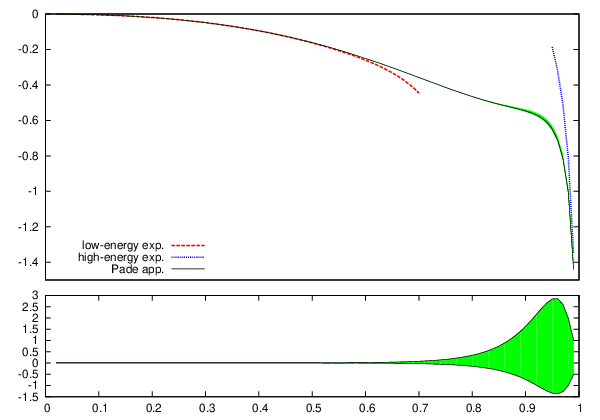
Refer to caption — Figure 1: Padé approximation for $\Pi^{(4)}\left(-\frac{x^{2}}{1-x}m_{\mu}^{2}\right)$ with muon loops. We show in the top half the approximants and in the bottom half the relative error with respect to the local mean of all approximants obtained.

At the top of the figure we show the envelope of all Padé approximants that have been calculated and compare with the low- and high-energy expansions. In the bottom half we show the maximal deviation from the mean in percent. As can be seen there are only significant deviations of the order of a few percent in the range $x>0.8$ , which correspond to the uncertainty due to a limited number of terms in the high-energy expansion.

2.4.2 Modifications at three loops

At three loops much deeper expansions can be used for the construction of the Padé approximants. The 30 known coefficients in the low-energy expansion [53, 54] together with 31 coefficients from the high-energy expansion [55] and three coefficients in the threshold expansion lead to a significantly larger system of constraints compared to the four-loop case.

Our strategy will be to incorporate as much of the threshold information as possible into the logarithmic function $\Pi^{(3)}_{\text{log}}(z)$ , so that all constraints are imposed at $\omega=0$ . The resulting system can be solved very efficiently using well-established techniques of one-point Padé approximation¹¹ 1 One-point approximation means that the value of the approximated function and its derivatives at a single point are known..

As in the four-loop case we first split the polarization function into two parts, using

$\displaystyle\Pi^{(3)}_{\text{log}}(z)=$	$\displaystyle\sum_{i\geq 0,j}k_{ij}{\cal K}^{(3)}_{ij}(z)+\sum_{m,n}d_{mn}{\cal D}^{(3)}_{mn}(z)\,,$	(29)
$\displaystyle{\cal K}^{(3)}_{ij}(z)=$	$\displaystyle\Pi^{(2)}(z)^{i}\*G(z)^{j}\times\begin{cases}(1-z)^{j}&\text{for }j>0\\ \quad 1&\text{otherwise}\end{cases}\,,$	(30)
$\displaystyle{\cal D}^{(3)}_{ij}(z)=$	$\displaystyle\big(z\,\G(z)\big)^{m}\\left(1-1/z\right)^{\lceil\frac{m}{2}\rceil}\frac{1}{z^{n}}$	(31)

to absorb the logarithms and the threshold singularity. Since we expect to obtain sufficiently many different Padé approximants for a reliable error estimate we refrain from introducing additional parameters at this point.

To map all available information from the low- and high-energy expansions onto $\omega=0$ , we define

	$\displaystyle P_{30}(\omega)$	$\displaystyle=z(\omega)^{31}\*\left(\Pi^{(3)}_{\text{reg}}\big(z(\omega)\big)-\sum_{i=0}^{30}\frac{H^{(3)}_{i}}{z(\omega)^{i}}\right)\,,$
	$\displaystyle H^{(3)}_{i}$	$\displaystyle=\frac{1}{i!}\left(\frac{\partial}{\partial(1/z)}\right)^{i}\Pi^{(3)}_{\text{reg}}(z)\Bigg\|_{z\to-\infty}\,.$		(32)

The Taylor approximant is fixed by imposing

p^{(i)}_{61,0}(0)=P^{(i)}_{30}(0)\,,\qquad i=0,\dots,61\,.

(33)

We can deduce all further approximants with $n+m=61$ and $n+m=60$ using Baker’s recursion formula [56]²² 2 Note that the denominator in the first equation of Eq. (13) in Ref. [56] contains an obvious typo. The proper expression is $\bar{\eta}_{2j-1}\*\theta_{2j-2}(x)-x\*\bar{\eta}_{2j-2}\*\theta_{2j-1}(x)$ .

	$\displaystyle p_{n-\frac{j}{2},\frac{j}{2}}$	$\displaystyle=\frac{\hat{\eta}_{j}}{\hat{\theta}_{j}}=\frac{\hat{\eta}_{j-2}-\omega\\,\hat{\eta}_{j-1}}{\hat{\theta}_{j-2}-\omega\\,\hat{\theta}_{j-1}}$	$\displaystyle j\text{ even}\,,$		(34)
	$\displaystyle p_{n-\frac{j+1}{2},\frac{j-1}{2}}$	$\displaystyle=\frac{\hat{\eta}_{j}}{\hat{\theta}_{j}}=\frac{\hat{\eta}_{j-2}-\hat{\eta}_{j-1}}{\hat{\theta}_{j-2}-\hat{\theta}_{j-1}}$	$\displaystyle j\text{ odd}\,,$		(35)

where the numerator $\hat{\eta}_{j}$ of the Padé approximant is normalised as in Eq. (27).

It should be noted that the known threshold constant at order $1-z$ is not included in the approximants. We find however that the information from the threshold region has virtually no effect on the reconstructed polarization functions in the Euclidean regime $z<0$ .³³ 3 If not all constraints from the low- and high-energy regions are taken into account, the importance of the threshold information increases. Still, not taking into account any threshold coefficients changes the polarization function by less than one per mille in the euclidean region, even if only three terms each from the low- and the high-energy expansion are taken into account. This is contrary to the four-loop case, where the approximants are far less constrained by the low- and high-energy expansions.

3 The anomalous magnetic moment of the muon at five loops

The QED corrections to the anomalous magnetic moment can be calculated in perturbation theory and can thus be written in form of a power series in the fine structure constant $\alpha$

a_{\mu}=\sum_{k=1}^{\infty}\left(\frac{\alpha}{\pi}\right)^{k}a_{\mu}^{(2k)}\,,

(36)

where $a_{\mu}^{(2k)}$ can be further decomposed – following the conventions in Ref. [8] – as

a_{\mu}^{(2k)}=A_{1}^{(2k)}+A_{2}^{(2k)}(m_{e}/m_{\mu})+A_{2}^{(2k)}(m_{\tau}/m_{\mu})+A_{3}^{(2k)}(m_{e}/m_{\mu},m_{\tau}/m_{\mu})\,.

(37)

$A_{1}^{(2k)}$ contains the universal contributions, which in case of the muon anomalous magnetic moment only contain muon loops. The diagrams contributing to $A_{2}^{(2k)}(m_{e}/m_{\mu})$ and $A_{2}^{(2k)}(m_{\tau}/m_{\mu})$ have at least one electron or tau loop, respectively. In $A_{3}^{(2k)}(m_{e}/m_{\mu},m_{\tau}/m_{\mu})$ contributions from diagrams with both electron and tau loops are collected. In this paper we are mainly interested in contributions to $A_{2}^{(2k)}(m_{e}/m_{\mu})$ without any muon loops.

The contributions to the anomalous magnetic moment of the muon due to photon polarization effects can be calculated (cf. Fig. 2) by using [10]

a_{\mu}=\frac{\alpha}{\pi}\int_{0}^{1}\mathrm{d}x(1-x)\frac{1}{1+\Pi(s_{x})}\,,\,s_{x}=-\frac{x^{2}}{1-x}m_{\mu}^{2}\,.

(38)

This formula can be obtained by considering the one-loop result for $g-2$ for the case of a heavy photon in combination with the dispersion relation for $\Pi(q^{2})$ . The right-hand side of Eq. (38) should be expanded in $\alpha$ , leading to e.g. at two-loop order

a_{\mu}^{(6)}=\int_{0}^{1}\mathrm{d}x(1-x)\left[-\Pi^{(2)}(s_{x})+\big(-\Pi^{(1)}(s_{x})\big)^{2}\right]\,.

(39)

The classes of diagrams accessible by this method are shown in Fig. 3.

	this work	Ref. [18]	Refs. [57, 58, 22, 59]
I(a)	20.142 813	20.183 2	20.142 93(23)	[57]
I(b)	27.690 061	27.718 8	27.690 38(30)	[57]
I(c)	4.742 149	4.817 59	4.742 12(14)	[57]
I(d)+I(e)	6.241 470	6.117 77	6.243 32(101)(70)	[57]
I(e)	-1.211 249	-1.331 41	-1.208 41(70)	[57]
I(f)+I(g)+I(h)	$\mbox{\phantom{0}4.446 8}{{\scriptstyle+6}\atop{\scriptstyle-4}}$	4.391 31	4.446 68(9)(23)(59)	[57, 58]
I(i)	$\mbox{\phantom{0}0.074 6}{{\scriptstyle+8}\atop{\scriptstyle-19}}$	0.252 37	0.087 1(59)	[22]
I(j)	$\mbox{-1.246 9}{{\scriptstyle+4}\atop{\scriptstyle-3}}$	-1.214 29	-1.247 26(12)	[59]

Table 1: Results for

A_{2}^{(10)}(m_{e}/m_{\mu})

with pure electronic insertions. The errors listed in the second column are estimated from the spread between different Padé approximants, which is negligible for classes I(a)–I(e). Please note that the authors of Ref. [18] only used the asymptotic form of

\Pi(s)

and did not provide any error estimate.

	this work	Ref. [8]
I(a)	22.566 976	22.566 973 (3)
I(b)	30.667 093	30.667 091 (3)
I(c)	5.141 395	5.141 395 (1)
I(e)	-0.931 839	-0.931 2 (24)

Table 2: Results for

A_{2}^{(10)}(m_{e}/m_{\mu})

including electronic and muonic contributions.

	this work	Ref. [9]
I(a)	0.000 471	0.000 470 94 (6)
I(b)	0.007 010	0.007 010 8 (7)
I(c)	0.023 467	0.023 468 (2)
I(d)+I(e)	0.014 094	0.014 098(5)(4)
I(e)	0.010 291	0.010 296 (4)
I(f)+I(g)+I(h)	$\mbox{0.037 85}{{\scriptstyle+5}\atop{\scriptstyle-3}}$	0.037 833(20)(6)(13)
I(i)	$\mbox{0.017 21}{{\scriptstyle+8}\atop{\scriptstyle-23}}$	0.017 47 (11)
I(j)	$\mbox{0.000 420}{{\scriptstyle+31}\atop{\scriptstyle-16}}$	0.000 397 5 (18)

Table 3: Results for the universal contributions

A_{1}^{(10)}

In the following, we compare the results obtained in our analysis with results from previous calculations. The numbers shown are obtained by numerically integrating over the best available approximation. In case there are several equivalent approximations the result is obtained by taking the mean of all values obtained. The errors are then calculated by taking the difference between the mean and the smallest and largest values obtained, respectively.

For classes I(a)–I(j) we present our results for the case of purely electronic vacuum polarization insertions in Tab. 1. We compare our results with the values obtained in Ref. [18], which relies only on the leading asymptotics of $\Pi(q^{2})$ , and results obtained by purely numerical calculations.

Since the results for classes I(a)-I(c) are obtained by numerical integrating the exact analytical expression for the one- and two-loop vacuum polarization they are exact.

In the case of classes I(d) and I(e) the used three-loop Padés are highly constrained by a large number of terms in the low- and high-energy expansion. Thus the error from the spread between different approximants is negligible. As can be seen the results are in good agreement with the results obtained in Ref. [57] and the analysis in Ref. [18] can clearly be improved by including sub-leading contributions.

In case of classes I(f)-I(j) the used four-loop Padés are less precise but also here we find good agreement within the quoted errors with the results obtained in Ref. [8]. In all cases one finds a significant improvement when comparing to the leading logarithmic approximation used in Ref. [18].

For classes I(a)-I(c) and I(e) we can obtain the full result for $A_{2}^{(10)}(m_{e}/m_{\mu})$ including muonic contributions. These results are presented in Tab. 2. In Tab. 3 we present our results for the universal corrections and compare with the results given in Ref. [9]. In both cases the discussion as for the purely electronic contributions can essentially be repeated and also here overall good agreement with results available in the literature is observed. Nevertheless it should be noted that for single diagram classes a certain tension remains.

As a check of our setup we repeated the analysis of Ref. [16] and find good agreement even though in that reference a term in the threshold region proportional to $\log^{2}(1-z)$ has been omitted (cf. Eq. (12)). Our findings at four-loop order are summarized in Tab. 4.

	this work	Ref. [16]	Ref. [8, 60]
I(c)	1.440741	–	1.440744(16) [60]
I(d)	-0.230337	-0.230362(5)	-0.22982(37) [8]

Table 4: Comparison of four-loop results for

A_{2}^{(8)}(m_{e}/m_{\mu})

obtained in Refs. [16, 8] and in this work. The classification of the diagrams corresponds to the notation used in Ref. [8].

4 Conclusions

We presented results for a certain set of five-loop contributions to the anomalous magnetic moment of the muon that stem from corrections to the vacuum polarization of the photon. We have shown that an improved treatment of the vacuum polarization, including more than its asymptotic form, leads to a significantly better agreement with results obtained by purely numerical methods. It can be clearly seen that for certain classes of diagrams the asymptotic form of the vacuum polarization function is not sufficient and power suppressed terms play an important role and have to be included in the analysis.

Acknowledgements

We like to thank K.G. Chetyrkin and J.H. Kühn for initiating the project, fruitful discussions, and reading of the manuscript. In addition, we thank K.G. Chetyrkin for valuable advice on computing the vacuum polarization function in high-energy limit. The work of P.B. was supported by RFBR grant 11-02-01196. P.M. has been supported in part by DFG Sonderforschungsbereich Transregio 9, Computergestützte Theoretische Teilchenphysik, and by the EU Network LHCPHENOnet PITN-GA-2010-264564.

References

[1] J. S. Schwinger, On quantum electrodynamics and the magnetic moment of the electron, Phys.Rev. 73 (1948) 416–417. doi:10.1103/PhysRev.73.416.
[2] A. Petermann, Fourth order magnetic moment of the electron, Helv.Phys.Acta 30 (1957) 407–408.
[3] C. M. Sommerfield, Magnetic dipole moment of the electron, Phys.Rev. 107 (1957) 328–329. doi:10.1103/PhysRev.107.328.
[4] T. Kinoshita, New value of the $\alpha^{3}$ electron anomalous magnetic moment, Phys.Rev.Lett. 75 (1995) 4728–4731. doi:10.1103/PhysRevLett.75.4728.
[5] S. Laporta, E. Remiddi, The analytical value of the electron (g-2) at order $\alpha^{3}$ in QED, Phys.Lett. B379 (1996) 283–291. arXiv:hep-ph/9602417, doi:10.1016/0370-2693(96)00439-X.
[6] K. Melnikov, T. v. Ritbergen, The three loop relation between the $\overline{\text{MS}}$ and the pole quark masses, Phys.Lett. B482 (2000) 99–108. arXiv:hep-ph/9912391, doi:10.1016/S0370-2693(00)00507-4.
[7] P. Marquard, L. Mihaila, J. Piclum, M. Steinhauser, Relation between the pole and the minimally subtracted mass in dimensional regularization and dimensional reduction to three-loop order, Nucl.Phys. B773 (2007) 1–18. arXiv:hep-ph/0702185, doi:10.1016/j.nuclphysb.2007.03.010.
[8] T. Aoyama, M. Hayakawa, T. Kinoshita, M. Nio, Complete tenth-order QED contribution to the muon g-2, Phys.Rev.Lett. 109 (2012) 111808. arXiv:1205.5370, doi:10.1103/PhysRevLett.109.111808.
[9] T. Aoyama, M. Hayakawa, T. Kinoshita, M. Nio, Tenth-order QED contribution to the electron g-2 and an improved value of the fine structure constant, Phys.Rev.Lett. 109 (2012) 111807. arXiv:1205.5368, doi:10.1103/PhysRevLett.109.111807.
[10] B. Lautrup, E. de Rafael, The anomalous magnetic moment of the muon and short-distance behaviour of quantum electrodynamics, Nucl.Phys. B70 (1974) 317–350. doi:10.1016/0550-3213(74)90481-7.
[11] T. Kinoshita, H. Kawai, Y. Okamoto, Asymptotic photon propagator in massive QED and the muon anomalous magnetic moment, Phys.Lett. B254 (1991) 235–240. doi:10.1016/0370-2693(91)90427-R.
[12] H. Kawai, T. Kinoshita, Y. Okamoto, Asymptotic photon propagator and higher order QED Callan-Symanzik beta function, Phys.Lett. B260 (1991) 193–198. doi:10.1016/0370-2693(91)90990-8.
[13] R. Faustov, A. Kataev, S. Larin, V. Starshenko, The analytical contribution of the three loop diagrams with two fermion circles to the photon propagator and the muon anomalous magnetic moment, Phys.Lett. B254 (1991) 241–246. doi:10.1016/0370-2693(91)90428-S.
[14] A. Kataev, Renormalization group and the five loop QED asymptotic contributions to the muon anomaly, Phys.Lett. B284 (1992) 401–409. doi:10.1016/0370-2693(92)90452-A,10.1016/j.physletb.2012.02.057.
[15] D. J. Broadhurst, A. Kataev, O. Tarasov, Analytical on-shell QED results: Three loop vacuum polarization, four loop $\beta$ function and the muon anomaly, Phys.Lett. B298 (1993) 445–452. arXiv:hep-ph/9210255, doi:10.1016/0370-2693(93)91849-I.
[16] P. Baikov, D. J. Broadhurst, Three loop QED vacuum polarization and the four loop muon anomalous magnetic moment arXiv:hep-ph/9504398.
[17] S. Laporta, The analytical contribution of some eighth order graphs containing vacuum polarization insertions to the muon (g-2) in QED, Phys.Lett. B312 (1993) 495–500. arXiv:hep-ph/9306324, doi:10.1016/0370-2693(93)90988-T.
[18] P. Baikov, K. Chetyrkin, J. Kühn, C. Sturm, The relation between the QED charge renormalized in $\overline{\text{MS}}$ and on-shell schemes at four loops, the qed on-shell $\beta$ -function at five loops and asymptotic contributions to the muon anomaly at five and six loops, Nucl.Phys. B867 (2013) 182–202. arXiv:1207.2199, doi:10.1016/j.nuclphysb.2012.09.018.
[19] R. Lee, P. Marquard, A. V. Smirnov, V. A. Smirnov, M. Steinhauser, Four-loop corrections with two closed fermion loops to fermion self energies and the lepton anomalous magnetic moment, JHEP 1303 (2013) 162. arXiv:1301.6481, doi:10.1007/JHEP03(2013)162.
[20] F. Jegerlehner, A. Nyffeler, The muon g-2, Phys.Rept. 477 (2009) 1–110. arXiv:0902.3360, doi:10.1016/j.physrep.2009.04.003.
[21] R. Barbieri, E. Remiddi, Electron and Muon 1/2(g-2) from Vacuum Polarization Insertions, Nucl.Phys. B90 (1975) 233. doi:10.1016/0550-3213(75)90645-8.
[22] T. Aoyama, M. Hayakawa, T. Kinoshita, M. Nio, Proper eighth-order vacuum-polarization function and its contribution to the tenth-order lepton g-2, Phys.Rev. D83 (2011) 053003. arXiv:1012.5569, doi:10.1103/PhysRevD.83.053003.
[23] A. Maier, P. Maierhöfer, P. Marquard, A. Smirnov, Low energy moments of heavy quark current correlators at four loops, Nucl.Phys. B824 (2010) 1–18. arXiv:0907.2117, doi:10.1016/j.nuclphysb.2009.08.011.
[24] P. Nogueira, Automatic feynman graph generation, J. Comput. Phys. 105 (1993) 279–289.
[25] T. Seidensticker, Automatic application of successive asymptotic expansions of Feynman diagrams arXiv:hep-ph/9905298.
[26] R. Harlander, T. Seidensticker, M. Steinhauser, Complete corrections of ${\cal O}(\alpha\alpha_{s})$ to the decay of the $Z$ boson into bottom quarks, Phys.Lett. B426 (1998) 125–132. arXiv:hep-ph/9712228, doi:10.1016/S0370-2693(98)00220-2.
[27] J. Vermaseren, New features of FORM. arXiv:math-ph/0010025.
[28] P. Marquard, D. Seidel, Crusher, unpublished.
[29] S. Laporta, High precision calculation of multiloop Feynman integrals by difference equations, Int.J.Mod.Phys. A15 (2000) 5087–5159. arXiv:hep-ph/0102033, doi:10.1016/S0217-751X(00)00215-7.
[30] K. Chetyrkin, M. Faisst, C. Sturm, M. Tentyukov, $\epsilon$ -finite basis of master integrals for the integration-by-parts method, Nucl.Phys. B742 (2006) 208–229. arXiv:hep-ph/0601165, doi:10.1016/j.nuclphysb.2006.02.030.
[31] Y. Schröder, A. Vuorinen, High-precision epsilon expansions of single-mass-scale four-loop vacuum bubbles, JHEP 0506 (2005) 051. arXiv:hep-ph/0503209, doi:10.1088/1126-6708/2005/06/051.
[32] Y. Schröder, M. Steinhauser, Four-loop decoupling relations for the strong coupling, JHEP 0601 (2006) 051. arXiv:hep-ph/0512058, doi:10.1088/1126-6708/2006/01/051.
[33] S. Laporta, High precision $\epsilon$ expansions of massive four loop vacuum bubbles, Phys.Lett. B549 (2002) 115–122. arXiv:hep-ph/0210336, doi:10.1016/S0370-2693(02)02910-6.
[34] K. Chetyrkin, J. H. Kühn, P. Mastrolia, C. Sturm, Heavy-quark vacuum polarization: First two moments of the ${\cal O}(\alpha_{s}^{3}n_{f}^{2})$ contribution, Eur.Phys.J. C40 (2005) 361–366. arXiv:hep-ph/0412055, doi:10.1140/epjc/s2005-02151-y.
[35] B. A. Kniehl, A. V. Kotikov, Calculating four-loop tadpoles with one non-zero mass, Phys.Lett. B638 (2006) 531–537. arXiv:hep-ph/0508238, doi:10.1016/j.physletb.2006.04.057.
[36] Y. Schröder, M. Steinhauser, Four-loop singlet contribution to the electroweak $\rho$ parameter, Phys.Lett. B622 (2005) 124–130. arXiv:hep-ph/0504055, doi:10.1016/j.physletb.2005.06.085.
[37] E. Bejdakic, Y. Schröder, Hypergeometric representation of a four-loop vacuum bubble, Nucl.Phys.Proc.Suppl. 160 (2006) 155–159. arXiv:hep-ph/0607006, doi:10.1016/j.nuclphysbps.2006.09.040.
[38] B. A. Kniehl, A. V. Kotikov, Heavy-quark QCD vacuum polarisation function: Analytical results at four loops, Phys.Lett. B642 (2006) 68–71. arXiv:hep-ph/0607201, doi:10.1016/j.physletb.2006.09.008.
[39] B. Kniehl, A. Kotikov, A. Onishchenko, O. Veretin, Strong-coupling constant with flavor thresholds at five loops in the modified minimal-subtraction scheme, Phys.Rev.Lett. 97 (2006) 042001. arXiv:hep-ph/0607202, doi:10.1103/PhysRevLett.97.042001.
[40] P. Baikov, A Practical criterion of irreducibility of multi-loop Feynman integrals, Phys.Lett. B634 (2006) 325–329. arXiv:hep-ph/0507053, doi:10.1016/j.physletb.2006.01.052.
[41] P. Baikov, Explicit solutions of the three loop vacuum integral recurrence relations, Phys.Lett. B385 (1996) 404–410. arXiv:hep-ph/9603267, doi:10.1016/0370-2693(96)00835-0.
[42] P. Baikov, K. Chetyrkin, Four loop massless propagators: An algebraic evaluation of all master integrals, Nucl.Phys. B837 (2010) 186–220. arXiv:1004.1153, doi:10.1016/j.nuclphysb.2010.05.004.
[43] A. Smirnov, M. Tentyukov, Four loop massless propagators: a numerical evaluation of all master integrals, Nucl.Phys. B837 (2010) 40–49. arXiv:1004.1149, doi:10.1016/j.nuclphysb.2010.04.020.
[44] A. Hoang, M. Beneke, K. Melnikov, T. Nagano, A. Ota, et al., Top - anti-top pair production close to threshold: Synopsis of recent NNLO results, Eur.Phys.J.direct C2 (2000) 1. arXiv:hep-ph/0001286.
[45] A. H. Hoang, V. Mateu, S. Mohammad Zebarjad, Heavy Quark Vacuum Polarization Function at ${\cal O}(\alpha_{s}^{2})$ and ${\cal O}(\alpha_{s}^{3})$ , Nucl. Phys. B813 (2009) 349–369. arXiv:0807.4173, doi:10.1016/j.nuclphysb.2008.12.005.
[46] Y. Kiyo, A. Maier, P. Maierhöfer, P. Marquard, Reconstruction of heavy quark current correlators at ${\cal O}(\alpha_{s}^{3})$ , Nucl.Phys. B823 (2009) 269–287. arXiv:0907.2120, doi:10.1016/j.nuclphysb.2009.08.010.
[47] G. A. Baker, Essentials of Padé Approximants, Academic Press, Inc., 1975.
[48] D. J. Broadhurst, J. Fleischer, O. V. Tarasov, Two loop two point functions with masses: Asymptotic expansions and Taylor series, in any dimension, Z. Phys. C60 (1993) 287–302. arXiv:hep-ph/9304303, doi:10.1007/BF01474625.
[49] J. Fleischer, O. V. Tarasov, Calculation of Feynman diagrams from their small momentum expansion, Z. Phys. C64 (1994) 413–426. arXiv:hep-ph/9403230, doi:10.1007/BF01560102.
[50] D. J. Broadhurst, et al., Two loop gluon condensate contributions to heavy quark current correlators: Exact results and approximations, Phys. Lett. B329 (1994) 103–110. arXiv:hep-ph/9403274, doi:10.1016/0370-2693(94)90524-X.
[51] K. G. Chetyrkin, J. H. Kühn, M. Steinhauser, Heavy Quark Vacuum Polarisation to Three Loops, Phys. Lett. B371 (1996) 93–98. arXiv:hep-ph/9511430, doi:10.1016/0370-2693(95)01593-0.
[52] K. Chetyrkin, J. H. Kühn, M. Steinhauser, Three loop polarization function and ${\cal O}(\alpha_{s}^{2})$ corrections to the production of heavy quarks, Nucl.Phys. B482 (1996) 213–240. arXiv:hep-ph/9606230, doi:10.1016/S0550-3213(96)00534-2.
[53] R. Boughezal, M. Czakon, T. Schutzmeier, Four-Loop Tadpoles: Applications in QCD, Nucl.Phys.Proc.Suppl. 160 (2006) 160–164. arXiv:hep-ph/0607141, doi:10.1016/j.nuclphysbps.2006.09.041.
[54] A. Maier, P. Maierhöfer, P. Marquard, Higher moments of heavy quark correlators in the low energy limit at ${\cal O}(\alpha_{s}^{2})$ , Nucl.Phys. B797 (2008) 218–242. arXiv:0711.2636, doi:10.1016/j.nuclphysb.2007.12.035.
[55] A. Maier, P. Marquard, Low- and high-energy expansion of heavy-quark correlators at next-to-next-to-leading order, Nucl.Phys. B859 (2012) 1–12. arXiv:1110.5581, doi:10.1016/j.nuclphysb.2012.01.021.
[56] G. A. Baker Jr., J. L. Gammel, The Padé Approximant in Theoretical Physics, Vol. 71 of Mathematics in Science and Engineering, Academic Press, Inc., 1970, Ch. 1, pp. 1–38.
[57] T. Kinoshita, M. Nio, The tenth-order qed contribution to the lepton g-2: Evaluation of dominant $\alpha^{5}$ terms of muon g-2, Phys.Rev. D73 (2006) 053007. arXiv:hep-ph/0512330, doi:10.1103/PhysRevD.73.053007.
[58] T. Aoyama, M. Hayakawa, T. Kinoshita, M. Nio, Tenth-order lepton anomalous magnetic moment: Second-order vertex containing two vacuum polarization subdiagrams, one within the other, Phys.Rev. D78 (2008) 113006. arXiv:0810.5208, doi:10.1103/PhysRevD.78.113006.
[59] T. Aoyama, M. Hayakawa, T. Kinoshita, M. Nio, N. Watanabe, Eighth-order vacuum-polarization function formed by two light-by-light-scattering diagrams and its contribution to the tenth-order electron g-2, Phys.Rev. D78 (2008) 053005. arXiv:0806.3390, doi:10.1103/PhysRevD.78.053005.
[60] T. Kinoshita, M. Nio, Improved alpha**4 term of the muon anomalous magnetic moment, Phys.Rev. D70 (2004) 113001. arXiv:hep-ph/0402206, doi:10.1103/PhysRevD.70.113001.

$\displaystyle\Pi^{(4)}_{\text{thr},-2}=$	$\displaystyle\frac{1}{128}\\pi^{2}\\zeta_{3}\*n_{l}\,,$	(14)
$\displaystyle\Pi^{(4)}_{\text{thr},-1}=$	$\displaystyle\bigg(\frac{7}{2304}\\pi^{3}-\frac{11}{384}\\pi^{3}\a_{1}-\frac{11}{64}\\pi\\zeta_{3}\bigg)\n_{l}-\frac{11}{768}\\pi^{3}\n_{l}\*\log(1-z)\,,$	(15)
$\displaystyle\Pi^{(4)}_{\text{thr},0}=$	$\displaystyle\bigg(-\frac{467}{18432}+\frac{115}{384}\a_{1}-\frac{121}{256}\a_{1}^{2}-\frac{2207}{9216}\\pi^{2}+\frac{5}{48}\\pi^{2}\*a_{1}$
	$\displaystyle+\frac{9}{4096}\\pi^{4}+\frac{131\\zeta_{3}}{512}\bigg)\n_{l}\\log(1-z)$
	$\displaystyle+\bigg(-\frac{839}{9216}+\frac{\pi^{2}}{144}\bigg)\n_{l}^{2}\\log(1-z)$
	$\displaystyle+\bigg(\frac{115}{1536}-\frac{121}{512}\a_{1}+\frac{11}{768}\\pi^{2}\bigg)\n_{l}\\log^{2}(1-z)$
	$\displaystyle-\frac{121}{3072}\n_{l}\\log^{3}(1-z)+\text{const}\,,$	(16)