A Dynamic Learning Algorithm for Online Matching Problems with Concave Returns
Abstract
We consider an online matching problem with concave returns. This problem is a generalization of the traditional online matching problem and has vast applications in online advertising. In this work, we propose a dynamic learning algorithm that achieves near-optimal performance for this problem when the inputs arrive in a random order and satisfy certain conditions. The key idea of our algorithm is to learn the input data pattern dynamically: we solve a sequence of carefully chosen partial allocation problems and use their optimal solutions to assist with the future decisions. Our analysis belongs to the primal-dual paradigm; however, the absence of linearity of the objective function and the dynamic feature of the algorithm makes our analysis quite unique. We also show through numerical experiments that our algorithm performs well for test data.
keywords
online algorithms; primal-dual; dynamic price update; random permutation model; Adwords problem1 Introduction
In traditional optimization models, inputs are usually assumed to be known and efficient algorithms are sought to find the optimal solutions. However, in many practical cases, data does not reveal itself at the beginning. Instead, it comes in an online fashion. For example, in many revenue management problems, customers arrive sequentially and each time a customer arrives, the decision maker has to make some irrevocable decisions (e.g., what product to sell, at what prices) for this customer without knowing any of the future inputs. Such a regime is often called online optimization. Online optimization has gained much attention in the research community in the past few decades due to its applicability in many practical problems, and much effort has been directed toward understanding the quality of solutions that can be obtained under such settings. For an overview of the online optimization literature and its recent developments, we refer the readers to Borodin and El-Yaniv (1998), Buchbinder and Naor (2009) and Devanur (2011).
In this paper, we consider a special type of online optimization problem - an online matching problem. Online matching problems are considered as fundamental problems in online optimization theory and have important applications in the online advertisement allocation problems. For a review of online matching problems, we refer the readers to Mehta (2012). In the problem we study, there is an underlying weighted bipartite graph with weights for each edge . The vertices in arrive sequentially in some order, and whenever a vertex arrives, the set of weights is revealed for all , . The decision maker then has to match to one of its neighbors , and a value of will be obtained from this matching. In our problem, the decision maker’s gain from each vertex is a function of the total matched value to this vertex, and his goal is to maximize the total gain from all vertices. Mathematically, the problem can be formulated as follows (assume , , and let for ):
| (1) |
where denotes the fraction of vertex that is matched to vertex .11 1 We allow fractional allocations in our model. However, our proposed algorithms output integer solutions. Thus all our results hold if one confines to integer solutions. In (1), the coefficient is revealed only when vertex arrives, and an irrevocable decision has to be made before observing the next input. For each , is a nondecreasing concave function with . In this paper, we assume that s are continuously differentiable.
As mentioned earlier, online matching problems have a very important application in the online advertisement allocation problem, which we will later refer to as the Adwords problem. In the Adwords problem, there are advertisers (which we also call the bidders). A sequence of keywords are searched during a fixed time horizon. Based on the relevance of the keyword, the th bidder would bid a certain amount to show his advertisement on the result page of the th keyword. The search engine’s decision is to allocate each keyword to one of the bidders (we only consider a single allocation in this paper). Note that each allocation decision can only depend on the information earlier in the arrival sequence but not on any future data. As pointed out in Devanur and Jain (2012), there are several practical motivations for considering a concave function of the matched bids in the Adwords problem. Among them are convex penalty costs for under-delivery in search engine-advertiser contracts, the concavity of the click-through rate in the number of allocated bids observed in empirical data and fairness considerations. In each of the situations mentioned above, one can write the objective as a concave function. We refer the readers to Devanur and Jain (2012) for a more thorough review of the motivations for this problem. It is worth noting that there is a special case of this problem where . In this case, one can view that the bidder has a budget and the revenue from each bidder is bounded by .
One important question when studying online algorithms is the assumptions on the input data. In this work, we adopt a random permutation model. More precisely, we assume:
- 1.
The total number of arrivals is known a priori.
- 2.
The weights can be adversarially chosen. However, the order that arrives is uniformly distributed over all the permutations.
The random permutation model has been adopted in much recent literature in the study of online matching problems, see, e.g., Devanur and Hayes (2009), Feldman et al. (2010), Agrawal et al. (2014), etc. It is equivalent to saying that a set of is arbitrarily chosen beforehand (unknown to the decision maker). Then the arrivals are drawn randomly without replacement from . The random permutation model is an intermediate path between using a worst-case analysis and assuming each input data is drawn independently and identically distributed (i.i.d.) from a certain distribution. On one hand, compared to the worst-case analysis (see, e.g., Mehta et al. 2005, Buchbinder et al. 2007, Feldman et al. 2009, Devanur and Jain 2012), the random permutation model is practically reasonable yet much less conservative. On the other hand, the random permutation model is much less restrictive than assuming the inputs are drawn i.i.d. from a certain distribution (Devanur 2011). Also, the assumption of the knowledge of is necessary for any online algorithm to achieve near-optimal performance (see Devanur and Hayes 2009). Therefore, for large problems with relatively stationary inputs, the random permutation model is a good approximation and the study of such models is of practical interest. Next we define the performance measure of an algorithm under the random permutation model:
Definition 1 (-competitiveness)
Let OPT be the optimal value for the offline problem (1). An online algorithm is called -competitive in the random permutation model if the expected value of the online solutions by using is at least times the optimal value of (1), that is
where the expectation is taken over uniformly random permutations of , and is the th decision made by algorithm when the inputs arrive in order .
In Devanur and Jain (2012), the authors propose an algorithm for the online matching problem with concave returns that has a constant competitive ratio under the worst-case model (the constant depends on the forms of each ). They also show that a constant competitive ratio is the best possible result under that model. In this paper, we propose an algorithm under the random permutation model, which achieves near-optimal performance under some conditions on the input.
Our main result is stated as follows:
Theorem 1
Fix . There exists an algorithm (Algorithm DLA) that is competitive for the online matching problem with concave returns s under the random permutation model if
| (2) |
where , , and is a constant that only depends on each and .
In condition (2), can be viewed as the average bid value of a bidder over time. Given that each bidder is at least interested in some fractions of the keywords, this average will go to a certain constant as becomes large. Also, can be viewed as the ratio between the value of the smallest non-zero bid and the highest bid. In practice, this is often bounded below by a constant by enforcing a reserve price and a maximum price for any single bid. The exact functional form of is somewhat complicated, and is given in Proposition 1. Just to give an example, if we choose (), then . Therefore, condition (2) can be viewed as simply requiring the total number of inputs is large, which is often the case in practice. For example, in the Adwords problem, is the number of keyword searches in a certain period, and for instance, Google receives more than billion searches per day. Even if we focus on a specific category, the number can still be in the millions. Thus, this condition is reasonable. We note that most learning algorithms in the literature make similar requirements, see Devanur and Hayes (2009), Agrawal et al. (2014), and Molinaro and Ravi (2014). Furthermore, as we will show in our numerical tests, our algorithm performs well even for problems with sizes that are significantly smaller than the condition requires, which validates the potential usefulness of our algorithm.
To propose an algorithm that achieves near-optimal performance, the main idea is to utilize the observed data in the allocation process. In particular, since the input data arrives in a random order, using the past input data and projecting it into the future should present a good approximation for the problem. To mathematically capture this idea, we use a primal-dual approach. We obtain the dual optimal solutions to suitably constructed optimization problems and use them to assist with future allocations. We first propose a one-time learning algorithm (OLA, see Section 2) that only solves an optimization problem once at time . By carefully examining this algorithm, we prove that it achieves near-optimal performance when the inputs satisfy certain conditions. However, the conditions are stronger than those stated in Theorem 1. To improve our algorithm, we further propose a dynamic learning algorithm (DLA, see Section 3). The dynamic learning algorithm makes better use of the observed data and updates the dual solution at a geometric pace, that is, at time , , and so on. We show that these resolvings can lift the performance of the algorithm and thus prove Theorem 1. As one will see in the proof of the DLA, the choice of the resolving points perfectly balances the trade-off between exploration and exploitation, which are the main trade-offs in such types of learning algorithms.
It is worth mentioning that a similar kind of dynamic learning algorithm has been proposed in Agrawal et al. (2014) and further studied in Wang (2012) and Molinaro and Ravi (2014). However, those works only focus on linear objectives. In our analysis, the nonlinearity of the objective function presents a non-trivial hurdle since one can no longer simply analyze the revenue generated in each time segment and add them together. In this paper, we successfully work around this hurdle by a convex duality argument. We believe that our analysis is a non-trivial extension of the previous work. Moreover, the problem solved has important applications.
The remainder of the paper is organized as follows. In Section 2, we start with a one-time learning algorithm and prove that it achieves near-optimal performance under some mild conditions on the input. The one-time learning algorithm is easy to understand and shows important insights for designing this class of learning algorithms. However, it only achieves a weaker performance than what is stated in Theorem 1. In Section 3, we propose a dynamic learning algorithm which makes better use of the data and has a stronger performance. Some numerical test results of our algorithm are presented in Section 4, which validate the strength of our algorithm. Section 5 concludes this paper.
2 One-Time Learning Algorithm
We first rewrite the offline problem (1) as follows:
| (3) |
We define the following dual problem:
| (4) |
Let the optimal value of (3) be and the optimal value of (4) be . In Devanur and Jain (2012), the authors proved the weak duality between (3) and (4). In the following lemma, we prove that in fact the strong duality holds. The proof of the lemma is relegated to the Appendix.
Lemma 1
. Furthermore, the objective value of any feasible solution to (4) is an upper bound of .
Before we describe our algorithm, we define the following partial optimization problem:
| (5) |
Now we define the one-time learning algorithm as follows:
- 1.
During the first arrivals, no allocation is made.
- 2.
After observing the first arrivals, solve () and denote the optimal solutions by and .
- 3.
For any dimensional vector , define
Here, ties among are broken arbitrarily. For the th to the th arrival, the allocation rule is used.
Now we provide some intuition for the algorithm. The idea of the algorithm is to use the first inputs to learn an approximate and then use it to make all the future allocations based on the complementarity conditions between the primal and dual problems ((3) and (4)). Here is solved from () which projects the allocation in the first inputs to the entire problem. The decision rule in (3) can be explained as choosing the with the highest product of the nominal bid value and the marginal contribution rate to the total projected reward . Note that a similar idea has been used to construct algorithms for an online matching problem with linear objective functions (see e.g., Devanur and Hayes 2009, Agrawal et al. 2014, Molinaro and Ravi 2014). However, the analyses of those algorithms all depend on the linearity of the objective function which we do not possess in this problem. Instead, an analysis with the use of concavity is required in our analysis, making it quite different from those in the prior literature. In the following, we assume without loss of generality that (we can always scale the inputs to make this hold). We also make a technical assumption as follows:
Assumption 1
The inputs of the problem are in a general position. That is, for any vector , there are at most terms among , , that are not singleton sets.
The assumption says that we only need to break ties in (3) no more than times. This assumption is not necessarily true for all inputs. However, as pointed out by Devanur and Hayes (2009) and Agrawal et al. (2014), one can always perturb by adding a random variable taking uniform distribution on for some very small . By doing so the assumption holds with probability one and the effect to the solution can be made arbitrarily small. Given this assumption and by the complementarity conditions, we have the following lemma, whose proof is in the Appendix.
Lemma 2
We first prove the following proposition about the performance of the OLA, which relies on a condition of the solution to ().
Proposition 1
For any given , if , then the OLA is a -competitive algorithm.
Before we prove Proposition 1, we define some notation.
- •
We define the optimal offline solution to (3) by with optimal value OPT.
- •
Define , note that normally does not equal .
We show the following lemma:
Lemma 3
For any given , if , then with probability ,
| (9) |
Proof. The proof will proceed as follows: For any fixed , we define that a random sample (the first arrivals) is bad for this if and only if is the optimal solution to (5) for this , but , or , for some . First, we show that the probability of a bad sample is small for every fixed (satisfying ) and . Then, we take a union bound over all distinct and s to prove the lemma.
To start with, we fix and . Define . By Lemma 2 and the condition on , we have
Therefore, the probability of bad is bounded by the sum of the following two terms ():
| (10) |
For the first term, we first define and we have
Then we have
Here the second inequality follows from the Hoeffding-Bernstein’s inequality for sampling without replacement, see Lemma 8 in the Appendix. Similarly, we can get the same result for the second term in (10), which is also bounded by . Therefore, the probability of a bad sample is bounded by for fixed and .
Next, we take a union bound over all distinct s. We call and distinct if and only if they result in different allocations, i.e., for some , . Denote . For each , by the definition in (3), the allocation is uniquely defined by the signs of the following terms:
There are such terms for each . Therefore, the entire
allocation profiles for all the arrivals can be determined by
the signs of no more than differences. Now we find out how
many different allocation profiles can arise by choosing different
s. By Orlik and Terao (1992), the total number of different profiles for
the differences can not exceed .
Therefore, the number of distinct s is no more than
. Now we take a union bound over all
distinct s and , and Lemma
3
follows.
Next we show that the OLA achieves a near-optimal solution under the condition in Proposition 1. We first construct a feasible solution to (4):
By Lemma 1, is an upper bound of OPT. Thus, we have
where the last equality is because by the allocation rule (3):
Now, we claim that if condition (9) holds,
We consider the following two cases:
- •
Case 1: . In this case,
where the second inequality holds because of the concavity of .
- •
Case 2: . In this case,
Again, the second inequality is due to the concavity of .
Thus, under the condition that , with probability ,
i.e., .
Lastly, we note that the actual allocation in our algorithm for is (since we ignore the first arrivals). By Lemma 2, we have
Thus when condition (9) holds, . Therefore,
The last inequality is due to the concavity of s and that . Therefore, given , with probability ,
Therefore, Proposition 1 is proved.
Proposition 1 shows that the OLA is near-optimal under some conditions on . However, is essentially an output of the algorithm. Although such types of conditions are not uncommon in the study of online algorithms (e.g., in the result of Devanur and Hayes 2009, Feldman et al. 2010), it is quite undesirable. In the following, we address this problem by providing a set of sufficient conditions which only depend on the input parameters (i.e., , , s and s). We show that our algorithm achieves near-optimal performance under these conditions. We start with the following lemma.
Lemma 4
For any , suppose the following condition holds:
| (11) |
where , and is such that
Then with probability , , for all .
The proof of Lemma 4 is relegated to the Appendix (it is proved together with Lemma 7). Now combining Proposition 1 and Lemma 4, we have the following result for the OLA:
Proposition 2
Fix any . Suppose
| (12) |
where , and is such that
| (13) |
with . Then the OLA is -competitive under the random permutation model.
Here we give some comments on the definition of . The definition of basically ensures that we rule out the possibility that one receives nearly all the allocation while some others receive almost none. Note that such always exists and is finite if for all . In practice, this is usually true as there is usually a upper bound on the possible reward from each bidder . In particular, if for all and , then one can choose
where denotes the inverse function of . For example, if one chooses (), then one can further choose . Therefore, in most practical situations, one can view as a constant. Finally, we want to remark that the conditions in Lemma 4 (or Proposition 2) are only one set of sufficient conditions which have the nice feature of only depending on the problem inputs. In practice, one can always resort to the condition in Proposition 1 () if they are more favorable. In addition, as we will show in our numerical tests in Section 4, our algorithm performs quite well even if some of the conditions in Lemma 4 are not satisfied. Therefore, the applicability of our algorithm could be well beyond what the conditions require.
3 Dynamic Learning Algorithm
In the previous section, we introduced the OLA that can achieve near-optimal performance. While the OLA illustrates the ideas of our approach and requires solving a convex optimization problem only once, the conditions it requires to achieve near-optimality are stricter than what we claim in Theorem 1. In this section, we propose an enhanced algorithm that lessens the conditions and thus improves the OLA.
The main idea for the enhancement is the following: In the one-time learning algorithm, we only solve a partial optimization problem once. However, it is possible that there is some error for that solution due to the random order of arrival. If we could modify the solution as we gather more data, we might be able to improve the performance of the algorithm. In the following, we introduce a dynamic learning algorithm based on this idea, which updates the allocation policy every time the history doubles; that is, it computes a new at time and uses it to perform the matching for the next time period. We define the following problem:
We further define to be the optimal solution to ().
We define the dynamic learning algorithm as follows:
- 1.
During the first arrivals, no allocation is made.
- 2.
For , for , set for all , where .
In the following, without loss of generality, we assume that is an integer (otherwise one can just choose a smaller and prove the same result). Define , , and define . We first prove the following proposition:
Proposition 3
If for all , , then the DLA is -competitive under the random permutation model.
Before we proceed to the proof, we first define some more notation. We define:
Note that in these definitions, is the allocated values for in the period to using , which is the actual allocation in that period. is the allocation for in all periods if is used. is the actual allocation for during the entire algorithm. We first prove the following lemma bounding the differences between , and .
Lemma 5
If , then with probability , for all ,
| (14) |
and
| (15) |
Lemma 5 shows that with high probability, , and are close to each other. In particular, when is small, the factor is relatively loose while as increases, the factor becomes tight. The proof of Lemma 5 is similar to that of Lemma 3 and is relegated to the Appendix.
The next lemma gives a bound on the revenue obtained by the DLA.
Lemma 6
If for all and , then with probability ,
The proof of Lemma 6 can be found in the Appendix.
Finally, we prove Proposition 3. We bound the objective value of the actual allocation. Note that the actual allocation for each can be written as
where . By the property of concave functions, we have
By Lemma 6, with probability
where the last inequality is because
Therefore, Proposition 3 is proved.
Similar to Lemma 4, we have the following conditions on the input parameters such that with high probability, the conditions in Proposition 3 hold.
Lemma 7
For any , suppose the following condition holds:
| (16) |
where , and is such that
Then with probability , , for all .
The proof of Lemma 7 is given in the Appendix. Finally, we combine Proposition 3 and Lemma 7, and Theorem 1 follows.
The same remark after Lemma 4 applies here. In particular, the conditions in Lemma 7 is only one set of sufficient conditions for our algorithm to achieve the target performance. However, one may also use the conditions in Proposition 3 if they turn out to hold in practice. In the next section, we show that the DLA works well even if the conditions in Lemma 7 are not satisfied.
4 Numerical Experiments
In this section, we report some numerical test results for our algorithms (both the OLA and the DLA). The objective is to validate the strength of our approaches and investigate the relationship between the performance of our algorithms and the input parameters.
In our numerical tests, we consider the Adwords problem. We assume there are advertisers (bidders), keywords arriving sequentially, and is the amount bidder would like to pay to display his advertisement on keyword search . We introduce a base problem in which we set , and with . The bidding values are generated in the following way:
- 1.
Assume there are categories of keywords. For each category , there is a base valuation of bidder , denoted by , which is generated according to the following distribution:
where denotes a uniformly distributed random variable on .
- 2.
For each arriving keyword, we first randomly choose a category. The probability for each category , denoted by , is randomly chosen on the simplex . Then if category is chosen, the final bid value for bidder will be .
Although the way is chosen seems arbitrary, we believe it reflects some major features of the bid values in practice. In the Adwords problem, each bidder is interested in certain categories of keywords. For example, a sport product company is interested in keywords related to sports. The s represent such interest levels. Then the bidder ’s actual bid on such a keyword is the base value multiplied by a random number, which reflects some level of idiosyncrasies of each keyword arrival. We also tested other ways to generate , and the test results are similar. We will report those test results in the end of this section.
To evaluate the performance of our algorithms, we introduce the notion of Relative Loss (RL) defined as follows:
In the numerical experiment, there is one key parameter we need to set in both of our algorithms: . In Theorem 1 and Proposition 1, we gave sufficient conditions on the inputs such that the algorithms will have expected RL less than . However, the theoretical results are asymptotic and thus may not represent the best practical choice of . In Table 1 and Figure 1, we first test both our OLA and DLA with different choices of . We have the following observations from Table 1 and Figure 1 (each number in Table 1 is the average of independent runs, the standard deviations of the results are insignificant compared to the average value):
- •
For the DLA, choosing a smaller improves its performance. There are two reasons for that. First, choosing a smaller reduces the loss due to ignoring the first bids. Second, it increases the number of price updates which help the decision maker to refine the decision policy and achieve better performance. Therefore one should choose a smaller in the DLA.
- •
For the OLA, the optimal choice of is more subtle. There are two countervailing forces when one chooses a smaller . On one hand, by choosing a smaller , the loss due to the failure to allocate any bid during period to becomes smaller, which benefits the algorithm. On the other hand, if is too small, the learned price may not be accurate enough which may lead to poor allocation in the remaining periods. In the test example, the optimal choice is .
- •
The DLA outperforms the OLA for all choices of .
| 0.001 | 0.005 | 0.01 | 0.02 | 0.05 | 0.10 | |
|---|---|---|---|---|---|---|
| OLA | 22.02% | 5.17% | 4.07% | 3.71% | 6.10% | 10.26% |
| DLA | 0.47% | 0.84% | 1.27% | 2.15% | 4.89% | 9.41% |

Next we focus ourselves on the DLA. As shown in Table 1, we prefer to choose a smaller in the DLA. In the following experiments, we will choose . Next we compare the performance of the DLA to a myopic allocation method which simply allocates each incoming keyword to the bidder with the highest value. We also study the impact of the two parameters, and , on the performance of our algorithm. We generate instances of the input and compare the average performance. The results of the average RL are shown in Table 2 (the standard deviations are shown in the parentheses) as well as in Figures 2(a) and 2(b).
| 1,000 | 2,000 | 5,000 | 10,000 | 20,000 | |
|---|---|---|---|---|---|
| DLA | 1.29% (0.29%) | 0.87% (0.26%) | 0.58% (0.12%) | 0.57% (0.17%) | 0.57% (0.16%) |
| Myopic | 3.07% (0.47%) | 3.03% (0.61%) | 2.90% (0.49%) | 3.11% (0.54%) | 2.96% (0.47%) |
| 0.5 | 0.6 | 0.7 | 0.8 | 0.9 | |
| DLA | 2.30% (0.82%) | 1.87% (0.67%) | 1.55% (0.56%) | 0.99 % (0.34%) | 0.57% (0.17%) |
| Myopic | 14.38% (2.01%) | 12.46% (1.81%) | 9.46% (1.38%) | 6.51% (1.05%) | 3.11% (0.54%) |
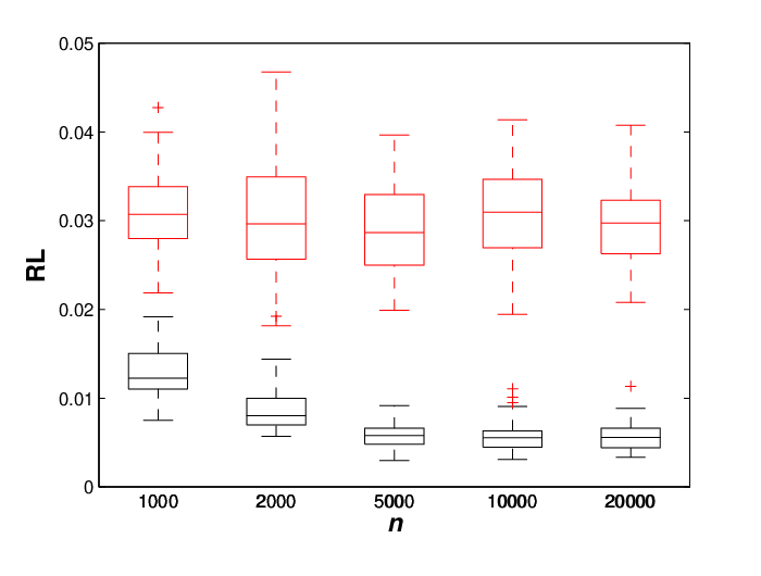
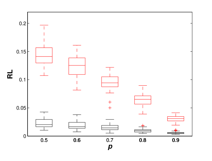
From Table 2, we can see that the DLA consistently performs better than the myopic approach. In particular, the performance of the DLA gradually improves when increases, while the performance of the myopic approach seems to be insensitive to the size of the problem. Moreover, even for small values of , the performance of the DLA is still very good. This means that the DLA works well even for problems whose size is much smaller than what Theorem 1 requires. For the parameter , we can see that both the DLA and the myopic algorithm deteriorate when decreases, but the DLA deteriorates much slower. Finally, we comment that these results are computed when we ignore the first bids. In practice, one does not need to do that and the performance of the DLA would be even better.
Finally, we repeat the above test for different setups of the inputs. We fix the parameters , and with in the base problem and generate s in the following ways:
- 1.
follows a normal distribution (truncated at and ). The parameters of each normal distribution (mean and standard deviation ) are randomly generated from a uniform distribution on .
- 2.
follows a Beta distribution. The parameters of the Beta distribution are generated from a uniform distribution on .
- 3.
follows a mixed normal and Beta distribution. That is, with probability , follows a truncated normal distribution with mean and standard deviation , and with probability , follows a Beta distribution with .
Next, we compare the performance of the DLA (choose ) and the myopic algorithm. For each case, we generate 100 instances of the input and compare the average RL. The results are shown in Table 3.
| Case 1 | 1,000 | 2,000 | 5,000 | 10,000 | 20,000 | |
| DLA | 1.56% (0.33%) | 0.84% (0.18%) | 0.36% (0.07%) | 0.21% (0.05%) | 0.14% (0.03%) | |
| Myopic | 1.45% (0.45%) | 1.37% (0.47%) | 1.42% (0.45%) | 1.41% (0.48%) | 1.31% (0.47%) | |
| 0.5 | 0.6 | 0.7 | 0.8 | 0.9 | ||
| DLA | 0.20% (0.04%) | 0.22% (0.06%) | 0.22% (0.05%) | 0.21% (0.03%) | 0.21% (0.05%) | |
| Myopic | 9.10% (2.01%) | 7.98% (2.00%) | 5.71% (1.32%) | 3.38% (0.96%) | 1.44% (0.46%) | |
| Case 2 | 1,000 | 2,000 | 5,000 | 10,000 | 20,000 | |
| DLA | 1.19% (0.24%) | 0.61% (0.12%) | 0.25% (0.08%) | 0.13% (0.07%) | 0.12% (0.08%) | |
| Myopic | 13.91% (2.07%) | 13.66% (2.48%) | 13.90% (2.07%) | 13.78% (1.97%) | 13.62% (2.12%) | |
| 0.5 | 0.6 | 0.7 | 0.8 | 0.9 | ||
| DLA | 0.20% (0.16%) | 0.29% (0.20%) | 0.21% (0.12%) | 0.17% (0.11%) | 0.13% (0.07%) | |
| Myopic | 40.57% (6.50%) | 38.30% (5.98%) | 32.45% (4.71%) | 24.67% (3.26%) | 13.46% (2.07%) | |
| Case 3 | 1,000 | 2,000 | 5,000 | 10,000 | 20,000 | |
| DLA | 1.50% (0.31%) | 0.89% (0.34%) | 0.35% (0.07%) | 0.21% (0.06%) | 0.14% (0.01%) | |
| Myopic | 10.84% (2.50%) | 11.22% (2.64%) | 11.30% (2.44%) | 10.91% (2.54%) | 11.07% (2.85%) | |
| 0.5 | 0.6 | 0.7 | 0.8 | 0.9 | ||
| DLA | 0.21% (0.12%) | 0.22% (0.12%) | 0.15% (0.45%) | 0.15% (0.35%) | 0.21% (0.06%) | |
| Myopic | 37.00% (7.43%) | 34.02% (6.82%) | 30.22% (5.89%) | 20.72% (4.70%) | 10.91% (2.54%) |
From Table 3, we can see that the DLA outperforms the myopic approach under all the above three setups. The RL of the DLA decreases as the problem size grows, while the RL of the myopic policy is not sensitive to . Also, as changes, the performance of the DLA is rather stable, while the performance of the myopic algorithm varies a lot. The overall trend of the DLA and the myopic algorithm resembles that in the experiment in the beginning of this section. Finally, we observe that the DLA seems robust toward various problem setups, while the myopic approach does not.
5 Conclusion
In this paper, we propose a dynamic learning algorithm for an online matching problem with concave returns. We show that our algorithm achieves near-optimal performance when the data arrives in a random order and satisfies some conditions. The analysis is primal-dual based, however, the nonlinear objective function requires us to work around nontrivial hurdles that do not exist in previous work. Numerical experiment results show that our algorithm works well in test problems.
6 Acknowledgement
We thank the anonymous referees for their insightful comments. The research of both authors is supported by National Science Foundation under research grant CMMI-1434541.
References
- Agrawal et al. (2014) Agrawal, S., Z. Wang, Y. Ye. 2014. A dynamic near-optimal algorithm for online linear programming. Operations Research 62(4) 876–890.
- Borodin and El-Yaniv (1998) Borodin, A., R. El-Yaniv. 1998. Online computation and competitive analysis. Cambridge University Press.
- Buchbinder et al. (2007) Buchbinder, N., K. Jain, J. Naor. 2007. Online primal-dual algorithms for maximizing ad-auctions revenue. ESA’07: Proceedings of the 15th Annual European Symposium on Algorithms. 253–264.
- Buchbinder and Naor (2009) Buchbinder, N., J. Naor. 2009. Online primal-dual algorithms for covering and packing. Mathematics of Operations Research 34(2) 270–286.
- Devanur (2011) Devanur, N. 2011. Online algorithms with stochastic input. SIGecom Exch. 10(2) 40–49.
- Devanur and Hayes (2009) Devanur, N., T. Hayes. 2009. The adwords problem: Online keyword matching with budgeted bidders under random permutations. EC’09: Proceedings of the 10th ACM Conference on Electronic Commerce. 71–78.
- Devanur and Jain (2012) Devanur, N., K. Jain. 2012. Online matching with concave returns. STOC’12: Proceedings of the 44th Annual Symposium on Theory of Computing. 137–144.
- Feldman et al. (2010) Feldman, J., M. Henzinger, N. Korula, V. Mirrokni, C. Stein. 2010. Online stochastic packing applied to display ad allocation. ESA’10: Proceedings of the 18th Annual European Symposium on Algorithms: Part I. 182–194.
- Feldman et al. (2009) Feldman, J., N. Korula, V. Mirrokni, S. Muthukrishnan, M. Pal. 2009. Online ad assignment with free disposal. WINE’09: Proceedings of the 5th International Workshop on Internet and Network Economics. 374–385.
- Mehta (2012) Mehta, A. 2012. Online matching and ad allocation. Foundations and Trends in Theoretical Computer Sciences 8(4) 265–368.
- Mehta et al. (2005) Mehta, A., A. Saberi, U. Vazirani, V. Vazirani. 2005. Adwords and generalized on-line matching. FOCS’05: Proceedings of the 46th Annual IEEE Symposium on Foundations of Computer Science. 264–273.
- Molinaro and Ravi (2014) Molinaro, M., R. Ravi. 2014. Geometry of online packing linear programs. Mathematics of Operations Research 39(1) 46–59.
- Orlik and Terao (1992) Orlik, P., H. Terao. 1992. Arrangement of hyperplanes. Grundlehren der Mathematischen Wissenschaften [Fundamental Principles of Mathematical Sciences], Springer-Verlag, Berlin.
- van der Vaart and Wellner (1996) van der Vaart, A., J. Wellner. 1996. Weak convergence and empirical processes: with applications to statistics (Springer Series in Statistics). Springer.
- Wang (2012) Wang, Z. 2012. Dynamic learning mechanism in revenue management problems. Ph.D. thesis, Stanford University, Palo Alto.
Appendix A
In our proofs, we will frequently use the following Hoeffding-Bernstein’s Inequality for sampling without replacement:
Lemma 8 (Theorem 2.14.19 in van der Vaart and Wellner 1996:)
Let be random samples without replacement from real numbers . Then for every ,
where , , and .
Proof of Lemma 1. We first write down the Lagrangian dual of (3). By associating to the first set of constraints and to the second set of constraints, the Lagrangian dual of (3) is:
| (18) |
Since the primal problem is convex and only has linear constraints, Slater’s condition holds, thus the strong duality theorem holds and (3) and (18) have the same optimal value. Next we show that (4) and (18) are equivalent. To show this, assume the range of on is or (by the assumption that s are continuously differentiable, it must be either one of these two forms). Now we argue that the optimal must be within in (18). First we must have , otherwise the term goes to infinity as increases and it cannot be the optimal solution to (18). On the other hand, if , the optimal must be , and one can always set and achieves a smaller value of the objective function. Therefore, at optimality.
Now if at optimality, one can always find one
such that , and that must be the
optimal solution to
(the optimal solution must be attainable in this case). Therefore,
each feasible solution of (18) will correspond to
a feasible solution of (4) and vice versa. The only case
left now is when at optimality. In this case,
. Also, we
know that , therefore,
there exists a sequence of feasible solution of (4) such
that the limit of the objective value equals the objective obtained
when in (18). Therefore, the lemma is
proved.
Proof of Lemma 2. To prove this lemma, it suffices to show that for each fixed , and (recall that is the optimal solution to (5)) differ by no more than terms. If this is true, then note that and , the lemma holds.
To show that and differ by no more than terms, we first construct the dual problem of (5) (according to (4)):
By Lemma 2.1, strong duality holds and thus any optimal solution
should satisfy the complementarity conditions. Among them we should
have .
Therefore, if there is no tie when we defined , we must have . By
Assumption 1, there are no more than
ties. Thus, Lemma 2 is proved.
Proof of Lemma 5. We first prove (14). The idea is similar to the proof of the one-time learning case. For any fixed , we define that a random sample (a sequence of arrival) is bad if and only if is the optimal solution to () but does not satisfy (14) for some . First, we show that the probability of a bad sample is small for any fixed and fixed . Then we take a union bound over all distinct s and s to show the result.
Fix and . We define . By Lemma 2 and the assumption on , we have
Therefore, the probability of a bad sample is bounded by the following two terms:
| (19) |
For the first term, we have
Here the second inequality follows from Lemma 8, and the third inequality is due to the condition of . Similarly, we can get the bound for the second term in (19). Therefore, the probability of a bad sample is bounded by .
Now we take union bound over all distinct and . Similar to the proof of Lemma 3, we call s to be distinct if they result in different allocations. As argued earlier, there are no more than distinct s. Therefore, we know that with probability , (14) holds.
Next we prove (15). The idea is similar. Fix and . We define . Applying Lemma 8, we get
Using the same argument as above, Lemma 5 holds.
Proof of Lemma 6. The proof consists of two main steps. First we show that with probability , the following is true for all :
| (20) |
To show this, we follow a similar step when we prove the optimality of the one-time learning algorithm. Define
Since is a feasible solution to (4), we know that
is an upper bound of OPT. Therefore, by using the same argument as in (12), we know that
Now for each term above, we consider two cases. If , then
and with probability , this is less than ; if , then
Again, with probability , this is less than . Therefore, with probability ,
Therefore, (20) is proved. Next we show that
To see this, by Lemma 5, we know that with probability ,
Therefore, for each , we have
Now we analyze for each . We only need to focus on the case when (otherwise the difference is less than ). In this case, by the concavity of , we have
Therefore, we have
Proof of Lemma 4 and Lemma 7. First, we note that Lemma 7 implies Lemma 4 (except for the constant part, which can be strengthened easily by only considering one in the following proof). Therefore, it suffices to prove Lemma 7.
We first prove for each , with probability , . Then we take a union bound to prove Lemma 7. To show that for each , with probability , , first we show that with probability , for all . To see this, we use Lemma 8, we have for any ,
where the last inequality is due to condition (16). Next we show that given , there cannot exist an such that in the optimal solution to the partial program (). We prove by contradiction. Let . If there exists such that in the optimal solution, then we argue that there must exist such that
- 1.
, and
- 2.
There exists such that and .
Here these two conditions mean that there must exist a keyword such that we allocated it (at least partially) to bidder whose total allocation had already exceeded when we could have allocated it to bidder whose final allocation is less than .
To see this, we note that we have proved with probability , . However, by the definition of , , thus we also have . Therefore, combined with the assumption that , there must exist at least s between and such that but , i.e., .
Next we show that among , there exists at least one such that while for some . We define . We have
| (21) |
Here the second inequality is because . However, we also have
| (22) |
This is because s are increasing, thus each must equal at optimality. Then, by taking the difference between (21) and (22), we have that
The last inequality is by the definition of and that for all . Therefore, there exists such that the bid is allocated to some with . We denote such by .
Finally, we consider another allocation that increases the allocation of to while decreasing the allocation to . The local change of the objective function at this point is:
where the first inequality is due to the concavity of s and the last inequality is due to condition (16). However, this contradicts the assumption that the solution is optimal. Thus, Lemma 7 is proved.