Distance-based phylogenetic methods around a polytomy

Ruth Davidson and Seth Sullivant

Abstract.

Distance-based phylogenetic algorithms attempt to solve the NP-hard least squares phylogeny problem by mapping an arbitrary dissimilarity map representing biological data to a tree metric. The set of all dissimilarity maps is a Euclidean space properly containing the space of all tree metrics as a polyhedral fan. Outputs of distance-based tree reconstruction algorithms such as UPGMA and Neighbor-Joining are points in the maximal cones in the fan. Tree metrics with polytomies lie at the intersections of maximal cones.

A phylogenetic algorithm divides the space of all dissimilarity maps into regions based upon which combinatorial tree is reconstructed by the algorithm. Comparison of phylogenetic methods can be done by comparing the geometry of these regions. We use polyhedral geometry to compare the local nature of the subdivisions induced by least squares phylogeny, UPGMA, and Neighbor-Joining. Our results suggest that in some circumstances, UPGMA and Neighbor-Joining poorly match least squares phylogeny when the true tree has a polytomy.

1. Introduction

A function $\alpha:X\times X\to\mathbb{R}$ is called a dissimilarity map if for all $x,y\in X$ , $\alpha(x,x)=0$ and $\alpha(x,y)=\alpha(y,x)$ . A dissimilarity map $\alpha$ is a tree metric if it arises as the set of pairwise distances between the leaves in a tree with edge lengths. A distance-based phylogenetic method is a procedure that takes as input a dissimilarity map $\alpha$ and returns a tree metric $\hat{\alpha}$ .

Among the most intuitively appealing distance-based phylogenetic methods is the least-squares phylogeny (LSP). The least-squares phylogeny problem asks, for a given dissimilarity $\alpha$ , what is the tree metric $\hat{\alpha}$ that minimizes the Euclidean distance:

d_{2}(\alpha,\hat{\alpha}):=\sqrt{\sum_{x,y\in X}(\alpha(x,y)-\hat{\alpha}(x,y))^{2}}.

The least squares phylogeny problem is NP-hard [8], and because of this many distance-based phylogenetic algorithms have been developed which attempt to build up the tree piece by piece while locally optimizing the Euclidean distance at each step. Two popular agglomerative distance based-methods designed according to this philosophy are UPGMA (Unweighted Pair-Group Method with Arithmetic Mean) and NJ (Neighbor-Joining), which both run in polynomial time. Since LSP is NP-hard, UPGMA and NJ cannot solve LSP exactly. So it is natural to ask: how well do these distance-based methods perform when attempting to solve the LSP problem? Under what circumstances do distance-based heuristics return the same combinatorial tree as the least squares phylogeny?

A well-known consistency result of Atteson [2] says the following: Let $\alpha$ be a tree metric, arising from a binary tree all of whose branch lengths are bounded away from zero, and let $\alpha^{\prime}$ be a dissimilarity map which is sufficiently close to some tree metric $\alpha$ . Then NJ applied to $\alpha^{\prime}$ returns a tree with the same topology as $\alpha$ . A similar statement also holds for the LSP problem, since other tree metrics with a different topology are necessarily bounded away from a given tree metric with a fixed topology and large edge lengths. Hence, Neighbor-Joining gives a tree topology consistent with the Least-Squares Phylogeny when all edge lengths are bounded away from zero. This leads us to the main question of study in the present paper:

Problem 1.1.

How do distance based-heuristics (UPGMA, NJ) compare to the LSP when the true tree metric has a polytomy?

A polytomy is a vertex in a tree with more than three neighbors. In a rooted tree, this represents a speciation event where many different species were produced. Polytomies arise in tree construction from collections of species for which there is not enough data to decide which sequence of binary events is most relevant.

Our comparison of different phylogenetic reconstruction methods is based on methods from geometry. In particular, any distance-based phylogenetic reconstruction method partitions the set of all dissimilarity maps into regions indexed by the possible combinatorial types of tree reconstructed by the method. We can then compare these regions for different methods. In the case of the distance-based heuristics (UPGMA, NJ), the resulting regions are polyhedral cones. For the LSP, the regions are potentially more complicated semialgebraic sets (solutions to polynomial inequalities). The idea of comparing the two distanced-based methods using (polyhedral) geometry already appears in [10] and [15], comparing Neighbor-Joining to Balanced Minimum Evolution (BME).

In previous work, we characterized the polyhedral subdivision induced by the UPGMA algorithm [7]. While we do not yet know a complete description of the regions induced by LSP, a local analysis of the performance of LSP and distance-based heuristics near a polytomy can be done using polyhedral geometry. The resulting analysis depends heavily on the geometry of phylogenetic tree space near tree metrics that contain a polytomy. It is this analysis which comprises the bulk of this paper.

This paper is organized as follows: in the next section, we review basic properties of tree space, including a description of the different cones in the standard decomposition. We provide the description of both tree space and equidistant tree space. Section 3 contains a detailed analysis of the local geometry of tree space near tree metrics which have a tritomy. In particular, for both equidistant and ordinary tree metrics, the local geometry depends only on the sizes of the daughter clades around the tritomy, and not the particular tree structure of those daughter clades. In Section 4, we apply the results from Section 3 to understand the local geometry of the decompositions induced by LSP and UPGMA near tree metrics that contain a tritomy. We also explain why these results imply that UPGMA poorly matches LSP in some circumstances, and we discuss computational evidence towards the study of NJ from this perspective. Section 5 contains concluding remarks primarily about the possibility of extending results for NJ.

2. Tree space

Our analysis of phylogenetic algorithms near a polytomy depends heavily on the geometry of tree space. Our goal in this section is to recall various notions about tree space and some of the basic known properties about it that we will use in subsequent section. In particular, by tree space, we will mean the set of all tree metrics for a given fixed number of leaves $n$ , and we will distinguish between all tree metrics and equidistant tree metrics. We assume familiarity with combinatorial phylogenetics [12, 18] and polyhedral geometry [21].

Let $T$ be a tree with leaves labeled by a set $X$ with $n$ elements, and let $w:E(T)\rightarrow\mathbb{R}_{\geq 0}$ be a function that assigns weights to the edges of $T$ . The tree metric $d_{T,w}$ induced by $T$ and $w$ is the dissimilarity map that assigns a distance $d_{T,w}(x,y)$ as the sum of the weights along the unique path connecting $x$ and $y$ in $T$ . A tree metric is called an equidistant tree metric if there is a point on the tree, the root $\rho$ , such that the distance between $\rho$ and any leaf is the same.

The set of all dissimilarity maps is naturally identified with $\mathbb{R}^{n(n-1)/2}_{\geq 0}$ , as ${n\choose 2}=n(n-1)/2$ , and coordinates in this space are indexed by unordered pairs of elements in $X$ . The set of tree metrics on $n$ -leaf trees is a proper subset of $\mathbb{R}^{n(n-1)/2}_{\geq 0}$ , denoted $\mathcal{T}_{n}$ and called the space of trees or the space of tree metrics. Similarly, the set of all equidistant tree metrics is a subset of $\mathbb{R}^{n(n-1)/2}_{\geq 0}$ , is denoted $\mathcal{ET}_{n}$ , and is called the space of equidistant trees or the space of equidistant tree metrics. Note that these tree spaces differ from the space studied in [3].

Both $\mathcal{T}_{n}$ and $\mathcal{ET}_{n}$ are polyhedral fans. That is, they are the unions of polyhedral cones, and when two cones meet, they meet on common subfaces of both. The space of trees $\mathcal{T}_{n}$ has one maximal cone for each unrooted trivalent tree. The space of equidistant trees $\mathcal{ET}_{n}$ has one maximal cone for each rooted binary tree. The extreme rays of these maximal cones are known in both cases.

Definition 2.1.

For each $i\neq j\in X$ , let $e_{ij}\in\mathbb{R}^{n(n-1)/2}$ be the dissimilarity map such that $e_{ij}(i,j)=1$ and $e_{ij}(x,y)=0$ for all other pairs $x,y$ . Let $A_{1},A_{2},\ldots,A_{k}$ be a collection of disjoint subsets of $X$ . Define the dissimilarity map $\delta_{A_{1}|A_{2}|\cdots|A_{k}}$

\delta_{A_{1}|A_{2}|\cdots|A_{k}}=\sum_{ij}e_{ij}

where the sum ranges over all unordered pairs $(i,j)$ such that $i$ and $j$ belong to different blocks.

In the special case where $A|B$ is a partition of $X$ , $A|B$ is usually called a split. The resulting dissimilarity map $\delta_{A|B}$ is called a cut-semimetric or split-psuedometric. Each edge in a tree $T$ induces a split of the leaves of $T$ obtained from the partition of the leaves that arises from removing the indicated edge. The set of all splits implied by a tree $T$ is denoted $\Sigma(T)$ .

Proposition 2.2.

Let $T$ be a phylogenetic $X$ -tree. The set of all tree metrics compatible with $T$ is a simplicial cone, whose extreme rays are the set of vectors $\{\delta_{A|B}:A|B\in\Sigma(T)\}.$

This is a polyhedral geometry rewording of Theorem 7.1.8 of [18]. Note that the description from Proposition 2.2 holds regardless of whether or not the tree $T$ is binary. In particular, we see that the intersection of all cones associated to a collection of trees corresponds to the cone associated to the tree obtained from a common coarsening of all trees in the given collection.

The cones of the space of equidistant trees $\mathcal{ET}_{n}$ are not simplicial in general, but they can be subdivided into cones based on ranked trees, which are simplicial. We describe these cones now. A ranked tree is a rooted phylogenetic $X$ -tree with a rank ordering on the internal vertices. When $X=[n]$ , these are naturally in bijection with maximal chains in the lattice of set partitions $\Pi_{n}$ .

Refer to caption — Figure 1. A ranked tree with leaf set $X=\{1,2,3,4,5\}$ .

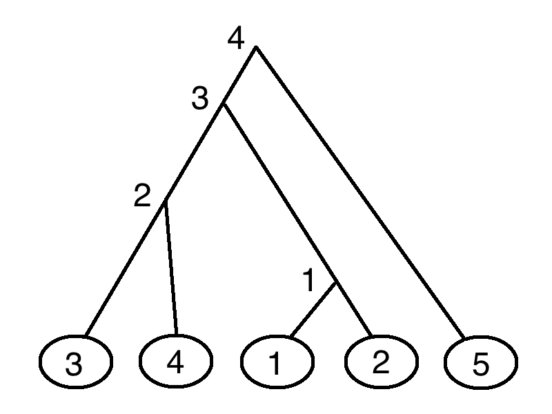
Example 2.3.

The maximal chain

\pi_{5}=1|2|3|4|5\lessdot 12|3|4|5\lessdot 12|34|5\lessdot 1234|5\lessdot 12345=\pi_{1}

in $\Pi_{5}$ corresponds to the ranked tree in Figure 1.

Proposition 2.4.

Let

C=\pi_{n}\lessdot\pi_{n-1}\lessdot\cdots\lessdot\pi_{1}

be a maximal chain in $\Pi_{n}$ , corresponding to a ranked phylogenetic tree. The cone of equidistant tree metrics compatible with $C$ is a simplicial cone whose extreme rays are the set of vectors $\{\delta_{\pi_{i}}:i=2,\ldots,n\}.$

This is a polyhedral geometry rewording of Theorem 7.2.8 of [18].

Example 2.5.

If an equidistant tree metric $d\in\mathbb{R}^{10}_{\geq 0}$ is compatible with the maximal chain in Example 2.3 then $d$ satisfies

d_{1,2}\leq d_{3,4}\leq d_{1,3}=d_{1,4}=d_{2,3}=d_{2,4}\leq d_{1,5}=d_{2,5}=d_{3,5}=d_{4,5}

and is in the simplicial cone with extreme rays

(1,1,1,1,1,1,1,1,1,1),(0,1,1,1,1,1,1,1,1,1),

(0,1,1,1,1,1,1,0,1,1),(0,0,0,1,0,0,1,0,1,1)

where the coordinates of $\mathbb{R}^{10}$ are labeled with the two-element sets $\{i,j\}\in{[5]\choose 2}$ in the lexicographic order.

Note that Proposition 2.4 also holds true when working with chains that are not maximal, which correspond to either trees with polytomies or situations where there are ties in the rankings of the internal vertices. These chains correspond to intersections of the maximal cones associated to the maximal chains in the partition lattice.

3. Geometry of Tree Space Near a Tritomy

The goal of this section to describe the geometry of tree space near a polytomy, in particular in the special case of tritomies. For rooted trees, a tritomy is an internal vertex that has three direct descendants. In an unrooted tree a tritomy is an internal vertex with four neighbors. When we speak of the “geometry of tree space near a tritomy”, we mean to describe the geometry of tree space near a generic tree metric that is the tree metric of a tree with a single tritomy and no other polytomies. The set of all such tritomy tree metrics, for a fixed topological structure on the tree $T$ , is a polyhedral cone of dimension one less than the dimension of tree space. Let $C_{T}$ denote this polyhedral cone. The tree $T$ with a single tritomy can be resolved to three binary trees. Denote them $T_{1},T_{2},T_{3}$ . The polyhedral cone of a tritomy $C_{T}$ is the intersection of the three resolution cones $C_{T_{1}}$ , $C_{T_{2}}$ , and $C_{T_{3}}$ associated to the three different ways to resolve the tritomy tree into a binary tree.

For both equidistant and ordinary tree space, the cones $C_{T}$ and their resolution cones $C_{T_{i}}$ , $i=1,2,3$ satisfy $\dim C_{T}=\dim C_{T_{i}}-1$ . This is easily seen by the simplicial structure of the cones $C_{T}$ for any tree $T$ , according to Propositions 2.2 and 2.4. Hence, locally near a generic point $x$ of $C_{T}$ , tree space looks like $\mathbb{R}^{k}\times K_{T}$ where $k=\dim C_{T}$ and $K_{T}$ is a one dimensional polyhedral fan that depends on $T$ but does not depend on $x$ . Furthermore, the fan $K_{T}$ can be chosen to live in a space orthogonal to the span of $C_{T}$ , and $\mathrm{span}\ K_{T}$ is two-dimensional. The goal of this section is to describe the structure of that fan $K_{T}$ . The analysis depends on the particular structure of the generators of the various cones involved, and the cases of equidistant tree metrics and arbitrary tree metrics must be handled separately. We treat these cases in Sections 3.1 and 3.2, respectively.

3.1. Equidistant Tree Space

In this section we determine the geometry of the fan $K_{T}$ for a tritomy tree $T$ in equidistant tree space. This tritomy tree has a node with three children. Denote the daughter clades of these children (that is, the set of leaves below each of children of the tritomy) by $A$ , $B$ , and $C$ . Let $T_{AB}$ , $T_{AC}$ , and $T_{BC}$ denote the three resolution trees, where for example $T_{AB}$ is the binary resolution where $A\cup B$ forms a clade. Note that since all the linear spaces that are involved are the same, instead of working with a fixed tree we can work with the corresponding rank function and chain in $\Pi_{n}$ to derive our results. This is what we will do in this section.

Let

K=\pi_{n}\lessdot\pi_{n-1}\lessdot\cdots\lessdot\pi_{k+1}\lessdot\pi_{k-1}\lessdot\cdots\lessdot\pi_{1}

be the chain corresponding to the polytomy tree. Note that this is a chain in the partition lattice which leaves out an element at the $k$ -th level. Here $\pi_{k+1}$ will contain among its blocks $A,B$ and $C$ , and $\pi_{k-1}$ will contain the block $A\cup B\cup C$ . The resolution trees $T_{AB}$ , $T_{AC}$ , and $T_{BC}$ correspond to the three ways to add a $\pi_{k}$ to this sequence which refines $\pi_{k+1}$ and is refined by $\pi_{k-1}$ .

We are interested in the linear spaces $\mathrm{span}\,C_{K}$ .

Lemma 3.1.

For any (not necessarily maximal) chain $K=\pi_{r}\lessdot\cdots\lessdot\pi_{1}$ , where $\pi_{1}=X$ , the set of vectors

\{\delta_{\pi_{i}}-\delta_{\pi_{i-1}}\}_{i=2,\ldots,r}

forms an orthogonal basis for $\mathrm{span}\ C_{K}$ .

Proof.

Since $\delta_{\pi_{2}},\ldots,\delta_{\pi_{r}}$ are the extreme rays of the simplicial cone $C_{K}$ , they are linearly independent and hence span $\mathrm{span}\ C_{K}$ . We can easily solve for the vectors $\delta_{\pi_{2}},\ldots,\delta_{\pi_{r}}$ given $\delta_{\pi_{i}}-\delta_{\pi_{i-1}},i=2,\ldots,r$ hence $\mathrm{span}\ C_{K}=\mathrm{span}\ \{\delta_{\pi_{i}}-\delta_{\pi_{i-1}}\}_{i=2,\ldots,r}$ . For all $i\in[r]$ , the positions of the ones in $\delta_{\pi_{i-1}}$ are a subset of the positions of the ones in $\delta_{\pi_{i}}$ . This guarantees that $\delta_{\pi_{i}}-\delta_{\pi_{i-1}}$ and $\delta_{\pi_{j}}-\delta_{\pi_{j-1}}$ do not have any nonzero entries in the same positions when $i\neq j$ . Hence these vectors are orthogonal. Note that $\delta_{\pi_{1}}$ is the zero vector if we assume that $\pi_{1}=X$ . ∎

The particular structure of the vectors $\delta_{\pi_{i+1}}-\delta_{\pi_{i}}$ will be useful in what follows.

Lemma 3.2.

Let $\pi$ and $\tau$ be two set partitions such that $\pi$ is a refinement of $\tau$ . Then

\delta_{\pi}-\delta_{\tau}=\sum e_{i,j}

where $i,j$ are in different parts of $\pi$ and the same part of $\tau$ .

Proof.

Trivial from the definition of $\delta_{\pi}$ . ∎

Now for each of the resolution cones, for example $C_{T_{AB}}$ , there is a unique ray $p_{AB}\in\mathrm{span}\,C_{T_{AB}}$ that is orthogonal to $\mathrm{span}\,C_{T}$ . We explain how to construct that ray now.

Lemma 3.3.

Let $a=|A|$ , $b=|B|$ , and $c=|C|$ . The vector $p_{AB}$ is given by

p_{AB}=-\frac{ac+bc}{ab+ac+bc}\delta_{A|B}+\frac{ab}{ab+ac+bc}(\delta_{A|C}+\delta_{B|C}).

Proof.

It suffices to start with any vector $r_{AB}\in\mathrm{span}\,C_{T_{AB}}\setminus\mathrm{span}\,C_{T}$ and project it onto the orthogonal complement of $\mathrm{span}\,C_{T}$ . We assume the tree $T$ is represented by the chain

K=\pi_{n}\lessdot\pi_{n-1}\lessdot\cdots\lessdot\pi_{k+1}\lessdot\pi_{k-1}\lessdot\cdots\lessdot\pi_{1}

and the tree $T_{AB}$ by the chain

K_{AB}=\pi_{n}\lessdot\pi_{n-1}\lessdot\cdots\lessdot\pi_{k+1}\lessdot\pi_{k}\lessdot\pi_{k-1}\lessdot\cdots\lessdot\pi_{1}.

For our vector we choose $r_{AB}=\delta_{\pi_{k}}-\delta_{\pi_{k-1}}$ . This vector is clearly not in $\mathrm{span}\,C_{K}$ since it involves $\delta_{\pi_{k}}$ . Furthermore, $r_{AB}$ is already orthogonal to all the vectors in the orthogonal basis for $\mathrm{span}\ C_{T}$ , except for the vector $\delta_{\pi_{k+1}}-\delta_{\pi_{k-1}}$ . Hence, we can project the vector $r_{AB}$ onto the complement of the space spanned by $\delta_{\pi_{k+1}}-\delta_{\pi_{k-1}}$ , this will be the same as projecting on the complement of $\mathrm{span}\ C_{T}$ .

Note that by Lemma 3.2 $r_{AB}=\delta_{A\cup B|C}=\delta_{A|C}+\delta_{B|C}$ . Similarly $\delta_{\pi_{k+1}}-\delta_{\pi_{k-1}}=\delta_{A|B|C}=\delta_{A|B}+\delta_{A|C}+\delta_{B|C}$ . So we want to project $\delta_{A|C}+\delta_{B|C}$ onto the orthogonal complement of $\delta_{A|B}+\delta_{A|C}+\delta_{B|C}$ . To find $p_{AB}$ it is enough to compute the component of $\delta_{A|C}+\delta_{B|C}$ that is perpendicular to $\delta_{A|B}+\delta_{B|C}+\delta_{A|C}$ , otherwise known as the vector rejection of $\delta_{B|C}+\delta_{A|C}$ from $\delta_{A|B}+\delta_{B|C}+\delta_{A|C}$ . Due to the orthogonality of the vectors $\delta_{A|B},\delta_{A|C}$ , and $\delta_{B|C}$ and the fact that, for example, $(||\delta_{A|B}||_{2})^{2}=|A||B|$ , we have

\frac{(\delta_{A|C}+\delta_{B|C})\cdot(\delta_{A|B}+\delta_{B|C}+\delta_{A|C})}{(\delta_{A|B}+\delta_{B|C}+\delta_{A|C})\cdot(\delta_{A|B}+\delta_{B|C}+\delta_{A|C})}=\frac{(||\delta_{B|C}||_{2})^{2}+(||\delta_{A|C}||_{2})^{2}}{(||\delta_{A|B}||_{2})^{2}+(||\delta_{B|C}||_{2})^{2}+(||\delta_{A|C}||_{2})^{2}}

So the vector rejection of $\delta_{B|C}+\delta_{A|C}$ from $\delta_{A|B}+\delta_{B|C}+\delta_{A|C}$ becomes

\delta_{A|C}+\delta_{B|C}-\frac{ac+bc}{ab+bc+ac}(\delta_{A|B}+\delta_{B|C}+\delta_{A|C})=

-\frac{ac+bc}{ab+ac+bc}\delta_{A|B}+\frac{ab}{ab+ac+bc}(\delta_{A|C}+\delta_{B|C}).

∎

This explicit formula for $p_{AB}$ implies that $\mathrm{span}\ K_{T}$ is 2-dimensional:

Corollary 3.4.

The space $\mathrm{span}\ K_{T}$ is 2-dimensional.

Proof.

The formulae for $p_{AB}$ , $p_{AC}$ and $p_{BC}$ given by Theorem 3.3 show that $p_{AB}$ and $p_{AC}$ are not parallel, so that $\mathrm{span}\ K_{T}$ is at least two-dimensional, but

p_{AB}+p_{AC}+p_{BC}=\mathbf{0},

where $\mathbf{0}$ denotes the zero vector in $\mathbb{R}^{n(n-1)/2}$ . So $\mathrm{span}\ K_{T}$ is exactly two dimensional. ∎

Corollary 3.4 also follows from the fact that the set of all equidistant tree metrics is a tropical variety in $\mathbb{R}^{n(n-1)/2}$ , as shown in [20].

Theorem 3.5.

The angle between the cones $C_{T_{AC}}$ and $C_{T_{BC}}$ is

\arccos\left(\frac{-c}{\sqrt{(a+c)(b+c)}}\right).

Proof.

We must calculate the angle between the vectors $p_{AC}$ and $p_{BC}$ . This is

\arccos\left(\frac{p_{AC}\cdot p_{BC}}{\|p_{AC}\|_{2}\|p_{BC}\|_{2}}\right).

Now

p_{AC}=-\frac{ab+bc}{ab+ac+bc}\delta_{A|C}+\frac{ac}{ab+ac+bc}(\delta_{A|B}+\delta_{B|C})

and

p_{BC}=-\frac{ab+ac}{ab+ac+bc}\delta_{B|C}+\frac{bc}{ab+ac+bc}(\delta_{A|B}+\delta_{A|C}).

Thus, $p_{AC}\cdot p_{BC}$ is given by

-\frac{ab+bc}{ab+ac+bc}\cdot\frac{bc}{ab+ac+bc}\cdot\|\delta_{A|C}\|_{2}^{2}+\frac{ac}{ab+ac+bc}\cdot\frac{bc}{ab+ac+bc}\cdot\|\delta_{A|B}\|_{2}^{2}-\frac{ac}{ab+ac+bc}\cdot\frac{ab+ac}{ab+ac+bc}\cdot\|\delta_{B|C}\|_{2}^{2}

\normalsize=\frac{-a^{2}bc}{ab+bc+ac}.

Similar calculations show that

\|p_{AC}\|_{2}=\sqrt{\frac{abc(a+c)}{ab+ac+bc}}\mbox{ and }\|p_{BC}\|_{2}=\sqrt{\frac{abc(b+c)}{ab+ac+bc}}.

Combining these pieces produces the formula in the Theorem. ∎

3.2. Tree Space

In this section we determine the geometry of the fan $K_{T}$ for a tritomy tree $T$ in unrooted tree space $\mathcal{T}_{n}$ . The approach is similar to the analysis for equidistant tree space, but the structure of tree space is more complicated. In particular, finding an orthogonal basis for the space spanned by the rays of the intersection cone for a tritomy is less straightforward.

Recall that a tritomy $p$ in an unrooted tree is an internal vertex of degree four. The edges adjacent to $p$ induce a four-way set partition $A|B|C|D$ of $[n]$ . Let $T_{AB}$ denote the resolution tree in which there is an edge inducing the split $A\cup B|C\cup D$ . Note that $T_{AB}=T_{CD}$ . So there are three resolutions $T_{AB},T_{AC}$ and $T_{AD}$ of $T$ . For the remainder of this section, let $a=|A|$ , $b=|B|$ , $c=|C|$ , and $d=|D|$ . Let $r_{AB}=\delta_{A\cup B|C\cup D}$ .

Lemma 3.6.

Let $T$ be an unrooted tree with a tritomy and corresponding partition $A|B|C|D$ of $[n]$ . Then $r_{AB}\in\mathrm{span}\ C_{T_{AB}}\setminus\mathrm{span}\ C_{T}$ , and $\dim\mathrm{span}\ C_{T}=2n-4$ .

Proof.

By Proposition 2.2 each extreme ray of $C_{T_{AB}}$ (equivalently, $T$ ) comes from a split induced by an edge of $T_{AB}$ (equivalently, an edge of $T$ ). A binary unrooted tree on $n$ leaves has $2n-3$ edges. So the cone $C_{T_{AB}}$ has $2n-3$ rays, one for each internal edge of the tree $T_{AB}$ . By contracting the edge that induces the split $A\cup B|C\cup D$ for any pair we obtain $T$ . Therefore $C_{T}$ has $2n-4$ extreme rays that correspond to the $2n-4$ internal edges of $T$ . Since $C_{T}$ is simplicial, $\dim\mathrm{span}\ C_{T}=2n-4$ . ∎

The projections $p_{AB}$ , $p_{AC}$ and $p_{AD}$ of $r_{AB}$ , $r_{AC}$ and $r_{AD}$ onto $(\mathrm{span}\ C_{T})^{\perp}$ are the maximal cones in the fan $K_{T}$ . As in the previous section, we use an orthogonal basis of $\mathrm{span}\ C_{T}$ to simplify the necessary calculations.

The vectors in the set $\mathcal{U}=\{\delta_{A|B\cup C\cup D},\delta_{B|A\cup C\cup D},\delta_{C|A\cup B\cup D},\delta_{D|A\cup B\cup C}\}$ are extreme rays of $T$ . The elements of $\mathcal{U}$ correspond to the four edges in $T$ adjacent to the tritomy $p$ . We show in the next Lemma that to calculate $p_{AB}$ it is sufficient to calculate the projection of $r_{AB}$ onto $(\mathrm{span}\ \mathcal{U})^{\perp}$ . First we require some additional notation: let $e=(u,v)$ be an edge of $T$ not adjacent to $p$ where $v$ is the internal vertex of $T$ on the path to $p$ from $e$ . Let $e^{\prime}=(w,v)$ be the unique edge in $T$ satisfying the conditions $(i)$ $e\neq e^{\prime}$ and $(ii)$ $w$ appears on the path from $v$ to $p$ in $T$ (note that it is possible that $w=p$ ). Let $A_{e}|B_{e}$ be the split of $[n]$ induced by $e$ and let $A_{e^{\prime}}|B_{e^{\prime}}$ be the split of $[n]$ induced by $e^{\prime}$ . Note $A_{e}\subsetneq A_{e^{\prime}}$ . Let $a_{e}=|A_{e}|$ and $a_{e^{\prime}}=|A_{e^{\prime}}|$ . Let

\mathcal{V}=\left\{\delta_{A_{e}|B_{e}}-\frac{a_{e}}{a_{e^{\prime}}}\delta_{A_{e^{\prime}}|B_{e^{\prime}}}\ :\ p\notin e=(u,v),\ e^{\prime}\ \text{satisfies}\ (i),(ii)\right\}.

Lemma 3.7.

Every vector in $\mathcal{V}$ is orthogonal to $r_{AB},r_{AC}$ and $r_{AD}$ and $\mathcal{U}\cup\mathcal{V}$ is a basis for $\mathrm{span}\ C_{T}$ .

Proof.

Since $T$ has exactly one tritomy, $T$ has $2n-4$ edges. When $n=4$ , $2n-4=4$ . In this case $|\mathcal{U}|=\dim\mathrm{span}\ C_{T}$ , and $\mathcal{U}$ is a basis for $\mathrm{span}\ C_{T}$ . So, assume $n>4$ , then $\mathcal{V}$ is not empty because we can find edges $e$ and $e^{\prime}$ satisfying $p\notin(u,v)=e$ and $e^{\prime}$ satisfying conditions $(i)$ and $(ii)$ . We will first show that each element of $\mathcal{V}$ is orthogonal to $r_{AB},r_{AC}$ , and $r_{AD}$ . Let $\nu\in\mathcal{V}$ , then

\nu=\delta_{A_{e}|B_{e}}-\frac{a_{e}}{a_{e^{\prime}}}\delta_{A_{e^{\prime}}|B_{e^{\prime}}}

Note that $A_{e^{\prime}}$ is contained in one of $A,B,C$ , and $D$ . Without loss of generality we may assume that $A_{e^{\prime}}\subset A$ . Then it follows directly from the structure of the summands in the vector $\nu$ that

r_{AB}\cdot\nu=(a_{e^{\prime}})(c+d)\left(-\frac{a_{e}}{a_{e^{\prime}}}\right)+a_{e}(c+d)=0

Similar calculations show that $r_{AC}$ and $r_{AD}$ are also orthogonal to $\nu$ .

We obtain $2n-8$ vectors in $\mathcal{V}$ because there are $(2n-4)-4$ edges in $T$ that do not induce vectors in $\mathcal{U}$ . So $|\mathcal{U}\cup\mathcal{V}|=2n-4$ . Since $\mathcal{U}\cup\mathcal{V}$ is comprised of vectors that are linear combinations of split-pseudometrics, $\mathrm{span}\ \mathcal{U}\cup\mathcal{V}\subset\mathrm{span}\ C_{T}$ . The set $\mathcal{U}\cup\mathcal{V}$ is also linearly independent since it can be seen as an upper triangular transformation of the set of extreme rays of $C_{T}$ , which were independent. Thus $\mathcal{U}\cup\mathcal{V}$ is a basis for $\mathrm{span}\ C_{T}$ . ∎

Due to the structure of the vectors $r_{AB}$ and the elements of $\mathcal{U}$ , $p_{AB}$ is constant on the coordinates for each $\delta_{U|V}$ and we can write

(1)

p_{AB}=\sum_{\{U,V\}\in{\{A,B,C,D\}\choose 2}}w(AB)_{U|V}\cdot\delta_{U|V}

the coefficients $w(AB)_{U|V}$ will facilitate computation of dot products and 2-norms.

Theorem 3.8.

The angle between the cones $C_{T_{AB}}$ and $C_{T_{AC}}$ is

\arccos\left(-\frac{bc+ad}{\sqrt{(a+b)(a+c)(b+d)(c+d)}}\right)

Proof.

By Lemma 3.7, to find $p_{AB}$ , $p_{AC}$ , and $p_{AD}$ it is sufficient to calculate the projection of $r_{AB}$ , $r_{AC}$ , and $r_{AD}$ onto $(\mathrm{span}\ \mathcal{U})^{\perp}$ . We will find $p_{AB}$ by calculating the coefficients $w(AB)_{U|V}$ . First, we construct a matrix $M_{AB}$ where $(M_{AB})_{i,j}$ is obtained (up to row operations) by taking the dot product of the vector indexing row $i$ and column $j$ :

M_{AB}=\begin{matrix}[c|ccccc]\quad&r_{AB}&\delta_{A|B\cup C\cup D}&\delta_{B|A\cup C\cup D}&\delta_{C|A\cup B\cup D}&\delta_{D|A\cup B\cup C}\\ \hline\cr\delta_{A|B\cup C\cup D}&c+d&b+c+d&b&c&d\\ \delta_{B|A\cup C\cup D}&c+d&a&a+c+d&c&d\\ \delta_{C|A\cup B\cup D}&a+b&a&b&a+b+d&d\\ \delta_{D|A\cup B\cup C}&a+b&a&b&c&a+b+c\end{matrix}

Next, let $K_{AB}$ be the matrix given below:

K_{AB}=\begin{matrix}[c|ccccc]\quad&r_{AB}&\delta_{A|B\cup C\cup D}&\delta_{B|A\cup C\cup D}&\delta_{C|A\cup B\cup D}&\delta_{D|A\cup B\cup C}\\ \hline\cr\delta_{A|B}&0&1&1&0&0\\ \delta_{A|C}&1&1&0&1&0\\ \delta_{A|D}&1&1&0&0&1\\ \delta_{B|C}&1&0&1&1&0\\ \delta_{B|D}&1&0&1&0&1\\ \delta_{C|D}&0&0&0&1&1\end{matrix}

Let $\sigma_{AB}=\sigma_{1}r_{AB}+\sigma_{2}\delta_{A|B\cup C\cup D}+\sigma_{3}\delta_{B|A\cup C\cup D}+\sigma_{4}\delta_{C|A\cup B\cup D}+\sigma_{5}\delta_{D|A\cup B\cup C}$ be a vector in the null space of the matrix $M_{AB}$ . Up to a scalar multiple,

K_{AB}(\sigma_{AB})=\left[\begin{matrix}w(AB)_{A|B}\\ w(AB)_{A|C}\\ w(AB)_{A|D}\\ w(AB)_{B|C}\\ w(AB)_{B|D}\\ w(AB)_{C|D}\end{matrix}\right]=\left[\begin{matrix}(a+b)cd(c+d)\\ -bd(bc+ad)\\ -bc(ac+bd)\\ -ad(ac+bd)\\ -ac(bc+ad)\\ ab(a+b)(c+d)\end{matrix}\right]

Then

(2)

p_{AB}\cdot p_{AC}=\sum_{\{U,V\}\in{\{A,B,C,D\}\choose 2}}|U|\cdot|V|\cdot w(AB)_{U|V}\cdot w(AC)_{U|V}

and

(3)

||p_{AB}||_{2}=\sqrt{\sum_{\{U,V\}\in{\{A,B,C,D\}\choose 2}}|U|\cdot|V|\cdot[w(AB)_{U|V}]^{2}}.

We use (2) and (3) to obtain the formulae for the angle measures between the resolution cones. ∎

Corollary 3.9.

The space $\mathrm{span}\ K_{T}$ is 2-dimensional when $T$ is unrooted.

Proof.

As in the case of rooted trees, we can use the formula in (1) to show that the set $\{p_{AB},p_{AC}\}$ is linearly independent, but the set $\{p_{AB},p_{AC},p_{BC}\}$ is linearly dependent. ∎

Corollary 3.9 also follows from the fact that the set of all arbitrary tree metrics is a tropical variety in $\mathbb{R}^{n(n-1)/2}$ , as shown in [20].

4. Distance-Based Methods Near a Tritomy

In this section, we analyze the performance of distance-based methods around a tritomy using the results on the geometry of tree space from Section 3. The basic observation is this: any phylogenetic algorithm decomposes the set of all dissimilarity maps into regions based upon which combinatorial type of tree gets reconstructed by the algorithm. While in many cases we do not have a complete understanding of the geometry of these decompositions across all of $\mathbb{R}^{n(n-1)/2}_{\geq 0}$ , we can describe the geometry in a small neighborhood of a tree metric with a single tritomy. It is this geometry which we explore in the present section.

4.1. Least Squares Phylogeny

Let $C_{1},\ldots,C_{r}$ be subsets of $\mathbb{R}^{n(n-1)/2}$ . The Voronoi cell $V_{k}$ associated with the subset $C_{k}$ is the set of all points

V_{k}=\{\mathbf{x}\in\mathbb{R}^{n(n-1)/2}\ |\ d(\mathbf{x},C_{k})\leq d(\mathbf{x},C_{j})\ \text{for \ all }j\neq k\}

where $d(\mathbf{x},C_{k})=\inf\{||\mathbf{x}-\mathbf{a}||_{2}\ |\ \mathbf{a}\in C_{k}\}$ . The Voronoi decomposition is the subdivision of $\mathbb{R}^{n(n-1)/2}$ into Voronoi cells of the set $\{C_{k}\}$ . When $\{C_{k}\}$ is the collection of cones associated to all possible combinatorial trees with leaf set $[n]$ , the Voronoi cells comprise the subdivision of space induced by the least squares phylogeny problem.

While the Voronoi decomposition of a finite set of points is well-known to be a polyhedral subdivision of space, the Voronoi decomposition induced by a collection of higher dimensional polyhedra can be a complicated semi-algebraic decomposition. Hence, the Voronoi decomposition induced by the tree cones is probably not polyhedral. We saw in Section 3 that in a neighborhood of a tree metric $T$ with a single tritomy, tree space has the form $\mathbb{R}^{k}\times K_{T}$ , where $k=\dim\ \mathrm{span}\ C_{T}$ and $K_{T}$ is a one-dimensional fan with three rays that sits naturally inside a two dimensional linear space $\mathrm{span}\ K_{T}$ . In this setting it is easy to describe the Voronoi decomposition.

Proposition 4.1.

Let $T$ be a tree metric in $\mathbb{R}^{n(n-1)/2}_{\geq 0}$ with local tree space $\mathbb{R}^{k}\times K_{T}$ . The boundary between the Voronoi cells for the resolution cones $C_{T_{AB}}$ and $C_{T_{AC}}$ are completely determined by the angle bisector in $\mathrm{span}\ K_{T}$ between $p_{AB}$ and $p_{AC}$ .

Proof.

The Euclidean distance between the cones $C_{T_{AB}}$ and $C_{T_{AC}}$ is the sum of the distance between them in the two orthogonal spaces $\mathrm{span}\ C_{T}$ and $\mathrm{span}\ K_{T}$ . Of these two distances, only the distance in the two-dimensional space $\mathrm{span}\ K_{T}$ is nonzero; this distance is determined by the angle between the maximal cones in the 1-dimensional polyhedral fan $K_{T}$ . The set of all points in the plane $\mathrm{span}\ K_{T}$ equidistant between two vectors emanating from the origin is the bisector of the angle between the two vectors. ∎

Proposition 4.1 allows us to easily compute the relative size of the Voronoi regions around a polytomy for either equidistant or ordinary tree metrics. The next theorem gives a formula for the boundary between the Voronoi regions.

Theorem 4.2.

Let $T$ be a ranked, rooted tree with a single tritomy. The boundary of the Voronoi cell in $\mathrm{span}\ K_{T}$ between the resolution cones $C_{T_{AB}}$ and $C_{T_{AC}}$ is spanned by the vector

\frac{p_{AB}}{\sqrt{a+b}}+\frac{p_{AC}}{\sqrt{a+c}}.

Proof.

By Proposition 4.1 the boundary of the cell we wish to compute is given by by the angle bisector in $\mathrm{span}\ K_{T}$ between $p_{AB}$ and $p_{AC}$ , which is spanned by the normalized average of the two vectors. By Lemma 3.3 we have

\|p_{AB}\|_{2}=\sqrt{\frac{abc(a+b)}{ab+ac+bc}}\mbox{ and }\|p_{AC}\|_{2}=\sqrt{\frac{abc(a+c)}{ab+ac+bc}}

Therefore

\frac{p_{AB}}{\|p_{AB}\|}+\frac{p_{AC}}{\|p_{AC}\|}=\sqrt{\frac{ab+ac+bc}{abc}}\left(\frac{p_{AB}}{\sqrt{a+b}}+\frac{p_{AC}}{\sqrt{a+c}}\right)

So $\frac{p_{AB}}{\sqrt{a+b}}+\frac{p_{AC}}{\sqrt{a+c}}$ spans the boundary of the Voronoi cells for the two cones in $\mathrm{span}\ K_{T}$ . ∎

Theorem 4.3.

Let $T$ be an unrooted tree with a single tritomy. The boundary of the Voronoi cell in $\mathrm{span}\ K_{T}$ between the resolution cones $C_{T_{AB}}$ and $C_{T_{AC}}$ is spanned by the vector

\frac{p_{AB}}{\sqrt{(a+b)(c+d)}}+\frac{p_{AC}}{\sqrt{(a+c)(b+d)}}.

Proof.

We use the fact that $p_{AB}$ and $p_{AC}$ are constant on the vectors $\delta_{U|V}$ for $\{U,V\}\in{\{A,B,C,D\}\choose 2}$ and the formulas for the coeffcients $w(A,B)_{U|V}$ in the proof of Theorem 3.8 to calculate the 2-norms of $p_{AB}$ and $p_{AC}$ . Up to an identical polynomial $f$ in the variables $a,b,c$ and $d$ , we have

(4)

\|p_{AB}\|_{2}=f\cdot\sqrt{(a+b)(c+d)}

and

(5)

\|p_{AC}\|_{2}=f\cdot\sqrt{(a+c)(b+d)}

As in Theorem 4.2 we know that the angle bisector between $p_{AB}$ and $p_{AC}$ gives the boundary of the Voronoi cell in $\mathrm{span}\ K_{T}$ . By (4) and (5) the angle bisector is a multiple of

\frac{p_{AB}}{\sqrt{(a+b)(c+d)}}+\frac{p_{AC}}{\sqrt{(a+c)(b+d)}}.

∎

4.2. UPGMA Regions Near a Polytomy

The UPGMA algorithm (Unweighted Pair Group Method with Arithmetic Mean) [19] is an agglomerative tree reconstruction method that takes as an input $\alpha$ , a dissimilarity map of ${n\choose 2}=n(n-1)/2$ pairwise distances between a set $X$ of $n$ taxa, and returns a rooted equidistant tree metric $d$ on $X$ . The metric $d$ is an approximation to the least squares phylogeny for $\alpha$ . In this section we show that in some circumstances, UPGMA fails to correctly identify the least squares phylogeny. The occurrence and severity of this failure depends entirely on the relative sizes of the daughter clades $A$ , $B$ , and $C$ of the tritomy. The algorithm works as follows:

Algorithm 4.1 UPGMA

•

Input: a dissimilarity map $\alpha\in\mathbb{R}^{{n(n-1)/2}}_{\geq 0}$ on $[n]$ .
•

Output: a maximal chain $C$ in the partition lattice $\Pi_{n}$ and an equidistant tree metric $d$ .
•

Initialize $\pi_{n}=1|2|\cdots|n$ , and set $\alpha^{n}=\alpha$ .

•

For $i=n-1,\ldots,1$ do

–

From partition $\pi_{i+1}=\lambda^{i+1}_{1}|\cdots|\lambda^{i+1}_{i+1}$ and distance vector $\alpha^{i+1}\in\mathbb{R}^{(i+1)i/2}_{\geq 0}$ choose $j,k$ be so that $\alpha^{i+1}(\lambda^{i+1}_{j},\lambda^{i+1}_{k})$ is minimized.
–

Set $\pi_{i}$ to be the partition obtained from $\pi_{i+1}$ by merging $\lambda^{i+1}_{j}$ and $\lambda^{i+1}_{k}$ and leaving all other parts the same. Let $\lambda^{i}_{i}=\lambda^{i+1}_{j}\cup\lambda^{i+1}_{k}$ .

–

Create new distance $\alpha^{i}\in\mathbb{R}^{i(i-1)/2}_{\geq 0}$ by $\alpha^{i}(\lambda,\lambda^{\prime})=\alpha^{i+1}(\lambda,\lambda^{\prime})$ if $\lambda,\lambda^{\prime}$ are both parts of $\pi_{i+1}$ and

\alpha^{i}(\lambda,\lambda^{i}_{i})=\frac{|\lambda^{i+1}_{j}|}{|\lambda^{i}_{i}|}\alpha^{i+1}(\lambda,\lambda^{i+1}_{j})+\frac{|\lambda^{i+1}_{k}|}{|\lambda^{i}_{i}|}\alpha^{i+1}(\lambda,\lambda^{i+1}_{k})

otherwise.

–

For each $x\in\lambda^{i+1}_{j}$ and $y\in\lambda^{i+1}_{k}$ , set $d(x,y)=\alpha^{i+1}(\lambda^{i+1}_{j},\lambda^{i+1}_{k})$ .

•

Return: Chain $C=\pi_{n}\lessdot\cdots\lessdot\pi_{1}$ and equidistant metric $d$ .

Note that if the blocks $A,B\subset[n]$ are joined in step $i$ of Algorithm 4.1 the distance recalculation implies

\alpha^{i}(A,B)=\frac{1}{|A||B|}\sum_{x\in A,y\in B}\alpha^{n}(x,y)=\frac{1}{ab}\sum_{x\in A,y\in B}\alpha(x,y),

a formula which is useful in the next Proposition:

Proposition 4.4.

Let $T$ be a ranked, rooted tree with a single tritomy. The boundaries between UPGMA regions in $\mathbb{R}^{n(n-1)/2}_{\geq 0}$ for the resolution cones $C_{T_{AB}}$ , $C_{T_{AC}}$ and $C_{T_{BC}}$ are orthogonal to the plane $\mathrm{span}\ K_{T}$ .

Proof.

The boundary between the UPGMA regions for the cones $C_{T_{AC}}$ and $C_{T_{BC}}$ is given by the condition

\alpha^{k}(A,C)=\alpha^{k}(B,C)

which translates into the following linear condition on the original dissimilarity map

\frac{1}{ac}\sum_{i\in A,j\in C}\alpha(i,j)=\frac{1}{bc}\sum_{i\in B,j\in C}\alpha(i,j).

This hyperplane has normal vector

\frac{1}{ac}\delta_{A|C}-\frac{1}{bc}\delta_{B|C}.

Now

-\frac{1}{ac}p_{AC}=\frac{1}{ab+ac+bc}\left(-\delta_{A|B}-\delta_{B|C}+\frac{ab+bc}{ac}\delta_{A|C}\right)

and

\frac{1}{bc}p_{BC}=\frac{1}{ab+ac+bc}\left(\delta_{A|B}+\delta_{A|C}-\frac{ab+ac}{bc}\delta_{B|C}\right)

-\frac{1}{ac}p_{AC}+\frac{1}{bc}p_{BC}=\frac{1}{ab+ac+bc}\left(\left(\frac{ab+bc}{ac}+1\right)\delta_{A|C}-\left(\frac{ab+ac}{bc}+1\right)\delta_{B|C}\right)

=\frac{1}{ac}\delta_{A|C}-\frac{1}{bc}\delta_{B|C}.

Thus, the normal vector for the boundary between UPGMA regions for the cones $C_{T_{AC}}$ and $C_{T_{BC}}$ is in $\mathrm{span}\ K_{T}$ , and the boundary is orthogonal to $\mathrm{span}\ K_{T}$ . The calculation is the same for the other two pairs of cones. ∎

Theorem 4.5.

The boundary between the UPGMA cells for the resolution tree topologies $T_{AC}$ and $T_{BC}$ in $\mathrm{span}\ K_{T}$ is $-p_{AB}$ .

Proof.

Since $\mathrm{span}\ K_{T}$ is two-dimensional and the boundaries between the UPGMA regions for the resolutions $T_{AB}$ , $T_{AC}$ and $T_{BC}$ are orthogonal to $K_{T}$ by Proposition 4.4, it suffices to find a vector $\omega\in\mathrm{span}\ K_{T}$ that satisfies

\frac{1}{ac}\sum_{i\in A,j\in C}\omega_{i,j}=\frac{1}{bc}\sum_{k\in B,\ell\in C}\omega_{k,\ell}\leq\frac{1}{ab}\sum_{m\in A,n\in B}\omega_{m,n}.

Any such vector will span the boundary of the UPGMA cells. We have

\frac{1}{ac}\sum_{i\in A,j\in C}-(p_{AB})_{i,j}=\frac{1}{bc}\sum_{k\in B,\ell\in C}-(p_{AB})_{k,\ell}=-\frac{ab}{ab+ac+bc}

while

\frac{1}{ab}\sum_{m\in A,n\in B}-(p_{AB})_{m,n}=\frac{ac+bc}{ab+ac+bc}

So $-p_{AB}$ satisfies the required condition. ∎

4.3. UPGMA and LSP Cells

In this section we discuss how results from Sections 3 and 4 show that UPGMA poorly matches LSP in some circumstances. The geometry of the fan $K_{T}$ and the UPGMA cells in $\mathrm{span}\ K_{T}$ for equidistant trees depends entirely on the size of the daughter clades $A,B$ , and $C$ of the tritomy. Consequentially, the quality of the performance of UPGMA near a tree metric with a tritomy depends on how similar in size the daughter clades are. When $a=b=c$ , the UPGMA and LSP regions near a tritomy are the same, but as either one or two of the daughter clades becomes much larger, UPGMA does a poorer job of identifying the LSP. We also use results from Section 4 to show that NJ poorly matches LSP in specific examples for small numbers of taxa.

We can use our theorems about the geometry of $\mathrm{span}\ K_{T}$ to investigate the relative size of the UPGMA and Voronoi cells as $a,b$ , and $c$ vary. By Theorem 3.5 the angle between $C_{T_{AC}}$ and $C_{T_{BC}}$ is

\arccos\left(\frac{-c}{\sqrt{(a+c)(b+c)}}\right)

and this is also the angle measure of the UPGMA region associated with the cone $C_{T_{AB}}$ . By the angle bisector argument, we see that the angle measure of the LSP region associated to the tree $T_{AB}$ near the tritomy will be:

\frac{1}{2}\arccos\left(\frac{-a}{\sqrt{(a+b)(a+c)}}\right)+\frac{1}{2}\arccos\left(\frac{-b}{\sqrt{(a+b)(b+c)}}\right).

When $c>>a\approx b$ , the angle for the UPGMA region approaches $\pi$ whereas the angle for the LSP region approaches $\pi/{2}$ . Conversely, when $a\approx b>>c$ the angle for the UPGMA region approaches $\pi/2$ whereas the angle for the LSP region approaches $3\pi/4$ . Tables 1 and 2 compare the sizes of the various regions for differing values of $a,b,$ and $c$ . We display the sizes as the percentage of the total amount of the local volume around the polytomy that corresponds to the UPGMA or LSP region for the cone $C_{T_{AB}}$ .

Table 1. Region sizes for

C_{T_{AB}}

when

c>>a=b

a	b	c	UPGMA	LSP
1	1	1	33.3333	33.3333
1	1	2	36.6139	31.693
1	1	4	39.7583	30.1209
1	1	8	42.4261	28.787
1	1	16	44.5139	27.7431
1	1	$2^{10}$	49.297	25.3515
1	1	$2^{20}$	49.978	25.011

Table 2. Region sizes for

C_{T_{AB}}

when

a=b>>c

a	b	c	UPGMA	LSP
1	1	1	33.3333	33.3333
2	2	1	30.4086	34.7957
4	4	1	28.2046	35.8977
8	8	1	26.7721	36.6139
16	16	1	25.9367	37.0317
$2^{10}$	$2^{10}$	1	25.0155	37.4923
$2^{20}$	$2^{20}$	1	25.0001	37.4999

While the convergence to the limiting values is slow, already for small values of $a,b$ , and $c$ there is significant discrepancy between UPGMA and LSP. Figures 5 and 6 illustrate the geometry of this phenomenon for the two extreme cases $c>>a\approx b$ , and $a\approx b>>c$ . In both figures the fan $K_{T}$ is black, the vector $p_{AB}$ is labeled with the pair $AB$ , LSP boundaries are blue, and UPGMA boundaries are red. Note that when $c>>a\approx b$ , UPGMA overestimates the size of the LSP region for $C_{T_{AB}}$ . When $a\approx b>>c$ , UPGMA underestimates the size of the LSP region for $C_{T_{AB}}$ .

LSP Cells and Local NJ Behavior

The Neighbor-Joining (NJ) algorithm, due to Saitou and Nei [17] is a distance-based reconstruction method that returns an unrooted tree $T$ and a tree metric realized by $T$ . Both the selection criterion (known as the ” $Q$ -criterion”) and distance recalculation are linear combinations of the original input coordinates. Therefore, as in the case of UPGMA, NJ divides the input space $\mathbb{R}^{n(n-1)/2}_{\geq 0}$ into a family of polyhedral cones studied in [10] and [15].

A complete combinatorial description of the NJ cones remains unknown, and we do not have a closed description of the local geometry of the NJ regions around a tritomy. However, by running NJ on points sampled uniformly from the surface of a small sphere around a tritomy, we can obtain an empirical estimate of the local relative size of NJ regions for small numbers of taxa.

For unrooted tree metrics, the case of interest is when $a$ and $b$ are larger than $c$ and $d$ : if $a=b=c$ and $d$ is larger or smaller, the size of the LSP cells the for three resolution cones will be symmetric. NJ poorly identifies LSP when $a$ and $b$ are larger than $c$ and $d$ even for small numbers of taxa. Unlike in the case of UPGMA, the relative size of the regions appears to be dictated not only by $a,b,c$ , and $d$ , but also by the topology of the subtrees with leaf sets $A,B,C$ , and $D$ .

Algorithm 4.2 Neighbor-Joining

•

Input: a dissimilarity map $\alpha\in\mathbb{R}^{{n(n-1)/2}}_{\geq 0}$ on $[n]$ .
•

Output: an unrooted binary tree $T$ and a tree metric $d_{T,w}=d$ realized by $T$ .
•

Initialize $[n]=\{1,2,...,n\}$ , and set $d_{0}=\alpha$ .

•

For $r=1,\ldots,n-3$ do

–

Identify subsets $A_{i},A_{j}$ of $[n]$ minimizing

Q_{r}(A_{i},A_{j})=(n-r-1)d_{r-1}(A_{i},A_{j})-\sum_{k=1}^{n-r+1}d_{r}(A_{i},A_{k})-\sum_{k=1}^{n-r+1}d_{r}(A_{j},A_{k})

–

Update

$d_{r}(A_{ij},A_{k})=\frac{1}{2}\left(d_{r-1}(A_{i},A_{k})+d_{r-1}(A_{j},A_{k})-d_{r}(A_{i},A_{j})\right)$

•

Return: unrooted binary combinatorial tree $T$ , $w:E(T)\rightarrow\mathbb{R}$ and tree metric $d_{n-3}=d_{T,w}$ .

Applying Theorem 3.8, we see that when $a\approx b>>c\approx d$ , the angle between the cones $C_{T_{AC}}$ and $C_{T_{AD}}$ approaches $\pi$ , while the LSP angle for $C_{T_{AB}}$ , bounded by angle bisectors between the two pairs $\{p_{AB},p_{AC}\}$ and $\{p_{AB},p_{AD}\}$ , approaches $\pi/2$ . Figure 7 shows this case. The fan $K_{T}$ is black, and the LSP boundaries are blue.

For small values of $a,b,c$ and $d$ we present computational evidence that NJ fails to identify LSP correctly. Consider the tree metrics $d_{1}$ and $d_{2}$ with topologies shown in Figures 8 and 9 and given edge weights of randomly assigned numbers between 5000 and 10000. Here $A=\{1,2,3,4,5,6\},B=\{7,8,9,10,11,12\},C=\{13\}$ , and $D=\{14\}$ . Using Theorem 3.8 we can calculate the angles between the pairs of cones in $\{C_{T_{AB}},C_{T_{AC}},C_{T_{AD}}\}$ and find the relative sizes of the LSP regions near the tritomies $d_{1}$ and $d_{2}$ . Recall that one consequence of Theorem 3.8 is that the relative size of the LSP regions near $d_{1}$ and $d_{2}$ will be the same because these proportions only depend on $a,b,c$ , and $d$ .

Running NJ on 1,000,000 points sampled uniformly from spheres of radius 0.05 centered at $d_{1}$ and $d_{2}$ gives an empirical measure of the size of NJ regions for the three resolutions $T_{AB}$ , $T_{AC}$ and $T_{AD}$ near the two points. We compare this empirical distribution with the size of the LSP regions computed via Theorem 3.7 in Table 3. Sizes of the regions are given as percentages of the total local volume near the tritomy.

Table 3. NJ and LSP near

d_{1}

and

d_{2}

Resolution of Splits	LSP	NJ : $d_{1}$	NJ: $d_{2}$
$AB\|CD$	30.6897	38.1501	35.7037
$AC\|BD$	34.6552	30.9344	32.1305
$AD\|BC$	34.6552	30.9155	32.1658

Table 3 shows that NJ overestimates the size of the LSP regions near $d_{1}$ and $d_{2}$ closest to the cone $C_{T_{AB}}$ and underestimates the regions near $C_{T_{AC}}$ and $C_{T_{AD}}$ . Furthermore, the topological structure of the subclades $A$ and $B$ influence the local size of the NJ regions. This shows that a direct analog of Theorem 4.5 will not exist for NJ. However, there may exist an analogous theorem for NJ when the topology of the subtrees around the polytomy is taken into account.

5. Conclusion

Distance-based heuristics like UPGMA and NJ can be seen as approximating solutions to the intuitively appealing but NP-hard least-squares phylogeny problem. We compared heuristics to LSP when the true tree metric contains a tritomy. For UPGMA, our theoretical analysis shows that the success rate of the heuristic greatly depends on how balanced the sizes of the underlying daughter clades are.

Due to the precise form of input data used by NJ and the outputs of the algorithm, NJ is an approximation to LSP. However, Gascuel and Steel showed that NJ performs a heuristic search, guided by the $Q$ -criterion at each agglomeration step, that minimizes a tree-length estimate due to Pauplin known as the ”Balanced Minimum Evolution” (BME) criterion ([16], [14]). This insight was incorporated into the selection criterion and distance recalculation aspects of the algorithms BIONJ [13], Weighbor [6], and FastME [9]. These algorithms take distance matrices as input and have superior performance to NJ in terms of topological accuracy and better immunity to pathologies such as the long-branch attraction. However, the subdivision of the input spaces induced by each of these improved algorithms is not polyhedral and, like the Voronoi cells around higher-degree polytomies, have a complicated semi-algebraic description.

Any improvements to distance-based methods implied by the results in this paper would require a fundamentally different approach, such as changing the $Q$ -criterion at each step to reflect the size of the taxon groups to be joined.

Acknowledgments

Ruth Davidson was partially supported by the US National Science Foundation (DMS 0954865). Seth Sullivant was partially supported by the David and Lucille Packard Foundation and the US National Science Foundation (DMS 0954865).

References

[1] F. Ardila and C. J. Klivans. The Bergman complex of a matroid and phylogenetic trees. Journal of Combinatorial Theory, Series B 96 (2006): 38-49.
[2] K. Atteson. The performance of the NJ method of phylogeny reconstruction. In: Mathematical Hierarchies and Biology, DIMACS Series in Discrete Mathematics and Theoretical Computer Science 37 (eds. Mirkin et al.) AMS, Providence, RI, (1997) 133–147
[3] L.J. Billera, S. Holmes, and K. Vogtmann. Geometry of the space of phylogenetic trees, Advances in Applied Mathematics 27 (2001) 733-767.
[4] P. Buneman. A note on metric properties of trees, Journal of Combinatorial Theory, Series B 17 (1974) 48-50.
[5] P. Buneman. The recovery of trees from measures of dissimilarity. In Mathematics and the Archeological and Historical Sciences. Edinburgh University Press, 387-395.
[6] W.M. Bruno, N.D. Socci, and A.L. Halpern. Weighted Neighbor Joining: a likelihood-based approach to distance- based phylogeny reconstruction. Molecular Biology and Evolution 17 (2000):189Ð 197.
[7] R. Davidson and S. Sullivant. Polyhedral combinatorics of UPGMA cones. Advances in Applied Mathematics 50 (2013), no. 2 : 327Ð338.
[8] W. Day. Computational complexity of inferring phylogenies from dissimilarity matrices. Bulletin of Mathematical Biology. 49 (1987): 461–467
[9] R. Desper and O. Gascuel. Theoretical foundation of the balanced minimum evolution method of phylogenetic inference and its relationship to weighted least-squares tree fitting. Molecular Biology and Evolution 21(3) (2004):587-98.
[10] Kord Eickmeyer, Peter Huggins, Lior Pachter, and Ruriko Yoshida. On the Optimality of the Neighbor-Joining Algorithm. Algorithms for Molecular Biology 3 (2008)
[11] C. Fahey, S. Hosten, N. Krieger, L. Timpe. Least squares methods for equidistant tree reconstruction, 2008 arXiv:0808.3979
[12] J. Felsenstein. Inferring Phylogenies. 2nd Edition. Sinauer Associates, 2003.
[13] O. Gascuel. BIONJ: an improved version of the NJ algorithm based on a simple model of sequence data. Molecular Biology and Evolution 14 (1997) : 685-695.
[14] O. Gascuel and M. Steel. Neighbor-joining revealed. Molecular Biology and Evolution 23(11) (2006): 1997-2000.
[15] D. Haws, T. Hodge, and R. Yoshida. Optimality of the Neighbor Joining Algorithm and Faces of the Balanced Minimum Evolution Polytope. Bulletin of Mathematical Biology 73 no.11 (2011) 2627-2648.
[16] Y. Pauplin. Direct calculation of a tree length using a distance matrix. Journal of Molecular Evolution 51 (2000): 41-47.
[17] N. Saitou and M. Nei. The neighbor joining method: a new method for reconstructing phylogenetic trees. Molecular Biology and Evolution 4(4) (1987): 406-425.
[18] C. Semple and M. Steel. Phylogenetics. Oxford: Oxford University Press, 2003.
[19] R.R. Sokal and P.H.A. Sneath. Numerical Taxonomy. W.H. Freeman, San Francisco, 1963.
[20] D. Speyer and B. Sturmfels. The tropical Grassmannian. Advances in Geometry 4 (2004):389-411.
[21] G.M. Ziegler. Lectures on Polytopes. Graduate Texts in Mathematics, 152 Springer-Verlag, New York, 1995.