Fast polynomial evaluation and composition

Guillaume Moroz

Abstract\vskip6.0pt

The library fast_polynomial for Sage compiles multivariate polynomials for subsequent fast evaluation. Several evaluation schemes are handled, such as Hörner, divide and conquer and new ones can be added easily. Notably, a new scheme is introduced that improves the classical divide and conquer scheme when the number of terms is not a pure power of two. Natively, the library handles polynomials over gmp big integers, boost intervals, python numeric types. And any type that supports addition and multiplication can extend the library thanks to the template design. Finally, the code is parallelized for the divide and conquer schemes, and memory allocation is localized and optimized for the different evaluation schemes. This extended abstract presents the concepts behind the fast_polynomial library. The sage package can be downloaded at: http://trac.sagemath.org/sage_trac/ticket/13358. In Section 1, we present the notion of evaluation tree and function scheme that unifies and extends state of the art algorithms for polynomial evaluation, such as the Hörner scheme [Mul06] or divide and conquer algorithms [Mul06, Est60, BK75, BZ11]. Section 2 reviews the different optimisations implemented in the library (multi-threads, template, fast exponentiation), that allows the library to compete with state-of-the art implementations. Finally, Section 3 shows experimental results.

1 Polynomial preprocessing

Given a polynomial with integer, floating points, or even polynomial coefficients, there is several way to evaluate it. Some are better suited than others for specific data type. An evaluation tree specifies how the polynomial will be evaluated.

Definition 1.1.

An evaluation tree $\mathcal{T}_{p}$ associated to a polynomial $p$ is an acyclic graph with a root node $R$ . Each node $N$ corresponds to a monomial of $p$ and has 2 labels, denoted by $c(N)$ , the coefficient associated to $N$ , and $d(N)$ , the partial degree associated to $N$ . The result of an evaluation tree on $x$ is defined recursively:

\mathcal{T}(x)=\left\{\begin{array}[]{ll}c(R)x^{d(R)}&\text{ if R is the only node of $\mathcal{T}$.}\\ (c(R)+\sum_{i}\mathcal{S}_{i}(x))x^{d(R)}&\text{ otherwise, where $\mathcal{S}_{i}$ are the children tree of $R$.}\\ \end{array}\right.

Each node of an evaluation tree is naturally associated with a term of the input polynomial. However, the partial degree of a node $N$ is not the degree of monomial associated to $N$ . The degree of the monomial associated to $N$ is rather the sum of the partial degrees of its ancestors.

If we order the terms of $p$ in a decreasing lexicographical ordering, we induce naturally an ordering on the nodes of $\mathcal{T}_{p}$ . This ordering is also a topological ordering of $\mathcal{T}_{p}$ and will be denoted subsequently by $<_{t}$ . The first node is the bigger for $<_{t}$ and will have index $0$ . The last node is the root of the tree and will have index $n$ . In particular, all the children of a node of index $i$ have an index lower than $i$ .

1.1 Function scheme

A way to define an evaluation scheme for univariate polynomials is to use a function scheme.

Definition 1.2.

Let $f:\mathbb{N}\rightarrow\mathbb{N}$ be a function such that $0<f(k)\leq k$ for all $k\geq 1$ . Let $p$ be a univariate polynomial of degree $n$ . We define recursively the evaluation tree $\mathcal{T}_{p}^{f}$ associated to the function scheme $f$ .

If $p$ has one term, then $\mathcal{T}_{p}^{f}$ is reduced to one node of coefficient and degree those of the term in $p$ . Otherwise, $p$ can be written uniquely $p(x)=a(x)x^{f(n)}+b(x)$ . The evaluation tree $\mathcal{T}_{p}^{f}$ is obtained by adding the tree $\mathcal{T}_{a}^{f}$ as a child of the root of the tree $\mathcal{T}_{b}^{f}$ .

Most classical schemes such as Hörner [Mul06] or Estrin (divide and conquer [Mul06, Est60, BK75, BZ11]) schemes can be described with simple function schemes:

Direct:

\displaystyle D(k)=k

Hörner:

\displaystyle H(k)=1

Estrin:

\displaystyle E(k)=2^{\lfloor\log k\rfloor}

Example 1.3.

Let $p$ be the polynomial $3x^{8}-x^{7}+2x^{6}+x^{5}-4x^{4}+9x^{3}-3x^{2}-2x+1$ . Then the following trees are all evaluation trees of $p$ , with different evaluation scheme.

Remark 1.4.

For multivariate polynomials, the function scheme can be applied recursively to each variable.

Remark 1.5.

Function schemes can be defined and used in fast_polynomial library, as documented in the module method. It is thus possible to combine easily different schemes. For example, let $f$ be the function $f(k)=2^{\lfloor\log k\rfloor}$ if $k>10$ and $f(k)=1$ otherwise. The corresponding evaluation tree is a divide and conquer scheme for the upper part and a Hörner scheme for the sub polynomials of degree less than $10$ .

1.2 A new balanced divide and conquer scheme

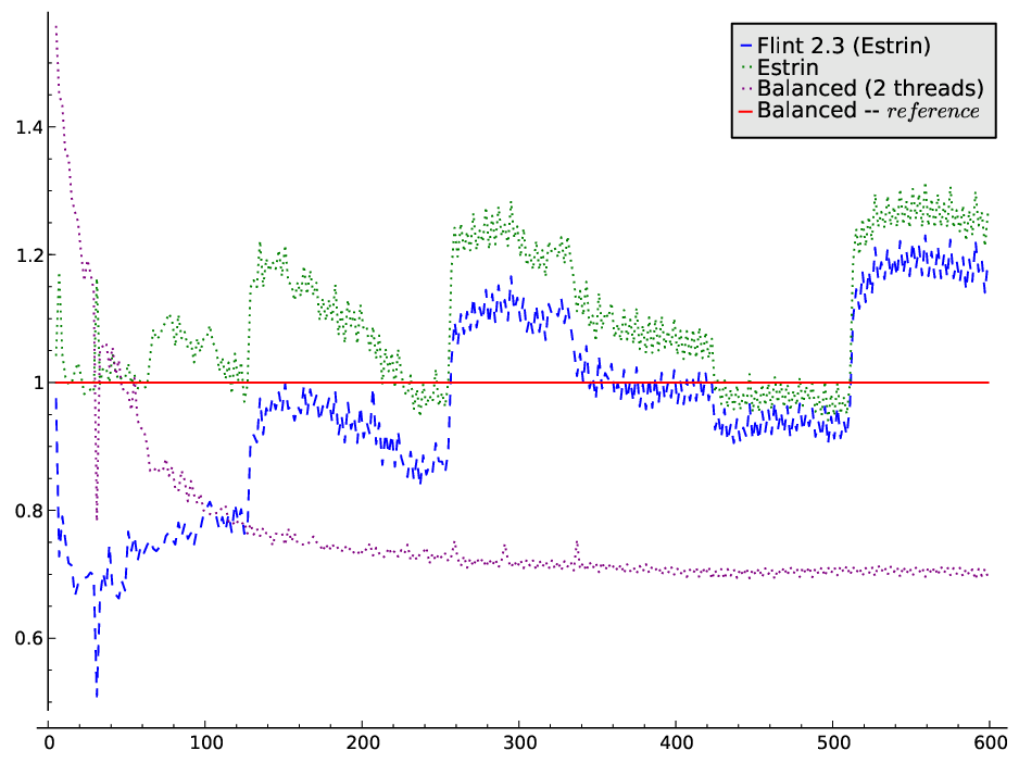
The Estrin scheme is a divide and conquer algorithm well suited to evaluate polynomials on elements whose size increases linearly with each multiplications ([BK75, BZ11]). These elements include multiple precision integers or univariate polynomials. However, the computation time of evaluating $\mathcal{T}_{p}^{E}$ reaches thresholds when the number of terms of $p$ is a pure power of $2$ (see Figure 1 in Section 3).

We introduce in this library a new evaluation scheme that avoids the time penalty of the classical divide and conquer. It is defined by the balanced function scheme.

\text{Balanced: }B(k)=\lfloor\frac{k}{2}\rfloor

Example 1.6.

[continued] The balanced divide and conquer evaluation trees contains lower partial degrees in this example.

1.3 Lazy height

We associate to each node of the tree a lazy height, that will determine the number of temporary variables required during the evaluation. In particular, the lazy height must be kept as low as possible. Classically, the height of a node is always greater then the height of its children. In our case, the lazy height of a node is greater than the lazy height of its children only if it has two or more children. In particular, this ensures us that for any tree, the maximal lazy height is at most logarithmic in the number of nodes.

Definition 1.7.

Let $N$ be a tree node. The lazy height of $N$ , denoted $lh(N)$ , is defined recursively. Let $C_{1},...,C_{k}$ be the child nodes of $N$ such that $c_{1}>_{t}\cdots>_{t}c_{k}$ .

lh(n)=\left\{\begin{array}[]{cl}0&\text{ if $N$ has $0$ or $1$ child.}\\ \displaystyle\max_{2\leq i\leq k}(lh(C_{i}))+1&\text{ otherwise.}\end{array}\right.

Example 1.8.

Consider again the polynomial $p=3x^{8}-x^{7}+2x^{6}+x^{5}-4x^{4}+9x^{3}-3x^{2}-2x+1$ . In the case of Hörner scheme, the maximal lazy height of the associated evaluation tree is $0$ , whereas its classical height is $8$ . The lazy height associated to the Direct scheme is $1$ . And we can check that the Estrin scheme and the Balanced scheme have both maximal lazy heights $1$ .

2 Evaluation

2.1 Coefficients walk

Once the tree data structure has been computed, the evaluation can be done efficiently. If $p$ is a univariate polynomial of degree $n$ , we can use the following pseudo-code.

for i from 0 <= i < n:

N = nodes[i]

c, d, h = N.coefficient, N.partial_degree, N.lheight

p = (m[h] + c)*x^d

m[h] = 0

if i == n: return p

elif i < n: m[N.parent.lheight] += p

If the values $x^{d}$ have been precomputed (see next Section), each step costs one multiplication and one addition. The mutable variables are $p$ and $m[0],...,m[L]$ , where $L$ is the lazy height of the root node. Their number is at most $O(\log n)$ .

2.2 Powers computation

The powers $x^{d}$ appearing in the evaluation loop can be computed several times for the same $d$ . In order to optimize the evaluation, these powers can be precomputed using fast exponentiation methods.

Assume that $p$ is a dense univariate polynomial of degree $n$ . Table 2.2 shows that the balanced scheme, as well as the Estrin scheme, require at most a logarithmic number of different powers to compute.

References

- [BK75] Richard P Brent and HT Kung. 0 ((n log n) 3/2) algorithms for composition and reversion of power series. Analytic computational complexity, pages 217–225, 1975.
- [BZ11] Marco Bodrato and Alberto Zanoni. Long integers and polynomial evaluation with estrin’s scheme. In Symbolic and Numeric Algorithms for Scientific Computing (SYNASC), 2011 13th International Symposium on, pages 39–46, 2011.
- [Est60] Gerald Estrin. Organization of computer systems: the fixed plus variable structure computer. In Papers presented at the May 3-5, 1960, western joint IRE-AIEE-ACM computer conference, pages 33–40. ACM, 1960.
- [Mul06] Jean-Michel Muller. Elementary functions. Computer Science. Birkhäuser Boston, 2006.