Linear-Time Recognition of Probe Interval Graphs
Abstract
The interval graph for a set of intervals on a line consists of one vertex for each interval, and an edge for each intersecting pair of intervals. A probe interval graph is a variant that is motivated by an application to genomics, where the intervals are partitioned into two sets: probes and non-probes. The graph has an edge between two vertices if they intersect and at least one of them is a probe. We give a linear-time algorithm for determining whether a given graph and partition of vertices into probes and non-probes is a probe interval graph. If it is, we give a layout of intervals that proves this. We can also determine whether the layout of the intervals is uniquely constrained within the same time bound. As part of the algorithm, we solve the consecutive-ones probe matrix problem in linear time, develop algorithms for operating on PQ trees, and give results that relate PQ trees for different submatrices of a consecutive-ones matrix.
1 Introduction
The intersection graph for a collection of sets has one vertex for each of the sets and an edge between two vertices if the corresponding sets intersect. An interval graph is the intersection graph of a set of intervals on a line. The set of intervals constitutes an interval model of the graph. Figure 1 gives an example. Interval graphs play an important role in many problems, see [7, 10, 12].

The problem of recognizing whether a graph is an interval graph played a key role in the 1950’s in establishing the linear topology the fine-scale organization of genetic information in DNA [2]. The linear topology of a DNA molecule had been known since 1953, when it was described by Watson and Crick. In addition, it was known that the collection of genes had a linear arrangement along the chromosome, since this arrangement could be inferred from recombination frequencies of alleles.
This was not enough to establish what we now know, which is that the genetic information in a chromosome is written in its entirety onto a single DNA molecule (actually, two identical DNA molecules called sister chromatids). What was known at that time did not exclude the possibility that the fine structure of the chromosome was organized around multiple independent DNA molecules or one with small branches, giving it a tree-like topology that only appeared to be linear on a large scale.
To test the hypothesis that the fine structure was linear, Seymour Benzer isolated 145 mutant strains of a bacteria-infecting virus, T4 [2]. He further hypothesized that each mutation occupied a contiguous region of the genome, which would be an interval of the genome if the topology was indeed linear. The test of these hypotheses consisted of finding a method for determining which pairs of mutations occupied intersecting regions of the genome, and then testing whether the derived intersection graph was an interval graph.
By themselves, the strains are not viable. When bacteria are infected with two of the strains, however, the viruses can recombine their genomes to assemble the original viral genome, giving rise to viable viruses, provided that the regions occupied by their two mutations do not intersect. By infecting bacteria with a pair of strains and determining whether viable viruses arose, he was able to deduce the presence or absence of an edge in the intersection graph with high accuracy. He found an interval graph on 144 of the 145 strains that was consistent with thousands of tests. The anomalous strain had to be excluded when it was found to have two mutations that were not contiguous.
The fraction of all graphs that are interval graphs on 144 vertices is minuscule, so this was a strong test of the hypothesis. The interval model he found for the graph gave one possible linear arrangement of the intervals occupied by the mutations, but this was not uniquely constrained by the graph, hence by the data.
His paper gives the first characterization of interval graphs, based on combinatorial properties of their adjacency matrices, together with a heuristic for recognizing whether a graph is an interval graph. According to an acknowledgment at the end of the the paper, the characterization of interval graphs and the heuristic he used for recognizing them was due to the prominent biochemist Leslie Orgel of Cambridge, who suggested it to him in a personal communication. As far as we know, the original characterization has not previously been attributed to Orgel in the graph theory literature.
This ignited considerable interest in the combinatorial study of interval graphs. Lekkerkerker and Boland gave a characterization in terms of forbidden induced subgraphs in 1962 [14]. It also sparked a search for efficient algorithms for determining whether a graph is an interval graph [9] and producing an interval model if it is. Booth and Lueker gave the first linear-time algorithm for the problem in the 1970’s [4]. Their algorithm determines whether the graph uniquely constrains the linear arrangement of the intervals.
A (partitioned) probe interval graph [20] (also called interval probe graph) is a graph in which the vertex set is partitioned into probes and non-probes. It is a generalization of intersection graph of an interval model, such that the graph has an edge between two vertices if their intervals intersect and at least one of them is a probe. Information about intersections of non-probe intervals is missing. Such a model is a probe interval model of the graph.
There has been quite a bit of work on topological and combinatorial properties of these graphs; see [12] for a survey. The motivation that initially gave rise to interest in the class was for physical mapping of genomes [29, 27, 28]. Rather than using mutations to deduce intersections, small fragments of single-stranded DNA from a region of a genome were cloned and embedded in a filter, and then tested against probes taken from the complementary strands to see which probes hybridized (bonded) with them. Hybridization indicates that the strands share a section that encodes for the same sequence of base pairs. If this sequence is long enough, it occurs on a unique interval of the genome, and therefore indicates that the strands come from intersecting intervals. Only a subset of the fragments were used as probes. The intersections inferred by the procedure were represented by a probe interval graph, since no direct information about hybridization between non-probes was available in the experimental data. The possibility of deducing a probe interval model from the graph, especially if it was uniquely constrained, provided a possible way to infer the linear arrangement of the fragments.
At the time, no efficient algorithm for deducing a probe interval model was known. The possibility that one might not exist was recognized as an obstacle to the approach [20]. In [28], a heuristic based on breadth-first search was instead applied to the probe interval graph in the hopes of finding a chordless path in the probe interval graph that consisted of intervals that spanned the region of interest. An efficient algorithm for constructing probe interval models, had it been available, could have solved this problem reliably.
A polynomial algorithm for the recognition and construction of probe interval models was first given by Johnson and Spinrad [13], who gave an bound. Using a different approach, McConnell and Spinrad gave an algorithm [18]. Uehara claimed an algorithm [26] that checks whether the model is unique, though some of the details have not been fully described.
In this paper, we give the first linear-time algorithm for the problem. That is, the input is a graph , where the is a partition of the vertices into probes and non-probes. The algorithm determines whether there exists a probe interval model of consistent with this partition of the vertices into probes and non-probes. If there is, the algorithm returns such a model. The algorithm also determines whether the layout of the model is unique, according to a slight generalization of a definition of uniqueness that is well-known in the case of interval graphs, and suitable for deducing the arrangement of intervals in a genome. This work appeared in preliminary form in [19].
All of the above algorithms take as input a graph whose vertex set is partitioned into probes and non-probes. Chang et al. [6] consider the problem of recognizing this graph class when this partition is not given.
The original motivating application to biology has been superseded by more reliable and economical techniques. However, hybridizing pairs continue to be of interest for inferring whether intervals occupied by DNA fragments intersect [8], giving rise to intersection graphs.
In some cases, the intersection graphs continue to be modeled by probe interval graphs, rather than full interval graphs. For example, in contig scaffolding, there are two kinds of segments of the genome, contigs and intervals with paired-end tags [24]. The sequence represented by a contig is known. Only small sequences at the extreme ends of a tagged intervals are known, however; these are the paired-end tags. The intersections of contigs with each other and with paired-end tag intervals can be deduced. The tags are small compared to the lengths of their intervals. Therefore, when two of these intervals intersect, their end tags are unlikely to intersect, and the intersection of their intervals cannot be inferred directly. The graph given by the hybridization data is therefore modeled by a probe interval graph, where the contigs are the probes and the paired-end tag intervals are the non-probes.
Our algorithm would probably have been more useful for Benzer than Booth and Lueker’s, had these algorithms been available at the time, because he did not have the resources to perform all experiments needed to construct the full interval graph on mutations.
An obstacle to the usefulness of efficient algorithms for construction of interval models from hybridization data is that, at the time of this writing, hybridization data are prone to many false positives and false negatives. This corrupts the experimentally derived graph by adding or removing edges in the true intersection graph, and with high probability, this will give rise to a graph that is no longer an interval graph or probe interval graph. This is one reason that the proposed method of [27, 29] never become competitive with alternative sequencing techniques. Advances in in the accuracy of detecting intersections, either by hybridization or by some unforeseen method, before our algorithm for constructing probe interval models, or Booth and Lueker’s algorithm for constructing interval models, are very useful in physical mapping or sequencing. Benzer’s methods, however, illustrate that it may be difficult to foresee clever future laboratory methods that could give rise to highly accurate intersection data in the future.
Despite impracticality of applying it to noisy biological data, the algorithm of Booth and Lueker continues to be studied by people working with hybridization data, because of the structural insights it gives about the graph class. The concepts it uses, such as the consecutive-ones property and PQ trees (discussed below) have given rise to methods that are more tolerant of errors in the data [22]. One contribution of our paper is to give analogous structural insights into the class of probe interval graphs.
A circular-arc graph is the intersection graph of arcs on a circle. Circular-arc graphs are a generalization of interval graphs; interval graphs are those circular-arc graphs that have a model where the arcs do not cover the entire circle. This generalization, which reflects constraints in cyclic scheduling problems, for example, is much less structured than interval graphs. For example, in interval graphs, the number of maximal cliques is bounded by the number of vertices, while in circular-arc graphs, it can be exponential in the size of the graph [25]. Interval graphs are a subclass of the class of perfect graphs, while circular-arc graphs are not. When Booth and Lueker developed their linear-time algorithm for recognizing interval graphs and producing interval models, Booth conjectured that the corresponding problems for circular-arc graphs would turn out to be NP-complete [3]. The conjecture was later disproved [25], and the first linear-time algorithm was given in [17].
The ability to find a probe interval model for a probe interval graph was an essential step in the result of [17]. The class of probe interval graphs was described independently in an early draft of that paper, before it was pointed out that it had previously been described in connection with a biological application. The paper used an algorithm for recognizing probe interval graphs and finding a probe interval models that is described in [18]. Even though the algorithm of [18] is not linear, it does not violate the linear time bound for the circular-arc graph recognition algorithm, since it operates on a graph whose size is sublinear in the size of .
One interpretation of a probe interval graph is that it is an interval graph where reports of adjacencies by non-probe vertices are missing or distrusted. Adjacencies between the trusted and the untrusted vertices can be obtained from the trusted vertices; only adjacencies between pairs of untrusted vertices are unknown. This interpretation is driven by applications that have been identified so far.
Another interpretation is that interval graphs are used to represent conflicts and compatibilities in scheduling problems. Their membership in the class of perfect graphs (see [10]) gives rise to efficient algorithms for finding maximum independent sets, maximum cliques, and minimum colorings [7], which correspond to sets of interest for finding efficient schedules. Probe interval graphs, which are also perfect graphs (see [20]), introduce a third possibility, which is that a subset of the jobs do not have a conflict even if their intervals intersect. For example, if some of the jobs require a dedicated resource for technical or security reasons, while others can share the resource, then the conflicts are modeled with a probe interval graph, where the jobs that require exclusive access are the probes and those that do not are the non-probes. A linear-time algorithm for finding a maximum clique and minimum coloring, given a probe interval model, is given in [12]. A consequence of our result is therefore a linear-time algorithm for minimum coloring and maximum clique, given the partitioned probe interval graph. An open problem is whether a maximum independent set and minimum clique cover can be found in linear time from the probe interval model.
A consecutive-ones ordered matrix is a 0-1 matrix in which 1’s in each row are consecutive. A consecutive-ones ordering of a 0-1 matrix is permutation of its columns that gives a consecutive-ones ordered matrix. A 0-1 matrix has the consecutive-ones property if there exists a consecutive-ones ordering of it. A family of subsets of a set has the consecutive-ones property if there exists an ordering of elements of such that each member of is consecutive. The two concepts are equivalent, since can be represented using one row for each , one column for each element of , and a 1 in row , column if set contains element of , and the resulting matrix has the consecutive-ones property if and only if the set family does. A consecutive-ones matrix is one that has the consecutive-ones property; it is not necessarily consecutive-ones ordered.
As part of their algorithm to recognize interval graphs, Booth and Lueker developed an algorithm to determine whether a matrix is a consecutive-ones matrix, and, if so, to produce a consecutive-ones ordering of it, in time proportional to the number of rows, columns, and 1’s in the matrix, given a sparse representation. We use this result extensively in this paper.
The consecutive-ones sandwich problem is an extension of the consecutive-ones problem, where each entry is 0, 1 or . An is a “don’t care”; it can stand for either a 0 or a 1. The problem is to find an assignment of 0’s and 1’s to the ’s such that the resulting matrix has the consecutive-ones property. Deciding whether this is possible is NP-Complete [11]. This fact was recognized as a possible obstacle to efficient construction of probe interval models in [20]. The consecutive-ones probe matrix problem is the special case where we require that the ’s form a submatrix (see also [5]). This is also a generalization of the consecutive-ones problem. We give an algorithm that takes time that is linear in the number of rows, columns, and 1’s in to find a solution or determine that none exists. This requires an efficient representation of that does not represent the ’s explicitly, and our solution gives an implicit assignment of 0’s and 1’s to ’s. The ’s can be assigned values explicitly, but the number of them might not be linear in the size of the input. In this paper, we develop methods for reducing the problem of constructing probe interval models to that of solving the consecutive-ones probe matrix problem.
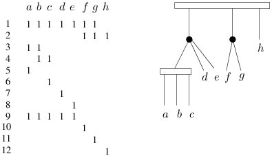
When Booth and Lueker’s algorithm determines that a matrix has the consecutive-ones property, it gives an implicit representation of all consecutive-ones orderings of a matrix, called a PQ tree. (See Figure 2.)
The leaves of the PQ tree are the one-element subsets of the set of columns of the matrix. The PQ tree gives all consecutive-ones orderings by constraining the orderings of children of internal nodes, as follows. Some of the internal nodes are labeled P nodes. For such a node every ordering of its children is permitted. Others are labeled Q nodes. For such a node, an ordering of its children is given; the only permissible orderings of its children are the given ordering and its reverse. For a PQ tree , let denote the set of all possible orderings of its leaves, given these constraints. uniquely determines . We consider different orderings of the PQ tree that are consistent with the constraints to be the same PQ tree. The algorithm of Booth and Lueker [4] either finds the unique PQ tree such that is equal to the consecutive-ones orderings of columns of a matrix , or determines that the matrix is not a consecutive-ones matrix. It is also easy to see that uniquely determines for any PQ tree. One way to see this is an algorithm we give below that, given , constructs a matrix whose consecutive-ones orderings are , which then has a unique PQ tree by Booth and Lueker’s result.
A significant part of our paper is devoted to developing general results about PQ trees and consecutive-ones ordered matrices that then allow us to derive our algorithm for probe interval graphs. We develop proof techniques and useful results about the relationships between the PQ trees of a matrix and those of its submatrices. See, for example, Section 4.3, and, for examples of applications, Sections 5.3.1 and 6). We give examples of how Booth and Lueker’s algorithm can be exploited as a black box for answering constraint satisfaction questions that do not correspond to ones that it had been originally designed for. See, for example, Sections 5.2.1 and 5.2.2.
Uehara claims a data structure for implicitly representing all possible probe interval models, though some details required to verify it are missing [26]. The time bound he gives for constructing it is . We develop a structure based on a pair of PQ trees that has this capability (Figure 11), and we construct it in time that is linear in the size of the graph.
2 Preliminaries
2.1 Notation
Except for some additional definitions, we use standard terminology and conventions from [7]. For example, that text states that the space requirement of the adjacency-list representation of a graph is , since it requires that many integers and pointers (words of memory in the RAM model), even though the number of bits required is . We use the RAM model in this paper for measuring space requirements, not just time requirements.
Given a graph, we let denote the number of vertices and the number of edges. We will assume the standard adjacency-list representation of a graph. Let denote the open neighborhood of , that is, the set of neighbors of in , and let denote its closed neighborhood, that is, .
By , we denote a probe interval graph with probes and non-probes . Let denote the vertex set. If is a nonempty subset of , let denote the subgraph of induced by , together with the classification of members of as probes or non-probes.
If is a set, let denote . If is a collection of sets, let denote . If is a graph and is a vertex, let denote . More generally, if , let denote .
If is a 0-1 matrix, let and denote its rows and columns, respectively. If is a subset of its rows, and is a subset of its columns, denotes the submatrix given by rows of and columns of . When we wish to restrict only the row set, we denote this ; it is implied that columns are . When we wish to restrict only the column set, we denote this ; it is implied that the row set is the . If is a column of , then we let denote .
We will often treat the columns of a 0-1 matrix as sets, where each column is the set of rows in which the column has a 1. A shortcoming of this convention is that, unlike a dynamic list, a set has no identity independent of its contents. We want a column to retain its identity when we add or remove a row from the matrix, even though the set it represents may change. Also, if two columns represent the same set, we want them to have separate identities, which they retain even when we permute the column order.
We therefore assume that each column has an identity separate from its current contents, much like a dynamic list. Taking a submatrix of can be seen as an operation on column lists. This allows us to say that and have different sets of rows but have the same column set. If is a column of , we let denote the set of rows where the column has 1’s. Note that . If is understood, we let denote . Rows are handled in a symmetric way; if is a row, denotes the set of columns of where the row has a 1, and if is a set of columns of , . Though this notation is convenient in mathematical expressions, we will sometimes ignore the distinction between a column and the set it represents in English sentences when the meaning is clear. For example, we can say that column is a subset of another column instead of the more formal for some such that .
A sparse representation of a binary matrix can be obtained by giving to each 1 a pointer to the next and preceding 1 in its row and the next and preceding 1 in its column. The size of the representation, as measured on the RAM model, is proportional to the number of rows, columns and 1’s and we consider an algorithm to run in linear time if it runs in time proportional to this size. Using elementary methods, such a representation can be obtained in linear time from a list of the positions of nonzero elements in each row or in each column. The order of rows and columns can also be permuted arbitrarily in linear time. A submatrix can be represented with ordered lists of pointers to a subset of rows and columns.
2.2 Classes of graphs and matrices
We define the cliques of a graph to be its maximal complete subgraphs. We assume that the vertices of a graph are numbered from 1 through . A clique matrix of a graph is a 0-1 matrix with one row for each vertex, one column for each clique, and a 1 in row , column if vertex is a member of clique . In this paper, we consider two clique matrices to be equal if and only if they are equal in the standard sense of matrix equality in linear algebra. This differs from some papers that refer to the clique matrix, reflecting the view that the purpose of the matrix is to represent the family of cliques, and the order of columns is unimportant. By our convention, an interval graph with cliques has clique matrices, all of which have the consecutive-ones property but not all of which are consecutive-ones ordered.
A vertex is simplicial if is a complete subgraph; in this case, must be a clique.
A chordal graph is a graph with no induced cycle of size greater than three. A chordal graph has cliques, and the sum of their cardinalities is , so a sparse representation of a clique matrix takes space. It takes time to find a sparse representation of a clique matrix of a chordal graph by the algorithm of Rose, Tarjan and Lueker [23].
Booth and Lueker’s algorithm [4] for recognizing interval graphs uses the algorithm of Rose, Tarjan and Lueker either to determine that the graph is not chordal, in which case it is not an interval graph, or else to produce a sparse representation of a clique matrix.
It then uses the fact that a graph is an interval graph if and only if its cliques have the consecutive-ones property. The central element of their recognition algorithm is an algorithm for either finding a consecutive-ones ordering of a 0-1 matrix, or else determining that none exists. They apply this to a clique matrix of the chordal graph to determine whether it is an interval graph. Figure 3 gives an example.
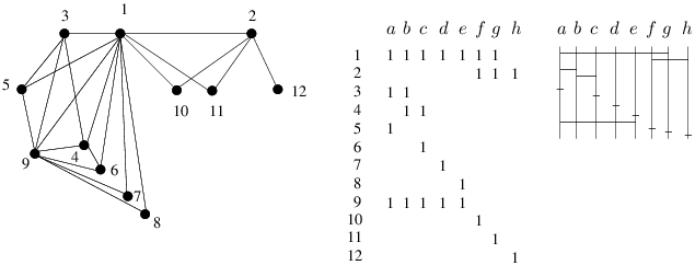
To see why a graph is an interval graph if its clique matrices are consecutive-ones matrices, note that the consecutive-ones ordering of a clique matrix defines an interval model: the interval for each vertex extends from the first to the last column of the block of consecutive ones in its row. Two vertices of a graph are adjacent if and only if they are members of a common clique, so two of these intervals intersect if and only if their vertices are adjacent. Thus Booth and Lueker’s algorithm produces an interval model whenever the input graph is an interval graph.
To see why the clique matrices of every interval graph have the consecutive-ones property, let be an interval graph. There exists a set of intervals on the line, one for each vertex, whose intersections give the edges of . For each clique of , the intervals corresponding to are pairwise intersecting. Any set of pairwise intersecting intervals must have an intersection point in common; this is known as the Helly property. Associating one such point on the line for each clique gives a left-to-right ordering of the cliques. For each vertex, the cliques that contain it are those whose associated points lie in the vertex’s interval. These cliques are consecutive in the left-to-right ordering, so this ordering of the cliques is a consecutive-ones ordering. For example, in Figure 1, the cliques from left-to-right are , and for each vertex, the cliques that contain the vertex are consecutive in this ordering.
An important fact for our purposes is that Booth and Lueker’s algorithm for finding a consecutive-ones ordering can operate on an arbitrary 0-1 matrix, not just a clique matrix of a chordal graph. Its input is a sparse representation of the matrix, and it takes time proportional to the number of rows, columns, and 1’s in the matrix. If a 0-1 matrix is consecutive-ones ordered, let the left endpoint of a row be the column of its first 1, the right endpoint be the column of its last 1, and the row’s interval the block of columns where it has 1’s.
For the consecutive-ones probe matrix problem, we seek to represent the inputs in space proportional to the number of rows, columns, and ’s in the probe matrix. In other words, we do not have to represent the ’s explicitly. Let be the submatrix of the probe matrix whose rows are the rows that do not have ’s, and whose columns are all columns of . Let be the submatrix of whose columns are the columns that do not have ’s, and whose rows are all rows of . The columns of are a subset of the columns of , and the rows of are a subset of the rows of . We represent the input to the problem using sparse representations of and , neither of which contain ’s.
A solution is any a consecutive-ones ordering of columns of , hence of the columns of , such that the subsequence given by columns in is also a consecutive-ones ordering of . This assigns a position to each column of among columns of . An is implicitly a 1 if it occurs between two 1’s from columns of in the ordering of columns of . Since is consecutive-ones ordered, this gives a consecutive-ones ordered matrix. We solve the problem in time linear in the number of rows, columns, and 1’s in and . This time bound does not allow us to explicitly assign 1’s to the ’s; they are implied by the column order. This nevertheless allows linear-time construction of a simple data structure that allows lookup of the value in any row and column of , by storing the column number of the first and the last 1 of every row.
3 Overview
At various points, our algorithm may find that a required property is not met, when it must hold if is a probe interval graph. In this case, we may reject . For instance, if is a probe interval graph, then the subgraph induced by the probes is an interval graph, so a clique matrix of this subgraph must have the consecutive-ones property. An initial step is to find a consecutive-ones ordering of this matrix, which is required in order to carry out the next steps of the algorithm. If does not have one, then we can reject and halt. We therefore assume that is a probe interval graph and use this to prove properties that are required at each step. If we cannot perform the operations as described at the step because the properties do not hold, we reject and halt. The algorithm also tests for required properties before a step if their absence could undermine the time bound before the problem is noticed. If it does not reject , the algorithm constructs a probe interval model of .
The notion of a model of an interval graph generalizes easily to probe interval graphs. Henceforth in this paper, we use the following convention:
Definition 3.1.
A probe interval model of a probe interval graph is a consecutive-ones-ordered matrix that has one row for each vertex, such that two vertices are neighbors in if and only if their rows intersect and at least one of the vertices is a probe. An interval model of an interval graph is a probe interval model that has no non-probes.
The consecutive-ones ordered clique matrices of an interval graph are not the only models of an interval graph that satisfy Definition 3.1. Between any two consecutive cliques and , it is easy to see that a column can be added such that is a subset of or of and supersets of without affecting the represented graph.
Notice that the probes in each column induce a complete subgraph in , but the vertices in a column do not induce a complete subgraph if the column contains more than one non-probe, since non-probes are nonadjacent. The Helly property requires that a each clique of be a subset of some column in every probe interval model.
Booth and Lueker treat consecutive-ones ordered clique matrices as the “canonical” or “normal” representation of an interval model. Let us call this an interval model in normal form. Restricting the focus to this normal form has distinct advantages. This representation distills down the information that the graph gives about possible structures of models, without representing arbitrary details that cannot be deduced from . Every one of these models is a consecutive-ones ordering of a single model, allowing the PQ tree to give a representation of all of them. They gives a precise definition to what it means for the model to be uniquely constrained: the model is unique, up to reversal of columns. Also, the number of 1’s in the clique matrix is , and this is not true for arbitrary models. Models that are not clique matrices are implicitly represented by those that are.
We therefore also seek a generalization of this standard form to probe interval models. If is a probe interval model, let the probe set in a column denote the probes that are members of the column. A contraction of a row in a probe interval model is the operation of changing its first or last 1 to a 0, resulting in a shorter interval for the row’s vertex. A row is taut if contracting it changes the represented neighborhood of the row’s vertex. A probe interval model is taut if every row is taut. Two consecutive columns in a model can be merged if they can be replaced with their union without changing the represented probe interval graph. A model is minimal if no two consecutive columns can be merged. Two such columns can be merged if one is a subset of the other, or if they have the same probe set, since making non-probes subsets of a common column does not represent them as adjacent.
Definition 3.2.
A probe interval model is a normal probe interval model if it is taut and minimal.
It is easy to see that in the special case of an interval model, where there are only probes, a model is a normal model if and only if it is a consecutive-ones ordered clique matrix. Therefore, a normal probe interval model is a generalization of the an interval model in normal form. We show below that, just as in the case of interval graphs, every probe interval graph has a normal model. As in the case of clique matrices, a normal model has 1’s. This is important for the time bound. Note that is an interval graph. Each clique of is a subset of exactly one column of every normal model of (4.4), just as in the special case of normal interval models. If a probe interval graph has no simplicial non-probes, the normal models are the consecutive-ones ordering of a single normal model (4.13), and the PQ tree of this model therefore gives a representation of all normal models, just as in the case of normal interval models.
Unfortunately, this is not true of probe interval graphs that have simplicial non-probes. The difficulties posed by simplicial non-probes were previously identified by Uehara [26]. That a PQ tree does not suffice to represent all probe interval models of a partitioned graph is illustrated by Figure 4.

We give an algorithm for finding whether a probe interval graph has a unique normal model, up to reversal of column order.
Every column of a normal model contains an endpoint of a row. Let the clique columns be those that contain a clique of . We show that a column is a clique column if and only if it contains both left and right endpoints of members of . Let be the simplicial non-probes. Let the simplicial columns be those that are not clique columns and that only contain endpoints of members of . The remaining columns, the semi-clique columns, contain right endpoints from and left endpoints from from , or vice versa. The non-simplicial columns are the clique and semi-clique columns.
At the highest level, the strategy is to build up increasingly larger matrices that are submatrices of normal models of increasingly larger subgraphs of . At each step, we permute the columns from the matrix produced by the previous step so that it is a submatrix of a normal model of the next larger subgraph, then add rows and columns to obtain a normal model of the larger subgraph. We halt when we either discover along the way that is not a probe interval graph, or else when we return a normal model of .
The reader may find it helpful to refer to the following sequence of matrices when reading the paper. The sequence is an outline of the steps of the algorithm.
- •
: This is a consecutive-ones ordered clique matrix of , which is an interval graph; we get this using the interval-graph recognition algorithm of [4]. If is a normal model of , some consecutive-ones ordering of is a submatrix of . In general, however, not every consecutive-ones ordering of is a submatrix of a normal model of .
- •
: The columns of are the clique columns of every normal model of , which is the same set of columns as that of . We obtain by adding one row for each member of to , filling in the remainders of the columns in the new rows, and finding a consecutive-ones ordering of the resulting matrix. Not all consecutive-ones orderings of are submatrices of normal models of , however.
- •
and : is obtained by adding constraint rows to . These correspond to columns that must be consecutive in any ordering of columns of that gives a submatrix of a normal model of . is a submatrix of a normal model of . The matrices and differ only in the order of their columns. We let denote their column set.
- •
: This is a normal model of obtained by adding semi-clique columns to . This is possible to do because is a submatrix of a normal model of . We show that, ignoring members of , this gives the clique and semi-clique columns in every normal model of . Not all consecutive-ones orderings of columns of are submatrices of normal models of , however.
- •
: For some normal model of , some ordering of columns of is equal to the entire set of columns of . There is one column containing the probe set of each clique column and each semi-clique column. In addition, there is one column for each neighborhood of a simplicial non-probe that is not the probe set of a clique column or a semi-clique column. The latter set corresponds to the simplicial columns of a normal model of . Thus, for each , there is a column of equal to . The set of rows of corresponds to the set of probes .
- •
and : Let denote the clique and semi-clique columns in a normal model of . is a consecutive-ones ordering of the columns of . The set columns of is the same set of columns as of , and the set of rows of is the same set of rows as of . Note that the rows of are a subset of the rows of and the columns of are a subset of the columns of . We can find for some model of by solving the consecutive-ones probe matrix problem using in the role of and in the role of , where and are the matrices from the definition of the consecutive-ones probe matrix problem (Section 2.2). Since we need an time bound, and not a time bound proportional to the number of 1’s in and , we can explicitly fill in the ’s that are 1’s, giving a sparse representation of . This is because is a submatrix of a normal model of , so it has 1’s.
The probe set in each simplicial column is a subset of a clique of . It follows that is a model of . It is not a normal model of . However, for each , it now has a column equal to , so can be placed in this column and its neighborhood is correctly represented. Doing this for all yields a normal model of .
Let us assume that the members of occupy the top rows of a model, followed by members of , followed by the members of . This is accomplished with a suitable numbering of the vertices, which fixes the row order in all models.
For each probe , let denote the set of cliques of that are subsets of . These are the set of cliques that contain as a member. Generalizing this, for each non-probe , we let denote the set of cliques of that are subsets of . Since the sets represented by columns of are the cliques of , we may represent and with the corresponding sets and of columns of . The set is given for each probe , and using the fact that is consecutive-ones ordered, we can efficiently find for each non-probe , as described in Section 4.4.
We partition the set of non-probes into three sets: for a non-probe , if , if it is non-simplicial and , and if it is simplicial. Note that if , it is not simplicial, so is a partition of .
To find , we add one row to for each , equal to . That this completes the clique columns of every normal model of follows from the Helly property and the appearance of each clique of in a unique column. For each vertex of , the row is empty. is any consecutive-ones ordering of the resulting matrix.
For each , probes in columns in are neighbors of , since they belong to cliques that are subsets of ’s neighborhood. , when interpreted as a probe interval model, represents these adjacencies. is not a complete model of ; for a neighbor of , it can be that only occurs in columns that also have non-neighbors of . Therefore, and do not intersect in , and fails to represent their adjacency. Let us call these unfulfilled adjacencies in .
These are the reason semi-clique columns also occur in normal models of . Such an unfulfilled adjacency must be resolved by inserting a semi-clique column where and can meet. This requirement places additional constraints on the ordering of columns of . It must be such that no columns intrudes between the intervals for and . This would block them from meeting each other in a new column, since one of them would have to cross . Since is not a member of or of , it contains non-neighboring probes for both and , and having one of them cross would misrepresent the graph.
We can avoid this by adding a constraint row to , equal to for each such pair, and getting a consecutive-ones ordering of the resulting matrix. (See Figure 7). A variant of this trick is required when , since then is empty.
Doing this for all unfulfilled adjacencies would exceed the bound. Fortunately, many of the constraints are redundant. We add a constraint only for representative pairs of unfulfilled adjacencies, and the omitted constraints are redundant (Figure 8). This adds 1’s to the matrix, and a consecutive-ones ordering of it gives .
Now that they have helped order the columns of , we delete the constraint rows to obtain , which is a submatrix of a normal model of .
We can now extend to the model of by inserting the semi-clique columns between each pair of consecutive columns of (Figure 10).
A normal model can then be built for using a solution to the consecutive-ones probe matrix problem, as described in the last point above. A key tool in our solution of the consecutive-ones probe matrix is the idea of the restriction of the PQ tree of a matrix to the one-element subsets of a set of its columns. This is a type of homomorphism that preserves the constraints consecutive-ones orderings of impose on the relative orderings of columns in . (See Figure 6.) A special case of this operation has been described in [16] and in [15], but only for certain sets of columns such that is the PQ tree of . The general solution is trivial to compute (Algorithm 1). The concept shows promise as a tool for proofs. The strategy for applying it to the consecutive-ones probe matrix problem is outlined in the caption of Figure 11.
4 Initial steps and observations
We can run the recognition algorithm separately on each connected component of to produce disjoint probe interval models for the components. The collection of these is a probe interval model of . If any component fails to be a probe interval graph, then fails to be a probe interval graph. This reduces the problem to that of deciding whether a connected graph is a probe interval graph, and producing a model if it is. Henceforth, we will assume that is connected.
4.1 Variations on radix sorting
Given a collection of lists of integers from , whose sum of lengths is , we may sort each list by sorting all the elements of all the lists in a single radix sort using set number as primary sort key and element value as secondary sort key. This takes time. We can sort the adjacency lists of a graph in linear time, for example. Also, we can sort the collection of the lists lexicographically in time even though they have different lengths [1]. Thus, we can sort the rows or columns of a matrix lexicographically in linear time, given a sparse representation.
Variations of this that we will use are the following. Suppose we are given groups of lists of integers from 1 through , and the sum of lengths of the lists of integers is . We can sort each list of integers, all lists lexicographically, and then, using a stable sort, segregate this list back into the groups. This gives each of the groups, sorted lexicographically, in time. Since each list of integers is sorted, we may eliminate any duplicate lists in any of the groups, also in time. If, instead of sorting the lists lexicographically in this sequence of operations, we sort the lists by length, we get each of the groups sorted by length. We can then determine whether the elements of each of the groups induce a chain in the subset relation, in time.
4.2 Properties of normal models
Lemma 4.1.
For every probe interval graph , there exists a normal probe interval model of .
Proof.
Let be an arbitrary probe interval model of . If some row is not taut, we may change an endpoint of its interval from 1 to 0 without affecting the represented graph. If two consecutive columns can be merged without changing the represented graph, we merge them.
We iteratively perform one of these operations until none of them can be performed. Since each operation reduces the number of 1’s in the matrix, this process eventually results in a normal model, and since none of the operation changes the represented probe interval graph, it is a normal model of . ∎
Lemma 4.2.
In every normal model of a connected probe interval graph that has more than one vertex, every column has a nonempty set of probes.
Proof.
If is a column with an empty set of probes, cannot be the endpoint of any vertex, since it would either fail to be taut or be a simplicial non-probe with no neighbors, contradicting connectedness of the graph. ∎
Lemma 4.3.
In every normal model, each non-probe resides in a single column if and only if it is simplicial.
Proof.
If a non-probe occurs in only one column , its neighbors are , which form a complete subgraph due to their presence in a common column, and is simplicial. If a simplicial non-probe has a 1 in more than one column, the Helly property dictates that one of the columns has as its probe set, and ’s 1’s in the other columns can be deleted without affecting the represented graph, contradicting the tautness of the model. ∎
A probe may occur in only one column without being simplicial, since its non-probe neighbors are nonadjacent to each other.
Lemma 4.4.
In a normal model, each clique of is a subset of exactly one column.
Proof.
Each clique of must be a subset of at least one column by the Helly property of interval models. Suppose a clique is a subset of more than one column. By consecutiveness of 1’s in each row of , the intersection of these rows is consecutive. The columns in this intersection all have as their probe set. They can be merged, since the intervals that now meet and didn’t meet before are non-probes, contradicting the normality of the model. ∎
We can now fill out and justify the classification of columns as clique, semi-clique, and simplicial columns.
Definition 4.5.
A vertex that is a member of only one column in a model has degenerate endpoints; they are both . The endpoints of a vertex that is a member of more than one column are proper endpoints. A column of a model is a clique column if it contains a clique of . It is a left semi-clique column of if it has a proper right endpoint of a probe and a proper left endpoint of a non-probe, no left endpoint of a probe, and no right endpoint of a non-probe. A right semi-clique column is defined symmetrically. It is a simplicial column if it is not a clique column, contains a simplicial non-probe, and contains no endpoints of non-simplicial non-probes.
Lemma 4.6.
In a normal model, every column is a clique column, a semi-clique column, or a simplicial column.
Proof.
Let be a column and assume for contraction that it is not of one of these three types.
Suppose that is not the endpoint of any probe. If is a proper endpoint of some non probe then is not taut. If is a degenerate endpoint of a non-probe then it is a simplicial column. If is not an endpoint of any non-probe, then it can be merged with one of the adjacent columns without affecting the represented graph.
Suppose that is an endpoint of a probe . Without loss of generality, suppose it is a right endpoint. The column does not contains a left endpoint of a probe, since otherwise it would be a clique column. Since has no left endpoint of a probe, no member of can have its right endpoint in the column, as it would not be taut. If has no left endpoint at all in the column, then is not taut. Thus must have the left endpoint of a non-probe. If it contains the left endpoint of a member of , then it satisfies the definition of a left semi-clique. Otherwise, the left endpoints in the column belong to simplicial non-probes, and it is a simplicial column. In any of the cases we either get a contradiction to the normality of the model, or to the assumption that is not of one of the three types. Therefore, every column must be of one of the tree types. ∎
Though it would be convenient, we cannot require that every column have the endpoint of a probe. When a simplicial non-probe has as its neighbors the intersection of consecutive cliques of in the model, its column cannot contain the endpoint of a probe in the model.
Lemma 4.7.
In a normal model, no column is a subset of any other.
Proof.
Suppose a column is a subset of a column . Without loss of generality, suppose is to the left of . By consecutiveness of 1’s, if is the adjacent column to the left of . Thus, can be merged with without changing the represented graph. Since they are consecutive, this does not affect consecutiveness of 1’s in the model. ∎
We call a column that is not a clique column a non-clique column.
Lemma 4.8.
In a normal model , the probe set in every non-clique column is a proper subset of either the probe set of the next column to its left or of the probe set of the next column to its right.
Proof.
If and are consecutive columns with equal probe sets, they can be merged without affecting consecutiveness of 1’s or the represented graph. No consecutive columns have the same probe set.
Let be a non-clique column. A non-clique column cannot contain both left and right endpoints of probes. Without loss of generality, suppose that it does not contain the right endpoint of a probe. Then the set of probes in is a subset of the set of probes in the column to its left. Since consecutive columns cannot have equal probe sets, the probes in must be a proper subset of the probes in the column to its left. ∎
As we mentioned above, the matrix clique of an interval graph has columns and 1’s. It is not obvious that a model of a probe interval graph maintains this property, since there might be adjacencies among non-probes which are realized by the model but are not represented by edges in the graph. The next lemma shows however that for normal models this property holds.
Lemma 4.9.
If is a normal model of a probe interval graph , then has at most columns and 1’s.
Proof.
By Lemma 4.6, every column contains a left endpoint and a right endpoint. There are endpoints, so the number of columns is at most .
If a column has the endpoint of a probe , charge the 1’s in the column to . The number of 1’s in the column is bounded by the size of the closed neighborhood of . Over all columns, each probe is charged in at most two columns for the size of its closed neighborhood, so the number of 1’s in these columns is .
It remains to bound the number of 1’s in simplicial columns. Let be the simplicial columns. For each from 1 through , let be a probe with an endpoint in , or if it has no endpoint of a probe, let be a probe with an endpoint in a column next to . By Lemma 4.8, exists. Since contains no endpoint of a vertex in , by definition, every member of in is a neighbor of . The number of 1’s in is at most . Charge these 1’s to . Charge the 1’s in to an arbitrary probe in ; the rows where these 1’s occur are all neighbors of .
Each probe is charged times in the role of , for 1’s. A probe could be charged many times in the role of , but never twice for the same neighbor, since they are all simplicial and occur in only one column, by Lemma 4.3. The total number of these charges to is bounded by . Summing these charges over all probes gives the bound on the number of 1’s in columns . ∎
To derive more properties of normal models, we make use of the following insight, which is due to Zhang [27] (see also [20]). Let be the edges of . He defined the set and contains two nonadjacent vertices.. He then showed that an interval model of is a probe interval model of .
The strategy of a step of the probe interval graph recognition algorithm of Uehara [26] is to construct in order to find a model of . We cannot use that approach because does not have edges. A simple example of this is a graph with two nonadjacent vertices, and , and non-probes, each adjacent to and . The probe interval graph has edges, but in , the non-probes form a complete subgraph, so has edges.
However, we can derive structural properties of normal models from it by observing a normal model of is an interval model of a slight variation of . Therefore, even though this graph does not have edges, every clique matrix has 1’s.
Definition 4.10.
Let be the edges of . Let , and is either a clique of or contains two nonadjacent vertices. Let .
Lemma 4.11.
Every normal model of is a consecutive-ones ordered clique matrix of .
Proof.
Let be a normal model of . Let and be members of .
If is a clique of , their intervals must intersect at the only column that contains , by Lemma 4.4.
If contains two nonadjacent vertices, and , suppose without loss of generality that lies to the left of in . Let be the rightmost column of and be the leftmost column of . Since they are both adjacent to and , and must be contained in both and .
If is empty, then and contain no column in common, by Lemma 4.2.
Otherwise, is a complete subgraph that is not a clique of . Then is a proper subset of a clique . The intersection of and is a consecutive set of columns that do not contain . Suppose without loss of generality that the clique column containing lies to the left of , and that the right endpoint of is at the right endpoint of . By Lemma 4.3, is contained in more than one column of . The right endpoint of is not taut, contradicting the normality of the models, so this case cannot happen.
It follows that and are contained in a common column if and only if . For any pair where at least one of and is a probe, and are contained in a common column if and only if , by the definition of a probe interval model. is an interval model of , and so it is a consecutive-ones ordered clique matrix of as required. ∎
Lemma 4.12.
When interpreted as a probe interval model, every consecutive-ones ordered clique matrix of is a normal model of
Proof.
Let be a consecutive-ones ordering of a clique matrix of that is a normal model of . exists by Lemma 4.1 and Lemma 4.11. Let be a different consecutive-ones ordering of . Suppose that is not a normal model of . Then it can be turned into a normal model by a series of contractions of endpoints and merges of columns, as in the proof of Lemma 4.1. Each of these operations reduces the number of 1’s in the matrix. Therefore has fewer 1’s than , hence fewer 1’s than . Since is a normal model of , it is a consecutive-ones ordering of by Lemma 4.11, but and have different numbers of 1’s, a contradiction. ∎
Theorem 4.13.
The normal models of are the consecutive-ones orderings of a single matrix.
It follows that the set of all normal models of is given by the PQ tree of any one of these models.
According to the following theorem, ignoring members in , the collection of clique columns and the collection of semi-clique columns are each invariant over all normal models of , and no two clique or semi-clique columns are equal.
Theorem 4.14.
Let and be normal models of . No two clique or semi-clique columns of are equal. Let and be the collection of sets of vertices represented by clique and semi-clique columns of and , respectively. Then = .
Proof.
In a normal model of , let be the set of non-simplicial columns of . Let . Two probes that are contained in a simplicial column of are contained in a neighboring column , by Lemma 4.8. They remain adjacent when is deleted. Since a simplicial column contains no endpoints of non-probes of , non-probes that are contained in are contained in . They remain adjacent to the probes in when is deleted. Deleting a simplicial columns from does not change the graph represented by . Therefore, is a model of .
If is a clique column of , then it contains left and right endpoints of probes, and this remains true in . Every endpoint in the column is taut.
If is a semi-clique column, assume without loss of generality that it contains left proper endpoints of non-probes in . These non-probes are members of by Lemma 4.3, and contains left proper endpoints of non-probes in . It contains no right proper endpoints of non-probes in by the properties of semi-clique columns. Since no simplicial column contains a proper endpoint of a non-probe, contains no right endpoints of non-probes in . It contains right endpoints of probes in , and this remains true in . Every endpoint in is taut in .
Suppose two columns and of can be merged. Then they are consecutive and have the same probe set . Then since no clique column was deleted from to obtain , is the probe set in every column between and in , and all columns in this interval can be merged in , contradicting the normality of .
Unfortunately, it is not the case that every consecutive-ones ordering of a normal model of is a normal model if , due to the presence of simplicial non-probes. Figure 5 gives an example. There does not seem to be a single PQ tree for representing the possible models of a probe interval graph once simplicial non-probes are introduced.

4.3 PQ trees
We defined PQ-tree in Section 1. The classification of a node as a P node or a Q node is ambiguous if it has only two children. In this paper we adopt the convention of considering it to be both.
A PQ tree can be represented in space by letting each leaf carry a column identifier and each internal node carry a pointer to an ordered list of its children. Notationally, however, we denote each node in a PQ tree by a set, namely, the set of columns at leaf descendants. A leaf is a set whose only element is a column, and an internal node is the disjoint union of its children. The root is the set of all columns of the matrix. A consecutive set of columns in one consecutive-ones ordering must be consecutive in every consecutive-ones ordering if and only if is a P node or a union of consecutive children of a Q node.
Definition 4.15.
Let be a PQ tree and be a bijection from its leaves to , such that there is an allowed leaf order where each leaf is in position in the ordering. Then is a valid ordering for . Let the set of valid orderings for .
Definition 4.16.
If and are two PQ trees with the same leaf set, let denote that , denote that , and let denote that .
4.3.1 Restricting a PQ tree
Definition 4.17.
If is a bijection from a set to and is a nonempty subset of , then denotes the bijection from to such that for , if and only if . If is a set of permutations from to , then denotes .
Definition 4.18.
Let the restriction of a PQ tree to denote the PQ tree such that . If has leaf set , , and is a leaf, let denote .
That is well-defined can be seen from the following algorithm that computes it, in time linear in the number of nodes of . (See Figure 6.)
Algorithm 1.
Delete leaves that of are not in and each node that has no leaf descendants in . Then, for each node that has only one child , we can replace with in the ordered list of children at ’s parent, since imposes no constraints on the orderings of .

Lemma 4.19.
If is a consecutive-ones matrix and is a subset of its columns, then .
Proof.
Every submatrix of a consecutive-ones ordered matrix is consecutive-ones ordered, so for every , . ∎
4.3.2 A relationship between the PQ tree and the rows of the matrix
Let us say that two rows and properly overlap if , , or are all nonempty. The following is easily verified, and has appeared in [21], among other places:
Lemma 4.20.
If and are properly overlapping rows of a consecutive-ones matrix then , , and are consecutive in every consecutive-ones ordering of .
Definition 4.21.
[21] If is a consecutive-ones matrix on column set . Let denote and does not properly overlap any row of .
Lemma 4.22.
[21] If is a consecutive-ones matrix, is a node of or a nonempty union of children of a P node of .
Definition 4.23.
Suppose is consecutive-ones ordered. Let denote those members of that are consecutive in , that is, the nonempty consecutive sets of columns that do not properly overlap any row of .
Conceptually, the members of are those consecutive sets of columns whose order can be reversed to give a new consecutive-ones ordering of . This gives the following:
Lemma 4.24.
Let be a consecutive-ones ordering of a 0-1 matrix, and let be the corresponding ordering of its PQ tree. Then is a node of or a nonempty union of consecutive children of a Q node of .
and are equivalent representations of the constraints on the consecutive-ones orderings of columns of , but it is sometimes easier to prove properties of by expressing them in terms of .
4.3.3 Finding intersections of PQ trees
In [15], it is shown that if and are PQ trees with the same leaf set and is nonempty, then can also be represented with a PQ tree, denoted . This is easy to see: if is a matrix with as its PQ tree and is a matrix with as its PQ tree, then the matrix whose rows are the union of rows of and gives a matrix whose PQ tree is represents , unless this set is empty, which is the case if and only if does not have the consecutive-ones property.
Definition 4.25.
Let and be PQ trees with the same leaf sets. By , we denote the PQ tree such that , unless this set is empty, in which case we say the intersection of and is undefined.
Booth and Lueker showed that every consecutive-ones matrix has a PQ tree. We observe that the converse also applies, by the following construction, which, given a PQ tree , constructs a canonical matrix that has as its PQ tree.
- •
For each P node that is not the root, let be a row of ;
- •
For each Q node , let be the left-to-right order of the children. For every consecutive pair of children, let be a row of .
The correctness of this is immediate from Lemma 4.24.
Lemma 4.26.
If is the PQ tree of a matrix with columns and rows and 1’s, has 1’s and a sparse representation takes time to generate.
Proof.
Let be the PQ tree of a matrix with columns and rows and 1’s. In various sources, for example, in [21], it is shown that if is a Q node and and are consecutive children, then for some row of , is the least common ancestor of the members of , and . Since is a row of , we may charge the 1’s in this row to the 1’s in columns of in . The 1’s of in columns of are charged at most twice, at most once when appears in and at most once when appears in . Over all Q nodes, this charges each 1 in for at most two 1’s in .
It is also shown in [21] that if is a P node and not the root, then either there exists a row of such that , or there exists a row such that the least common ancestor of is a Q node parent , and . Charge the 1’s of the row corresponding to in to the 1’s in columns of in either or , whichever exists. Over all P nodes, this charges each 1 in for at most one 1 in . If the root is a P node, charge the 1’s in the corresponding row of to columns of the matrix. Thus, the number of 1’s in is at most the number of columns of the matrix plus three times the number of 1’s in , which is linear in the size of . ∎
An algorithm is given in [15] for finding this tree, but it uses sophisticated techniques and a roundabout set of reductions in order to get this time bound. Since we do not need this bound, we use the following straightforward method in time:
Algorithm 2.
Let be a matrix whose rows are the union of rows in and , and use Booth and Lueker’s algorithm to either generate the PQ tree of , which is , or determine that has no consecutive-ones ordering, in which case does not exist.
4.4 Finding , , and and for each
To partition into , , and , we begin by finding an arbitrary consecutive-ones ordered clique matrix of . That is, we find a normal model of . If none exists, we reject , since a requirement for to be a probe interval graph is for to be an interval graph.
We temporarily number the columns of from left to right. Let be a non-probe. We find for every the left endpoint and the right endpoint of . We keep the column numbers of these two endpoints, together with their side (left or right) in a list . We radix sort the concatenation of these lists with as the primary sort key, column number as the secondary sort key, and left versus right endpoint as the tertiary key. This gives each list in sorted order, with left endpoints in a column preceding right endpoints in the same column. The time required is proportional to the sum of cardinalities of these lists, .
We sweep through from left to right, keeping a running count of the number of neighbors of in the current column. Each time we encounter a left endpoint in we increment the counter, and each time we encounter a right endpoint we decrement it. Each time we encounter a right endpoint that follows a left endpoint, we compare the current value of the counter with the size of the clique represented by the column of , and include in if they are equal.
To find out whether is simplicial, we test whether the counter reached the size of at some point. If it passes this test, is a member of . If is empty but is not simplicial, it is a member of . Otherwise, it is a member of .
These procedures for take time proportional to for every non-probe . Summing over all , we have an bound for these operations. Summarizing, we get the following.
Lemma 4.27.
In linear time we can either split into and and find for every , or else determine that is not a probe interval graph.
5 Finding a normal model of
5.1 Finding
Recall that is the matrix with additional row for each non-simplicial non-probe.
Suppose . If clique of is a member of , then ’s row must have a 1 in column . This follows from the Helly property and the fact that there is only one column in a normal model that contains clique . If clique is not in , then ’s row cannot have a 1 in ’s column, since this would falsely represent as a neighbor of all members of clique . If is a probe interval graph, this matrix therefore gives us the clique columns of every normal model of . Note that the new rows for are empty sets; 1’s will be added to them later when new columns are added.
Let be the ordering of these columns in some normal model of . For each , must be consecutive in , since a submatrix of a consecutive-ones ordered matrix is consecutive-ones ordered. We find a consecutive-ones ordering of the columns, and if no such an ordering exists we reject .
For , let denote the probes whose rows in intersect ’s row. That is, is the neighbors of given by when it is interpreted as a probe interval model. There may be some vertices in . These are the unfulfilled adjacencies. They impose additional constraints on the consecutive-ones orders of , that allow semi-clique columns to be added to it to represent the unfulfilled adjacencies. From Theorem 4.14 it follows that every normal model of has some ordering of columns of as a submatrix.
5.2 Finding
Not every consecutive-ones ordering of is a submatrix of a normal model of . To find such an ordering, we add constraint rows to , and find a consecutive-ones ordering of the resulting matrix to reflect the constraints imposed by the constraint rows. This yields an ordering of that is a submatrix of a normal model of .
There are two types of constraints that must be reflected in , non-probe - probe binding constraints and probe - probe binding constraints.
5.2.1 Non-Probe - Probe Binding Constraints
Let and let . We know that , because . Since and are adjacent, we know that their intervals must intersect in any model of , and therefore must be consecutive in . Let us call this additional constraint a non-probe - probe binding constraint imposed by and . We can enforce this constraint by adding a new row equal to to . (See Figure 7.)

Adding such a constraint for every such and will make too large for our time bound. We show that a set of new rows with a linear number of 1’s is enough to enforce the non-probe - probe binding constraints.
Let be a non-probe of , and let be the leftmost column of and let be the rightmost in (the yet unknown matrix) . We can divide into the set of members that lie in columns to the left of and the set that lie in columns to the right of . For each , the rightmost column of is ; the only way for and to be adjacent is to meet at a semi-clique column between and in a normal model . Similarly, for each , the leftmost column of is . No element of is adjacent to any element of , and and each induce complete subgraphs, since they will contain a common endpoint of in . This implies that the same and arise for in every normal model of (up to interchange).
Recall that the vertices are numbered from 1 through . For two vertices and , let denote that either or that and has a smaller vertex number than does; the numbers serve as tie breakers. Let denote that or that .
Since the members of all end at the column to the left of ’s left endpoint and they all occupy consecutive cliques, it follows that for any , either or . induces a linear order in the relation. It has a unique a minimal member in this relation. For example, for in Figure 8, , , and is the unique minimal member of in the relation. Similarly, has a unique minimal member in the relation. Also, since and must lie on opposite sides of .
By similar reasoning, each for each probe , the relation on non-probes that is bound to has at most two nonadjacent minimal members and . Let us say that and are a representative bound pair if is a minimal bound neighbor of and is a minimal bound neighbor of in the relation. For example, in Figure 8, the two representative bound pairs are and .

We augment by adding a row for any representative pair that has ’s in the columns of . We show below that doing this for all representative pairs adds 1’s to the matrix, and enforces all non-probe - probe constraints, not just those for representative bound pairs.
Let us now consider how to find the representative pairs when we allow for the possibility that is not a probe interval graph. We have the endpoints of each vertex in . First, for each , we find its minimal bound neighbors in time proportional . We create a list of the unfulfilled neighbors of , and let be an arbitrary neighbor of in the list. For each unfulfilled neighbor in the list, we use the endpoints of the intervals corresponding to and to check whether is disjoint from , in which case it is not in , or contains , in which case it is in and we eliminate it from the list, or it is contained on , in which case is in , we eliminate it from the list, and let . This takes time per neighbor. If a fourth case occurs, we reject , since a necessary condition described above is not met. Otherwise, this gives us and the minimal neighbor in it for . If any unfulfilled neighbors remain, we find and the minimal member in it for in a similar way. If the list remains nonempty following this, then is not a probe interval graph. Summarizing:
Lemma 5.1.
In time, we can either reject , or find, for each , a partition of the unfulfilled neighbors of in into at most two sets, , , and label with , such that is the only minimal member of , is the only minimal member of , and .
If we do not reject , we have labeled each vertex with at most two minimal bound neighbors two minimal bound neighbors and . We identify as a representative pair if is also one of the minimal bound neighbors of . Similarly, we identify if as a representative bound pair of is also a minimal bound neighbor of . Since each vertex has at most two bound neighbors, there are pairs to perform this test on.
This gives the following:
Lemma 5.2.
In time, we can either reject , or find the representative pairs for the non-probe - probe binding constraints.
5.2.2 Probe - Probe Binding Constraints
Consider . In this case, hence . All neighbors of are unfulfilled. Then and its adjacencies must be represented exclusively by semi-clique columns.
Since , does not induce a complete subgraph in . Let and be two neighbors that are nonadjacent to each other. . Their intervals must intersect ’s in any model of . Therefore, must be consecutive in , so that semi-clique columns containing and , and and , can be placed in between and . This is a probe - probe binding constraint.
Again, however, doing this for all such pairs might add more than 1’s. It again suffices to add such rows for only a subset of such pairs .
In a model of , the 1’s in row therefore lie between two consecutive clique columns and . Suppose that lies to the left of . Let and let . The sets and satisfy , and . Also, since is not simplicial, neither nor is empty. Although we used a specific model to define and for , these sets are unique for every , up to interchange between the two.
As with the non-probe - probe binding constraints, for each non-probe , and are ordered by the relation. We find the minimal members and of and in the relation and make them bound partners.
For each probe, the bound partners can also be partitioned into at most two sets that are ordered by the relation, for the same reasons. A representative pair is two bound partners that are each minimal in the relation over bound partners of the other.
Let us now consider how to find the representative pairs when we allow for the possibility that is not a probe interval graph. We apply the algorithm from the end of the previous section to verify that for each , has at most two minimal bound neighbors in the relation. Similarly, for each probe , we verify that has at most two minimal bound partners in the relation. We reject if these conditions do not apply, as we have shown that they are necessary.
The number of bound partners of any probe is bounded by the number of neighbors in , so it is . This is over all probes. We assign at most two minimal bound partners and to each probe in time. For , we check whether is also one of its two minimal bound partners, and include as a representative pair if it is, and similarly for .
Proceeding as in the case of non-probe - probe constraints gives us analogues of Lemmas 5.1 and 5.2.
Lemma 5.3.
In time, we can either reject , or find, for each , a partition of the bound partners of into at most two sets, , , and label with , such that is the only minimal member of in the relation, is the only minimal member of in the relation, and .
A representative pair is two bound partners that are each a minimal bound partner of the other. Since each vertex has at most two bound partners, there are pairs to test for this condition.
Lemma 5.4.
In time, we can either reject , or find the representative pairs for the probe - probe binding constraints.
5.3 Finding
Let be a consecutive-ones ordering of the matrix obtained by adding as a row to for each non-probe - probe or probe - probe representative pair , and let .
Lemma 5.5.
It takes time either to reject or to compute a consecutive-ones ordering of that observes all non-probe - probe and probe - probe constraints, whether or not is a probe interval graph.
Proof.
We find the representative pairs in time by Lemmas 5.2 and 5.4. We insert as a new row to . Since each vertex is a member of at most two non-probe - probe representative pairs by Lemma 5.1, and, similarly, at most two probe - probe representative pairs, by Lemma 5.3, it contributes at most 1’s to the new rows. Over all , that is 1’s.
If the resulting matrix does not have a consecutive-ones ordering, then it is impossible to satisfy the probe - probe and probe - non-probe binding constraints for even the representative pairs, and we can reject .
Otherwise, we find a consecutive-ones ordering of it in time, since the matrix has 1’s. Let . All conditions of the lemma but the last are now immediate.
Suppose a pair is bound by non-probe - probe constraint. We show that is consecutive in even if is not a representative pair. If is a constraint row of , then this is immediate. Otherwise, of the two minimal bound neighbors of , let be one such that . Of the two minimal bound neighbors of , let be the one such that . The existence of and follows from Lemma 5.1. Since is not a constraint row, or . Suppose without loss of generality that . We may assume by induction on the number of 1’s in the constraint that is consecutive in . Since and is disjoint from , is also consecutive in .
All non-probe - probe binding constraints are satisfied in . Similarly, if the pair is bound by a probe - probe constraint, is consecutive. The proof is identical, except that it is applied to bound partners. All probe - probe binding constraints are satisfied in , hence in . ∎
5.3.1 Sufficiency of the constraints
By Theorem 4.13, the orderings of columns of (the yet unknown matrix) given by are all normal models of . Since the columns of are the set of clique columns, , of every normal model, it follows that gives the set of orderings of columns of that are submatrices of normal models of . We prove that the non-probe - probe and probe - probe constraints are sufficient by showing that .
The following algorithm is not meant to be efficient; it is a tool for proofs. (See Figure 9.)

Algorithm 3.
Given a consecutive-ones ordered clique matrix , delete a column from and add new rows so that for the resulting matrix , .
Precondition: Column contains both a proper right endpoint and a proper left endpoint in
- •
Let be the rows with proper right endpoints in and let be the rows with proper left endpoints in . For each element of , insert as a constraint row.
- •
Let be the result. Delete column from , yielding .
Lemma 5.6.
Algorithm 3 is correct.
Proof.
When rows and of properly overlap, then since they are each consecutive, so is , by Lemma 4.20. Therefore, adding as a row to the matrix does nothing to the PQ tree of the matrix. . It suffices to show that and . That follows from Lemma 4.19.
By Lemma 4.24, to show , it suffices to show that for every , either or . To obtain a contradiction, suppose that this is not true for some .
This implies . The set properly overlaps some row of , but does not properly overlap . In other words, , , and are all nonempty, but one of , , and is empty. Since, is a set of columns of , , so and , and these are nonempty. Only is empty, and since is nonempty, .
Both of and are consecutive in . Suppose without loss of generality that the left endpoint of is farthest to the left. Then is the right endpoint of and it is a proper right endpoint. There exists a row of with a proper left endpoint in by the precondition of Algorithm 3. Algorithm 3 inserted as a row of , and is a row of that properly overlaps , contradicting . ∎
Recall that is a normal model of , and let be the submatrix given by its clique columns. Note that is just a consecutive-ones ordering of columns of . Let be the result of adding all non-probe - probe and probe - probe constraints as rows to , not just the ones given by representative pairs.
Lemma 5.7.
.
Proof.
Iteratively applying Algorithm 3 to non-clique columns of in any order leaves the columns of , but adds rows, yielding a matrix . By Lemma 5.6 and induction on the number iterations, .
To show , we show that is the result of adding one constraint row realizing each probe - probe and probe - probe constraint to . Since we have shown that the rows for representative pairs added to to obtain realize these constraints, and they are a subset of the rows added to , the result will follow.
Suppose is the initial set of columns of , and that have a non-probe - probe binding constraint in . Suppose without loss of generality that is the rightmost clique column in and is the leftmost in . The constraint means that and meet at a semi-clique column between and . Let be the set of columns just after the last column in is deleted. At that time, Algorithm 3 has just added as a new constraint row. When only clique columns remain, this row is , the non-probe - probe binding constraint for and .
Suppose and are probes that will have a probe - probe binding constraint in . Suppose without loss of generality that is the rightmost clique column of and is the leftmost clique column of . The constraint means that and are not neighbors, but that they have a common neighbor . Since , does not contain a clique column, so is confined to the columns of between and . Let be the columns that remain right after the last column in is deleted and be the columns that remain right after the last column in is deleted. Assume without loss of generality that the last column in is deleted first. When remains, Algorithm 3 inserts as a new row, . When remains, Algorithm 3 inserts as a new row. This is equal to . What remains of this row after the column set is is , the probe - probe binding constraint for and . ∎
5.4 Adding columns to to obtain a normal model of
We now know by Lemma 5.7 that is a submatrix of a normal model of . The next lemma describes the structure of the columns that must be inserted between each pair , of consecutive columns of to obtain a normal model of . (See Figure 10.)
Definition 5.8.
A sequence of sets is ascending if for each such that and descending if for each such that .
Lemma 5.9.
Let be a consecutive set of columns, in left-to-right order, in a normal model of , such that and are clique columns and for each such that , each is a semi-clique column.
- •
The columns of whose probe sets are subsets of precede the columns whose probe sets are subsets of . Let be the ones whose probe sets are subsets of .
- •
The probe sets are a descending sequence.
- •
The probe sets are an ascending sequence.
Proof.
No probe in can meet a probe in in any column of , since this would be a clique column between and , a contradiction. No column can have as its probe set, since then any endpoint in the column fails to be taut, or it has no endpoints, contradicting the normality of in either case. The columns can be uniquely partitioned into and such that the probe sets in the first of these are subsets of but not of , and the probe sets in the second are subsets of but not of . Since is normal, no probe sets in consecutive columns are equal, by Lemma 4.8. Therefore, consecutiveness of 1’s then forces to be a decreasing sequence. By symmetry, is an ascending sequence. ∎

Definition 5.10.
Let and be consecutive columns in . Let be the members of that have neighbors in both and in . Let be the set of vertices in that have neighbors in . Let be the set of vertices in that have neighbors in .
Clearly, the unfulfilled adjacencies that must be represented by adding new rows between and are those adjacencies between members of any two of .
Lemma 5.11.
Let be as in Definition 5.10. Let be a normal model of such that is a submatrix of . For each non-probe in , the probe set of ’s left endpoint in is . By symmetry, the probe set of the right endpoint of each non-probe in is .
Proof.
Immediate from Lemma 5.9. ∎
Lemma 5.11 gives probe sets of columns that must be inserted between clique columns and . No other probe set can occur in them: any endpoints in the column would not be taut, and if the column has no endpoints, it would be a subset of another, contradicting normality of .
Using the radix sorting technique mentioned in Section 4, we can find, for each consecutive pair of columns of , the probe sets of left endpoints in descending order of size, and the probe sets of right endpoints in ascending order of size, and we may eliminate duplicate copies of the same set. This takes time. We reject if they do not form descending and ascending sequences, as required by Lemma 5.9, and this also takes time to check, as described in Section 4.
If we have not rejected , this identifies the unique order of the columns containing these probe sets. This gives the position of left endpoint of every non-probe in , and the position of the right endpoint of every non-probe in . For each , we must add 1’s between the left and right endpoint of . For each non-probe , we must add 1’s between and ’s right endpoint. For each non-probe , we must add 1’s between and ’s left endpoint.
This gives the members of , , in each column, as well as the probes in , which must also appear in each of the new columns. For each non-probe , we must add 1’s between and . Since the order of probe sets satisfies the requirements of Lemma 5.11, this fulfills the adjacencies between , , and .
We cannot add any other 1’s to these columns without violating the requirements of a normal model. The columns between and and their ordering is uniquely determined. Therefore, performing this operation at all pairs of columns of , we obtain a normal model of , which is uniquely determined, given . Since it is a normal model, it has 1’s and we have spent time.
6 The Consecutive-Ones Probe Matrix Problem
Recall that an instance the consecutive-ones probe matrix problem is a matrix whose elements are 0’s, 1’s, and ’s, and the ’s form a submatrix. We seek to find a way to replace the ’s with 0’s and 1’s so that the resulting matrix has the consecutive-ones property. We assume that the instance of the problem is given by two matrices: the submatrix consisting of those rows that do not contain ’s, and the submatrix consisting of those columns that do not contain ’s. The columns of are a subset of the columns of and the rows of are a subset of the rows of . Denote the set of row of by and the set of columns of by . Since the ’s form a submatrix, all entries that are 0 or 1 occur in a row of or a column of (or both), while no appears in either matrix. By using sparse representations of and , we get a representation of the instance in space proportional to the number of rows, columns, and 1’s of .
Lemma 6.1.
The consecutive-ones probe matrix problem on and has a solution if and only if there exists a consecutive-ones ordering of columns of such that is also a consecutive-ones ordering of .
Proof.
Let be an ordering of columns of (hence of columns of that makes it possible to fill in the ’s so that is consecutive-ones ordered. Since each row of is a row of , must be a consecutive-ones ordering of . If is not a consecutive-ones ordering of , then in some row of , hence of any assignment of ’s in has a 0 occurs between two 1’s, a contradiction. Therefore, is a consecutive-ones ordering of and is a consecutive-ones ordering of .
Let be an ordering of columns of such that is also a consecutive-ones ordering of columns of . Then each row of in is consecutive-ones ordered. In each row of that is not in , let and be the first and last positions of columns of that have 1’s in the row. Then for every column such that , has a 1 in row and for every column such that or , has a 0 in row . Setting any ’s between and to 1 results in a consecutive-ones ordered matrix . ∎
Definition 6.2.
We will let denote an instance of the consecutive-ones probe matrix problem, where the columns of are a subset of the columns of and the rows of are a subset of the rows of . By Lemma 6.1, a solution is any ordering of columns of such that is a consecutive-ones ordering of and is a consecutive-ones ordering of . The matrix obtained by assigning ’s to 1 if and only if they occur between 1’s in columns of is the taut matrix implied by .
The reason for the distinguishing the taut matrix implied by a solution is that does not always uniquely specify a required assignment of ’s. Let , be a row of , and let be the first column of to the left of the block of 1’s in . Then the 0 assigned to a in row , column in the taut matrix can be changed to a 1 without violating the constraints. This can be iterated until the column to the left of the block of 1’s is a column in . Similarly, 0’s after the rightmost 1 in in a taut solution might be able to be reset to 1’s. Conceptually, tautness is analogous to tautness in a probe interval model: a solution is taut if no endpoint of a row can be set to 0 to obtain a smaller solution consistent with the constraints. When we use it in the probe interval graph recognition algorithm, this allows to be extended to a normal model, which must be taut. By definition, the implied taut matrix is unique for each solution .
It is not necessary to construct a sparse representation of explicitly, and generally it would not be possible to do this in time linear in the size of the inputs. The ’s that must be 1 can greatly exceed the number of 1’s in the inputs. Given a solution , we may create, in time linear in the size of the inputs a representation of that allows -time lookup of any entry. It suffices to record, for each row, the position of the first and last 1 in the row. If the row is in , then this is the first and last position of a 1 in , and if the row is not in , it is and for the first and last columns and , respectively, of , that have ’s in the row.
This representation of takes space proportional to the sizes of and . For a row and column , it takes time to determine the value of the element at row , column of , by determining whether is in the interval between the first and last 1 of row .

Algorithm 4.
Solve an instance of the consecutive-ones probe matrix problem, or determine that no solution exists.
- 1.
Let be the PQ tree of and be the PQ tree of . Return that the problem has no solution if or does not exist.
- 2.
Let . (See Figure 11.) Now and have the same leaf sets. Find or return that the problem has no solution if does not exist.
- 3.
Let . This gives a left-to-right numbering of the subset of columns of .
- 4.
Number each leaf of that is in in ascending order of this numbering. Label each internal node of with a descendant number, the leaf number of any descendant, if a numbered leaf descendant exists. The descendant number of a leaf is its leaf number.
- 5.
For each P node, sort the children in ascending order of descendant labels. Place unlabeled children anywhere in the ordering.
- 6.
For each Q node, if it has at least two children with labels, orient the Q node so that the child with the smaller descendant label is earlier. Otherwise, choose one of the two possible orderings arbitrarily.
- 7.
Return the resulting ordering of leaves of .
Lemma 6.3.
Algorithm 4 is correct.
Proof.
Suppose an instance of the problem has a solution. Then let be a solution. exists, since is a consecutive-ones ordering of , and exists, since is a consecutive-ones ordering of . Thus, and , hence . Since , this set is nonempty, so is defined, and the algorithm correctly claims that the problem has a solution.
Conversely, suppose that the algorithm claims that the problem has a solution. Then is defined. The algorithm finds . This implies , so is a consecutive-ones ordering of . Since , for for some . Because , can be ordered so that leaf numbers are ordered in increasing order of leaf number. This gives a consecutive-ones ordering of , since is the PQ tree of . A solution exists. For each node of , let and be the minimum and maximum leaf label assigned to leaf descendants by the algorithm, using , and let be ’s interval. Since exists, it is a valid ordering of the leaves of . Since , the intervals of the children are disjoint, and for each Q node, the ordering of these intervals on the number line is consistent with the ordering of children of the Q node, or its reverse. The procedure for ordering will therefore produce an ordering of children at each internal node where the intervals of children are disjoint and consistent with their ordering on the number line. By induction on the size of the subtree rooted at a node of , this gives an ordering where numbered leaves are in ascending order, hence where . The algorithm returns a correct solution. ∎
Lemma 6.4.
An instance of the consecutive-ones probe matrix problem can be solved in time linear in the number of rows, columns and 1’s in and .
Proof.
Finding and takes linear time by the algorithm of Booth and Lueker.
Finding and takes time linear in the sizes of and , by Lemma 4.26. , is the PQ tree of the matrix whose rows are the union of rows of and . It takes linear time to construct , or to determine that it does not exist by the algorithm of Booth and Lueker.
If exists, then numbering the leaves of this tree and then using it to label the descendant numbers of leaves of takes time. It takes time to label the descendant numbers of the internal nodes of in postorder, letting each node inherit its label from a child, if it has a labeled child.
By numbering the P nodes, we may sort the children of all P nodes with a single radix sort that uses parent number as the primary sort key and descendant number as the secondary sort key. There are nodes in the tree, so this takes time. ∎
Definition 6.5.
Two different bijections from a set to are equivalent if they are equal or one is the reverse of the other. Two normal models and of are equivalent if they are equal matrices, or one can be obtained by reversing the column order of the other. The normal model for is unique if it only has two (equivalent) normal models.
Algorithm 5.
Determine whether a solution to an instance found by Algorithm 4 is unique.
- •
If has at most two columns, return true.
- •
If the only internal node of is a Q node, return true.
- •
If has at least three columns and fails to have a single internal node that is a Q node, return false.
- •
If not all children of a P node of are labeled with a descendant number, return false.
- •
If fewer than two children of a Q node of are labeled with descendant numbers, return false.
- •
Else return true.
Note that failing to have a unique solution does not imply that the taut matrices implied by the solutions are not equal up to reversal of column order, since the different solutions could all be automorphisms of two matrices, where one is the reversal of column order of the other. We do not address this second notion of uniqueness in this paper, since we are dealing with matrices where the columns are labeled.
Lemma 6.6.
Algorithm 5 is correct.
Proof.
Every 0-1 matrix with fewer than three columns is consecutive-ones ordered, since there is no way for a 0 to appear between two 1’s in a row. If has fewer than three columns, then so does , and any of the two orderings of is a solution.
Suppose has at least three columns. By Lemma 6.3, is defined, since we have assumed that the instance has a solution. If the only internal node of is a Q node, then since every solution is an element of , there are only two solutions, and one is the reverse of the other.
If has at least three columns, then has at least three leaves. Unless its only internal node is a Q node, it admits two orderings that are not the reverse of each other. In this case, Algorithm 4 can produce two solutions solutions that are not the reverse of each other.
Otherwise, has at least three leaves, but does not have a single internal node that is a Q node. If not all children of a P node of are labeled with a descendant number, then there are choices about how to order the unlabeled children, and if fewer than two children of a Q node are labeled with descendant numbers, we may choose one of the two allowed orderings of the children. Since has at least three leaves and it does not have a single internal node that is a Q node, these choices give rise to solutions that are not equivalent. If on the other hand these conditions are satisfied, there is a unique way to order (up to reversal). ∎
Lemma 6.7.
Algorithm 5 takes time.
7 Finding a normal model of
Suppose is a probe interval graph. Our strategy is to find a matrix that has a consecutive-ones ordering equal to for some normal model of . Each column of that is not a column of is the neighborhood of a member of . By Theorem 4.14, some consecutive-ones ordering of is a submatrix of .
Therefore, given and , we can find a solution to or reject if no solution exists. If a solution exists, let be the implied taut matrix. We show that is a model of , and, for each , there is a column of whose probe set is ; we add to such a column. We first show that this is a probe interval model for , and then show that the model is a normal one, which gives an bound on the number of 1’s in the resulting matrix. The time bound therefore follows from Lemma 6.4.
Definition 7.1.
Let and for any column of . Let be a matrix obtained by adding each set of as a new column to .
Lemma 7.2.
If is a normal model of , then some consecutive-ones ordering of is a submatrix of .
Proof.
The necessity of columns in in is self-evident, and the necessity of the remaining columns of , which are given by follows from Theorem 4.14. is consecutive-ones ordered, and every submatrix of a consecutive-ones ordered matrix is consecutive-ones ordered. ∎
Lemma 7.3.
If has no solution, then is not a probe interval graph. Otherwise, the taut matrix implied by a solution is a probe interval model of .
Proof.
Suppose is a probe interval graph. Let be a normal model of . By Theorem 4.14 and Lemma 7.2, contains a submatrix that is a solution to the consecutive-ones probe matrix problem on and . Therefore, we can reject if this problem has no solution.
Otherwise, let be a solution, and let and be the consecutive-ones ordering of and that it gives. Since is a model of , so is . Let be a simplicial column of that places between two neighboring columns and of . Since is not a clique column, the probe set of is a subset of or the probe set of , by Lemma 4.8. Therefore, its probe set is a subset of the neighborhood of every that contains in , and its inclusion n does not alter the represented neighborhood of . ∎
Algorithm 6.
Find a normal model of from and , or determine that is not a probe interval graph.
- 1.
If has no solution, return that is not a probe interval graph.
- 2.
Otherwise, let be the taut matrix implied by a solution. Fill in the ’s to get a sparse representation of . This is .
- 3.
For each , add a row for , and put a 1 in a column of that has as its probe set, and return the resulting matrix. This is .
Lemma 7.4.
Algorithm 6 is correct.
Proof.
By Lemma 7.3, if has no solution, is not a probe interval graph. Otherwise, the taut matrix implied by a solution is a model of . The only other adjacencies that need to be represented are between members of and members of . By Definition 7.1, for each , there exists a column whose probe set is equal to . Placing in correctly represents its neighborhood. This has no effect on adjacencies between other pairs. It follows that doing this for all gives a model of .
To see that this is a normal model, observe that simplicial columns have different probe sets from all other columns, by Definition 7.1, and at least one simplicial non-probe. Therefore, no simplicial column can be merged with a neighboring column. No non-simplicial column can be merged with any neighboring non-simplicial column, since these columns contain a submatrix that is a consecutive-ones ordering of , which is a normal model by Theorem 4.13. Every simplicial non-probe is taut since it occupies only one column. Every endpoint of a member of is taut in the taut matrix ; since is taut, each element of continues to have its endpoint in a column of , where it was taut, since is a normal model. The same argument applies for every endpoint of a probe that remains in a non-simplicial column. An endpoint of a probe in a simplicial column is taut, because the column contains a simplicial non-probe neighbor that resides only in that column. The model is a normal one. ∎
Lemma 7.5.
Algorithm 6 takes time.
Proof.
has 1’s, by Lemma 4.9, because it is a normal model of an induced subgraph of . Every column of is either a column of , or for some , so the number of 1’s in it is bounded by the size of plus the sum of degrees of vertices in , hence has 1’s. If the algorithm rejects , it therefore takes time to do so by Lemma 6.4. Otherwise, since a solution to this problem is a submatrix of , it has 1’s, since is a normal model of , by Lemma 4.9, and takes time to produce using elementary sparse matrix operations. In addition, for every , we identified a column whose probe set was when we created . Adding each such to such a column takes time. ∎
Summarizing, we obtain the following, which is the main result of the paper.
Theorem 7.6.
Given a graph and a partition of its vertices, where is an independent set, it takes time to determine whether there is a probe interval representation of where is the set of probes and is the set of non-probes, and to construct such a representation if it exists.
8 Uniqueness of the model
If a disconnected probe interval graph has more than two columns in a normal model, it does not have a unique normal model, since the order among the components is not constrained, and columns in one component do not constrain the orderings of columns in other components. If the graph has only two components, each with a single column, then the model is unique up to reversal. Henceforth, we may resume our assumption that is connected.
Algorithm 7.
Test whether the model returned by Algorithm 6 for a connected graph is the unique normal model of .
- 1.
If Algorithm 5 determines that does not have a unique solution, return false.
- 2.
Else, if has only two columns and one of them is a simplicial column with two simplicial non-probes, return false.
- 3.
Else, if has at least three columns, let be as in Algorithm 4. If some non-clique column of that contains a simplicial non-probe is a child of a P node in , return false.
- 4.
Else return true.
Lemma 8.1.
If does not have a unique normal model, Algorithm 7 reports this.
Proof.
Let be the model returned by Algorithm 6.
If has only one column, then either the column is a clique column or the graph contains a single vertex, which is a non-probe. In both cases, it is easy to verify that this is the only normal model of .
Suppose has two columns. Neither can be a semi-clique column, since such a column could not have both proper left endpoints and proper right endpoints. At least one of the two columns, denote it by , must be a clique column, since otherwise there are no probes in the graph, and the graph is not connected. If the other column is also a clique column, then the two cliques of define the same two clique columns in every normal model of . As in the single-column case, it is easy to see that any other column in any model of can be merged into one of these two clique columns. Therefore, is a unique normal model.
Now consider the case where the other column is a simplicial column and denote it by . If contains more than a single simplicial non-probe, then fails Test 2. Suppose that contains a single simplicial non-probe, . In any normal model of there must be a clique column equal to and a simplicial column equal to and that contains . Any other column can be merged into one of these two columns. Therefore, is a unique model in this case as well.
Henceforth, assume that has at least three columns. We assume that has a unique solution, since otherwise Test 1 fails. Let be a normal model of that is not equivalent to . For every simplicial column of , choose a representative simplicial non-probe in . Since is a simplicial non-probe, it is contained in a unique column in . Let us say that we have mapped to . Note that , and, by the construction of , for any non-simplicial column . By Theorem 4.14, the sets of vertices represented by clique and semi-clique columns of are the same as the sets of vertices represented by clique and semi-clique columns of , so for any non-simplicial column of . It follows that is a simplicial column of .
Let be the set of columns of that are either clique columns, semi-clique columns, or simplicial columns of to which we have mapped simplicial columns of . If is the entire set of columns of , then the set of columns of is identical to the set of columns of . Since passed Test 1, the matrices and are identical. Therefore, the only possible difference between and is the assignment of simplicial non-probes to columns. There is a simplicial non-probe such that for two different columns and , . This means that there are two identical columns in , one of which corresponds to the column to which belongs in . Since the two columns are identical in , the sets they represent are the children of the same P node in . By Lemma 4.4, and cannot be clique columns. Therefore fails Test 3.
Henceforth, assume that there is a column of that is not in . The column must be a simplicial column, since clique columns and semi-clique columns are all in . There is a simplicial non-probe such that . There must also be a column in with , corresponding to the column of containing . By Lemma 4.4, is not a clique column. The columns and cannot be consecutive in , since otherwise we can merge them, contradicting the normality of . We get that and are two consecutive one orderings of that differ only in the location of the column corresponding to the one containing . Therefore, this column is a child of a P node and fails Test 3. ∎
To show the converse of this lemma, we first need the following auxiliary lemma.
Lemma 8.2.
Let be a child of a P node in the PQ tree of a consecutive-ones matrix , and suppose there is no row in such that . Let be the result of adding a new column that is a duplicate of . Then the PQ tree of is obtained from the PQ tree of by adding as an element of each proper ancestor of and then adding as a new child of .
Proof.
Let be the set of columns of . Inserting next to in any consecutive-ones ordering of gives a consecutive-ones ordering of . Therefore, is a consecutive-ones matrix and . By Lemma 4.19, . We conclude that . It follows that is the result of deleting leaf from , removing it from each of its ancestors, and contracting its parent if the parent has only one child.
This contraction is thus the only way that the lemma could fail to be true, and it occurs if and only if is a node of and is its P-node parent. Suppose this is the case. Then for a sibling of , there is a row of such that contains and but does not contain every member of . Otherwise, and could be placed on opposite sides of in a consecutive-ones ordering, which is forbidden by . If contains any columns other than and , then since does not contain , not every union of children of can be a member of , contradicting Lemma 4.22. Therefore, . But then if is the corresponding row of , contains only , contradicting the definition of . ∎
Lemma 8.3.
If fails one of the tests of Algorithm 7, then it does not have a unique normal model.
Proof.
For each of the three tests, we show how to construct two non-equivalent models if fails the test. Let be the model returned by Algorithm 6.
If fails Test 1, then has two non-equivalent solutions. Algorithm 6 can use each of them to produce a normal model of , and the two models are not equivalent.
Suppose fails Test 2. In this case has one clique column and one simplicial column , which contains at least two simplicial non-probes. Create a copy of . Remove a simplicial non-probe from and all simplicial non-probes other than from . Order the three columns . This is a normal model that is not equivalent to .
Suppose that fails Test 3. Let be . For some simplicial non-probe that belongs to a non-clique column of , is a child of a P node, , in . The column ordering of gives a consecutive-ones ordering of . Let be an adjacent sibling to in this ordering, and let be the column of that is adjacent to . Note that , otherwise, would have two consecutive columns with the same probe set, and they could be merged.
Every probe in also occurs in some other column; otherwise, would be a clique column. Add to a new column such that . Let be . By Lemma 8.2, , , and are children of in , so can be placed on the opposite side of from in a consecutive-ones ordering of . Since and and can be placed on opposite sides of , .
Using Algorithm 6, fill in rows for the non-simplicial non-probes to this matrix, and for every add a row for to and put a 1 in the same column that contains 1 in the row of in . Then move the 1 of the simplicial non-probe from column to column . If was a simplicial column and no simplicial non-probe remains in it, delete , since it is no longer a simplicial column. Apply the procedure from Lemma 4.1 to get a normal model of from . It may be that is merged with other columns. However, cannot be merged with since it contains a simplicial non-probe and .
If remains, then since every column in a normal model contains a degenerate or nondegenerate right endpoint, let be a vertex with a right endpoint in . In , shares a column with , but not in , so and are not equivalent. If does not remain and has fewer columns than does, the two models are not equivalent. Otherwise, does not remain and no columns were merged in transforming to , hence remains. Therefore, is identical to except for the simplicial column containing , which occurs in a different position in . Since has at least three columns, the models are not equivalent. ∎
Combining the result of this section with Theorem 7.6 we get the following:
Theorem 8.4.
Given a probe interval graph , in time we can determine whether it has a unique normal model.
We note that an implementation of Algorithm 7 can be simplified for a two-columns model. In this case it is enough to apply only Test 2, since cannot fail Test 1. Also, in Test 3, we can replace non-clique column with semi-clique column, since if a similicial column is a child of a P node in , fails Test 1.
References
- [1] Aho, A.V., Hopcroft, J.E., Ullman, J.D.: The Design and Analysis of Computer Algorithms. Addison-Wesley, Reading, Massachusetts (1974)
- [2] Benzer, S.: On the topology of the genetic fine structure. Proc. Nat. Acad. Sci. U.S.A. 45, 1607–1620 (1959)
- [3] Booth, K.S.: PQ-Tree Algorithms. Ph.D. thesis, Department of Computer Science, University of California, Berkeley, CA, 1975.
- [4] Booth, K.S., Lueker, G.S.: Testing for the consecutive ones property, interval graphs, and graph planarity using PQ-tree algorithms. J. Comput. Syst. Sci. 13, 335–379 (1976)
- [5] Chandler, D.B., Guo, J.,Kloks, T., Niedermeier, R.: Probe matrix problems: Totally balanced matrices. In: Kao, M.-Y., Li, X.-Y. (eds.) AAIM 2007. LNCS vol. 4508, pp. 368–377. Springer, Heidelberg (2007)
- [6] Chang, G.J., Kloks, T., Liu, J., Peng, S.-L.: The PIGs full monty - a floor show of minimal separators. In: Diekert, V., Durand, B. (eds.) STACS 2005. LNCS vol. 3403, pp. 521–532. Springer, Heidelberg (2005)
- [7] Cormen, T.H., Leiserson, C.E., Rivest, R.L., Stein, C.: Introduction to Algorithms. MIT Press, Cambridge, Massachusetts (2009)
- [8] Fullwood, M.J., Wei, C.-L., Edison, T.L. et al.: Next-generation DNA sequencing of paired-end tags (PET) for transcriptome and genome analyses. Genome Res. 19, 521–532 (2009).
- [9] Fulkerson, D.R., and Gross, O.: Incidence matrices and interval graphs. Pacific J. Math. 15, 835–855 (1965)
- [10] Golumbic, M.C.: Algorithmic Graph Theory and Perfect Graphs. Academic Press, New York (1980)
- [11] Golumbic, M.C.: Matrix sandwich problems. Linear Algebra and Applications 277, 239–251 (1998)
- [12] Golumbic, M.C, Trenk, A.N.: Tolerance graphs. Cambridge studies in advanced mathematics 89, New York (2004)
- [13] Johnson, J.L., Spinrad, J.P.: A polynomial time recognition algorithm for probe interval graphs. In: SODA 2001, pp 477–486. Association for Computing Machinery, New York (2001)
- [14] Lekkerker, C. and Boland, D.: Representation of finite graphs by a set of intervals on the real line. Fund. Math. 37, 45–64 (1962).
- [15] McConnell, R.M., de Montgolfier, F.: Algebraic operations on PQ trees and modular decomposition trees. In: Kratsch, D. (ed.) WG 2005. LNCS vol. 3787, pp. 421–432. Springer, Heidelberg (2005)
- [16] McConnell, R.M.: A certifying algorithm for the consecutive-ones property. In: SODA 2004, pp. 761-770. Association for Computing Machinery, New York (2004).
- [17] McConnell, R.M.: Linear-time recognition of circular-arc graphs. Algorithmica 37, 93–147 (2003)
- [18] McConnell, R.M., Spinrad, J.P,: Construction of probe interval models. In: SODA 2002, pp. 866–875. Association for Computing Machinery, New York (2002)
- [19] McConnell, R.M., Nussbaum, Y.: Linear-time recognition of probe interval graphs. In: European Symposium on Algorithms 2009, pp. 41-53 (2009)
- [20] McMorris, F.R., Wang, C., Zhang P., On probe interval graphs. Discrete Applied Mathematics 88, 315–324 (1998)
- [21] Meidanis, J., Porto, O., Telles, G.P.: On the consecutive ones property. Discrete Applied Mathematics, 88, 325–-354 (1998)
- [22] Pevzner, P.: Computational Molecular Biology: an Algorithmic Approach. The MIT Press, Cambridge Massachusetts, 2000.
- [23] Rose, D., Tarjan, R.E., Lueker, G.S.: Algorithmic aspects of vertex elimination on graphs. SIAM J. Comput. 5, 266–283 (1976)
- [24] Donmez, N., Brudno, M.: SCARPA: scaffolding reads with practical algorithms. Bioinformatics, 29, 428–434 (2013)
- [25] Tucker, A.C.: An efficient test for circular-arc graphs. SIAM J. Comput. 9(1):1–24 (1980)
- [26] Uehara, R.: Canonical data structure for interval probe graphs. In Fleischer, R., Trippen, G. (eds.) ISAAC 2004. LNCS vol. 3341, pp. 859–870. Springer, Heidelberg (2004)
- [27] Zhang, P.: Probe interval graph and its applications to physical mapping of DNA. Manuscript 1994.
- [28] Zhang, P. et al.: An algorithm based on graph theory for the assembly of contigs in physical mapping of DNA. CABIOS 10, 309–317 (1994).
- [29] Zhang, P.: United states patent 5667970: Method of mapping DNA fragments. (July 3, 2000)