UMN-TH-3214/13

On the Trispectrum of Galileon Inflation

Frederico Arroja^a, Nicola Bartolo^a,b, Emanuela Dimastrogiovanni^c
and Matteo Fasiello^d Affiliation: ^a INFN, Sezione di Padova, via Marzolo 8, I-35131 Padova, Italy Affiliation: ^b Dipartimento di Fisica e Astronomia “G. Galilei”, Università degli Studi di Padova, via Marzolo 8, I-35131 Padova, Italy Affiliation: ^cSchool of Physics and Astronomy, University of Minnesota, Minneapolis, 55455, USA Affiliation: ^dDepartment of Physics, Case Western Reserve University, Cleveland, 44106, USA Affiliation: Affiliation: Email: arroja@pd.infn.it, bartolo@pd.infn.it, emanuela1573@gmail.com, matte@case.edu.

Abstract

We present a detailed study of the trispectrum of the curvature perturbation generated within a stable, well defined and predictive theory which comprises an inflationary phase. In this model the usual shift symmetry is enhanced up to the so-called Galileon symmetry. The appeal of this type of theories rests on being unitary and stable under quantum corrections. Furthermore, in the specific model under consideration here, these properties have been shown to approximately hold in realistic scenarios which account for curved spacetime and the coupling with gravity.

In the literature, the analysis of the bispectrum of the curvature perturbation for this theory revealed non-Gaussian features which are shared by a number of inflationary models, including stable ones. It is therefore both timely and useful to investigate further and turn to observables such as the trispectrum. We find that, in a number of specific momenta configurations, the trispectrum shape-functions present strikingly different features as compared to, for example, the entire class of the so-called $P(X,\phi)$ inflationary models.

1 Introduction

The very recent release of the Planck mission data [1, 2, 3, 4, 5, 6] has been eagerly awaited because it does provide an improvement on the bounds we can place on fundamental cosmological observables such as non-Gaussianities [7]. The value of the bispectrum amplitude $f_{NL}$ and, in general, higher order correlators of curvature fluctuations, provides an invaluable window on the physics of the early universe. Already the simplest standard single-field slow-roll scenario of inflation [8] has been spectacularly successful in solving a host of cosmological puzzles and it is in agreement with observations [3, 5].

Quite naturally then, one wonders if the inflationary mechanism can be generated within UV finite theories such as string theory. This effort has culminated in [9, 10, 11], a model which has been studied in great details, often within the realm of the so-called $P(X,\phi)$ models, in the literature [12, 13, 14, 15, 16, 17, 18, 19, 20, 21, 22, 23, 24, 25, 26, 27] (for other interesting specific realizations and reviews see [28, 29, 30, 31, 32, 33, 34, 35, 36]). This theory is unitary and stable under quantum corrections and is embedded in string theory. As to the observational side, at least the single field $DBI$ model [9], in the range in which it can be trusted, is dangerously close to be excluded by data [5].

Recently in [37], a compelling effective field theory model which accounts for an inflationary phase has been put forward, the so-called Galileon Inflation. We will discuss the properties that characterize this theory at great length in Section 2. The predictions extracted from this model at the level of non-Gaussianities amount so far to the calculation of the bispectrum of curvature perturbations [37]. The predicted parameter $f_{NL}$ is compatible with values that fit within the bounds provided by Planck data. On the shape-function side though, the momentum dependence of the three-point function reveals no peculiar or highly distinctive features which could be used as clear-cut signatures of this specific model. Indeed, there exist in the literature plenty of (mostly phenomenologically-oriented) models which share with the model of [37] a detectably large bispectrum which peaks in the equilateral configuration, see e.g. [13, 19, 20].

One would like to retain the interesting stability feature of the Galileon inflation model and supplement the bispectrum analysis with the study of other observables in the hope to remove some of the degeneracy among inflationary models with similar predictions. It is therefore in this spirit that we present here a detailed analysis of the amplitude and shape-function of the different contributions to the trispectrum. Alternatively, one might want to consider Galileon-inspired models [38, 39] which still possess to some degree the properties of the model under study here and offer more in the way of bispectrum signature as well as trispectrum ones.

There is some sort of “conservation of desirable features” one must deal with: the model we study here is compelling from a formal effective field theory perspective in that it qualitatively stands next to $DBI$ inflation, at least in terms of stability. It is, perhaps, also the model more in need of a trispectrum analysis considering the fact that the bispectrum one did not reveal outstanding signatures. It is certainly worth mentioning that another attempt at preserving the typical features of Galileon theories and yet generate distinct prediction for the bispectrum was presented in [40, 41]. The models introduced there do indeed possess interesting features but the non-renormalization properties which we will briefly discuss and put at work in Section 2 no longer hold.

For the sake of the impatient reader, we summarize the main result of this work: performing the trispectrum analysis did pay back in terms of signatures. As compared with $DBI$ inflation and more generic $P(X,\phi)$ models [25, 26], the shape functions analysis shows novel features in our model for two of the four different momenta configurations analyzed. To mention just one of them, in the so-called equilateral configuration, the shape-function of a number of quartic interaction terms is markedly different from their $P(X,\phi)$ counterpart. The amplitudes are calculated and, considering the relative freedom in the coefficients which regulate the various interaction terms, it is no surprise that, where observational constraints are available, there is indeed room for a four-point function which fits within current experimental bounds [5, 42, 43, 44].

The paper is organized as follows. In Section 2 we give an introduction to our set up: the Galileon inflation model of [37]. We go into some detail in order to explain what makes it interesting and in what aspects it differs from the prescriptions of [38, 39, 40]. In Section 3 we proceed to calculating non-Gaussian observables for our model: first we give a brief summary of the bispectrum study in the literature and then offer a thorough analysis of the trispectrum. We offer some comments on the results in the Conclusions. In the Appendices we give the analytical expressions for the various contributions to the trispectrum.

2 The Theory

On top of the shift symmetry, directly linked to the slow-rolling of the inflationary potential, Galileon theories are endowed, at least in flat space, with the symmetry on the scalar degree of freedom $\phi$ $:\phi\rightarrow\phi+c+b_{\mu}x^{\mu}$ where $c,b_{\mu}$ are constant and $x$ is the spacetime coordinate. It mimics the coordinate transformation between non-relativistic inertial frames, hence the name. Clearly, just about any term $\partial\partial..\,\phi$ with two or more derivatives is automatically Galilean invariant, at least in flat space. What we will employ here is a rather special (among other things, these terms give second order equation of motion) set of Galilean invariant terms. These are ubiquitous in the literature [45, 46, 47, 48, 49, 50, 51, 52, 53, 54, 55, 56, 57, 58, 59, 60] and keep attracting considerable attention. The Galileon terms under consideration are a highly restricted number; in four space-time dimension there are five of them (generically there are D terms in D dimensions plus the tadpole):

\displaystyle S=\int d^{4}x\sqrt{-g}\Big[c_{1}\mathcal{L}_{1}+c_{2}\mathcal{L}_{2}+c_{3}\mathcal{L}_{3}+c_{4}\mathcal{L}_{4}+c_{5}\mathcal{L}_{5}\Big].

(1)

The explicit expression for the $\mathcal{L}_{n}$ is:

$\displaystyle{\cal L}_{1}$	$\displaystyle=$	$\displaystyle\pi,$
$\displaystyle{\cal L}_{2}$	$\displaystyle=$	$\displaystyle-\frac{1}{2}\,\partial\pi\cdot\partial\pi,$
$\displaystyle{\cal L}_{3}$	$\displaystyle=$	$\displaystyle-\frac{1}{2}\,[\Pi]\,\partial\pi\cdot\partial\pi,$
$\displaystyle{\cal L}_{4}$	$\displaystyle=$	$\displaystyle-\frac{1}{4}\big([\Pi]^{2}\,\partial\pi\cdot\partial\pi-2\,[\Pi]\,\partial\pi\cdot\Pi\cdot\partial\pi-[\Pi^{2}]\,\partial\pi\cdot\partial\pi+2\,\partial\pi\cdot\Pi^{2}\cdot\partial\pi\big),$
$\displaystyle{\cal L}_{5}$	$\displaystyle=$	$\displaystyle-\frac{1}{5}\big([\Pi]^{3}\,\partial\pi\cdot\partial\pi-3[\Pi]^{2}\,\partial\pi\cdot\Pi\cdot\partial\pi-3[\Pi][\Pi^{2}]\,\partial\pi\cdot\partial\pi+6[\Pi]\,\partial\pi\cdot\Pi^{2}\cdot\partial\pi$	(2)
		$\displaystyle+2[\Pi^{3}]\,\partial\pi\cdot\partial\pi+3[\Pi^{2}]\,\partial\pi\cdot\Pi\cdot\partial\pi-6\,\partial\pi\cdot\Pi^{3}\cdot\partial\pi\big),$	(2)

where $(\partial_{\mu}\partial_{\nu}\pi)^{n}\equiv[\Pi^{n}]$ , $[...]$ stands for the trace operator and the $c_{n}$ are constants. Here we use the scalar field $\pi$ to adhere to the notation of [46], but could just as well have replaced $\pi$ with $\phi$ . We discuss the flat space properties of this theory first, we then move on to clarify to what degree they hold in curved space.

2.1 Flat Theory Properties

- The theory has second-order equations of motion: this guarantees it is, by construction ¹¹ 1 There are ways around this problem when one is dealing with higher derivative terms which first appear in the interactions. A crude way of putting it is that the derivative expansion is organized around a perturbative expansion parameter $\epsilon$ and a safe sector of the phase space is chosen [61]. To accept this method one must think in terms of effective theories and be prepared to trust the perturbative expansion up to a certain point. See also [62, 63], free of the Ostrogradski ghost [64, 63]. At the quantum level, this translates into having a theory which is unitary.
- The non-renormalization properties of Galileon theories guarantee that the coefficients of each term is not largely renormalized [46, 37], they are protected by the symmetry, therefore one can focus on a finite, small number of interactions and deal with a theory which is predictive. The model in [40] represents an interesting generalization of the theory we study here but, whilst unitarity is preserved, the coefficients within the terms of their $\mathcal{L}_{n}$ can receive large corrections from renormalization.
The properties just discussed pertain to the flat space theory. In order to get to a realistic inflationary phase, several modifications need to be accounted for: inflation must end at some point and we therefore ought to break the exact shift symmetry; de Sitter (dS) space, and eventually quasi dS, must take over Minkowski space; the coupling to gravity. Let us see if and how these modifications affect the nature of the theory.

2.2 Towards Curved Spacetime and Gravity: the Route is Safe

In order for inflation to end we need to break the shift symmetry. Switching on a linear potential $V(\phi)=V_{0}-\lambda^{3}\phi$ in dS space seems like the easiest way to do it. Interestingly, upon going to the following decoupling limit:

\displaystyle M_{Pl}\rightarrow\infty,\qquad\,\,{\rm and}\,\,\qquad 3H^{2}M_{Pl}^{2}=V_{0},

(3)

one quickly realizes that the shift symmetry is still exact and therefore any later breaking is accompanied by $1/M_{Pl}$ coefficients. The authors of [37] also show that in this limit the background $\dot{\phi}(t)$ is constant, a result which will be crucial in what follows ²² 2 This is of paramount importance for the renormalization properties of the theory: the Lagrangian in Eq. (2.2) does receive renormalization contributions proportional to higher $\phi$ time derivative. Having $\ddot{\phi}_{0}=0$ in dS makes those term innocuous..

So far, at least in the region (3), the shift symmetry is preserved. What about non-renormalization properties? Recall that Galilean invariance was the key ingredient for the coefficients of the various $\mathcal{L}_{n}$ not to be renormalized. One can prove [37] that, in addition to those terms, also a linear and quadratic (no further) piece in the potential, despite breaking the symmetries, do not receive large renormalization. Because of what we see in the decoupling limit then, we rest assured that inflation can end and renormalization does not render the theory unpredictive. At this stage, once again, we use the fact that a breaking due to the coupling with gravity is bound to have a $\Lambda/M_{Pl}$ suppression ³³ 3 Here $\Lambda$ is generically a mass that represents the cutoff scale of the underlying theory. in front to infer that the theory remains manageable also in more realistic regimes.

The other property that needs discussing is classical stability; in other words we want to stay clear of Ostrogradski ghosts also in curved space. The work in [65] (see also [66, 67]) does precisely what we need here: a covariantization procedure is spelled out that does guarantee second order equations of motion. The resulting action (besides the Einstein-Hilbert term and the potential) includes:

	$\displaystyle S=\int\mathrm{d}^{4}x\;\sqrt{-g}\,\Big[-\frac{c_{2}}{2}(\nabla\phi)^{2}+\frac{c_{3}}{\Lambda^{3}}\Box\phi(\nabla\phi)^{2}-\frac{c_{4}}{\Lambda^{6}}(\nabla\phi)^{2}\Big\{(\Box\phi)^{2}-(\nabla_{\mu}\nabla_{\nu}\phi)(\nabla^{\mu}\nabla^{\nu}\phi)-\frac{1}{4}R(\nabla\phi)^{2}\Big\}+$
	$\displaystyle\frac{c_{5}}{\Lambda^{9}}(\nabla\phi)^{2}\Big\{(\Box\phi)^{3}-3(\Box\phi)(\nabla_{\mu}\nabla_{\nu}\phi)(\nabla^{\mu}\nabla^{\nu}\phi)+2(\nabla_{\mu}\nabla_{\nu}\phi)(\nabla^{\nu}\nabla^{\alpha}\phi)(\nabla_{\alpha}\nabla^{\mu}\phi)-6G_{\mu\nu}\nabla^{\mu}\nabla^{\alpha}\phi\nabla^{\nu}\phi\nabla_{\alpha}\phi\Big\}\Big].$

Note that this is not the result of the most intuitive, straightforward $(\partial\rightarrow\nabla)$ covariantization procedure, the latter would have left us with a theory plagued by ghosts [65]. The constants $c_{2}$ , $c_{3}$ , $c_{4}$ and $c_{5}$ are model parameters and one of them can be set to one by a redefinition of the scalar field.

2.3 The Interesting Regime

By considering Eq. (2.2) at the background level in the decoupling limit of (3), one finds [37]:

\displaystyle S_{0}=\int\mathrm{d}^{4}x\;a^{3}\left(\frac{c_{2}}{2}\dot{\phi_{0}}^{2}+\frac{2c_{3}H}{\Lambda^{3}}\dot{\phi_{0}}^{3}+\frac{9c_{4}H^{2}}{2\Lambda^{6}}\dot{\phi_{0}}^{4}+\frac{6c_{5}H^{3}}{\Lambda^{9}}\dot{\phi_{0}}^{5}+\lambda^{3}\phi_{0}\right),

(5)

which, upon defining $Z\equiv H\dot{\phi}_{0}/\Lambda^{3}$ , can be written as:

\displaystyle S_{0}=\int\mathrm{d}^{4}x\;a^{3}\Bigg[\dot{\phi_{0}}^{2}\left(\frac{c_{2}}{2}+2c_{3}\,Z\,+\frac{9c_{4}}{2}\,Z^{2}\,+6c_{5}\,Z^{3}\,\right)+\lambda^{3}\phi_{0}\Bigg].

(6)

Interesting information can already be extracted at this level. Using the fact that $\ddot{\phi}_{0}=0$ in this limit, as mentioned before, one realizes that the dynamics of $\dot{\phi}$ can occur in two different regimes. According to the value of $Z$ , the theory is in a weakly coupled regime ( $Z\ll 1$ ), where the theory approaches the canonical inflation model, or a regime ( $Z\gtrsim 1$ ) where the $c_{n}$ coefficients (with $n\geq 3$ , that is, the Galileon interactions) are increasingly important.

It is easy to show [37] at this point that for $Z\gtrsim 1$ the main contribution to the fluctuations comes from the non-linearities represented by the Galileon terms and therefore the metric fluctuations can be disregarded. As a side note, we can add that one could have considered at the onset non-minimal coupling with gravity, such as via a Gauss-Bonnet term, without spoiling much in the model. On the other hand, as shown in [37], this type of terms are sub-leading precisely in the $Z\gtrsim 1$ regime where Galileon interactions play the main role; they can therefore be discarded in this context.

In what follows we will neglect metric perturbations, this is because we will work in the decoupling limit [37]. The latter is completely analogous to what happens within the effective theory approach to inflation of [68] (see also [69, 70, 71, 72, 73]): there the large non linearities of the pseudo-goldstone boson $\pi$ win over the mixed $\pi$ –metric perturbations above a certain energy regime $E_{mix}$ ⁴⁴ 4 $E_{mix}$ itself depends upon which is assumed to be the leading quadratic kinetic term in the Lagrangian (it can in principle be non-standard) and therefore, ultimately, on the proper canonical normalization.. This scale $E_{mix}$ must be paired with the scale $\Lambda$ of the underlying theory when identifying the regime of validity for the effective field theory.

Where we part ways with the approach of [68] to Galileon inflation, such as the interesting work in [38], is on the fact that in [38, 39] a Galileon theory of fluctuations around FLRW is developed, while a well-behaved (from a renormalization perspective) background is considered as an assumption (which, in light of the results of [37] and of several previous works, it certainly seems to be quite a reasonable one).

A note of caution here: it is important to keep in mind that the decoupling limit of Eq. (3) is completely different from the one taken in [68]: the former has been used here to infer properties of the theory at hand in the $M_{Pl}\rightarrow\infty$ dS limit, and parametrically extend them to the full theory. The decoupling limit of [68] is in direct correspondence to the simplifications that occur in the $Z\gtrsim 1$ regime, chief among which [37] the possibility to consistently neglect metric fluctuation, which are known to be subdominant in the corresponding effective field theory of inflation regime of [68]. In the following sections we will employ this last decoupling limit.

3 Non-Gaussianities

We set out to calculate non-Gaussian observables now. We are working in a regime where metric fluctuations can be neglected; the gauge choice is equivalent, to first order in slow roll, to expressing the observable $\zeta$ , comoving curvature perturbation, as $\zeta=-\frac{H}{\dot{\phi}_{0}}\delta\phi$ , where $\phi(t,\vec{x})=\phi_{0}(t)+\delta\phi(t,\vec{x})$ . Implementing perturbations in Eq. (2.2) in the uniform curvature gauge, one obtains the quadratic, cubic and quartic action in fluctuations.

We start from the quadratic action, determine the wavefunction and normalize it according to the Bunch-Davies (B-D) vacuum prescription. The quadratic action is ⁵⁵ 5 We have set $M_{Pl}=1;\,\,\hbar=1;\,\,c=1.$ :

	$\displaystyle S^{(2)}$	$\displaystyle=$	$\displaystyle\int d^{4}x\bigg[a^{3}(\dot{\delta\phi})^{2}\left(\frac{c_{2}}{2}+6\frac{H\dot{\phi}_{0}}{\Lambda^{3}}c_{3}+27\frac{H^{2}(\dot{\phi}_{0})^{2}}{\Lambda^{6}}c_{4}+60\frac{H^{3}(\dot{\phi}_{0})^{3}}{\Lambda^{9}}c_{5}\right)$		(7)
			$\displaystyle\quad\qquad-a(\partial\delta\phi)^{2}\left(\frac{c_{2}}{2}+4\frac{H\dot{\phi}_{0}}{\Lambda^{3}}c_{3}+13\frac{H^{2}(\dot{\phi}_{0})^{2}}{\Lambda^{6}}c_{4}+24\frac{H^{3}(\dot{\phi}_{0})^{3}}{\Lambda^{9}}\,c_{5}\right)\bigg],$		(7)

where from now on we neglect all boundary terms that appear after integration by parts when simplifying the action.
The quadratic action serves in the IN-IN formalism [74, 75, 76, 77] as the free theory, above which one switches on interactions. Upon B-D normalization, one obtains for the wave function at the leading order in slow-roll:

\displaystyle\zeta_{k}=-\frac{H^{2}}{2\dot{\phi}_{0}\sqrt{A(kc_{s})^{3}}}\left(1+ikc_{s}\tau\right)e^{-ikc_{s}\tau},

(8)

where the sound speed $c_{s}^{2}=-B/A$ , $Z\equiv H\dot{\phi}_{0}/\Lambda^{3}$ , and

\displaystyle A=\frac{1}{2}\left(c_{2}+12c_{3}Z+54c_{4}Z^{2}+120c_{5}Z^{3}\right),\quad B=-\frac{1}{2}\left(c_{2}+8c_{3}Z+26c_{4}Z^{2}+48c_{5}Z^{3}\right),

where slow-roll suppressed contributions, such as those $\sim\ddot{\phi}$ , have been omitted. Note here that, as we will see below, $Z$ plays the role of a coupling constant for the Galilean non-linearities. An $A>0$ grants no ghost appears and a $B<0$ no Laplace instability. Proceeding similarly for interactions, one has the cubic order action,

$\displaystyle S^{(3)}$	$\displaystyle=$	$\displaystyle\int d^{4}xa^{3}\bigg[2H\left(\frac{c_{3}}{\Lambda^{3}}+9\frac{\dot{\phi}_{0}H}{\Lambda^{6}}c_{4}+30\frac{(\dot{\phi}_{0})^{2}H^{2}}{\Lambda^{9}}c_{5}\right)(\dot{\delta\phi})^{3}$	(10)
		$\displaystyle\quad\qquad\qquad-2a^{-2}\left(\frac{c_{3}}{\Lambda^{3}}+6\frac{H\dot{\phi}_{0}}{\Lambda^{6}}c_{4}+18\frac{H^{2}(\dot{\phi_{0}})^{2}}{\Lambda^{9}}c_{5}\right)(\dot{\delta\phi})^{2}\partial^{2}\delta\phi$
		$\displaystyle\quad\qquad\qquad-2Ha^{-2}\left(\frac{c_{3}}{\Lambda^{3}}+7\frac{H\dot{\phi}_{0}}{\Lambda^{6}}c_{4}+18\frac{H^{2}(\dot{\phi_{0}})^{2}}{\Lambda^{9}}c_{5}\right)\dot{\delta\phi}(\partial\delta\phi)^{2}$
		$\displaystyle\quad\qquad\qquad+a^{-4}\left(\frac{c_{3}}{\Lambda^{3}}+3\frac{H\dot{\phi}_{0}}{\Lambda^{6}}c_{4}+6\frac{(\dot{\phi_{0}})^{2}H^{2}}{\Lambda^{9}}c_{5}\right)\partial^{2}\delta\phi(\partial\delta\phi)^{2}\bigg].$

The above action as well as Eq. (7) have been obtained in [37] ( $\dot{\phi}_{0}\,\xi=\delta\phi$ for the conversion) up to second-order in slow-roll and used to study the three-point function amplitude and profile. For later convenience, we define linear combinations of the coefficients multiplying each one of the four operators in Eq. (10) above as $\mathcal{O}_{1},\mathcal{O}_{2},\mathcal{O}_{3},\mathcal{O}_{4}$ , this according to the order in which they are written above (see Eq. 15).

What one is after in cosmological setups is the so-called equal-time correlator; for a generic observable $\mathcal{O}(t)$ then:

\displaystyle\langle\mathcal{O}(t)\rangle

\displaystyle=

\displaystyle\langle 0|\left[\bar{T}\exp\left(i\int_{t_{0}}^{t}H_{I}(t)\,dt\right)\right]\,\mathcal{O}^{I}(t)\,\left[T\exp\left(-i\int_{t_{0}}^{t}H_{I}(t)\,dt\right)\right]|0\rangle\;,

(11)

where the index $I$ stands for interaction picture operators and $\bar{T}$ is the anti time-order operator. We will shortly introduce the main ingredients of the machinery that is employed in calculating higher order correlators, namely the IN-IN formalism, but already from Eq. (11) we can see the starting point is the fluctuations Hamiltonian in the interaction picture, $H_{I}(t)$ .

As it is well known, up to third order in perturbations, going from the Lagrangian to the Hamiltonian density usually consists of a mere sign flip: $\mathcal{H}_{n}=-\mathcal{L}_{n}\,;\,\,n\leq 3$ . Things are slightly more involved at higher orders [15]. Here we give directly the final expression for the quartic action and Hamiltonian without the steps in between.

$\displaystyle S^{(4)}=\int d^{4}xa^{3}\Bigg[$	$\displaystyle H^{2}$	$\displaystyle(\dot{\delta\phi})^{4}\left(\frac{9}{2}\frac{c_{4}}{\Lambda^{6}}+30H\dot{\phi}_{0}\frac{c_{5}}{\Lambda^{9}}\right)$	(12)
	$\displaystyle+$	$\displaystyle a^{-2}\left(H(\dot{\delta\phi})^{2}\partial\dot{\delta\phi}\partial\delta\phi(12\frac{c_{4}}{\Lambda^{6}}+72H\dot{\phi}_{0}\frac{c_{5}}{\Lambda^{9}})-H^{2}(\dot{\delta\phi})^{2}(\partial\delta\phi)^{2}(7\frac{c_{4}}{\Lambda^{6}}+36H\dot{\phi}_{0}\frac{c_{5}}{\Lambda^{9}})\right)$
	$\displaystyle+$	$\displaystyle a^{-4}\bigg[(\partial\delta\phi)^{4}\left(2H^{2}\frac{c_{4}}{\Lambda^{6}}+6H^{3}\dot{\phi}_{0}\frac{c_{5}}{\Lambda^{9}}\right)+6H\dot{\delta\phi}(\partial\delta\phi)^{2}\partial^{2}\delta\phi(\frac{c_{4}}{\Lambda^{6}}+4H\dot{\phi}_{0}\frac{c_{5}}{\Lambda^{9}})\qquad\qquad$
	$\displaystyle+$	$\displaystyle 3(\dot{\delta\phi})^{2}\left((\partial^{2}\delta\phi)^{2}-\partial_{i}\partial_{j}\delta\phi\partial^{i}\partial^{j}\delta\phi\right)(\frac{c_{4}}{\Lambda^{6}}+4H\dot{\phi}_{0}\frac{c_{5}}{\Lambda^{9}})\Bigg]$
	$\displaystyle-$	$\displaystyle a^{-6}(\partial\delta\phi)^{2}\left((\partial^{2}\delta\phi)^{2}-\partial_{i}\partial_{j}\delta\phi\partial^{i}\partial^{j}\delta\phi\right)\frac{c_{4}}{\Lambda^{6}}\Bigg],$

where we have kept the explicit dependence on the $c_{n}$ coefficients. After some algebra, one finds the quartic interaction Hamiltonian density to be:

$\displaystyle\mathcal{H}_{I}^{(4)}$	$\displaystyle=$	$\displaystyle V_{1}a^{3}(\dot{\delta\phi})^{4}+V_{2}a(\dot{\delta\phi})^{3}\partial^{2}\delta\phi+V_{3}a(\dot{\delta\phi})^{2}(\partial\delta\phi)^{2}+V_{4}a^{-1}(\dot{\delta\phi})^{2}(\partial^{2}\delta\phi)^{2}$	(13)
		$\displaystyle+V_{5}a^{-1}(\dot{\delta\phi})^{2}\partial_{i}\partial_{j}\delta\phi\partial^{i}\partial^{j}\delta\phi+V_{6}a^{-1}\dot{\delta\phi}(\partial\delta\phi)^{2}\partial^{2}\delta\phi+V_{7}a^{-1}(\partial\delta\phi)^{4}$
		$\displaystyle+V_{8}a^{-3}(\partial\delta\phi)^{2}\left((\partial^{2}\delta\phi)^{2}-\partial_{i}\partial_{j}\delta\phi\partial^{i}\partial^{j}\delta\phi\right),$

where the $V_{n}$ coefficients are simple functions of the $c_{n}$ parameters as well as the background quantities $\dot{\phi}_{0},H$ and the scale $\Lambda$ . The precise definition is given below:

	$\displaystyle V_{1}=\frac{9\mathcal{O}_{1}^{2}}{4A}-\alpha,\quad V_{2}$	$\displaystyle=$	$\displaystyle\frac{3\mathcal{O}_{1}\mathcal{O}_{2}}{A}-\beta_{1},\quad V_{3}=\frac{3\mathcal{O}_{1}\mathcal{O}_{3}}{2A}-\beta_{2},\quad V_{4}=\frac{\mathcal{O}_{2}^{2}}{A}-\gamma_{1},\quad V_{5}=\gamma_{1},$
	$\displaystyle V_{6}$	$\displaystyle=$	$\displaystyle\frac{\mathcal{O}_{2}\mathcal{O}_{3}}{A}-\gamma_{2},\quad V_{7}=\frac{\mathcal{O}_{3}^{2}}{4A}-\gamma_{3},\quad V_{8}=-\Delta,$		(14)

where:

	$\displaystyle\mathcal{O}_{1}\equiv\frac{2}{\dot{\phi}_{0}}\left(Zc_{3}+9\,Z^{2}c_{4}+30\,Z^{3}c_{5}\right),\quad\quad\quad\quad\,\,\,\,\,\mathcal{O}_{2}\equiv-\frac{2}{H\dot{\phi}_{0}}\left(Zc_{3}+6\,Z^{2}c_{4}+18\,Z^{3}c_{5}\right),$
	$\displaystyle\mathcal{O}_{3}\equiv-\frac{2}{\dot{\phi}_{0}}\left(Zc_{3}+7\,Z^{2}c_{4}+18\,Z^{3}c_{5}\right),\quad\quad\quad\quad\mathcal{O}_{4}\equiv\frac{1}{H\dot{\phi}_{0}}\left(Zc_{3}+3\,Z^{2}c_{4}+6\,Z^{3}c_{5}\right),$
	$\displaystyle\alpha\equiv\frac{1}{\dot{\phi}_{0}^{2}}\left(\frac{9}{2}Z^{2}c_{4}+30\,Z^{3}c_{5}\right),\quad\quad\quad\quad\quad\quad\quad\,\,\,\beta_{1}\equiv-\frac{4}{H\dot{\phi}_{0}^{2}}\left(Z^{2}c_{4}+6\,Z^{3}c_{5}\right),$
	$\displaystyle\beta_{2}\equiv-\frac{1}{\dot{\phi}_{0}^{2}}\left(7\,Z^{2}c_{4}+36\,Z^{3}c_{5}\right),\quad\quad\quad\quad\quad\quad\quad\gamma_{1}\equiv\frac{3}{H^{2}\dot{\phi}_{0}^{2}}\left(Z^{2}c_{4}+4\,Z^{3}c_{5}\right),$
	$\displaystyle\gamma_{2}\equiv\frac{6}{H\dot{\phi}_{0}^{2}}\left(Z^{2}c_{4}+4\,Z^{3}c_{5}\right),\quad\,\gamma_{3}\equiv\frac{2}{\dot{\phi}_{0}^{2}}\left(Z^{2}c_{4}+3\,Z^{3}c_{5}\right),\quad\,\Delta\equiv-\frac{1}{H^{2}\dot{\phi}_{0}^{2}}\left(Z^{2}c_{4}\right),$		(15)

with the last expressions above to be used at leading order in the slow-roll approximation. The interested reader may find a (necessarily partial, the two theories are clearly not equivalent) dictionary between the Galileon inflation fluctuations Lagrangian and the $P(X,\phi)$ one in Appendix E.

The observables we intend to calculate, non-Gaussianities, are respectively the three and the four-point function for $\zeta$ in Fourier space. It is however convenient to start by giving the definition of the power spectrum for $\zeta$ . One usually isolates a momentum-conservation Dirac delta from the quantities to be handled, in the case of the two-point function:

\displaystyle\langle\zeta(\tau,{\bf k}_{1})\zeta(\tau,{\bf k}_{2})\rangle\Big|_{\tau\rightarrow 0}=(2\pi)^{3}\delta^{(3)}\left({\bf k}_{1}+{\bf k}_{2}\right)P({k_{1}})\,\,,

(16)

it is also useful for what follows to introduce the quantity $\mathcal{P}_{\zeta}=P(k)\,k^{3}/(2\pi^{2})=H^{4}/(8\pi^{2}A\dot{\phi_{0}}^{2}c_{s}^{3})$ .

The bispectrum reads:

\displaystyle\langle\zeta(\tau,{\bf k}_{1})\zeta(\tau,{\bf k}_{2})\zeta(\tau,{\bf k}_{3})\rangle\Big|_{\tau\rightarrow 0}=(2\pi)^{7}\delta^{(3)}({\bf k}_{1}+{\bf k}_{2}+{\bf k}_{3})\mathcal{P}^{2}_{\zeta}\,\mathcal{B}(k_{1},k_{2},k_{3})\,\,\,,

(17)

where $\mathcal{B}\times\prod_{i}k_{i}^{2}$ is the bispectrum shape-function one usually plots.

The bispectrum amplitude, $f_{NL}$ is defined in the equilateral limit as:

\displaystyle f_{NL}=-\frac{10}{3}\frac{\mathcal{B}(k_{1},k_{2},k_{3})}{\big[\frac{1}{k_{1}^{3}k_{2}^{3}}+\frac{1}{k_{2}^{3}k_{3}^{3}}+\frac{1}{k_{1}^{3}k_{3}^{3}}\big]}\Bigg|_{k_{1}=k_{2}=k_{3}=k}\,\,\,.

(18)

Moving on to the trispectrum, the amplitude $t_{NL}$ [25] in the regular tetrahedron limit $(k\equiv k_{1}=k_{2}=k_{3}=k_{4}=k_{12}=k_{14})$ is extracted from the formula below

\displaystyle\langle\zeta({\tau,{\bf k}_{1}})\zeta({\tau,{\bf k}_{2}})\zeta({\tau,{\bf k}_{3}})\zeta({\tau,{\bf k}_{4}})\rangle_{{\rm reg.\,tetra}}\Big|_{\tau\rightarrow 0}\equiv(2\pi)^{9}\mathcal{P}_{\zeta}^{3}\,\delta^{(3)}\left(\sum_{i=1}^{4}{\bf k}_{i}\right)\frac{1}{k^{9}}\,t_{NL}\,\,\,.

(19)

Here we note that we will give below (Eq. 21 and 22) the expressions for each contribution $t_{NL}$ , originated by the various interactions terms, to the total $t_{NL}$ .
The trispectrum form factor $\mathcal{T}$ is defined in what follows:

	$\displaystyle\langle\zeta({\tau,{\bf k}_{1}})\zeta({\tau,{\bf k}_{2}})\zeta({\tau,{\bf k}_{3}})\zeta({\tau,{\bf k}_{4}})\rangle\Big\|_{\tau\rightarrow 0}\equiv(2\pi)^{9}\mathcal{P}_{\zeta}^{3}\,\delta^{(3)}\left(\sum_{i=1}^{4}{\bf k}_{i}\right)\prod_{i=1}^{4}\frac{1}{k_{i}^{3}}\mathcal{T}(k_{1},k_{2},k_{3},k_{4},k_{12},k_{14})\,\,\,.$
			(20)

Notice that, in the following, we will plot the most interesting $\mathcal{T}_{(i)}$ among the leading contributions to the total $\mathcal{T}$ . The contact interaction (CI) contributions, which come from the fourth-order Hamiltonian, are to be found in Eqs. (29-36) of Appendix B while the scalar exchange (SE) contributions, which come from the third-order action, can be found in Eqs. (39-48) of Appendix C. The final total trispectrum of Galileon inflation is the sum of all the CI and SE contributions.

3.1 Summary on the Bispectrum

The bispectrum analysis for the theory under investigation in this paper has been performed in [37]. It suffices here to say that the shape-functions associated to the interactions terms that contribute to the three-point function peak in the equilateral configuration ⁶⁶ 6 However, it is important to mention that it is possible to adjust the coupling constants so as to obtain differently shaped contributions to the bispectrum.. The equilateral profile characterizes also third order interactions in $P(X,\phi)$ [13] models as well as other inflationary mechanisms.

We plot below in Fig. (1) a sample shape-function that represents a typical ⁷⁷ 7 More precisely, the contribution plotted here is the one given by Eq. () ( $Shape_{3}$ ), one of the three obtained in [37], which all peak in the equilateral configuration. Their analytical expressions are given in Appendix A. contribution to the bispectrum.

Refer to caption — Figure 1: The shape-function peaks in the equilateral ( $k_{2,3}/k_{1}\equiv x_{2,3}=1$ ) limit.

The realization that this theory produces a somewhat common bispectrum profile, naturally calls for an analysis of the four-point function. The latter is an observable which now becomes paramount in (possibly) enabling one to remove the degeneracy between the model we study here and other appealing realizations such as $DBI$ inflation. It is to this aim that we now move to the trispectrum analysis.

3.2 The Trispectrum

3.2.1 Amplitudes

The contributions to the trispectrum amplitude originate from cubic and quartic interactions. In the IN-IN formalism one uses usual Feynman diagrams to organize the different terms. Just as in standard field theory then, one has at tree-level for the 4-point function a contact interaction diagram (whose contributions come from $\mathcal{H}_{4}$ ) and a scalar exchange diagram (the latter is fed by cubic interactions).

All interactions contribute to the total trispectrum. On the other hand, it is also useful to single out and compare the different contributions to the four-point function from the various interaction terms. In particular, we give below the corresponding $t_{NL}$ amplitudes obtained in the regular tetrahedron limit as detailed in Eq. (19). The ones generated by terms populating the cubic action, the scalar exchange contributions, are:

	$\displaystyle t_{NL}^{\mathcal{O}_{1}\mathcal{O}_{1}}=0.063\frac{\mathcal{O}_{1}^{2}\dot{\phi}_{0}^{2}}{A^{2}},\quad t_{NL}^{\mathcal{O}_{3}\mathcal{O}_{3}}=0.31\frac{\mathcal{O}_{3}^{2}\dot{\phi}_{0}^{2}}{A^{2}c_{s}^{4}},\quad t_{NL}^{\mathcal{O}_{1}\mathcal{O}_{3}}=-0.21\frac{\mathcal{O}_{1}\mathcal{O}_{3}\dot{\phi}_{0}^{2}}{A^{2}c_{s}^{2}},\quad t_{NL}^{\mathcal{O}_{1}\mathcal{O}_{2}}=0.25\frac{H\mathcal{O}_{1}\mathcal{O}_{2}\dot{\phi}_{0}^{2}}{A^{2}c_{s}^{2}},\quad$
	$\displaystyle t_{NL}^{\mathcal{O}_{1}\mathcal{O}_{4}}=-0.33\frac{H\mathcal{O}_{1}\mathcal{O}_{4}\dot{\phi}_{0}^{2}}{A^{2}c_{s}^{4}},\quad t_{NL}^{\mathcal{O}_{2}\mathcal{O}_{3}}=-0.37\frac{H\mathcal{O}_{2}\mathcal{O}_{3}\dot{\phi}_{0}^{2}}{A^{2}c_{s}^{4}},\quad t_{NL}^{\mathcal{O}_{2}\mathcal{O}_{4}}=-0.50\frac{H^{2}\mathcal{O}_{2}\mathcal{O}_{4}\dot{\phi}_{0}^{2}}{A^{2}c_{s}^{6}},\quad$
	$\displaystyle t_{NL}^{\mathcal{O}_{3}\mathcal{O}_{4}}=0.85\frac{H\mathcal{O}_{3}\mathcal{O}_{4}\dot{\phi}_{0}^{2}}{A^{2}c_{s}^{6}},\quad t_{NL}^{\mathcal{O}_{2}\mathcal{O}_{2}}=0.23\frac{H^{2}\mathcal{O}_{2}^{2}\dot{\phi}_{0}^{2}}{A^{2}c_{s}^{4}},\quad t_{NL}^{\mathcal{O}_{4}\mathcal{O}_{4}}=0.52\frac{H^{2}\mathcal{O}_{4}^{2}\dot{\phi}_{0}^{2}}{A^{2}c_{s}^{8}},$		(21)

where generically $t_{NL}^{\mathcal{O}_{m}\mathcal{O}_{n}}$ stands for the scalar exchange contribution to the trispectrum amplitude which is generated by the interactions $\mathcal{O}_{m}$ and $\mathcal{O}_{n}$ at the two vertices of the diagram.

As for the quartic action terms generating contribution to the contact interaction diagram, one has:

	$\displaystyle t_{NL}^{V_{1}}=-0.035\frac{V_{1}\dot{\phi}_{0}^{2}}{A},\quad t_{NL}^{V_{2}}=-0.079\frac{HV_{2}\dot{\phi}_{0}^{2}}{Ac_{s}^{2}},\quad t_{NL}^{V_{3}}=0.051\frac{V_{3}\dot{\phi}_{0}^{2}}{Ac_{s}^{2}},\quad t_{NL}^{V_{4}}=-0.19\frac{H^{2}V_{4}\dot{\phi}_{0}^{2}}{Ac_{s}^{4}},\quad$
	$\displaystyle t_{NL}^{V_{5}}=-0.031\frac{H^{2}V_{5}\dot{\phi}_{0}^{2}}{Ac_{s}^{4}},\quad t_{NL}^{V_{6}}=0.10\frac{HV_{6}\dot{\phi}_{0}^{2}}{Ac_{s}^{4}},\quad t_{NL}^{V_{7}}=-0.20\frac{V_{7}\dot{\phi}_{0}^{2}}{Ac_{s}^{4}},\quad t_{NL}^{V_{8}}=0.16\frac{H^{2}V_{8}\dot{\phi}_{0}^{2}}{Ac_{s}^{6}}.$
			(22)

Note the common structure $1/(A^{m}c_{s}^{n})$ in (21) and again in (22) . The formulas above are necessarily compact, explicit expressions for these quantities as functions of the $c_{n}$ coefficients in the initial Lagrangian can be found in Appendix D. It is clear then that by a judicious use of the freedom on the $c_{n}$ coefficients (which are also the basic blocks of $c_{s}$ ) one can span a large spectrum of values for $t_{NL}$ , subject to the constraints available at present [5, 42, 43, 44]. ⁸⁸ 8 Note however that the constraints in Refs. [5, 42, 43, 44] in fact apply just to trispectra of local type or to a typical example of “equilateral” trispectrum generated in models with non-standard kinetic term [42]. As we discuss in the next section, the trispectrum shapes produced in the Galileon models can be very different from these two classes of trispectra analyzed so far.

An interesting feature which is evident from the results of the trispectrum amplitudes (21) and (22) is their peculiar dependence on the sound speed: some of the amplitudes scale like $c_{s}^{-6}$ or as $c_{s}^{-8}$ which is markedly different with respect to, e.g., the case of models with non-standard kinetic terms, $P(X,\phi)$ , where some of the amplitudes scale at most as $c_{s}^{-4}$ (see [25, 26]) for details).

These results parallels similar findings first obtained for the bispectrum of Galileon models in [37]. A scaling like $c_{s}^{-6}$ was also found for some of the trispectrum interaction terms studied within the effective field theory approach in [70].

3.2.2 Shape Analysis

From Eq. (20), we see that the form factor $\mathcal{T}$ depends on six variables. To get a flavor of these higher-order non-Gaussianities, one can plot the shape-function in different momenta configurations. This has already been done for several inflationary theories and, for the sake of a better comparison of the different signatures in the various models, we also follow suit and present our results in the same fashion as, for example, [25].

The momenta configurations can be understood pictorially by looking at the tetrahedron in Fig. (2) (the momentum-conservation Dirac delta warrants a regular, closed polyhedron).

More into details, below we give a precise description of the four configurations we consider in this paper, and for each configuration we plot a number of representative shape-functions associated to various contributions to the trispectrum. These account for some of the interaction terms generating both the scalar-exchange (SE) and the contact-interaction (CI) diagrams.
Whenever appropriate, just for the sake of comparison, we have also included a plot of one or both of the so-called local form factors (Local1,Local2) [25], which are not generated at all within our setup nor within $P(X,\phi)$ models. Also, due to the large number of plots, we include in the text only the more distinctive ones.
To mention just one interesting feature, we anticipate here that one of the operators which most strikingly differs from the predictions of inflationary models with non-standard kinetic terms $P(X,\phi)$ is the one which appears in $\mathcal{H}_{4}$ regulated by the $V_{8}$ coefficient.
Intuitively, one would expect the main differences between Galileon inflation trispectra and $P(X,\phi)$ ones to be more visible at the level of the contact interaction diagram contributions. This is because the key role in determining the profile is played by the different contractions of the $k$ vectors ⁹⁹ 9 Clearly, there is more room for such contractions in Galileon inflation than $P(X,\phi)$ as in the former model the number of derivative per scalar degree of freedom is not limited to one.. Generally, the more fields the contractions involve, the more chances that the profile will have a non-trivial overall $k$ -dependence. Having one more field at one’s disposal, the contractions originating from the fourth-order Hamiltonian are more likely to generate distinct form-factors than those originating from third order. Indeed, as we shall see, whenever our findings differ from the $P(X,\phi)$ ones, it is mainly because of CI-type contributions.

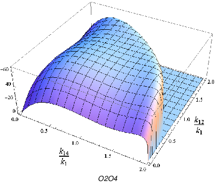
I ) Equilateral limit: it is defined by $k_{1}=k_{2}=k_{3}=k_{4}$ . We plot the trispectra $\mathcal{T}_{n}$ as functions of $k_{12}/k_{1}$ and $k_{14}/k_{1}$ in this configuration.

Specifically, in Fig. (3) we plot the SE trispectra and in Fig. (4,5) the CI trispectra including for comparison, in the last two plots, the two local-model trispectra.

In Fig. (3) we see that, at least qualitatively, in the equilateral configuration the SE-type shape-functions are similar to the corresponding $P(X,\phi)$ result¹⁰¹⁰ 10 At leading order in the $c_{s}\ll 1$ regime, the $P(X,\phi)$ model predicts the shapes we label as $O_{1}O_{1},O_{1}O_{3},O_{3}O_{3}.$ [25, 26]. One should also keep in mind that, as clear from the figure, here the overall sign of the form-factor can change.

Next, we move on (Fig. 4, 5) to the various CI-generated shape-functions in the same, equilateral, configuration. In this limit the significantly different shapes in comparison with $P(X,\phi)$ are generated by terms such as e.g. the $V_{8}$ -driven interaction in Fig. (4). The equilateral configuration plots (Fig. 4, 5) are indeed quite interesting: $P(X,\phi)$ models predict a simple plateau, which is what we obtain from terms such as the ones driven by the coefficients¹¹¹¹ 11 At leading order in the $c_{s}\ll 1$ regime, $P(X,\phi)$ produces only $V_{1}$ . $V_{1},V_{2},V_{3},V_{4},V_{6}$ and also from one local-type of trispectrum. On the other hand, this is clearly not the case for terms such as those proportional to $V_{5},V_{7},V_{8}$ , as well as the other local-type profile. These latter $V_{n}$ coefficients are then the most intriguing as they drive interactions which evidently have a quite different signature than any $P(X,\phi)$ realization.

It is important to keep in mind that what we have here is a $k$ -configuration dependent signature and that one would need to probe the trispectrum in its entirety in order to be on par with what is done for the bispectrum analysis. However, what we found is nevertheless a distinct signature, and, as we shall see, we will have some further noteworthy results in the double-squeezed configuration as well.

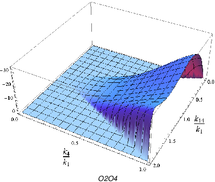
II ) Folded limit: $k_{12}=0$ . In this limit $k_{1}=k_{2}$ and $k_{3}=k_{4}$ . The trispectra are plotted as functions of $k_{4}/k_{1}$ and $k_{14}/k_{1}$ .

In Fig. (6) we plot the scalar-exchange trispectra and in Fig. (7,8) the contact-interaction trispectra including, in the last plot, the so-called Local2-type trispectra (Local1 is divergent in this limit).
Just as we saw for the SE equilateral configuration profiles, from the plots in Fig. (6) one can conclude that the patterns that emerge in $k$ -space for the folded configuration are very similar to those in the analysis of [25] for $P(X,\phi)$ models. As to the CI-generated plots in the folded configuration, we limit the graphical representations in the main text to the more illustrative cases. In this specific $k$ arrangement, it is again hard to see any qualitative difference with the work in [25].
It is also worth mentioning here that the $V_{8}$ regulated CI term does not contribute to any of the configurations in $II,III,IV$ and is therefore not plotted in the corresponding figures.

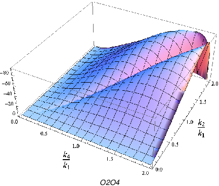
III ) Specialized planar limit: $k_{1}=k_{3}=k_{14}$ and the tetrahedron lies on a plane. One can solve for $k_{12}$ [25], to find $k_{12}=\left[k_{1}^{2}+\frac{k_{2}k_{4}}{2k_{1}^{2}}\left(k_{2}k_{4}+\sqrt{(4k_{1}^{2}-k_{2}^{2})(4k_{1}^{2}-k_{4}^{2})}\right)\right]^{\frac{1}{2}}$ . The trispectra are plotted as functions of $k_{2}/k_{1}$ and $k_{4}/k_{1}$ .

Following the presentation pattern of the previous two configurations, in Fig.(9) we have plotted some representative operators contribution to the scalar exchange diagram, namely the couples $\{O_{1}O_{1}\},\{O_{3}O_{3}\},\{O_{1}O_{3}\},\{O_{2}O_{4}\}$ , in the specialized planar configuration. In Fig. (10,11) we plot the contact-interaction trispectra including, as usual, the two local-model trispectra.

The same considerations we made for the folded configuration hold true for all the plots (SE as well as CI) in the specialized planar configuration. Upon a more quantitative analysis, one finds that the shape-functions are indeed analytically different from those in [25] (and from each other as well), but this fact in itself is not sufficient to claim a real significance for the difference. Indeed, in the case of qualitatively similar shape-functions a more detailed treatment, such as a shape scalar product analysis, would reveal small differences. On the other hand, for both the folded and the specialized planar configurations findings in this model we do not anticipate that the shape profiles differ from those of [25] to a sufficient degree so as to motivate such a detailed analysis.

IV ) Near the double-squeezed limit: $k_{3}=k_{4}=k_{12}$ and the tetrahedron is lying on a plane. In this limit $k_{2}$ [25] can be written in terms of the other variables as

k_{2}=\frac{1}{\sqrt{2}k_{4}}\sqrt{k_{1}^{2}(-k_{12}^{2}+k_{3}^{2}+k_{4}^{2})-k_{s1}^{2}k_{s2}^{2}+k_{12}^{2}k_{14}^{2}+k_{12}^{2}k_{4}^{2}+k_{14}^{2}k_{4}^{2}-k_{14}^{2}k_{3}^{2}-k_{4}^{4}+k_{3}^{2}k_{4}^{2}},

where the variables $k_{s1}$ and $k_{s2}$ are defined as

k_{s1}^{2}=2\sqrt{(k_{1}k_{4}+\mathbf{k}_{1}\cdot\mathbf{k}_{4})(k_{1}k_{4}-\mathbf{k}_{1}\cdot\mathbf{k}_{4})}\,\,,\qquad k_{s2}^{2}=2\sqrt{(k_{3}k_{4}+\mathbf{k}_{3}\cdot\mathbf{k}_{4})(k_{3}k_{4}-\mathbf{k}_{3}\cdot\mathbf{k}_{4})}\,\,.

The scalar products can be written as $\mathbf{k}_{1}\cdot\mathbf{k}_{4}=(k_{14}^{2}-k_{1}^{2}-k_{4}^{2})/2$ and $\mathbf{k}_{3}\cdot\mathbf{k}_{4}=(k_{12}^{2}-k_{3}^{2}-k_{4}^{2})/2$ . The trispectra $\mathcal{T}_{n}$ are plotted as functions of $k_{12}/k_{1}$ and $k_{14}/k_{1}$ but are this time further divided by $k_{1}k_{2}k_{3}k_{4}$ for enhancement in shape-comparison.

In Fig. (12) we report the plots of the scalar exchange trispectra while Fig. (13,14) reproduce the plots of the contact interaction trispectra and the two local-model trispectra.

Much like what we have seen in the equilateral configuration plots, we shall show below that the non-Gaussian characterization of Galileon inflation in the double-squeezed configuration pays off in that it allows one to distinguish between the Galileon model predictions and those of $P(X,\phi)$ models.

It is perhaps timely at this stage to remind the reader of an interesting fact concerning the double-squeezed configurations plots in the $P(X,\phi)$ case: one could say that, for these models, the double-squeezed configuration is actually “aware” of what sort of contribution, cubic or quartic, is sourcing any given shape-function. This is because in the $(k_{14}=1,k_{12}\rightarrow 0)$ (see e.g. Fig. 12) limit the shape-function is finite but non-zero for each SE-type contribution while it is always finite and precisely zero in the CI case.

One can imagine that, if it were somehow possible to probe observationally such a configuration, the degeneracy between third and fourth order interactions contribution to the trispectrum could in principle be removed. As we will see, this is not the case for Galileon inflation.

A quick look at Fig. (13) reveals how terms such as those CI-type interactions driven by the coefficient $V_{3},V_{7}$ do indeed have a well-defined and, most importantly, non-zero $k_{12}\rightarrow 0$ limit. This fact then reinstates in Galileon inflation the degeneracy which was lifted in [25] for $P(X,\phi)$ models. This latter characterization adds to the number of distinct features which the setup under scrutiny here does not share with the results of [15, 18, 25, 26].

In interpreting the significance of the various shape-functions one must exert some care in that we must not naively treat all the different interactions as necessarily independent. The bispectrum analysis for example reveals that, of the four initial cubic interactions, one can be field-redefined away [37] and one more would give (we verified this explicitly) a bispectrum contribution which is analytically identical to a specific linear combination of the contributions from the two remaining interactions (see the comments after Eq. ). We have excluded a number of cubic and quartic interactions terms from the trispectrum plots above because they generate shapes which are, at least qualitatively, indistinguishable from some of those we do plot. It is quite possible that, in doing so, we have restricted the remaining plotted shape-functions to be indeed all independent. It is possible, although very lengthy, to perform a complete “orthonormalization” of the interactions which contribute to the trispectrum. The difficulty lies in the fact that the $c_{n}$ coefficients in the interaction terms appear not just in linear combinations, but in quadratic and cubic powers.

There is however a simple way to see that the shapes we plotted are indeed easily (i.e. without fine tuning) generated in Galileon inflation and therefore their signatures represent a clear cut characterization of this inflationary model.

The fact that several interaction terms share a specific profile pattern, such as e.g. $V_{5},V_{7},...$ in the $k_{12}\rightarrow 0$ limit in the double-squeezed configuration, suggests that one may, easily and without fine tuning, arrange for such a shape or, in other words, identify a basis for the various interactions in such a way that one of the basis vector does posses such a behaviour.
So far we have been discussing the analytical equivalence between shapes. Although it is always possible to pin down analytically the differences among the various shape-functions, it is not realistic to use such an approach when dealing with actual observables. In this respect, it is quite instructive to look at what happens with the bispectrum. There is indeed a degree to which shape-functions are to be considered hardly distinguishable, when their-cross correlation is sufficiently high for a particular set of data ¹²¹² 12 In e.g. [78] the authors do not mark as “different” shapes which have an overlap which exceeds $>0.7$ .. We have been careful to stress here as distinctively different from each other only those shape-functions which, already at the qualitative level, clearly show a distinguishing profile.

4 Conclusions

This paper represents an attempt to navigate part of the landscape of inflationary models guided by observational as well as more formal criteria. The very recent success of the Planck mission has provided us with an improved sensitivity over non-Gaussian observables [5]; chief among them, the quantity $f_{NL}$ has been markedly constrained in three of its possible realizations, local, equilateral, orthogonal, and interesting tight constraints have been also put on some other specific non-standard inflationary models. We have detailed here our results on the study on the model of Galileon inflation, an inflationary mechanism that, for a large region of its parameters space, is easily compatible with Planck results, as far as the power spectrum and the bispectrum of curvature perturbations are concerned.

As soon as any model fits within the available observational bounds, it becomes crucial to characterize its properties so as to distinguish it from other realizations. This investigation in our case has been manifold. First we reported on the stability properties which, from a quantum field theory perspective, describe the Galileon inflation model [37]. We stressed second order equations of motion and non-renormalization properties that guarantee we are dealing with a predictive model.

We then went on to detail on the study of non-Gaussianities. The bispectrum analysis has already been performed [37] and, as it turns out, the shape-function typically peaks in the equilateral limit, just as it does for an array of inflationary models in the literature.

It was therefore essential for the model characterization to go further in perturbation theory and tackle the trispectrum of curvature fluctuations. Doing so pays off in terms of distinguishing this model from other well studied classes of inflationary theories such as $P(X,\phi)$ . Since the trispectrum momentum-dependence has too many variables to be plotted simultaneously, we opted for plots in a number of different momenta configurations which proves handy for comparison with other studies. In two of these configurations, equilateral and double-squeezed, several of the Galileon inflation interactions that contribute to the trispectrum generate a shape function which is strikingly different from its $P(X,\phi)$ counterpart. More specifically, for the most interesting interaction terms, the equilateral configuration shape-function is strongly different w.r.t. $P(X,\phi)$ models: it peaks where the $P(X,\phi)$ counterpart would have either local minima or a plateau. For the double-squeezed configuration one finds that often both the scalar-exchange and contact-interactions contributions are characterized by a profile that does not vanish in the $k_{12}\rightarrow 0$ limit. This is in clear contradistinction with what happens in $P(X,\phi)$ models for which there exists a clear cut third-vs-fourth order behaviour in that limit.

Having verified that the characterization of Galilean inflation through non-Gaussian observables enables one to identify distinct features which clearly distinguish this model from an entire class of inflationary theories, one should of course point to possible future sources of data that could actually enable such a comparison. Although the results to date of the Planck mission data analysis have been already implemented in the quest for determining the essential features of the most compelling inflationary model, more data is expected and the inclusion of polarization is bound to improve further the constraints on non-Gaussian observables. Further input on (primordial and otherwise) non-Gaussian characterizations of inflationary models is expected to originate from Large Scale Structure sources (see, e.g., [79, 80]) and possibly from future CMB polarization experiments (see, e.g., [81], [82] and [83]) Another important probe might well be 21cm cosmology [84, 85, 86, 87].

Within the realm of what one might call the Galilean approach to inflation, one should certainly count the work presented here, and, naturally, Ref. [37] (see also [88]) where the basis of the model were laid. This model represents a full theory endowed with an inflating background solution and whose stability rests on very firm ground. On the other hand, the appealing properties of Galileon theories have been employed also in a related setup in [38, 39] where the fluctuations of an inflating solution around an FLRW background have been equipped with Galilean symmetry. The control over the full theory is slightly relaxed in this latter case (background behaviour is assumed), more in the spirit of the pioneering work in [68]. The predictions in terms of non-Gaussian observables are not dissimilar within these two approaches. However, specific interaction terms behaviour presented here (e.g. what we call here the $V_{8}$ -driven interaction) has no corresponding interaction in the related approach [39] and might well provide a sufficiently distinguishing feature.

Having the predictions for both bispectrum and trispectrum at our disposal, one might well ask if, within the parameters space of the model (and in agreement with observations), there is room for a small-bispectrum vs large-trispectrum region in the parameter space of the model. As it turns out, this region does indeed exist and we refer the interested reader to an upcoming work of ours [89] for a detailed analysis. We stress already here that, because of the celebrated non-renormalization properties of Galileon inflation, whatever initial region we select in the parameter space, from there one can proceed safe in the knowledge that the dynamics will not evolve very far upon renormalization and therefore the initial choice will be, in this sense, stable.

Acknowledgments

The work of NB has been partially supported by the ASI/INAF Agreement I/072/09/0 for the Planck LFI Activity of Phase E2 and by the PRIN 2009 project “La Ricerca di non-Gaussianità Primordiale”. The work of ED was partially supported by DOE grant DE-FG02-94ER-40823 at the University of Minnesota. ED is happy to thank the CWRU Physics Department for friendly hospitality during several stages of this work. MF is very grateful to A.J. Tolley for many enlightening discussions. ED and MF would like to thank the Cosmology Group at the University of Padova, and INFN, Sezione di Padova, for support and for warm hospitality whilst parts of this work were being completed.

5 Appendix A. The leading order bispectrum

The result of [37] for the leading order (i.e. $\ddot{\phi}\sim\dot{H}\sim 0$ ) bispectrum is

$\displaystyle\langle\zeta(\mathbf{k}_{1})\zeta(\mathbf{k}_{2})\zeta(\mathbf{k}_{3})\rangle$	$\displaystyle=$	$\displaystyle-(2\pi)^{3}\delta^{(3)}(\mathbf{K_{b}}_{t})\frac{H^{9}}{4^{3}\dot{\phi}_{0}^{3}A^{3}}\frac{1}{c_{s}^{6}}\frac{1}{\Pi_{i}k_{i}^{3}}\Bigg[24\frac{\mathcal{O}_{1}+2Hc_{s}^{-2}\mathcal{O}_{2}}{H}\frac{\Pi_{i}k_{i}^{2}}{K_{b}^{3}}$
		$\displaystyle+4\frac{\mathcal{O}_{3}}{Hc_{s}^{2}}\frac{1}{K_{b}}\Bigg(k_{3}^{2}\mathbf{k}_{1}\cdot\mathbf{k}_{2}\left(1+\frac{K_{b}(k_{1}+k_{2})+2k_{1}k_{2}}{K_{b}^{2}}\right)$
		$\displaystyle+k_{1}^{2}\mathbf{k}_{2}\cdot\mathbf{k}_{3}\left(1+\frac{K_{b}(k_{2}+k_{3})+2k_{2}k_{3}}{K_{b}^{2}}\right)+k_{2}^{2}\mathbf{k}_{1}\cdot\mathbf{k}_{3}\left(1+\frac{K_{b}(k_{1}+k_{3})+2k_{1}k_{3}}{K_{b}^{2}}\right)\Bigg)$
		$\displaystyle+8\frac{\mathcal{O}_{4}}{c_{s}^{4}}\frac{1}{K_{b}}\left(1+\frac{3k_{1}k_{2}k_{3}+K_{b}\sum_{j<i}k_{i}k_{j}}{K_{b}^{3}}\right)\left(k_{1}^{2}\mathbf{k}_{2}\cdot\mathbf{k}_{3}+k_{2}^{2}\mathbf{k}_{1}\cdot\mathbf{k}_{3}+k_{3}^{2}\mathbf{k}_{1}\cdot\mathbf{k}_{2}\right)\Bigg],\qquad$

where $\mathbf{K_{b}}_{t}=\mathbf{k}_{1}+\mathbf{k}_{2}+\mathbf{k}_{3}$ and $K_{b}=k_{1}+k_{2}+k_{3}$ . One then defines the shapes in the usual way as:

\displaystyle Shape_{1}=(k_{1}k_{2}k_{3})^{2}\times\frac{1}{\Pi_{i}k_{i}^{3}}\frac{\Pi_{i}k_{i}^{2}}{K_{b}^{3}},

(24)

	$\displaystyle Shape_{2}$	$\displaystyle=$	$\displaystyle(k_{1}k_{2}k_{3})^{2}\times\frac{1}{\Pi_{i}k_{i}^{3}}\frac{1}{K_{b}}\Bigg(k_{3}^{2}\mathbf{k}_{1}\cdot\mathbf{k}_{2}\left(1+\frac{K_{b}(k_{1}+k_{2})+2k_{1}k_{2}}{K_{b}^{2}}\right)$		(25)
			$\displaystyle\qquad+k_{1}^{2}\mathbf{k}_{2}\cdot\mathbf{k}_{3}\left(1+\frac{K_{b}(k_{2}+k_{3})+2k_{2}k_{3}}{K_{b}^{2}}\right)+k_{2}^{2}\mathbf{k}_{1}\cdot\mathbf{k}_{3}\left(1+\frac{K_{b}(k_{1}+k_{3})+2k_{1}k_{3}}{K_{b}^{2}}\right)\Bigg),$		(25)

\displaystyle Shape_{3}

\displaystyle=

\displaystyle(k_{1}k_{2}k_{3})^{2}\times\frac{1}{\Pi_{i}k_{i}^{3}}\frac{1}{K_{b}}\left(1+\frac{3k_{1}k_{2}k_{3}+K_{b}\sum_{j<i}k_{i}k_{j}}{K_{b}^{3}}\right)\left(k_{1}^{2}\mathbf{k}_{2}\cdot\mathbf{k}_{3}+k_{2}^{2}\mathbf{k}_{1}\cdot\mathbf{k}_{3}+k_{3}^{2}\mathbf{k}_{1}\cdot\mathbf{k}_{2}\right).

It is a well-known fact that these three shapes are highly correlated with the equilateral template. Also one can show that $Shape_{3}=6\,Shape_{1}+Shape_{2}$ .

6 Appendix B. Contact interaction trispectra

For the computation of the trispectrum diagrams, we use the leading-order in slow-roll mode function solution for $\delta\phi$

u(\tau,k)=\frac{N}{k^{3/2}}\left(1+ikc_{s}\tau\right)e^{-ikc_{s}\tau},

(27)

where the normalization factor is $N\equiv H/(2\sqrt{Ac_{s}^{3}})$ .

We expand $\delta\phi(\tau,\mathbf{k})=u(\tau,k)a(\mathbf{k})+u^{*}(\tau,k)a^{\dagger}(-\mathbf{k})$ with the standard commutation relations $\left[a(\mathbf{k}_{1}),a^{\dagger}(\mathbf{k}_{2})\right]=(2\pi)^{3}\delta^{(3)}(\mathbf{k}_{1}-\mathbf{k}_{2})$ and use

	$\displaystyle FPF$	$\displaystyle\equiv$	$\displaystyle\langle\Omega\|\delta\phi(0,\mathbf{k}_{1})\delta\phi(0,\mathbf{k}_{2})\delta\phi(0,\mathbf{k}_{3})\delta\phi(0,\mathbf{k}_{4})\|\Omega\rangle$		(28)
		$\displaystyle=$	$\displaystyle-i\int_{-\infty}^{0}dt\langle 0\|\!\!\left[\delta\phi(0,\mathbf{k}_{1})\delta\phi(0,\mathbf{k}_{2})\delta\phi(0,\mathbf{k}_{3})\delta\phi(0,\mathbf{k}_{4}),H^{(4)}_{I}(t)\right]\!\!\|0\rangle,$		(28)

where $H_{I}=\int d^{3}x\mathcal{H}_{I}$ is given at fourth order by (13). Then for each of the individual terms in (13) we obtain

\displaystyle FPF_{V_{1}}

\displaystyle=

\displaystyle-(2\pi)^{3}\delta^{(3)}(\mathbf{K}_{t})\frac{4N^{8}}{(k_{1}k_{2}k_{3}k_{4})^{3}}12V_{1}c_{s}^{3}\frac{(k_{1}k_{2}k_{3}k_{4})^{2}}{K^{5}}+23\mathrm{\,perms.},

(29)

\displaystyle FPF_{V_{2}}

\displaystyle=

\displaystyle-(2\pi)^{3}\delta^{(3)}(\mathbf{K}_{t})\frac{4N^{8}}{(k_{1}k_{2}k_{3}k_{4})^{3}}12V_{2}Hc_{s}\frac{(k_{1}k_{2}k_{3}k_{4})^{2}}{K^{5}}\left(1+5\frac{k_{4}}{K}\right)+23\mathrm{\,perms.},

(30)

	$\displaystyle FPF_{V_{3}}$	$\displaystyle=$	$\displaystyle-(2\pi)^{3}\delta^{(3)}(\mathbf{K}_{t})\frac{4N^{8}}{(k_{1}k_{2}k_{3}k_{4})^{3}}V_{3}c_{s}\frac{k_{1}^{2}k_{2}^{2}\mathbf{k}_{3}\cdot\mathbf{k}_{4}}{K^{5}}\left(K^{2}+3K\left(k_{3}+k_{4}\right)+12k_{3}k_{4}\right)$		(31)
		$\displaystyle+$	$\displaystyle 23\mathrm{\,perms.},$		(31)

	$\displaystyle FPF_{V_{4}}$	$\displaystyle=$	$\displaystyle-(2\pi)^{3}\delta^{(3)}(\mathbf{K}_{t})\frac{4N^{8}}{(k_{1}k_{2}k_{3}k_{4})^{3}}\frac{12V_{4}H^{2}}{c_{s}}\frac{(k_{1}k_{2}k_{3}k_{4})^{2}}{K^{5}}\left(1+\frac{5}{K}\left(k_{3}+k_{4}\right)+\frac{30k_{3}k_{4}}{K^{2}}\right)$		(32)
		$\displaystyle+$	$\displaystyle 23\mathrm{\,perms.},$		(32)

	$\displaystyle FPF_{V_{5}}$	$\displaystyle=$	$\displaystyle-(2\pi)^{3}\delta^{(3)}(\mathbf{K}_{t})\frac{4N^{8}}{(k_{1}k_{2}k_{3}k_{4})^{3}}\frac{12V_{5}H^{2}}{c_{s}}\frac{k_{1}^{2}k_{2}^{2}(\mathbf{k}_{3}\cdot\mathbf{k}_{4})^{2}}{K^{5}}\left(1+\frac{5}{K}\left(k_{3}+k_{4}\right)+\frac{30k_{3}k_{4}}{K^{2}}\right)$		(33)
		$\displaystyle+$	$\displaystyle 23\mathrm{\,perms.},$		(33)

	$\displaystyle FPF_{V_{6}}$	$\displaystyle=$	$\displaystyle-(2\pi)^{3}\delta^{(3)}(\mathbf{K}_{t})\frac{4N^{8}}{(k_{1}k_{2}k_{3}k_{4})^{3}}\frac{V_{6}H}{c_{s}}\frac{k_{1}^{2}k_{4}^{2}\mathbf{k}_{2}\cdot\mathbf{k}_{3}}{K^{5}}\Big(4K^{2}-3k_{1}K+12\left(k_{2}k_{3}+k_{2}k_{4}+k_{3}k_{4}\right)$		(34)
			$\displaystyle+60\frac{k_{2}k_{3}k_{4}}{K}\Big)+23\mathrm{\,perms.},$		(34)

	$\displaystyle FPF_{V_{7}}$	$\displaystyle=$	$\displaystyle-(2\pi)^{3}\delta^{(3)}(\mathbf{K}_{t})\frac{4N^{8}}{(k_{1}k_{2}k_{3}k_{4})^{3}}\frac{V_{7}}{c_{s}}\frac{\mathbf{k}_{1}\cdot\mathbf{k}_{2}\mathbf{k}_{3}\cdot\mathbf{k}_{4}}{K^{5}}\Big(K^{4}+K^{2}\sum_{i=1}^{4}\sum_{j>i}^{4}k_{i}k_{j}$		(35)
		$\displaystyle+$	$\displaystyle 3K\sum_{l=1}^{4}\sum_{m>l}^{4}\sum_{n>m}^{4}k_{l}k_{m}k_{n}+12k_{1}k_{2}k_{3}k_{4}\Big)+23\mathrm{\,perms.},$		(35)

	$\displaystyle FPF_{V_{8}}$	$\displaystyle=$	$\displaystyle(2\pi)^{3}\delta^{(3)}(\mathbf{K}_{t})\frac{4N^{8}}{(k_{1}k_{2}k_{3}k_{4})^{3}}\frac{V_{8}H^{2}}{c_{s}^{3}}\frac{\mathbf{k}_{1}\cdot\mathbf{k}_{2}((\mathbf{k}_{3}\cdot\mathbf{k}_{4})^{2}-k_{3}^{2}k_{4}^{2})}{K^{5}}$		(36)
			$\displaystyle\times\left(4K^{2}+12\sum_{i=1}^{4}\sum_{j>i}^{4}k_{i}k_{j}+\frac{60}{K}\sum_{l=1}^{4}\sum_{m>l}^{4}\sum_{n>m}^{4}k_{l}k_{m}k_{n}+360\frac{k_{1}k_{2}k_{3}k_{4}}{K^{2}}\right)+23\mathrm{\,perms.},$		(36)

where $K=k_{1}+k_{2}+k_{3}+k_{4}$ and $\mathbf{K}_{t}=\mathbf{k}_{1}+\mathbf{k}_{2}+\mathbf{k}_{3}+\mathbf{k}_{4}$ .

Note that not all the CI contributions to the trispectrum are independent, indeed, after some manipulations one finds:

\displaystyle FPF_{V_{2}}|_{V_{2}=1}=\frac{9H}{4c_{s}^{2}}FPF_{V_{1}}|_{V_{1}=1},\qquad FPF_{V_{6}}|_{V_{6}=1}=\frac{3H}{4c_{s}^{4}}FPF_{V_{1}}|_{V_{1}=1}+\frac{5H}{2c_{s}^{2}}FPF_{V_{3}}|_{V_{3}=1}.

7 Appendix C. Scalar exchange trispectra

	$\mathcal{O}_{1}^{R}$	$\mathcal{O}_{2}^{R}$	$\mathcal{O}_{3}^{R}$	$\mathcal{O}_{4}^{R}$
$\mathcal{O}_{1}^{L}$	$\mathcal{F}_{1}$	$\mathcal{F}_{5}$	$\mathcal{F}_{3}$	$\mathcal{F}_{7}$
$\mathcal{O}_{2}^{L}$	$\mathcal{F}_{6}$	$\mathcal{F}_{9}$	$\mathcal{F}_{10}$	$\mathcal{F}_{12}$
$\mathcal{O}_{3}^{L}$	$\mathcal{F}_{4}$	$\mathcal{F}_{11}$	$\mathcal{F}_{2}$	$\mathcal{F}_{14}$
$\mathcal{O}_{4}^{L}$	$\mathcal{F}_{8}$	$\mathcal{F}_{13}$	$\mathcal{F}_{15}$	$\mathcal{F}_{16}$

Table 1: Rules to decide which

\mathcal{F}_{i}

to use when writing the contribution of a certain diagram according to the diagrammatic rules of [27]. For example, if the lhs vertex of the diagram is the vertex proportional to

\mathcal{O}_{3}

and the rhs vertex is the vertex proportional to

\mathcal{O}_{4}

then the functions to use is

\mathcal{F}_{14}

For the SE trispectrum contribution, one employs the following:

	$\displaystyle FPF^{SE}$	$\displaystyle\equiv$	$\displaystyle\langle\Omega\|\delta\phi(0,k_{1})\delta\phi(0,k_{2})\delta\phi(0,k_{3})\delta\phi(0,k_{4})\|\Omega\rangle$
		$\displaystyle=$	$\displaystyle-\int_{-\infty}^{0}dt\int_{-\infty}^{t}d\tilde{t}\langle 0\|\Big[\big[\delta\phi(0,k_{1})\delta\phi(0,k_{2})\delta\phi(0,k_{3})\delta\phi(0,k_{4}),H_{I}^{(3)}(t)\big],H_{I}^{(3)}(\tilde{t})\Big]\|0\rangle.$

The different trispecta coming from the different vertices can be written as (using the diagrammatic approach rules described in [27] and Table 1)

$\displaystyle FPF^{SE}_{\mathcal{O}_{1}\mathcal{O}_{2}}$	$\displaystyle=$	$\displaystyle-2(2\pi)^{3}\delta^{(3)}(\mathbf{K}_{t})\frac{N^{4}}{(k_{1}k_{2}k_{3}k_{4})^{\frac{3}{2}}}\mathcal{O}_{1}\mathcal{O}_{2}$	(39)
		$\displaystyle\times\Big[-3\mathbf{k}_{12}\cdot\mathbf{k}_{12}\Big(\mathcal{F}_{5}(k_{1},k_{2},-k_{12},k_{3},k_{4},k_{12})-\mathcal{F}_{5}(-k_{1},-k_{2},-k_{12},k_{3},k_{4},k_{12})\Big)$
		$\displaystyle\quad\;\,-6k_{4}^{2}\Big(\mathcal{F}_{5}(k_{1},k_{2},-k_{12},k_{3},k_{12},k_{4})-\mathcal{F}_{5}(-k_{1},-k_{2},-k_{12},k_{3},k_{12},k_{4})\Big)$
		$\displaystyle\quad\;\,-3\mathbf{k}_{12}\cdot\mathbf{k}_{12}\Big(\mathcal{F}_{6}(k_{1},k_{2},-k_{12},k_{3},k_{4},k_{12})-\mathcal{F}_{6}(-k_{1},-k_{2},-k_{12},k_{3},k_{4},k_{12})\Big)$
		$\displaystyle\quad\;\,-6k_{2}^{2}\Big(\mathcal{F}_{6}(k_{1},-k_{12},k_{2},k_{3},k_{4},k_{12})-\mathcal{F}_{6}(-k_{1},-k_{12},-k_{2},k_{3},k_{4},k_{12})\Big)\Big]$
		$\displaystyle+23\,\mathrm{perms.\,of\,\{k_{1},k_{2},k_{3},k_{4}\}},$

$\displaystyle FPF^{SE}_{\mathcal{O}_{1}\mathcal{O}_{4}}$	$\displaystyle=$	$\displaystyle-2(2\pi)^{3}\delta^{(3)}(\mathbf{K}_{t})\frac{N^{4}}{(k_{1}k_{2}k_{3}k_{4})^{\frac{3}{2}}}\mathcal{O}_{1}\mathcal{O}_{4}$	(40)
		$\displaystyle\times\Big[\left(3k_{12}^{2}\mathbf{k}_{3}\cdot\mathbf{k}_{4}+6k_{4}^{2}\mathbf{k}_{3}\cdot\mathbf{k}_{12}\right)\Big(\mathcal{F}_{7}(k_{1},k_{2},-k_{12},k_{3},k_{4},k_{12})$
		$\displaystyle-\mathcal{F}_{7}(-k_{1},-k_{2},-k_{12},k_{3},k_{4},k_{12})\Big)$
		$\displaystyle\quad\;\,+\left(3k_{12}^{2}\mathbf{k}_{1}\cdot\mathbf{k}_{2}-6k_{2}^{2}\mathbf{k}_{1}\cdot\mathbf{k}_{12}\right)\Big(\mathcal{F}_{8}(k_{1},k_{2},-k_{12},k_{3},k_{4},k_{12})$
		$\displaystyle-\mathcal{F}_{8}(-k_{1},-k_{2},-k_{12},k_{3},k_{4},k_{12})\Big)\Big]+23\,\mathrm{perms.\,of\,\{k_{1},k_{2},k_{3},k_{4}\}},$

$\displaystyle FPF^{SE}_{\mathcal{O}_{2}\mathcal{O}_{3}}$	$\displaystyle=$	$\displaystyle-2(2\pi)^{3}\delta^{(3)}(\mathbf{K}_{t})\frac{N^{4}}{(k_{1}k_{2}k_{3}k_{4})^{\frac{3}{2}}}\mathcal{O}_{2}\mathcal{O}_{3}$	(41)
		$\displaystyle\times\Big[k_{12}^{2}\mathbf{k}_{3}\cdot\mathbf{k}_{4}\Big(\mathcal{F}_{10}(k_{1},k_{2},-k_{12},k_{12},k_{3},k_{4})-\mathcal{F}_{10}(-k_{1},-k_{2},-k_{12},k_{12},k_{3},k_{4})\Big)$
		$\displaystyle\quad\;\,+2k_{12}^{2}\mathbf{k}_{4}\cdot\mathbf{k}_{12}\Big(\mathcal{F}_{10}(k_{1},k_{2},-k_{12},k_{3},k_{4},k_{12})-\mathcal{F}_{10}(-k_{1},-k_{2},-k_{12},k_{3},k_{4},k_{12})\Big)$
		$\displaystyle\quad\;\,+2k_{2}^{2}\mathbf{k}_{3}\cdot\mathbf{k}_{4}\Big(\mathcal{F}_{10}(k_{1},-k_{12},k_{2},k_{12},k_{3},k_{4})-\mathcal{F}_{10}(-k_{1},-k_{12},-k_{2},k_{12},k_{3},k_{4})\Big)$
		$\displaystyle\quad\;\,+4k_{2}^{2}\mathbf{k}_{4}\cdot\mathbf{k}_{12}\Big(\mathcal{F}_{10}(k_{1},-k_{12},k_{2},k_{3},k_{4},k_{12})-\mathcal{F}_{10}(-k_{1},-k_{12},-k_{2},k_{3},k_{4},k_{12})\Big)$
		$\displaystyle\quad\;\,+k_{12}^{2}\mathbf{k}_{1}\cdot\mathbf{k}_{2}\Big(\mathcal{F}_{11}(-k_{12},k_{1},k_{2},k_{3},k_{4},k_{12})-\mathcal{F}_{11}(-k_{12},-k_{1},-k_{2},k_{3},k_{4},k_{12})\Big)$
		$\displaystyle\quad\;\,+2k_{4}^{2}\mathbf{k}_{1}\cdot\mathbf{k}_{2}\Big(\mathcal{F}_{11}(-k_{12},k_{1},k_{2},k_{3},k_{12},k_{4})-\mathcal{F}_{11}(-k_{12},-k_{1},-k_{2},k_{3},k_{12},k_{4})\Big)$
		$\displaystyle\quad\;\,-2k_{12}^{2}\mathbf{k}_{2}\cdot\mathbf{k}_{12}\Big(\mathcal{F}_{11}(k_{1},k_{2},-k_{12},k_{3},k_{4},k_{12})-\mathcal{F}_{11}(-k_{1},-k_{2},-k_{12},k_{3},k_{4},k_{12})\Big)$
		$\displaystyle\quad\;\,-4k_{4}^{2}\mathbf{k}_{2}\cdot\mathbf{k}_{12}\Big(\mathcal{F}_{11}(k_{1},k_{2},-k_{12},k_{3},k_{12},k_{4})-\mathcal{F}_{11}(-k_{1},-k_{2},-k_{12},k_{3},k_{12},k_{4})\Big)\Big]$
		$\displaystyle+23\,\mathrm{perms.\,of\,\{k_{1},k_{2},k_{3},k_{4}\}},$

$\displaystyle FPF^{SE}_{\mathcal{O}_{2}\mathcal{O}_{4}}$	$\displaystyle=$	$\displaystyle-2(2\pi)^{3}\delta^{(3)}(\mathbf{K}_{t})\frac{N^{4}}{(k_{1}k_{2}k_{3}k_{4})^{\frac{3}{2}}}\mathcal{O}_{2}\mathcal{O}_{4}$	(42)
		$\displaystyle\times\Big[-k_{12}^{2}\left(k_{12}^{2}\mathbf{k}_{3}\cdot\mathbf{k}_{4}+2k_{4}^{2}\mathbf{k}_{3}\cdot\mathbf{k}_{12}\right)\Big(\mathcal{F}_{12}(k_{1},k_{2},-k_{12},k_{3},k_{4},k_{12})$
		$\displaystyle-\mathcal{F}_{12}(-k_{1},-k_{2},-k_{12},k_{3},k_{4},k_{12})\Big)$
		$\displaystyle\quad\;\,-2k_{2}^{2}\left(k_{12}^{2}\mathbf{k}_{3}\cdot\mathbf{k}_{4}+2k_{4}^{2}\mathbf{k}_{3}\cdot\mathbf{k}_{12}\right)\Big(\mathcal{F}_{12}(k_{1},-k_{12},k_{2},k_{3},k_{4},k_{12})$
		$\displaystyle-\mathcal{F}_{12}(-k_{1},-k_{12},-k_{2},k_{3},k_{4},k_{12})\Big)$
		$\displaystyle\quad\;\,-k_{12}^{2}\left(k_{12}^{2}\mathbf{k}_{1}\cdot\mathbf{k}_{2}-2k_{2}^{2}\mathbf{k}_{1}\cdot\mathbf{k}_{12}\right)\Big(\mathcal{F}_{13}(k_{1},k_{2},-k_{12},k_{3},k_{4},k_{12})$
		$\displaystyle-\mathcal{F}_{13}(-k_{1},-k_{2},-k_{12},k_{3},k_{4},k_{12})\Big)$
		$\displaystyle\quad\;\,-2k_{4}^{2}\left(k_{12}^{2}\mathbf{k}_{1}\cdot\mathbf{k}_{2}-2k_{2}^{2}\mathbf{k}_{1}\cdot\mathbf{k}_{12}\right)\Big(\mathcal{F}_{13}(k_{1},k_{2},-k_{12},k_{3},k_{12},k_{4})$
		$\displaystyle-\mathcal{F}_{13}(-k_{1},-k_{2},-k_{12},k_{3},k_{12},k_{4})\Big)\Big]+23\,\mathrm{perms.\,of\,\{k_{1},k_{2},k_{3},k_{4}\}},$

$\displaystyle FPF^{SE}_{\mathcal{O}_{3}\mathcal{O}_{4}}$	$\displaystyle=$	$\displaystyle-2(2\pi)^{3}\delta^{(3)}(\mathbf{K}_{t})\frac{N^{4}}{(k_{1}k_{2}k_{3}k_{4})^{\frac{3}{2}}}\mathcal{O}_{3}\mathcal{O}_{4}$	(43)
		$\displaystyle\times\Big[-\mathbf{k}_{1}\cdot\mathbf{k}_{2}\left(k_{12}^{2}\mathbf{k}_{3}\cdot\mathbf{k}_{4}+2k_{4}^{2}\mathbf{k}_{3}\cdot\mathbf{k}_{12}\right)\Big(\mathcal{F}_{14}(-k_{12},k_{1},k_{2},k_{3},k_{4},k_{12})$
		$\displaystyle-\mathcal{F}_{14}(-k_{12},-k_{1},-k_{2},k_{3},k_{4},k_{12})\Big)$
		$\displaystyle\quad\;\,+2\mathbf{k}_{2}\cdot\mathbf{k}_{12}\left(k_{12}^{2}\mathbf{k}_{3}\cdot\mathbf{k}_{4}+2k_{4}^{2}\mathbf{k}_{3}\cdot\mathbf{k}_{12}\right)\Big(\mathcal{F}_{14}(k_{1},k_{2},-k_{12},k_{3},k_{4},k_{12})$
		$\displaystyle-\mathcal{F}_{14}(-k_{1},-k_{2},-k_{12},k_{3},k_{4},k_{12})\Big)$
		$\displaystyle\quad\;\,-\mathbf{k}_{3}\cdot\mathbf{k}_{4}\left(k_{12}^{2}\mathbf{k}_{1}\cdot\mathbf{k}_{2}-2k_{2}^{2}\mathbf{k}_{1}\cdot\mathbf{k}_{12}\right)\Big(\mathcal{F}_{15}(k_{1},k_{2},-k_{12},k_{12},k_{3},k_{4})$
		$\displaystyle-\mathcal{F}_{15}(-k_{1},-k_{2},-k_{12},k_{12},k_{3},k_{4})\Big)$
		$\displaystyle\quad\;\,-2\mathbf{k}_{4}\cdot\mathbf{k}_{12}\left(k_{12}^{2}\mathbf{k}_{1}\cdot\mathbf{k}_{2}-2k_{2}^{2}\mathbf{k}_{1}\cdot\mathbf{k}_{12}\right)\Big(\mathcal{F}_{15}(k_{1},k_{2},-k_{12},k_{3},k_{4},k_{12})$
		$\displaystyle-\mathcal{F}_{15}(-k_{1},-k_{2},-k_{12},k_{3},k_{4},k_{12})\Big)\Big]+23\,\mathrm{perms.\,of\,\{k_{1},k_{2},k_{3},k_{4}\}},$

$\displaystyle FPF^{SE}_{\mathcal{O}_{2}\mathcal{O}_{2}}$	$\displaystyle=$	$\displaystyle-2(2\pi)^{3}\delta^{(3)}(\mathbf{K}_{t})\frac{N^{4}}{(k_{1}k_{2}k_{3}k_{4})^{\frac{3}{2}}}\mathcal{O}_{2}^{2}$	(44)
		$\displaystyle\times\Big[k_{12}^{4}\Big(\mathcal{F}_{9}(k_{1},k_{2},-k_{12},k_{3},k_{4},k_{12})-\mathcal{F}_{9}(-k_{1},-k_{2},-k_{12},k_{3},k_{4},k_{12})\Big)$
		$\displaystyle\quad\;\,+2k_{4}^{2}k_{12}^{2}\Big(\mathcal{F}_{9}(k_{1},k_{2},-k_{12},k_{3},k_{12},k_{4})-\mathcal{F}_{9}(-k_{1},-k_{2},-k_{12},k_{3},k_{12},k_{4})\Big)$
		$\displaystyle\quad\;\,+2k_{2}^{2}k_{12}^{2}\Big(\mathcal{F}_{9}(k_{1},-k_{12},k_{2},k_{3},k_{4},k_{12})-\mathcal{F}_{9}(-k_{1},-k_{12},-k_{2},k_{3},k_{4},k_{12})\Big)$
		$\displaystyle\quad\;\,+4k_{2}^{2}k_{4}^{2}\Big(\mathcal{F}_{9}(k_{1},-k_{12},k_{2},k_{3},k_{12},k_{4})-\mathcal{F}_{9}(-k_{1},-k_{12},-k_{2},k_{3},k_{12},k_{4})\Big)\Big]$
		$\displaystyle+23\,\mathrm{perms.\,of\,\{k_{1},k_{2},k_{3},k_{4}\}},$

$\displaystyle FPF^{SE}_{\mathcal{O}_{4}\mathcal{O}_{4}}$	$\displaystyle=$	$\displaystyle-2(2\pi)^{3}\delta^{(3)}(\mathbf{K}_{t})\frac{N^{4}}{(k_{1}k_{2}k_{3}k_{4})^{\frac{3}{2}}}\mathcal{O}_{4}^{2}$	(45)
		$\displaystyle\times\Big(k_{12}^{4}(\mathbf{k}_{1}\cdot\mathbf{k}_{2})(\mathbf{k}_{3}\cdot\mathbf{k}_{4})+2k_{4}^{2}k_{12}^{2}(\mathbf{k}_{1}\cdot\mathbf{k}_{2})(\mathbf{k}_{3}\cdot\mathbf{k}_{12})-2k_{2}^{2}k_{12}^{2}(\mathbf{k}_{1}\cdot\mathbf{k}_{12})(\mathbf{k}_{3}\cdot\mathbf{k}_{4})$
		$\displaystyle-4k_{2}^{2}k_{4}^{2}(\mathbf{k}_{1}\cdot\mathbf{k}_{12})(\mathbf{k}_{3}\cdot\mathbf{k}_{12})\Big)\Big(\mathcal{F}_{16}(k_{1},k_{2},-k_{12},k_{3},k_{4},k_{12})$
		$\displaystyle-\mathcal{F}_{16}(-k_{1},-k_{2},-k_{12},k_{3},k_{4},k_{12})\Big)+23\,\mathrm{perms.\,of\,\{k_{1},k_{2},k_{3},k_{4}\}},$

	$\displaystyle FPF^{SE}_{\mathcal{O}_{1}\mathcal{O}_{1}}$	$\displaystyle=$	$\displaystyle-2(2\pi)^{3}\delta^{(3)}(\mathbf{K}_{t})\frac{N^{4}}{(k_{1}k_{2}k_{3}k_{4})^{\frac{3}{2}}}9\mathcal{O}_{1}^{2}\Big(\mathcal{F}_{1}(k_{1},k_{2},-k_{12},k_{3},k_{4},k_{12})$		(46)
			$\displaystyle-\mathcal{F}_{1}(-k_{1},-k_{2},-k_{12},k_{3},k_{4},k_{12})\Big)+23\,\mathrm{perms.\,of\,\{k_{1},k_{2},k_{3},k_{4}\}},$		(46)

$\displaystyle FPF^{SE}_{\mathcal{O}_{3}\mathcal{O}_{3}}$	$\displaystyle=$	$\displaystyle-2(2\pi)^{3}\delta^{(3)}(\mathbf{K}_{t})\frac{N^{4}}{(k_{1}k_{2}k_{3}k_{4})^{\frac{3}{2}}}\mathcal{O}_{3}^{2}$	(47)
		$\displaystyle\times\Big[(\mathbf{k}_{1}\cdot\mathbf{k}_{2})(\mathbf{k}_{3}\cdot\mathbf{k}_{4})\Big(\mathcal{F}_{2}(-k_{12},k_{1},k_{2},k_{12},k_{3},k_{4})-\mathcal{F}_{2}(-k_{12},-k_{1},-k_{2},k_{12},k_{3},k_{4})\Big)$
		$\displaystyle\quad\;\,+2(\mathbf{k}_{1}\cdot\mathbf{k}_{2})(\mathbf{k}_{4}\cdot\mathbf{k}_{12})\Big(\mathcal{F}_{2}(-k_{12},k_{1},k_{2},k_{3},k_{4},k_{12})-\mathcal{F}_{2}(-k_{12},-k_{1},-k_{2},k_{3},k_{4},k_{12})\Big)$
		$\displaystyle\quad\;\,-2(\mathbf{k}_{2}\cdot\mathbf{k}_{12})(\mathbf{k}_{3}\cdot\mathbf{k}_{4})\Big(\mathcal{F}_{2}(k_{1},k_{2},-k_{12},k_{12},k_{3},k_{4})-\mathcal{F}_{2}(-k_{1},-k_{2},-k_{12},k_{12},k_{3},k_{4})\Big)$
		$\displaystyle\quad\;\,-4(\mathbf{k}_{2}\cdot\mathbf{k}_{12})(\mathbf{k}_{4}\cdot\mathbf{k}_{12})\Big(\mathcal{F}_{2}(k_{1},k_{2},-k_{12},k_{3},k_{4},k_{12})-\mathcal{F}_{2}(-k_{1},-k_{2},-k_{12},k_{3},k_{4},k_{12})\Big)\Big]$
		$\displaystyle+23\,\mathrm{perms.\,of\,\{k_{1},k_{2},k_{3},k_{4}\}},$

$\displaystyle FPF^{SE}_{\mathcal{O}_{1}\mathcal{O}_{3}}$	$\displaystyle=$	$\displaystyle-2(2\pi)^{3}\delta^{(3)}(\mathbf{K}_{t})\frac{N^{4}}{(k_{1}k_{2}k_{3}k_{4})^{\frac{3}{2}}}\mathcal{O}_{1}\mathcal{O}_{3}$	(48)
		$\displaystyle\times\Big[-3\mathbf{k}_{3}\cdot\mathbf{k}_{4}\Big(\mathcal{F}_{3}(k_{1},k_{2},-k_{12},k_{12},k_{3},k_{4})-\mathcal{F}_{3}(-k_{1},-k_{2},-k_{12},k_{12},k_{3},k_{4})\Big)$
		$\displaystyle\quad\;\,-6\mathbf{k}_{4}\cdot\mathbf{k}_{12}\Big(\mathcal{F}_{3}(k_{1},k_{2},-k_{12},k_{3},k_{4},k_{12})-\mathcal{F}_{3}(-k_{1},-k_{2},-k_{12},k_{3},k_{4},k_{12})\Big)$
		$\displaystyle\quad\;\,-3\mathbf{k}_{1}\cdot\mathbf{k}_{2}\Big(\mathcal{F}_{4}(-k_{12},k_{1},k_{2},k_{3},k_{4},k_{12})-\mathcal{F}_{4}(-k_{12},-k_{1},-k_{2},k_{3},k_{4},k_{12})\Big)$
		$\displaystyle\quad\;\,+6\mathbf{k}_{2}\cdot\mathbf{k}_{12}\Big(\mathcal{F}_{4}(k_{1},k_{2},-k_{12},k_{3},k_{4},k_{12})-\mathcal{F}_{4}(-k_{1},-k_{2},-k_{12},k_{3},k_{4},k_{12})\Big)\Big]$
		$\displaystyle+23\,\mathrm{perms.\,of\,\{k_{1},k_{2},k_{3},k_{4}\}},$

where the last three equations are the ones that appear in the $P(X,\phi)$ model and $k_{12}=|\mathbf{k}_{12}|=|\mathbf{k}_{1}+\mathbf{k}_{2}|$ . Similarly we define $k_{ab}$ as $k_{ab}=|\mathbf{k}_{ab}|=|\mathbf{k}_{a}+\mathbf{k}_{b}|$ , where $\mathbf{k}_{a}$ and $\mathbf{k}_{b}$ represent any of the four momentum vectors $\mathbf{k}_{1}$ , $\mathbf{k}_{2}$ , $\mathbf{k}_{3}$ and $\mathbf{k}_{4}$ . Momentum conservation implies $k_{12}=k_{34}$ , $k_{13}=k_{24}$ and $k_{14}=k_{23}$ .

Using the modified mode function $U(\tau,k)$ defined as ¹³¹³ 13 If the sign of the argument $k$ is positive then $U$ is equal to the mode function, if the sign is negative then $U$ is equal to the complex conjugate of the mode function.

U(\tau,k)\equiv\frac{N}{|k|^{3/2}}(1+ikc_{s}\tau)e^{-ikc_{s}\tau},

(49)

we define 16 $\mathcal{F}_{i}(k_{1},k_{2},k_{3},k_{4},k_{5},k_{6})$ functions as

	$\displaystyle\mathcal{F}_{1}(k_{1},...,k_{6})$	$\displaystyle=$	$\displaystyle\int^{0}_{-\infty}d\tau a(\tau)\int^{\tau}_{-\infty}d\tilde{\tau}a(\tilde{\tau})U^{^{\prime}}(\tau,k_{1})U^{^{\prime}}(\tau,k_{2})U^{^{\prime}}(\tau,k_{3})U^{^{\prime}}(\tilde{\tau},k_{4})U^{^{\prime}}(\tilde{\tau},k_{5})U^{^{\prime}}(\tilde{\tau},k_{6})$		(50)
		$\displaystyle=$	$\displaystyle-4\frac{N^{6}c_{s}^{6}}{H^{2}}\|k_{1}\cdots k_{6}\|^{\frac{1}{2}}\frac{1}{\mathcal{A}^{3}\mathcal{C}^{3}}\left(1+3\frac{\mathcal{A}}{\mathcal{C}}+6\frac{\mathcal{A}^{2}}{\mathcal{C}^{2}}\right),$		(50)

$\displaystyle\mathcal{F}_{2}(k_{1},...,k_{6})$	$\displaystyle=$	$\displaystyle\int^{0}_{-\infty}d\tau a(\tau)\int^{\tau}_{-\infty}d\tilde{\tau}a(\tilde{\tau})U^{^{\prime}}(\tau,k_{1})U^{}(\tau,k_{2})U^{}(\tau,k_{3})U^{^{\prime}}(\tilde{\tau},k_{4})U^{}(\tilde{\tau},k_{5})U^{}(\tilde{\tau},k_{6})$	(51)
	$\displaystyle=$	$\displaystyle-\frac{N^{6}c_{s}^{2}}{H^{2}}\frac{\|k_{1}k_{4}\|^{\frac{1}{2}}}{\|k_{2}k_{3}k_{5}k_{6}\|^{\frac{3}{2}}}\frac{1}{\mathcal{A}\mathcal{C}}\bigg[1+\frac{k_{5}+k_{6}}{\mathcal{A}}+2\frac{k_{5}k_{6}}{\mathcal{A}^{2}}$
		$\displaystyle+\frac{1}{\mathcal{C}}\left(k_{2}+k_{3}+k_{5}+k_{6}+\frac{1}{\mathcal{A}}\left(\left(k_{2}+k_{3}\right)\left(k_{5}+k_{6}\right)+2k_{5}k_{6}\right)+2\frac{k_{5}k_{6}\left(k_{2}+k_{3}\right)}{\mathcal{A}^{2}}\right)$
		$\displaystyle+\frac{2}{\mathcal{C}^{2}}\bigg(k_{5}k_{6}+\left(k_{2}+k_{3}\right)\left(k_{5}+k_{6}\right)+k_{2}k_{3}$
		$\displaystyle\qquad\quad+\frac{1}{\mathcal{A}}\left(k_{2}k_{3}\left(k_{5}+k_{6}\right)+2k_{5}k_{6}\left(k_{2}+k_{3}\right)\right)+2\frac{k_{2}k_{3}k_{5}k_{6}}{\mathcal{A}^{2}}\bigg)$
		$\displaystyle+\frac{6}{\mathcal{C}^{3}}\left(k_{2}k_{3}\left(k_{5}+k_{6}\right)+k_{5}k_{6}\left(k_{2}+k_{3}\right)+2\frac{k_{2}k_{3}k_{5}k_{6}}{\mathcal{A}}\right)+24\frac{k_{2}k_{3}k_{5}k_{6}}{\mathcal{C}^{4}}\bigg],$

	$\displaystyle\mathcal{F}_{3}(k_{1},...,k_{6})$	$\displaystyle=$	$\displaystyle\int^{0}_{-\infty}d\tau a(\tau)\int^{\tau}_{-\infty}d\tilde{\tau}a(\tilde{\tau})U^{^{\prime}}(\tau,k_{1})U^{^{\prime}}(\tau,k_{2})U^{^{\prime}}(\tau,k_{3})U^{^{\prime}}(\tilde{\tau},k_{4})U^{}(\tilde{\tau},k_{5})U^{}(\tilde{\tau},k_{6})$
		$\displaystyle=$	$\displaystyle 2\frac{N^{6}c_{s}^{4}}{H^{2}}\frac{\|k_{1}k_{2}k_{3}k_{4}\|^{\frac{1}{2}}}{\|k_{5}k_{6}\|^{\frac{3}{2}}}\frac{1}{\mathcal{A}\mathcal{C}^{3}}\left[1+\frac{k_{5}+k_{6}}{\mathcal{A}}+2\frac{k_{5}k_{6}}{\mathcal{A}^{2}}+\frac{3}{\mathcal{C}}\left(k_{5}+k_{6}+2\frac{k_{5}k_{6}}{\mathcal{A}}\right)+12\frac{k_{5}k_{6}}{\mathcal{C}^{2}}\right],$

$\displaystyle\mathcal{F}_{4}(k_{1},...,k_{6})$	$\displaystyle=$	$\displaystyle\int^{0}_{-\infty}d\tau a(\tau)\int^{\tau}_{-\infty}d\tilde{\tau}a(\tilde{\tau})U^{^{\prime}}(\tau,k_{1})U^{}(\tau,k_{2})U^{}(\tau,k_{3})U^{^{\prime}}(\tilde{\tau},k_{4})U^{^{\prime}}(\tilde{\tau},k_{5})U^{^{\prime}}(\tilde{\tau},k_{6})$	(53)
	$\displaystyle=$	$\displaystyle 2\frac{N^{6}c_{s}^{4}}{H^{2}}\frac{\|k_{1}k_{4}k_{5}k_{6}\|^{\frac{1}{2}}}{\|k_{2}k_{3}\|^{\frac{3}{2}}}\frac{1}{\mathcal{A}^{3}\mathcal{C}}\bigg[1+\frac{\mathcal{A}}{\mathcal{C}}+\frac{\mathcal{A}^{2}}{\mathcal{C}^{2}}+\frac{k_{2}+k_{3}}{\mathcal{C}}+2\frac{\mathcal{A}\left(k_{2}+k_{3}\right)+k_{2}k_{3}}{\mathcal{C}^{2}}$
		$\displaystyle\qquad\qquad\qquad\qquad\qquad\quad+3\frac{\mathcal{A}}{\mathcal{C}^{3}}\left(\mathcal{A}\left(k_{2}+k_{3}\right)+2k_{2}k_{3}\right)+12k_{2}k_{3}\frac{\mathcal{A}^{2}}{\mathcal{C}^{4}}\bigg],$

	$\displaystyle\mathcal{F}_{5}(k_{1},...,k_{6})$	$\displaystyle=$	$\displaystyle\int^{0}_{-\infty}d\tau a(\tau)\int^{\tau}_{-\infty}d\tilde{\tau}U^{^{\prime}}(\tau,k_{1})U^{^{\prime}}(\tau,k_{2})U^{^{\prime}}(\tau,k_{3})U^{^{\prime}}(\tilde{\tau},k_{4})U^{^{\prime}}(\tilde{\tau},k_{5})U^{}(\tilde{\tau},k_{6})$		(54)
		$\displaystyle=$	$\displaystyle\frac{4c_{s}^{4}N^{6}}{H}\frac{\|k_{1}k_{2}k_{3}k_{4}k_{5}\|^{\frac{1}{2}}}{\mathcal{A}^{4}\mathcal{C}^{6}\|k_{6}\|^{\frac{3}{2}}}\big(30\mathcal{A}^{3}k_{6}+(6\mathcal{A}^{2}\mathcal{C}+3\mathcal{A}\mathcal{C}^{2}+\mathcal{C}^{3})(k_{4}+k_{5}+4k_{6})\big),$		(54)

	$\displaystyle\mathcal{F}_{6}(k_{1},...,k_{6})$	$\displaystyle=$	$\displaystyle\int^{0}_{-\infty}d\tau\int^{\tau}_{-\infty}d\tilde{\tau}a(\tilde{\tau})U^{^{\prime}}(\tau,k_{1})U^{^{\prime}}(\tau,k_{2})U^{}(\tau,k_{3})U^{^{\prime}}(\tilde{\tau},k_{4})U^{^{\prime}}(\tilde{\tau},k_{5})U^{^{\prime}}(\tilde{\tau},k_{6})$		(55)
		$\displaystyle=$	$\displaystyle\frac{4c_{s}^{4}N^{6}}{H}\frac{\|k_{1}k_{2}k_{4}k_{5}k_{6}\|^{\frac{1}{2}}}{\mathcal{A}^{3}\mathcal{C}^{6}\|k_{3}\|^{\frac{3}{2}}}\big(\mathcal{C}^{2}(\mathcal{C}+3k_{3})+3\mathcal{A}\mathcal{C}(\mathcal{C}+4k_{3})+6\mathcal{A}^{2}(\mathcal{C}+5k_{3})\big),$		(55)

$\displaystyle\mathcal{F}_{7}(k_{1},...,k_{6})$	$\displaystyle=$	$\displaystyle\int^{0}_{-\infty}d\tau a(\tau)\int^{\tau}_{-\infty}d\tilde{\tau}U^{^{\prime}}(\tau,k_{1})U^{^{\prime}}(\tau,k_{2})U^{^{\prime}}(\tau,k_{3})U^{}(\tilde{\tau},k_{4})U^{}(\tilde{\tau},k_{5})U^{}(\tilde{\tau},k_{6})$
	$\displaystyle=$	$\displaystyle\frac{-2c_{s}^{2}N^{6}}{H}\frac{\|k_{1}k_{2}k_{3}\|^{\frac{1}{2}}}{\mathcal{A}^{4}\mathcal{C}^{6}\|k_{4}k_{5}k_{6}\|^{\frac{3}{2}}}\Big[60\mathcal{A}^{3}k_{4}k_{5}k_{6}$
		$\displaystyle+2\mathcal{C}^{3}\Big(k_{4}^{3}+4k_{4}(k_{5}^{2}+3k_{5}k_{6}+k_{6}^{2})+(k_{5}+k_{6})(4k_{4}^{2}+k_{5}^{2}+3k_{5}k_{6}+k_{6}^{2})\Big)$
		$\displaystyle+12\mathcal{A}^{2}\mathcal{C}\Big((k_{4}^{2}+k_{5}k_{6})(k_{5}+k_{6})+k_{4}(k_{5}^{2}+6k_{5}k_{6}+k_{6}^{2})\Big)$
		$\displaystyle+3\mathcal{A}\mathcal{C}^{2}\Big(k_{4}^{3}++k_{4}(5k_{5}^{2}+18k_{5}k_{6}+5k_{6}^{2})+(k_{5}+k_{6})(5k_{4}^{2}+k_{5}^{2}+4k_{5}k_{6}+k_{6}^{2})\Big)\Big],$

$\displaystyle\mathcal{F}_{8}(k_{1},...,k_{6})$	$\displaystyle=$	$\displaystyle\int^{0}_{-\infty}d\tau\int^{\tau}_{-\infty}d\tilde{\tau}a(\tilde{\tau})U^{}(\tau,k_{1})U^{}(\tau,k_{2})U^{}(\tau,k_{3})U^{^{\prime}}(\tilde{\tau},k_{4})U^{^{\prime}}(\tilde{\tau},k_{5})U^{^{\prime}}(\tilde{\tau},k_{6})$
	$\displaystyle=$	$\displaystyle\frac{-2c_{s}^{2}N^{6}}{H}\frac{\|k_{4}k_{5}k_{6}\|^{\frac{1}{2}}}{\mathcal{A}^{3}\mathcal{C}^{6}\|k_{1}k_{2}k_{3}\|^{\frac{3}{2}}}\Big[\mathcal{C}^{3}(\mathcal{C}^{2}+\mathcal{A}\mathcal{C}+\mathcal{A}^{2})+\mathcal{C}^{2}(k_{1}+k_{2}+k_{3})(\mathcal{C}^{2}+2\mathcal{A}\mathcal{C}+3\mathcal{A}^{2})$
		$\displaystyle\qquad\quad+2\mathcal{C}(k_{1}k_{2}+k_{1}k_{3}+k_{2}k_{3})(\mathcal{C}^{2}+3\mathcal{A}\mathcal{C}+6\mathcal{A}^{2})+6k_{1}k_{2}k_{3}(\mathcal{C}^{2}+4\mathcal{A}\mathcal{C}+10\mathcal{A}^{2})\Big],$

$\displaystyle\mathcal{F}_{9}(k_{1},...,k_{6})$	$\displaystyle=$	$\displaystyle\int^{0}_{-\infty}d\tau\int^{\tau}_{-\infty}d\tilde{\tau}U^{^{\prime}}(\tau,k_{1})U^{^{\prime}}(\tau,k_{2})U^{}(\tau,k_{3})U^{^{\prime}}(\tilde{\tau},k_{4})U^{^{\prime}}(\tilde{\tau},k_{5})U^{}(\tilde{\tau},k_{6})$
	$\displaystyle=$	$\displaystyle-4c_{s}^{2}N^{6}\frac{\|k_{1}k_{2}k_{4}k_{5}\|^{\frac{1}{2}}}{\mathcal{A}^{4}\mathcal{C}^{7}\|k_{3}k_{6}\|^{\frac{3}{2}}}\Big[30\mathcal{A}^{3}(\mathcal{C}+6k_{3})k_{6}$
		$\displaystyle\qquad\qquad\qquad+\mathcal{C}(k_{4}+k_{5}+4k_{6})\Big(\mathcal{C}^{2}(\mathcal{C}+3k_{3})+3\mathcal{A}\mathcal{C}(\mathcal{C}+4k_{3})+4\mathcal{A}^{2}(\mathcal{C}+5k_{3})\Big)\Big],$

$\displaystyle\mathcal{F}_{10}(k_{1},...,k_{6})$	$\displaystyle=$	$\displaystyle\int^{0}_{-\infty}d\tau\int^{\tau}_{-\infty}d\tilde{\tau}a(\tilde{\tau})U^{^{\prime}}(\tau,k_{1})U^{^{\prime}}(\tau,k_{2})U^{}(\tau,k_{3})U^{^{\prime}}(\tilde{\tau},k_{4})U^{}(\tilde{\tau},k_{5})U^{}(\tilde{\tau},k_{6})$	(59)
	$\displaystyle=$	$\displaystyle\frac{-2c_{s}^{2}N^{6}}{H}\frac{\|k_{1}k_{2}k_{4}\|^{\frac{1}{2}}}{\mathcal{A}^{3}\mathcal{C}^{6}\|k_{3}k_{5}k_{6}\|^{\frac{3}{2}}}\Big[\mathcal{C}(k_{4}+k_{5})\Big(\mathcal{C}(\mathcal{C}+3k_{3})k_{4}+\big(2\mathcal{C}(\mathcal{C}+3k_{3})+3\mathcal{A}(\mathcal{C}+4k_{3})\big)k_{5}\Big)$
		$\displaystyle\qquad\qquad+3\Big(4\mathcal{A}^{2}(\mathcal{C}+5k_{3})k_{5}+\mathcal{C}^{2}(\mathcal{C}+3k_{3})(k_{4}+2k_{5})+\mathcal{A}\mathcal{C}(\mathcal{C}+4k_{3})(k_{4}+4k_{5})\Big)k_{6}$
		$\displaystyle\qquad\qquad+\mathcal{C}\Big(2\mathcal{C}(\mathcal{C}+3k_{3})+3\mathcal{A}(\mathcal{C}+4k_{3})\Big)k_{6}^{2}\Big],$

$\displaystyle\mathcal{F}_{11}(k_{1},...,k_{6})$	$\displaystyle=$	$\displaystyle\int^{0}_{-\infty}d\tau a(\tau)\int^{\tau}_{-\infty}d\tilde{\tau}U^{^{\prime}}(\tau,k_{1})U^{}(\tau,k_{2})U^{}(\tau,k_{3})U^{^{\prime}}(\tilde{\tau},k_{4})U^{^{\prime}}(\tilde{\tau},k_{5})U^{}(\tilde{\tau},k_{6})$	(60)
	$\displaystyle=$	$\displaystyle\frac{-2c_{s}^{2}N^{6}}{H}\frac{\|k_{1}k_{4}k_{5}\|^{\frac{1}{2}}}{\mathcal{A}^{4}\mathcal{C}^{6}\|k_{2}k_{3}k_{6}\|^{\frac{3}{2}}}\Big[3\mathcal{A}^{3}\left(\mathcal{C}^{2}+4\mathcal{C}(k_{2}+k_{3})+20k_{2}k_{3}\right)k_{6}$
		$\displaystyle\qquad\qquad+(k_{4}+k_{5}+4k_{6})\Big((\mathcal{C}^{2}+\mathcal{A}\mathcal{C}+\mathcal{A}^{2})\mathcal{C}^{3}+(k_{2}+k_{3})(\mathcal{C}^{2}+2\mathcal{A}\mathcal{C}+3\mathcal{A}^{2})\mathcal{C}^{2}$
		$\displaystyle\qquad\qquad\qquad\qquad\qquad\qquad+2k_{2}k_{3}(\mathcal{C}^{2}+3\mathcal{A}\mathcal{C}+6\mathcal{A}^{2})\mathcal{C}\Big)\Big],$

$\displaystyle\mathcal{F}_{12}(k_{1},...,k_{6})$	$\displaystyle=$	$\displaystyle\int^{0}_{-\infty}d\tau\int^{\tau}_{-\infty}d\tilde{\tau}U^{^{\prime}}(\tau,k_{1})U^{^{\prime}}(\tau,k_{2})U^{}(\tau,k_{3})U^{}(\tilde{\tau},k_{4})U^{}(\tilde{\tau},k_{5})U^{}(\tilde{\tau},k_{6})$
	$\displaystyle=$	$\displaystyle N^{6}\frac{\|k_{1}k_{2}\|^{\frac{1}{2}}}{\mathcal{A}^{4}\mathcal{C}^{7}\|k_{3}k_{4}k_{5}k_{6}\|^{\frac{3}{2}}}\Big[120\mathcal{A}^{3}(\mathcal{C}+6k_{3})k_{4}k_{5}k_{6}$
		$\displaystyle+4\mathcal{C}^{3}(\mathcal{C}+3k_{3})\Big(k_{4}^{3}+4k_{4}(k_{5}^{2}+3k_{5}k_{6}+k_{6}^{2})+(k_{5}+k_{6})(4k_{4}^{2}+k_{5}^{2}+3k_{5}k_{6}+k_{6}^{2})\Big)$
		$\displaystyle+24\mathcal{A}^{2}\mathcal{C}(\mathcal{C}+5k_{3})\Big(k_{4}(k_{5}^{2}+6k_{5}k_{6}+k_{6}^{2})+(k_{5}+k_{6})(k_{4}^{2}+k_{5}k_{6})\Big)$
		$\displaystyle+6\mathcal{A}\mathcal{C}^{2}(\mathcal{C}+4k_{3})\Big(k_{4}(k_{4}^{2}+5k_{5}^{2}+18k_{5}k_{6}+5k_{6}^{2})+(k_{5}+k_{6})(5k_{4}^{2}+k_{5}^{2}+4k_{5}k_{6}+k_{6}^{2})\Big)\Big],$

$\displaystyle\mathcal{F}_{13}(k_{1},...,k_{6})$	$\displaystyle=$	$\displaystyle\int^{0}_{-\infty}d\tau\int^{\tau}_{-\infty}d\tilde{\tau}U^{}(\tau,k_{1})U^{}(\tau,k_{2})U^{}(\tau,k_{3})U^{^{\prime}}(\tilde{\tau},k_{4})U^{^{\prime}}(\tilde{\tau},k_{5})U^{}(\tilde{\tau},k_{6})$
	$\displaystyle=$	$\displaystyle 2N^{6}\frac{\|k_{4}k_{5}\|^{\frac{1}{2}}}{\mathcal{A}^{4}\mathcal{C}^{7}\|k_{1}k_{2}k_{3}k_{6}\|^{\frac{3}{2}}}$
		$\displaystyle\times\Big[3\mathcal{A}^{3}\Big(\mathcal{C}^{3}+4\mathcal{C}^{2}(k_{1}+k_{2}+k_{3})+20\mathcal{C}(k_{1}k_{2}+k_{1}k_{3}+k_{2}k_{3})+120k_{1}k_{2}k_{3}\Big)k_{6}$
		$\displaystyle+(k_{4}+k_{5}+4k_{6})\Big(\mathcal{C}^{4}(\mathcal{C}^{2}+\mathcal{A}\mathcal{C}+\mathcal{A}^{2})+\mathcal{C}^{3}(k_{1}+k_{2}+k_{3})(\mathcal{C}^{2}+2\mathcal{A}\mathcal{C}+3\mathcal{A}^{2})$
		$\displaystyle+2\mathcal{C}^{2}(k_{1}k_{2}+k_{1}k_{3}+k_{2}k_{3})(\mathcal{C}^{2}+3\mathcal{A}\mathcal{C}+6\mathcal{A}^{2})+6k_{1}k_{2}k_{3}\mathcal{C}(\mathcal{C}^{2}+4\mathcal{A}\mathcal{C}+10\mathcal{A}^{2})\Big)\Big],$

$\displaystyle\mathcal{F}_{14}(k_{1},...,k_{6})$	$\displaystyle=$	$\displaystyle\int^{0}_{-\infty}d\tau a(\tau)\int^{\tau}_{-\infty}d\tilde{\tau}U^{^{\prime}}(\tau,k_{1})U^{}(\tau,k_{2})U^{}(\tau,k_{3})U^{}(\tilde{\tau},k_{4})U^{}(\tilde{\tau},k_{5})U^{}(\tilde{\tau},k_{6})$	(63)
	$\displaystyle=$	$\displaystyle\frac{N^{6}}{H}\frac{\|k_{1}\|^{\frac{1}{2}}}{\mathcal{A}^{4}\mathcal{C}^{6}\|k_{2}k_{3}k_{4}k_{5}k_{6}\|^{\frac{3}{2}}}\Big[6\mathcal{A}^{3}\Big(\mathcal{C}^{2}+20k_{2}k_{3}+4\mathcal{C}(k_{2}+k_{3})\Big)k_{4}k_{5}k_{6}$
	$\displaystyle+$	$\displaystyle 2\mathcal{C}^{3}\Big(\mathcal{C}^{2}+2k_{2}k_{3}+\mathcal{C}(k_{2}+k_{3})\Big)\Big(k_{4}^{3}+4k_{4}^{2}(k_{5}+k_{6})+4k_{4}(k_{5}^{2}+3k_{5}k_{6}+k_{6}^{2})$
		$\displaystyle\qquad\qquad\qquad\qquad\qquad\qquad\qquad\quad+(k_{5}+k_{6})(k_{5}^{2}+3k_{5}k_{6}+k_{6}^{2})\Big)$
	$\displaystyle+$	$\displaystyle 2\mathcal{A}^{2}\mathcal{C}\Big(\mathcal{C}^{2}+12k_{2}k_{3}+3\mathcal{C}(k_{2}+k_{3})\Big)\Big(k_{4}^{2}(k_{5}+k_{6})+k_{5}k_{6}(k_{5}+k_{6})$
	$\displaystyle+$	$\displaystyle k_{4}(k_{5}^{2}+6k_{5}k_{6}+k_{6}^{2})\Big)+\mathcal{A}\mathcal{C}^{2}\Big(\mathcal{C}^{2}+6k_{2}k_{3}+2\mathcal{C}(k_{2}+k_{3})\Big)$
	$\displaystyle\times$	$\displaystyle\Big(k_{4}^{3}+5k_{4}^{2}(k_{5}+k_{6})+(k_{5}+k_{6})(k_{5}^{2}+4k_{5}k_{6}+k_{6}^{2})+k_{4}(5k_{5}^{2}+18k_{5}k_{6}+5k_{6}^{2})\Big)\Big],$

$\displaystyle\mathcal{F}_{15}(k_{1},...,k_{6})$	$\displaystyle=$	$\displaystyle\int^{0}_{-\infty}d\tau\int^{\tau}_{-\infty}d\tilde{\tau}a(\tilde{\tau})U^{}(\tau,k_{1})U^{}(\tau,k_{2})U^{}(\tau,k_{3})U^{^{\prime}}(\tilde{\tau},k_{4})U^{}(\tilde{\tau},k_{5})U^{}(\tilde{\tau},k_{6})$	(64)
	$\displaystyle=$	$\displaystyle\frac{N^{6}}{H}\frac{\|k_{4}\|^{\frac{1}{2}}}{\mathcal{A}^{3}\mathcal{C}^{6}\|k_{1}k_{2}k_{3}k_{5}k_{6}\|^{\frac{3}{2}}}\Bigg[120\mathcal{A}^{2}k_{1}k_{2}k_{3}k_{5}k_{6}$
	$\displaystyle+$	$\displaystyle 6\mathcal{C}^{2}\Bigg((k_{4}+k_{5})\bigg(k_{1}k_{2}k_{3}k_{4}+(\mathcal{A}k_{1}k_{2}+2k_{1}k_{2}k_{3}+\mathcal{A}(k_{1}+k_{2})k_{3})k_{5}\bigg)$
	$\displaystyle+$	$\displaystyle\bigg(\mathcal{A}^{2}(k_{1}+k_{2}+k_{3})k_{5}+3k_{1}k_{2}k_{3}(k_{4}+2k_{5})+\mathcal{A}(k_{2}k_{3}+k_{1}(k_{2}+k_{3}))(k_{4}+4k_{5})\bigg)k_{6}$
	$\displaystyle+$	$\displaystyle(\mathcal{A}k_{1}k_{2}+2k_{1}k_{2}k_{3}+\mathcal{A}(k_{1}+k_{2})k_{3})k_{6}^{2}\Bigg)+\mathcal{C}^{4}\Bigg((k_{4}+k_{5})\bigg(\mathcal{A}k_{5}+(k_{1}+k_{2}+k_{3})(k_{4}+2k_{5})\bigg)$
	$\displaystyle+$	$\displaystyle\bigg(3(k_{1}+k_{2}+k_{3})(k_{4}+2k_{5})+\mathcal{A}(k_{4}+4k_{5})\bigg)k_{6}+\bigg(\mathcal{A}+2(k_{1}+k_{2}+k_{3})\bigg)k_{6}^{2}\Bigg)$
	$\displaystyle+$	$\displaystyle 2\mathcal{C}^{3}\Bigg((k_{4}+k_{5})\bigg(\big(k_{2}k_{3}+k_{1}(k_{2}+k_{3})\big)k_{4}+\big(2k_{2}k_{3}+2k_{1}(k_{2}+k_{3})+\mathcal{A}(k_{1}+k_{2}+k_{3})\big)k_{5}\bigg)$
	$\displaystyle+$	$\displaystyle\bigg(\mathcal{A}^{2}k_{5}+3\big(k_{2}k_{3}+k_{1}(k_{2}+k_{3})\big)(k_{4}+2k_{5})+\mathcal{A}(k_{1}+k_{2}+k_{3})(k_{4}+4k_{5})\bigg)k_{6}$
	$\displaystyle+$	$\displaystyle\bigg(2k_{2}k_{3}+2k_{1}(k_{2}+k_{3})+\mathcal{A}(k_{1}+k_{2}+k_{3})\bigg)k_{6}^{2}\Bigg)$
	$\displaystyle+$	$\displaystyle 24\mathcal{A}\mathcal{C}\Bigg(\mathcal{A}k_{2}k_{3}k_{5}k_{6}+k_{1}\bigg(\mathcal{A}k_{3}k_{5}k_{6}+k_{2}\big(\mathcal{A}k_{5}k_{6}+k_{3}(k_{5}(k_{4}+k_{5})+(k_{4}+4k_{5})k_{6}+k_{6}^{2})\big)\bigg)\Bigg)\bigg]$
	$\displaystyle+$	$\displaystyle\mathcal{C}^{5}\bigg(k_{4}^{2}+3k_{4}(k_{5}+k_{6})+2(k_{5}^{2}+3k_{5}k_{6}+k_{6}^{2})\bigg),$

$\displaystyle\mathcal{F}_{16}(k_{1},...,k_{6})$	$\displaystyle=$	$\displaystyle\int^{0}_{-\infty}d\tau\int^{\tau}_{-\infty}d\tilde{\tau}U^{}(\tau,k_{1})U^{}(\tau,k_{2})U^{}(\tau,k_{3})U^{}(\tilde{\tau},k_{4})U^{}(\tilde{\tau},k_{5})U^{}(\tilde{\tau},k_{6})$
	$\displaystyle=$	$\displaystyle\frac{N^{6}}{c_{s}^{2}}\frac{1}{\mathcal{A}^{4}\mathcal{C}^{7}\|k_{1}k_{2}k_{3}k_{4}k_{5}k_{6}\|^{\frac{3}{2}}}$
		$\displaystyle\times\Bigg[\mathcal{A}^{3}\bigg(-6\mathcal{C}\big(\mathcal{C}^{2}+20k_{1}k_{2}+4\mathcal{C}(k_{1}+k_{2})\big)-24\big(\mathcal{C}^{2}+30k_{1}k_{2}+5\mathcal{C}(k_{1}+k_{2})\big)k_{3}\bigg)k_{4}k_{5}k_{6}$
		$\displaystyle\quad\>+2\mathcal{C}^{3}\bigg(-\mathcal{C}^{3}-6k_{1}k_{2}k_{3}-\mathcal{C}^{2}(k_{1}+k_{2}+k_{3})-2\mathcal{C}\big(k_{1}k_{2}+(k_{1}+k_{2})k_{3}\big)\bigg)$
		$\displaystyle\qquad\times\bigg(k_{4}^{3}+4k_{4}^{2}(k_{5}+k_{6})+4k_{4}(k_{5}^{2}+3k_{5}k_{6}+k_{6}^{2})+(k_{5}+k_{6})(k_{5}^{2}+3k_{5}k_{6}+k_{6}^{2})\bigg)$
		$\displaystyle\quad\>+\mathcal{A}^{2}\mathcal{C}\bigg(-2\mathcal{C}^{3}-120k_{1}k_{2}k_{3}-6\mathcal{C}^{2}(k_{1}+k_{2}+k_{3})-24\mathcal{C}\big(k_{2}k_{3}+k_{1}(k_{2}+k_{3})\big)\bigg)$
		$\displaystyle\qquad\times\bigg(k_{4}^{2}(k_{5}+k_{6})+k_{5}k_{6}(k_{5}+k_{6})+k_{4}(k_{5}^{2}+6k_{5}k_{6}+k_{6}^{2})\bigg)$
		$\displaystyle\quad\>-\mathcal{A}\mathcal{C}^{2}\bigg(\mathcal{C}^{3}+24k_{1}k_{2}k_{3}+2\mathcal{C}^{2}(k_{1}+k_{2}+k_{3})+6\mathcal{C}\big(k_{2}k_{3}+k_{1}(k_{2}+k_{3})\big)\bigg)$
		$\displaystyle\qquad\times\bigg(k_{4}^{3}+5k_{4}^{2}(k_{5}+k_{6})+(k_{5}+k_{6})(k_{5}^{2}+4k_{5}k_{6}+k_{6}^{2})+k_{4}(5k_{5}^{2}+18k_{5}k_{6}+5k_{6}^{2})\bigg)\Bigg],$

where $\mathcal{A}$ is defined by the sum of the last three arguments of the $\mathcal{F}_{i}$ functions as $\mathcal{A}=k_{4}+k_{5}+k_{6}$ and $\mathcal{C}$ is defined by the sum of all the arguments as $\mathcal{C}=k_{1}+k_{2}+k_{3}+k_{4}+k_{5}+k_{6}$ .

When plotting the previous expressions for the $FPF^{SE}$ terms in the equilateral configuration one may find divergences. This is because in this configuration $\mathcal{C}=0$ and in the previous expressions $\mathcal{C}$ appears in the denominator. However, these divergences are spurious and they can be shown to disappear if one includes all the permutations as one should. In fact, one can use the following combinations of terms to write the previous results for the $FPF^{SE}$ in a way that is obviously finite in the equilateral limit

\displaystyle\mathcal{F}_{1}(-k_{a},-k_{b},-k_{ab},k_{c},k_{d},k_{ab})+\mathcal{F}_{1}(-k_{c},-k_{d},-k_{ab},k_{a},k_{b},k_{ab})

\displaystyle=

\displaystyle\frac{4N^{6}c_{s}^{6}}{H^{2}}\frac{k_{ab}\sqrt{k_{a}k_{b}k_{c}k_{d}}}{\mathcal{A}_{1}^{3}\mathcal{A}_{2}^{3}},

	$\displaystyle\!\!\!\!\!\!\!\!\!\!\!\!\!\!\!\!\!\!\!\!\!\!\!\!\!\!\!\!\!\!\!\!\mathcal{F}_{2}(-k_{ab},-k_{a},-k_{b},k_{ab},k_{c},k_{d})+\mathcal{F}_{2}(-k_{ab},-k_{c},-k_{d},k_{ab},k_{a},k_{b})=$
	$\displaystyle\frac{N^{6}c_{s}^{2}}{H^{2}}\frac{k_{ab}}{\mathcal{A}_{1}^{3}\mathcal{A}_{2}^{3}(k_{a}k_{b}k_{c}k_{d})^{\frac{3}{2}}}\Big(2k_{a}^{2}+(3k_{a}+k_{ab}+k_{b})(k_{ab}+2k_{b})\Big)$
	$\displaystyle\times\Big(k_{ab}^{2}+3k_{ab}(k_{c}+k_{d})+2(k_{c}^{2}+3k_{c}k_{d}+k_{d}^{2})\Big),$		(67)

	$\displaystyle\!\!\!\!\!\!\!\!\!\!\!\!\!\!\!\!\!\!\!\!\!\!\!\!\!\!\!\!\!\!\!\!\mathcal{F}_{2}(-k_{ab},-k_{a},-k_{b},k_{c},k_{d},k_{ab})+\mathcal{F}_{2}(-k_{c},-k_{d},-k_{ab},k_{ab},k_{a},k_{b})=$
	$\displaystyle\frac{N^{6}c_{s}^{2}}{H^{2}}\frac{k_{c}^{2}}{\mathcal{A}_{1}^{3}\mathcal{A}_{2}^{3}k_{ab}(k_{a}k_{b}k_{c}k_{d})^{\frac{3}{2}}}\Big(2k_{a}^{2}+(3k_{a}+k_{ab}+k_{b})(k_{ab}+2k_{b})\Big)$
	$\displaystyle\times\Big(2k_{ab}^{2}+(3k_{ab}+k_{c}+k_{d})(k_{c}+2k_{d})\Big),$		(68)

	$\displaystyle\!\!\!\!\!\!\!\!\!\!\!\!\!\!\!\!\!\!\!\!\!\!\!\!\!\!\!\!\!\!\!\!\mathcal{F}_{2}(-k_{b},-k_{a},-k_{ab},k_{d},k_{c},k_{ab})+\mathcal{F}_{2}(-k_{d},-k_{c},-k_{ab},k_{b},k_{a},k_{ab})=$
	$\displaystyle\frac{N^{6}c_{s}^{2}}{H^{2}}\frac{k_{b}^{2}k_{d}^{2}}{\mathcal{A}_{1}^{3}\mathcal{A}_{2}^{3}k_{ab}^{3}(k_{a}k_{b}k_{c}k_{d})^{\frac{3}{2}}}\Big(2k_{a}^{2}+(3k_{a}+k_{ab}+k_{b})(2k_{ab}+k_{b})\Big)$
	$\displaystyle\times\Big(2k_{ab}^{2}+(3k_{ab}+k_{c}+k_{d})(2k_{c}+k_{d})\Big),$		(69)

	$\displaystyle\!\!\!\mathcal{F}_{3}(-k_{a},-k_{b},-k_{ab},k_{ab},k_{c},k_{d})+\mathcal{F}_{4}(-k_{ab},-k_{c},-k_{d},k_{a},k_{b},k_{ab})=$
	$\displaystyle\qquad\qquad\qquad-\frac{2N^{6}c_{s}^{4}}{H^{2}}\frac{k_{a}^{2}k_{ab}k_{b}^{2}}{\mathcal{A}_{1}^{3}\mathcal{A}_{2}^{3}(k_{a}k_{b}k_{c}k_{d})^{\frac{3}{2}}}\Big(k_{ab}^{2}+3k_{ab}(k_{c}+k_{d})+2(k_{c}^{2}+3k_{c}k_{d}+k_{d}^{2})\Big),$

	$\displaystyle\!\!\!\!\!\!\!\!\!\!\!\!\!\!\!\!\!\!\!\!\!\!\!\!\!\!\!\!\!\!\!\!\!\!\!\!\!\!\!\!\mathcal{F}_{3}(-k_{a},-k_{b},-k_{ab},k_{c},k_{d},k_{ab})+\mathcal{F}_{4}(-k_{c},-k_{d},-k_{ab},k_{a},k_{b},k_{ab})=$
	$\displaystyle-\frac{2N^{6}c_{s}^{4}}{H^{2}}\frac{\sqrt{k_{a}k_{b}k_{c}k_{d}}}{\mathcal{A}_{1}^{3}\mathcal{A}_{2}^{3}k_{ab}k_{d}^{2}}\Big(2k_{ab}^{2}+(3k_{ab}+k_{c}+k_{d})(k_{c}+2k_{d})\Big),$		(71)

	$\displaystyle\!\!\!\!\!\!\!\!\!\!\!\!\!\!\!\!\!\!\!\!\!\!\!\!\!\!\!\!\!\!\!\!\!\!\!\!\!\!\!\!\mathcal{F}_{5}(-k_{a},-k_{b},-k_{ab},k_{c},k_{d},k_{ab})+\mathcal{F}_{6}(-k_{c},-k_{d},-k_{ab},k_{a},k_{b},k_{ab})=$
	$\displaystyle\frac{4N^{6}c_{s}^{4}}{H}\frac{\sqrt{k_{a}k_{b}k_{c}k_{d}}}{\mathcal{A}_{1}^{4}\mathcal{A}_{2}^{3}k_{ab}}\Big(4k_{ab}+k_{c}+k_{d}\Big),$		(72)

	$\displaystyle\!\!\!\!\!\!\!\!\!\!\!\!\!\!\!\!\!\!\!\!\!\!\!\!\!\!\!\!\!\!\!\!\!\!\!\!\!\!\!\!\mathcal{F}_{5}(-k_{a},-k_{b},-k_{ab},k_{c},k_{ab},k_{d})+\mathcal{F}_{6}(-k_{c},-k_{ab},-k_{d},k_{a},k_{b},k_{ab})=$
	$\displaystyle\frac{4N^{6}c_{s}^{4}}{H}\frac{k_{ab}\sqrt{k_{a}k_{b}k_{c}k_{d}}}{\mathcal{A}_{1}^{4}\mathcal{A}_{2}^{3}k_{d}^{2}}\Big(k_{ab}+k_{c}+4k_{d}\Big),$		(73)

	$\displaystyle\!\!\!\!\!\!\!\!\!\!\!\!\!\!\!\!\mathcal{F}_{7}(-k_{a},-k_{b},-k_{ab},k_{c},k_{d},k_{ab})+\mathcal{F}_{8}(-k_{c},-k_{d},-k_{ab},k_{a},k_{b},k_{ab})=$		(74)
	$\displaystyle-\frac{4N^{6}c_{s}^{2}}{H}\frac{k_{a}^{2}k_{b}^{2}}{\mathcal{A}_{1}^{4}\mathcal{A}_{2}^{3}k_{ab}(k_{a}k_{b}k_{c}k_{d})^{\frac{3}{2}}}\Big(k_{ab}^{3}+4k_{ab}^{2}(k_{c}+k_{d})+(4k_{ab}+k_{c}+k_{d})(k_{c}^{2}+3k_{c}k_{d}+k_{d}^{2})\Big),$

	$\displaystyle\!\!\!\!\!\!\!\!\!\!\!\!\!\!\!\!\!\!\!\!\!\!\!\!\!\!\!\!\!\!\!\!\!\!\!\!\!\!\!\!\mathcal{F}_{9}(-k_{a},-k_{b},-k_{ab},k_{c},k_{d},k_{ab})+\mathcal{F}_{9}(-k_{c},-k_{d},-k_{ab},k_{a},k_{b},k_{ab})=$
	$\displaystyle 4N^{6}c_{s}^{2}\frac{\sqrt{k_{a}k_{b}k_{c}k_{d}}}{\mathcal{A}_{1}^{4}\mathcal{A}_{2}^{4}k_{ab}^{3}}\Big(4k_{ab}+k_{a}+k_{b}\Big)\Big(4k_{ab}+k_{c}+k_{d}\Big),$		(75)

	$\displaystyle\!\!\!\!\!\!\!\!\!\!\!\!\!\!\!\!\!\!\!\!\!\!\!\!\!\!\!\!\!\!\!\!\!\!\!\!\!\!\!\!\mathcal{F}_{9}(-k_{a},-k_{b},-k_{ab},k_{c},k_{ab},k_{d})+\mathcal{F}_{9}(-k_{c},-k_{ab},-k_{d},k_{a},k_{b},k_{ab})=$
	$\displaystyle 4N^{6}c_{s}^{2}\frac{\sqrt{k_{a}k_{b}k_{c}k_{d}}}{\mathcal{A}_{1}^{4}\mathcal{A}_{2}^{4}k_{ab}k_{d}^{2}}\Big(4k_{ab}+k_{a}+k_{b}\Big)\Big(k_{ab}+k_{c}+4k_{d}\Big),$		(76)

	$\displaystyle\!\!\!\!\!\!\!\!\!\!\!\!\!\!\!\!\!\!\!\!\!\!\!\!\mathcal{F}_{9}(-k_{a},-k_{ab},-k_{b},k_{c},k_{ab},k_{d})+\mathcal{F}_{9}(-k_{c},-k_{ab},-k_{d},k_{a},k_{ab},k_{b})=$		(77)
	$\displaystyle\qquad\qquad 4N^{6}c_{s}^{2}\frac{k_{ab}k_{a}^{2}k_{c}^{2}}{\mathcal{A}_{1}^{4}\mathcal{A}_{2}^{4}(k_{a}k_{b}k_{c}k_{d})^{\frac{3}{2}}}\Big(k_{ab}+k_{a}+4k_{b}\Big)\Big(k_{ab}+k_{c}+4k_{d}\Big),$

	$\displaystyle\!\!\!\!\!\!\!\!\!\!\!\!\!\!\!\!\!\!\mathcal{F}_{10}(-k_{a},-k_{b},-k_{ab},k_{ab},k_{c},k_{d})+\mathcal{F}_{11}(-k_{ab},-k_{c},-k_{d},k_{a},k_{b},k_{ab})=$		(78)
	$\displaystyle\qquad\qquad-\frac{2N^{6}c_{s}^{2}}{H}\frac{k_{a}^{2}k_{b}^{2}(k_{a}+4k_{ab}+k_{b})}{\mathcal{A}_{1}^{3}\mathcal{A}_{2}^{4}k_{ab}(k_{a}k_{b}k_{c}k_{d})^{\frac{3}{2}}}\Big(k_{ab}^{2}+3k_{ab}(k_{c}+k_{d})+2(k_{c}^{2}+3k_{c}k_{d}+k_{d}^{2})\Big),$

	$\displaystyle\!\!\!\!\!\!\!\!\!\!\!\!\!\!\!\!\!\!\!\!\mathcal{F}_{10}(-k_{a},-k_{b},-k_{ab},k_{c},k_{d},k_{ab})+\mathcal{F}_{11}(-k_{c},-k_{d},-k_{ab},k_{a},k_{b},k_{ab})=$		(79)
	$\displaystyle\qquad\qquad-\frac{2N^{6}c_{s}^{2}}{H}\frac{\sqrt{k_{a}k_{b}k_{c}k_{d}}(k_{a}+4k_{ab}+k_{b})}{\mathcal{A}_{1}^{3}\mathcal{A}_{2}^{4}k_{ab}^{3}k_{d}^{2}}\Big(2k_{ab}^{2}+(3k_{ab}+k_{c}+k_{d})(k_{c}+2k_{d})\Big),$

	$\displaystyle\!\!\!\!\!\!\!\!\!\!\!\!\!\!\!\!\!\!\mathcal{F}_{10}(-k_{a},-k_{ab},-k_{b},k_{ab},k_{c},k_{d})+\mathcal{F}_{11}(-k_{ab},-k_{c},-k_{d},k_{a},k_{ab},k_{b})=$		(80)
	$\displaystyle\qquad\qquad-\frac{2N^{6}c_{s}^{2}}{H}\frac{k_{a}^{2}k_{ab}(k_{a}+k_{ab}+4k_{b})}{\mathcal{A}_{1}^{3}\mathcal{A}_{2}^{4}(k_{a}k_{b}k_{c}k_{d})^{\frac{3}{2}}}\Big(k_{ab}^{2}+3k_{ab}(k_{c}+k_{d})+2(k_{c}^{2}+3k_{c}k_{d}+k_{d}^{2})\Big),$

	$\displaystyle\!\!\!\!\!\!\!\!\!\!\!\!\!\!\!\!\!\!\!\!\!\!\!\!\!\!\mathcal{F}_{10}(-k_{a},-k_{ab},-k_{b},k_{c},k_{d},k_{ab})+\mathcal{F}_{11}(-k_{c},-k_{d},-k_{ab},k_{a},k_{ab},k_{b})=$		(81)
	$\displaystyle\qquad-\frac{2N^{6}c_{s}^{2}}{H}\frac{k_{a}^{2}k_{c}^{2}(k_{a}+k_{ab}+4k_{b})}{\mathcal{A}_{1}^{3}\mathcal{A}_{2}^{4}k_{ab}(k_{a}k_{b}k_{c}k_{d})^{\frac{3}{2}}}\Big(2k_{ab}^{2}+(3k_{ab}+k_{c}+k_{d})(k_{c}+2k_{d})\Big),$

	$\displaystyle\!\!\!\!\!\!\!\!\!\!\mathcal{F}_{12}(-k_{a},-k_{b},-k_{ab},k_{c},k_{d},k_{ab})+\mathcal{F}_{13}(-k_{c},-k_{d},-k_{ab},k_{a},k_{b},k_{ab})=$		(82)
	$\displaystyle-4N^{6}\frac{k_{a}^{2}k_{b}^{2}(k_{a}+4k_{ab}+k_{b})}{\mathcal{A}_{1}^{4}\mathcal{A}_{2}^{4}k_{ab}^{3}(k_{a}k_{b}k_{c}k_{d})^{\frac{3}{2}}}\Big(k_{ab}^{3}+4k_{ab}^{2}(k_{c}+k_{d})+(4k_{ab}+k_{c}+k_{d})(k_{c}^{2}+3k_{c}k_{d}+k_{d}^{2})\Big),$

	$\displaystyle\!\!\!\!\!\!\!\!\!\!\mathcal{F}_{12}(-k_{a},-k_{ab},-k_{b},k_{c},k_{d},k_{ab})+\mathcal{F}_{13}(-k_{c},-k_{d},-k_{ab},k_{a},k_{ab},k_{b})=$		(83)
	$\displaystyle-4N^{6}\frac{k_{a}^{2}(k_{a}+k_{ab}+4k_{b})}{\mathcal{A}_{1}^{4}\mathcal{A}_{2}^{4}k_{ab}(k_{a}k_{b}k_{c}k_{d})^{\frac{3}{2}}}\Big(k_{ab}^{3}+4k_{ab}^{2}(k_{c}+k_{d})+(4k_{ab}+k_{c}+k_{d})(k_{c}^{2}+3k_{c}k_{d}+k_{d}^{2})\Big),$

	$\displaystyle\!\!\!\!\!\!\!\!\!\!\!\!\!\!\!\!\!\!\!\!\mathcal{F}_{14}(-k_{ab},-k_{a},-k_{b},k_{c},k_{d},k_{ab})+\mathcal{F}_{15}(-k_{c},-k_{d},-k_{ab},k_{ab},k_{a},k_{b})=$		(84)
	$\displaystyle\frac{2N^{6}}{H}\frac{1}{\mathcal{A}_{1}^{4}\mathcal{A}_{2}^{3}k_{ab}(k_{a}k_{b}k_{c}k_{d})^{\frac{3}{2}}}\Big(2k_{a}^{2}+(3k_{a}+k_{ab}+k_{b})(k_{ab}+2k_{b})\Big)$
	$\displaystyle\qquad\qquad\qquad\qquad\qquad\qquad\times\Big(k_{ab}^{3}+4k_{ab}^{2}(k_{c}+k_{d})+(4k_{ab}+k_{c}+k_{d})(k_{c}^{2}+3k_{c}k_{d}+k_{d}^{2})\Big),$

	$\displaystyle\!\!\!\!\!\!\!\!\!\!\!\!\!\!\!\!\!\!\!\!\mathcal{F}_{14}(-k_{a},-k_{b},-k_{ab},k_{c},k_{d},k_{ab})+\mathcal{F}_{15}(-k_{c},-k_{d},-k_{ab},k_{a},k_{b},k_{ab})=$
	$\displaystyle\frac{2N^{6}}{H}\frac{k_{a}^{2}}{\mathcal{A}_{1}^{4}\mathcal{A}_{2}^{3}k_{ab}^{3}(k_{a}k_{b}k_{c}k_{d})^{\frac{3}{2}}}\Big(k_{a}^{2}+3k_{a}(k_{ab}+k_{b})+2(k_{ab}^{2}+3k_{ab}k_{b}+k_{b}^{2})\Big)$		(85)
	$\displaystyle\qquad\qquad\qquad\qquad\qquad\qquad\times\Big(k_{ab}^{3}+4k_{ab}^{2}(k_{c}+k_{d})+(4k_{ab}+k_{c}+k_{d})(k_{c}^{2}+3k_{c}k_{d}+k_{d}^{2})\Big),$

	$\displaystyle\!\!\!\!\!\!\!\!\!\!\!\!\!\!\!\!\!\!\!\!\mathcal{F}_{16}(-k_{a},-k_{b},-k_{ab},k_{c},k_{d},k_{ab})+\mathcal{F}_{16}(-k_{c},-k_{d},-k_{ab},k_{a},k_{b},k_{ab})=$		(86)
	$\displaystyle\frac{4N^{6}}{c_{s}^{2}}\frac{1}{\mathcal{A}_{1}^{4}\mathcal{A}_{2}^{4}k_{ab}^{3}(k_{a}k_{b}k_{c}k_{d})^{\frac{3}{2}}}\Big(k_{a}^{3}+4k_{a}^{2}(k_{ab}+k_{b})+(4k_{a}+k_{ab}+k_{b})(k_{ab}^{2}+3k_{ab}k_{b}+k_{b}^{2})\Big)$
	$\displaystyle\qquad\qquad\qquad\qquad\qquad\qquad\times\Big(k_{ab}^{3}+4k_{ab}^{2}(k_{c}+k_{d})+(4k_{ab}+k_{c}+k_{d})(k_{c}^{2}+3k_{c}k_{d}+k_{d}^{2})\Big),$

where we defined $\mathcal{A}_{1}$ and $\mathcal{A}_{2}$ as $\mathcal{A}_{1}=-(k_{ab}+k_{c}+k_{d})$ and $\mathcal{A}_{2}=-(k_{ab}+k_{a}+k_{b})$ .

8 Appendix D. $t_{NL}$ amplitudes from the primordial parameters

The trispectrum amplitudes $t_{NL}$ from the different contributions have the following form

t_{NL}^{(i)}\sim\frac{\mathcal{C}_{(i)}}{A^{2}c_{s}^{n_{(i)}}}.

The coefficient $\mathcal{C}_{(i)}$ are linear combinations of products of $c_{2}$ , $Z\,c_{3}$ , $Z^{2}\,c_{4}$ and $Z^{3}\,c_{5}$ .
More precisely we have

	$\displaystyle t_{NL}^{\mathcal{O}_{1}\mathcal{O}_{1}}=0.063\frac{\mathcal{C}_{f_{1}f_{1}}}{A^{2}},\quad t_{NL}^{\mathcal{O}_{3}\mathcal{O}_{3}}=0.31\frac{\mathcal{C}_{f_{3}f_{3}}}{A^{2}c_{s}^{4}},\quad t_{NL}^{\mathcal{O}_{1}\mathcal{O}_{3}}=-0.21\frac{\mathcal{C}_{f_{1}f_{3}}}{A^{2}c_{s}^{2}},\quad t_{NL}^{\mathcal{O}_{1}\mathcal{O}_{2}}=0.25\frac{\mathcal{C}_{f_{1}f_{2}}}{A^{2}c_{s}^{2}},$
	$\displaystyle t_{NL}^{\mathcal{O}_{1}\mathcal{O}_{4}}=-0.33\frac{\mathcal{C}_{f_{1}f_{4}}}{A^{2}c_{s}^{4}},\quad t_{NL}^{\mathcal{O}_{2}\mathcal{O}_{3}}=-0.37\frac{\mathcal{C}_{f_{2}f_{3}}}{A^{2}c_{s}^{4}},\quad t_{NL}^{\mathcal{O}_{2}\mathcal{O}_{4}}=-0.50\frac{\mathcal{C}_{f_{2}f_{4}}}{A^{2}c_{s}^{6}},$
	$\displaystyle t_{NL}^{\mathcal{O}_{3}\mathcal{O}_{4}}=0.85\frac{\mathcal{C}_{f_{3}f_{4}}}{A^{2}c_{s}^{6}},\quad t_{NL}^{\mathcal{O}_{2}\mathcal{O}_{2}}=0.23\frac{\mathcal{C}_{f_{2}f_{2}}}{A^{2}c_{s}^{4}},\quad t_{NL}^{\mathcal{O}_{4}\mathcal{O}_{4}}=0.52\frac{\mathcal{C}_{f_{4}f_{4}}}{A^{2}c_{s}^{8}},$

for the scalar-exchange contributions and

	$\displaystyle t_{NL}^{V_{1}}=-0.035\frac{\mathcal{C}_{V_{1}}}{A^{2}},\quad t_{NL}^{V_{2}}=-0.079\frac{\mathcal{C}_{V_{2}}}{A^{2}c_{s}^{2}},\quad t_{NL}^{V_{3}}=0.051\frac{\mathcal{C}_{V_{3}}}{A^{2}c_{s}^{2}},\quad t_{NL}^{V_{4}}=-0.19\frac{\mathcal{C}_{V_{4}}}{A^{2}c_{s}^{4}},$
	$\displaystyle t_{NL}^{V_{5}}=-0.031\frac{\mathcal{C}_{V_{5}}}{A^{2}c_{s}^{4}},\quad t_{NL}^{V_{6}}=0.10\frac{\mathcal{C}_{V_{6}}}{A^{2}c_{s}^{4}},\quad t_{NL}^{V_{7}}=-0.20\frac{\mathcal{C}_{V_{7}}}{A^{2}c_{s}^{4}},\quad t_{NL}^{V_{8}}=0.16\frac{\mathcal{C}_{V_{8}}}{A^{2}c_{s}^{6}},$

for the contact interaction trispectra. The coefficients $\mathcal{C}_{i}$ appearing in the previous equations are listed below

	$\displaystyle\mathcal{C}_{f_{1}f_{1}}\equiv 4\bar{c}_{3}^{2}+72\bar{c}_{3}\bar{c}_{4}+324\bar{c}_{4}^{2}+240\bar{c}_{3}\bar{c}_{5}+2160\bar{c}_{4}\bar{c}_{5}+3600\bar{c}_{5}^{2},$
	$\displaystyle\mathcal{C}_{f_{1}f_{2}}\equiv-4\bar{c}_{3}^{2}-60\bar{c}_{3}\bar{c}_{4}-216\bar{c}_{4}^{2}-192\bar{c}_{3}\bar{c}_{5}-1368\bar{c}_{4}\bar{c}_{5}-2160\bar{c}_{5}^{2},$
	$\displaystyle\mathcal{C}_{f_{1}f_{3}}\equiv-4\bar{c}_{3}^{2}-64\bar{c}_{3}\bar{c}_{4}-252\bar{c}_{4}^{2}-192\bar{c}_{3}\bar{c}_{5}-1488\bar{c}_{4}\bar{c}_{5}-2160\bar{c}_{5}^{2},$
	$\displaystyle\mathcal{C}_{f_{1}f_{4}}\equiv 2\bar{c}_{3}^{2}+24\bar{c}_{3}\bar{c}_{4}+54\bar{c}_{4}^{2}+72\bar{c}_{3}\bar{c}_{5}+288\bar{c}_{4}\bar{c}_{5}+360\bar{c}_{5}^{2},$
	$\displaystyle\mathcal{C}_{f_{2}f_{2}}\equiv 4\bar{c}_{3}^{2}+48\bar{c}_{3}\bar{c}_{4}+144\bar{c}_{4}^{2}+144\bar{c}_{3}\bar{c}_{5}+864\bar{c}_{4}\bar{c}_{5}+1296\bar{c}_{5}^{2},$
	$\displaystyle\mathcal{C}_{f_{2}f_{3}}\equiv 4\bar{c}_{3}^{2}+52\bar{c}_{3}\bar{c}_{4}+168\bar{c}_{4}^{2}+144\bar{c}_{3}\bar{c}_{5}+936\bar{c}_{4}\bar{c}_{5}+1296\bar{c}_{5}^{2},$
	$\displaystyle\mathcal{C}_{f_{2}f_{4}}\equiv-2\bar{c}_{3}^{2}-18\bar{c}_{3}\bar{c}_{4}-36\bar{c}_{4}^{2}-48\bar{c}_{3}\bar{c}_{5}-180\bar{c}_{4}\bar{c}_{5}-216\bar{c}_{5}^{2},$
	$\displaystyle\mathcal{C}_{f_{3}f_{3}}\equiv 4\bar{c}_{3}^{2}+56\bar{c}_{3}\bar{c}_{4}+196\bar{c}_{4}^{2}+144\bar{c}_{3}\bar{c}_{5}+1008\bar{c}_{4}\bar{c}_{5}+1296\bar{c}_{5}^{2},$
	$\displaystyle\mathcal{C}_{f_{3}f_{4}}\equiv-2\bar{c}_{3}^{2}-20\bar{c}_{3}\bar{c}_{4}-42\bar{c}_{4}^{2}-48\bar{c}_{3}\bar{c}_{5}-192\bar{c}_{4}\bar{c}_{5}-216\bar{c}_{5}^{2},$
	$\displaystyle\mathcal{C}_{f_{4}f_{4}}\equiv\bar{c}_{3}^{2}+6\bar{c}_{3}\bar{c}_{4}+9\bar{c}_{4}^{2}+12\bar{c}_{3}\bar{c}_{5}+36\bar{c}_{4}\bar{c}_{5}+36\bar{c}_{5}^{2},$
	$\displaystyle\mathcal{C}_{V_{1}}\equiv 9\bar{c}_{3}^{2}-\frac{9}{4}\bar{c}_{2}\bar{c}_{4}+135\bar{c}_{3}\bar{c}_{4}+\frac{1215}{2}\bar{c}_{4}^{2}-15\bar{c}_{2}\bar{c}_{5}+360\bar{c}_{3}\bar{c}_{5}+3780\bar{c}_{4}\bar{c}_{5}+6300\bar{c}_{5}^{2},$
	$\displaystyle\mathcal{C}_{V_{2}}\equiv-12\bar{c}_{3}^{2}+2\bar{c}_{2}\bar{c}_{4}-156\bar{c}_{3}\bar{c}_{4}-540\bar{c}_{4}^{2}+12\bar{c}_{2}\bar{c}_{5}-432\bar{c}_{3}\bar{c}_{5}-3216\bar{c}_{4}\bar{c}_{5}-5040\bar{c}_{5}^{2},$
	$\displaystyle\mathcal{C}_{V_{3}}\equiv-6\bar{c}_{3}^{2}+\frac{7}{2}\bar{c}_{2}\bar{c}_{4}-54\bar{c}_{3}\bar{c}_{4}-189\bar{c}_{4}^{2}+18\bar{c}_{2}\bar{c}_{5}-72\bar{c}_{3}\bar{c}_{5}-840\bar{c}_{4}\bar{c}_{5}-1080\bar{c}_{5}^{2},$
	$\displaystyle\mathcal{C}_{V_{4}}\equiv 4\bar{c}_{3}^{2}-\frac{3}{2}\bar{c}_{2}\bar{c}_{4}+30\bar{c}_{3}\bar{c}_{4}+63\bar{c}_{4}^{2}-6\bar{c}_{2}\bar{c}_{5}+72\bar{c}_{3}\bar{c}_{5}+360\bar{c}_{4}\bar{c}_{5}+576\bar{c}_{5}^{2},$
	$\displaystyle\mathcal{C}_{V_{5}}\equiv\frac{3}{2}\bar{c}_{2}\bar{c}_{4}+18\bar{c}_{3}\bar{c}_{4}+81\bar{c}_{4}^{2}+6\bar{c}_{2}\bar{c}_{5}+72\bar{c}_{3}\bar{c}_{5}+504\bar{c}_{4}\bar{c}_{5}+720\bar{c}_{5}^{2},$
	$\displaystyle\mathcal{C}_{V_{6}}\equiv 4\bar{c}_{3}^{2}-3\bar{c}_{2}\bar{c}_{4}+16\bar{c}_{3}\bar{c}_{4}+6\bar{c}_{4}^{2}-12\bar{c}_{2}\bar{c}_{5}-72\bar{c}_{4}\bar{c}_{5}-144\bar{c}_{5}^{2},$
	$\displaystyle\mathcal{C}_{V_{7}}\equiv\bar{c}_{3}^{2}-\bar{c}_{2}\bar{c}_{4}+2\bar{c}_{3}\bar{c}_{4}-5\bar{c}_{4}^{2}-3\bar{c}_{2}\bar{c}_{5}-30\bar{c}_{4}\bar{c}_{5}-36\bar{c}_{5}^{2},$
	$\displaystyle\mathcal{C}_{V_{8}}\equiv\frac{\bar{c}_{2}\bar{c}_{4}}{2}+6\bar{c}_{3}\bar{c}_{4}+27\bar{c}_{4}^{2}+60\bar{c}_{4}\bar{c}_{5},$

where $\bar{c}_{2}\equiv c_{2}$ , $\bar{c}_{3}\equiv Z\,c_{3}$ , $\bar{c}_{4}\equiv Z^{2}\,c_{4}$ and $\bar{c}_{5}\equiv Z^{3}\,c_{5}$ .

9 Appendix E. Reproducing the results of the $P(X,\phi)$ inflation model

The action for Galilean inflation fluctuations contains all the leading-order vertices of the $P(X,\phi)$ model, which implies that one can use our results to reproduce the results of [26, 25]. This can be simply achieved by using the following expressions for the coupling constants

	$\displaystyle A=\frac{P_{,X}}{2\tilde{c}_{s}^{2}},\quad B=-\frac{P_{,X}}{2},\quad\mathcal{O}_{1}=\frac{\dot{\phi}_{0}^{3}}{6}P_{,XXX}+\frac{\dot{\phi}_{0}^{2}}{2}P_{,XX},$
	$\displaystyle\mathcal{O}_{3}=-\frac{\dot{\phi}_{0}^{2}}{2}P_{,XX},\quad\mathcal{O}_{2}=\mathcal{O}_{4}=\beta_{1}=\gamma_{1}=\gamma_{2}=\Delta=0,\quad\gamma_{3}=\frac{P_{,XX}}{8},$
	$\displaystyle\alpha=\frac{1}{4}\left(\frac{\dot{\phi}_{0}^{4}}{6}P_{,XXXX}+\dot{\phi}_{0}^{2}P_{,XXX}+\frac{1}{2}P_{,XX}\right),\quad\beta_{2}=-\frac{1}{4}\left(\dot{\phi}_{0}^{2}P_{,XXX}+P_{,XX}\right)$		(87)

where the subscript _,X denotes derivative with respect to $X$ and $\tilde{c}_{s}$ is defined as usual for the $P(X,\phi)$ lagrangian as $\tilde{c}_{s}^{2}\equiv P_{,X}/(P_{,X}+2XP_{,XX})=c_{s}^{2}$ .

References

(1) Planck Collaboration Collaboration, P. Ade et al., Planck 2013 results. I. Overview of products and scientific results, arXiv:1303.5062.
(2) Planck Collaboration Collaboration, P. Ade et al., Planck 2013 results. XVI. Cosmological parameters, arXiv:1303.5076.
(3) Planck Collaboration Collaboration, P. Ade et al., Planck 2013 results. XXII. Constraints on inflation, arXiv:1303.5082.
(4) Planck Collaboration Collaboration, P. Ade et al., Planck 2013 results. XXIII. Isotropy and Statistics of the CMB, arXiv:1303.5083.
(5) Planck Collaboration Collaboration, P. Ade et al., Planck 2013 Results. XXIV. Constraints on primordial non-Gaussianity, arXiv:1303.5084.
(6) Planck Collaboration Collaboration, P. Ade et al., Planck 2013 results. XXV. Searches for cosmic strings and other topological defects, arXiv:1303.5085.
(7) N. Bartolo, E. Komatsu, S. Matarrese, and A. Riotto, Non-Gaussianity from inflation: Theory and observations, Phys.Rept. 402 (2004) 103–266, [astro-ph/0406398].
(8) D. H. Lyth and A. Riotto, Particle physics models of inflation and the cosmological density perturbation, Phys.Rept. 314 (1999) 1–146, [hep-ph/9807278].
(9) M. Alishahiha, E. Silverstein, and D. Tong, DBI in the sky, Phys.Rev. D70 (2004) 123505, [hep-th/0404084].
(10) X. Chen, Multi-throat brane inflation, Phys.Rev. D71 (2005) 063506, [hep-th/0408084].
(11) X. Chen, Inflation from warped space, JHEP 0508 (2005) 045, [hep-th/0501184].
(12) D. Seery and J. E. Lidsey, Primordial non-Gaussianities in single field inflation, JCAP 0506 (2005) 003, [astro-ph/0503692].
(13) X. Chen, M.-x. Huang, S. Kachru, and G. Shiu, Observational signatures and non-Gaussianities of general single field inflation, JCAP 0701 (2007) 002, [hep-th/0605045].
(14) D. Seery, J. E. Lidsey, and M. S. Sloth, The inflationary trispectrum, JCAP 0701 (2007) 027, [astro-ph/0610210].
(15) X. Chen, M.-x. Huang, and G. Shiu, The Inflationary Trispectrum for Models with Large Non-Gaussianities, Phys.Rev. D74 (2006) 121301, [hep-th/0610235].
(16) D. Seery and J. E. Lidsey, Non-Gaussianity from the inflationary trispectrum, JCAP 0701 (2007) 008, [astro-ph/0611034].
(17) C. T. Byrnes, M. Sasaki, and D. Wands, The primordial trispectrum from inflation, Phys.Rev. D74 (2006) 123519, [astro-ph/0611075].
(18) F. Arroja and K. Koyama, Non-gaussianity from the trispectrum in general single field inflation, Phys.Rev. D77 (2008) 083517, [arXiv:0802.1167].
(19) D. Langlois, S. Renaux-Petel, D. A. Steer, and T. Tanaka, Primordial fluctuations and non-Gaussianities in multi-field DBI inflation, Phys.Rev.Lett. 101 (2008) 061301, [arXiv:0804.3139].
(20) D. Langlois, S. Renaux-Petel, D. A. Steer, and T. Tanaka, Primordial perturbations and non-Gaussianities in DBI and general multi-field inflation, Phys.Rev. D78 (2008) 063523, [arXiv:0806.0336].
(21) F. Arroja, S. Mizuno, and K. Koyama, Non-gaussianity from the bispectrum in general multiple field inflation, JCAP 0808 (2008) 015, [arXiv:0806.0619].
(22) D. Seery, M. S. Sloth, and F. Vernizzi, Inflationary trispectrum from graviton exchange, JCAP 0903 (2009) 018, [arXiv:0811.3934].
(23) X. Gao and B. Hu, Primordial Trispectrum from Entropy Perturbations in Multifield DBI Model, JCAP 0908 (2009) 012, [arXiv:0903.1920].
(24) S. Mizuno, F. Arroja, K. Koyama, and T. Tanaka, Lorentz boost and non-Gaussianity in multi-field DBI-inflation, Phys.Rev. D80 (2009) 023530, [arXiv:0905.4557].
(25) X. Chen, B. Hu, M.-x. Huang, G. Shiu, and Y. Wang, Large Primordial Trispectra in General Single Field Inflation, JCAP 0908 (2009) 008, [arXiv:0905.3494].
(26) F. Arroja, S. Mizuno, K. Koyama, and T. Tanaka, On the full trispectrum in single field DBI-inflation, Phys.Rev. D80 (2009) 043527, [arXiv:0905.3641].
(27) S. Mizuno, F. Arroja, and K. Koyama, On the full trispectrum in multi-field DBI inflation, Phys.Rev. D80 (2009) 083517, [arXiv:0907.2439].
(28) S. Kachru, R. Kallosh, A. D. Linde, J. M. Maldacena, L. P. McAllister, et al., Towards inflation in string theory, JCAP 0310 (2003) 013, [hep-th/0308055].
(29) E. Silverstein and A. Westphal, Monodromy in the CMB: Gravity Waves and String Inflation, Phys.Rev. D78 (2008) 106003, [arXiv:0803.3085].
(30) L. McAllister, E. Silverstein, and A. Westphal, Gravity Waves and Linear Inflation from Axion Monodromy, Phys.Rev. D82 (2010) 046003, [arXiv:0808.0706].
(31) R. Flauger, L. McAllister, E. Pajer, A. Westphal, and G. Xu, Oscillations in the CMB from Axion Monodromy Inflation, JCAP 1006 (2010) 009, [arXiv:0907.2916].
(32) M. Berg, E. Pajer, and S. Sjors, Dante’s Inferno, Phys.Rev. D81 (2010) 103535, [arXiv:0912.1341].
(33) J. M. Cline, String Cosmology, hep-th/0612129.
(34) R. Kallosh, On inflation in string theory, Lect.Notes Phys. 738 (2008) 119–156, [hep-th/0702059].
(35) C. Burgess and L. McAllister, Challenges for String Cosmology, Class.Quant.Grav. 28 (2011) 204002, [arXiv:1108.2660].
(36) C. Burgess, M. Cicoli, and F. Quevedo, String Inflation After Planck 2013, arXiv:1306.3512.
(37) C. Burrage, C. de Rham, D. Seery, and A. J. Tolley, Galileon inflation, JCAP 1101 (2011) 014, [arXiv:1009.2497].
(38) P. Creminelli, G. D’Amico, M. Musso, J. Norena, and E. Trincherini, Galilean symmetry in the effective theory of inflation: new shapes of non-Gaussianity, JCAP 1102 (2011) 006, [arXiv:1011.3004].
(39) N. Bartolo, E. Dimastrogiovanni, and M. Fasiello, The Trispectrum in the Effective Theory of Inflation with Galilean symmetry, arXiv:1305.0812.
(40) X. Gao and D. A. Steer, Inflation and primordial non-Gaussianities of ’generalized Galileons’, JCAP 1112 (2011) 019, [arXiv:1107.2642].
(41) A. De Felice and S. Tsujikawa, Inflationary non-Gaussianities in the most general second-order scalar-tensor theories, Phys.Rev. D84 (2011) 083504, [arXiv:1107.3917].
(42) J. Fergusson, D. Regan, and E. Shellard, Optimal Trispectrum Estimators and WMAP Constraints, arXiv:1012.6039.
(43) T. Sekiguchi and N. Sugiyama, Optimal constraint on $g_{NL}$ from CMB, arXiv:1303.4626.
(44) T. Giannantonio, A. J. Ross, W. J. Percival, R. Crittenden, D. Bacher, et al., Improved Primordial Non-Gaussianity Constraints from Measurements of Galaxy Clustering and the Integrated Sachs-Wolfe Effect, arXiv:1303.1349.
(45) G. Dvali, G. Gabadadze, and M. Porrati, 4-D gravity on a brane in 5-D Minkowski space, Phys.Lett. B485 (2000) 208–214, [hep-th/0005016].
(46) A. Nicolis, R. Rattazzi, and E. Trincherini, The Galileon as a local modification of gravity, Phys.Rev. D79 (2009) 064036, [arXiv:0811.2197].
(47) C. de Rham and A. J. Tolley, DBI and the Galileon reunited, JCAP 1005 (2010) 015, [arXiv:1003.5917].
(48) G. Gabadadze, K. Hinterbichler, J. Khoury, D. Pirtskhalava, and M. Trodden, A Covariant Master Theory for Novel Galilean Invariant Models and Massive Gravity, Phys.Rev. D86 (2012) 124004, [arXiv:1208.5773].
(49) N. Chow and J. Khoury, Galileon Cosmology, Phys.Rev. D80 (2009) 024037, [arXiv:0905.1325].
(50) F. P. Silva and K. Koyama, Self-Accelerating Universe in Galileon Cosmology, Phys.Rev. D80 (2009) 121301, [arXiv:0909.4538].
(51) T. Kobayashi, H. Tashiro, and D. Suzuki, Evolution of linear cosmological perturbations and its observational implications in Galileon-type modified gravity, Phys.Rev. D81 (2010) 063513, [arXiv:0912.4641].
(52) P. Creminelli, A. Nicolis, and E. Trincherini, Galilean Genesis: An Alternative to inflation, JCAP 1011 (2010) 021, [arXiv:1007.0027].
(53) A. De Felice and S. Tsujikawa, Cosmology of a covariant Galileon field, Phys.Rev.Lett. 105 (2010) 111301, [arXiv:1007.2700].
(54) A. Ali, R. Gannouji, and M. Sami, Modified gravity a la Galileon: Late time cosmic acceleration and observational constraints, Phys.Rev. D82 (2010) 103015, [arXiv:1008.1588].
(55) A. De Felice and S. Tsujikawa, Generalized Galileon cosmology, Phys.Rev. D84 (2011) 124029, [arXiv:1008.4236].
(56) T. Kobayashi, M. Yamaguchi, and J. Yokoyama, G-inflation: Inflation driven by the Galileon field, Phys.Rev.Lett. 105 (2010) 231302, [arXiv:1008.0603].
(57) S. Mizuno and K. Koyama, Primordial non-Gaussianity from the DBI Galileons, Phys.Rev. D82 (2010) 103518, [arXiv:1009.0677].
(58) S. Renaux-Petel, S. Mizuno, and K. Koyama, Primordial fluctuations and non-Gaussianities from multifield DBI Galileon inflation, JCAP 1111 (2011) 042, [arXiv:1108.0305].
(59) S. Renaux-Petel, DBI Galileon in the Effective Field Theory of Inflation: Orthogonal non-Gaussianities and constraints from the Trispectrum, arXiv:1303.2618.
(60) N. Frusciante, S.-Y. Zhou, and T. P. Sotiriou, Gradient expansion of superhorizon perturbations in G-inflation, arXiv:1303.6628.
(61) X. Jaen, J. Llosa, and A. Molina, A Reduction of order two for infinite order lagrangians, Phys.Rev. D34 (1986) 2302.
(62) R. P. Woodard, Avoiding dark energy with 1/r modifications of gravity, Lect.Notes Phys. 720 (2007) 403–433, [astro-ph/0601672].
(63) T.-j. Chen, M. Fasiello, E. A. Lim, and A. J. Tolley, Higher derivative theories with constraints: Exorcising Ostrogradski’s Ghost, JCAP 1302 (2013) 042, [arXiv:1209.0583].
(64) M. Ostrogradski, , Mem. Ac. St. Petersburg VI 4 (1850) 385.
(65) C. Deffayet, G. Esposito-Farese, and A. Vikman, Covariant Galileon, Phys.Rev. D79 (2009) 084003, [arXiv:0901.1314].
(66) C. Deffayet, S. Deser, and G. Esposito-Farese, Generalized Galileons: All scalar models whose curved background extensions maintain second-order field equations and stress-tensors, Phys.Rev. D80 (2009) 064015, [arXiv:0906.1967].
(67) C. Deffayet, S. Deser, and G. Esposito-Farese, Arbitrary $p$ -form Galileons, Phys.Rev. D82 (2010) 061501, [arXiv:1007.5278].
(68) C. Cheung, P. Creminelli, A. L. Fitzpatrick, J. Kaplan, and L. Senatore, The Effective Field Theory of Inflation, JHEP 0803 (2008) 014, [arXiv:0709.0293].
(69) N. Bartolo, M. Fasiello, S. Matarrese, and A. Riotto, Large non-Gaussianities in the Effective Field Theory Approach to Single-Field Inflation: the Bispectrum, JCAP 1008 (2010) 008, [arXiv:1004.0893].
(70) N. Bartolo, M. Fasiello, S. Matarrese, and A. Riotto, Large non-Gaussianities in the Effective Field Theory Approach to Single-Field Inflation: the Trispectrum, JCAP 1009 (2010) 035, [arXiv:1006.5411].
(71) N. Bartolo, M. Fasiello, S. Matarrese, and A. Riotto, Tilt and Running of Cosmological Observables in Generalized Single-Field Inflation, JCAP 1012 (2010) 026, [arXiv:1010.3993].
(72) M. Fasiello, Effective Field Theory for Inflation, arXiv:1106.2189.
(73) S. Renaux-Petel, The Trispectrum as a Diagnostic of Primordial Orthogonal non-Gaussianities, JCAP 1307 (2013) 005, [arXiv:1302.6978].
(74) J. S. Schwinger, Brownian motion of a quantum oscillator, J.Math.Phys. 2 (1961) 407–432.
(75) E. Calzetta and B. Hu, Closed Time Path Functional Formalism in Curved Space-Time: Application to Cosmological Back Reaction Problems, Phys.Rev. D35 (1987) 495.
(76) R. Jordan, Effective Field Equations for Expectation Values, Phys.Rev. D33 (1986) 444–454.
(77) S. Weinberg, Quantum contributions to cosmological correlations, Phys.Rev. D72 (2005) 043514, [hep-th/0506236].
(78) L. Senatore, K. M. Smith, and M. Zaldarriaga, Non-Gaussianities in Single Field Inflation and their Optimal Limits from the WMAP 5-year Data, JCAP 1001 (2010) 028, [arXiv:0905.3746].
(79) C. Carbone, L. Verde, and S. Matarrese, Non-Gaussian halo bias and future galaxy surveys, Astrophys.J. 684 (2008) L1–L4, [arXiv:0806.1950].
(80) Euclid, http://sci.esa.int/jump.cfm?oid=48983, .
(81) CMBPol Study Team Collaboration, D. Baumann et al., CMBPol Mission Concept Study: Probing Inflation with CMB Polarization, AIP Conf.Proc. 1141 (2009) 10–120, [arXiv:0811.3919].
(82) COrE Collaboration Collaboration, F. Bouchet et al., COrE (Cosmic Origins Explorer) A White Paper, arXiv:1102.2181.
(83) PRISM Collaboration Collaboration, P. Andre et al., PRISM (Polarized Radiation Imaging and Spectroscopy Mission): A White Paper on the Ultimate Polarimetric Spectro-Imaging of the Microwave and Far-Infrared Sky, arXiv:1306.2259.
(84) A. Cooray, 21-cm Background Anisotropies Can Discern Primordial Non-Gaussianity, Phys.Rev.Lett. 97 (2006) 261301, [astro-ph/0610257].
(85) A. Pillepich, C. Porciani, and S. Matarrese, The bispectrum of redshifted 21-cm fluctuations from the dark ages, Astrophys.J. 662 (2007) 1–14, [astro-ph/0611126].
(86) Y. Mao, A. D’Aloisio, J. Zhang, and P. R. Shapiro, Primordial Non-Gaussianity Estimation using 21 cm Tomography from the Epoch of Reionization, arXiv:1305.0313.
(87) A. Lidz, E. J. Baxter, P. Adshead, and S. Dodelson, Primordial Non-Gaussianity and Reionization, arXiv:1304.8049.
(88) M. Fasiello, Trispectrum from Co-dimension 2(n) Galileons, arXiv:1303.5015.
(89) F. Arroja, N. Bartolo, E. Dimastrogiovanni, and M. Fasiello, in preparation, arXiv:13??.????