Regular colored graphs of positive degree

Razvan Gurau^a and Gilles Schaeffer^b ^†^†thanks: GS acknowledge the support of ERC via Research Starting Grant 208471 ExploreMaps. Affiliation: (a) CPHT, CNRS, UMR 7644, Ecole Polytechnique, rgurau@cpht.polytechnique.fr
(b) LIX, CNRS, UMR 7161, Ecole Polytechnique, schaeffe@lix.polytechnique.fr

Abstract

Regular colored graphs are dual representations of pure colored $D$ -dimensional complexes. These graphs can be classified with respect to a positive integer, their degree, much like maps are characterized by the genus. We analyze the structure of regular colored graphs of fixed degree and perform their exact and asymptotic enumeration. In particular we show that the generating function of the family of graphs of fixed degree is an algebraic series with a positive radius of convergence, independent of the degree. We describe the singular behavior of this series near its dominant singularity, and use the results to establish the double scaling limit of colored tensor models: interestingly the behavior is qualitatively very different for $3\leq D\leq 5$ and for $D\geq 6$ .

1 Introduction

Context.

In this article a colored graph is a rooted connected bipartite graph such that each edge has a color in $\{0,1,\dots,D\}$ and each vertex is incident to exactly one edge of each color. Colored graphs appear naturally in the crystallization theory of manifolds [13] and in colored tensor models [7] (or colored group field theory). They are dual to colored triangulations of piecewise linear orientable $(D+1)$ -dimensional pseudo-manifolds [5, 8]. Although not all $(D+1)$ -triangulations can be properly colored, colored graphs are fundamental because any orientable topological manifold in any dimension admits a colored triangulation [14] and any triangulation in any dimension can be transformed into a colored triangulation by a barycentric subdivision.

To each colored graph is associated an invariant, its degree [9], which is a non negative integer. For $D=2$ the degree reduces to the genus of the dual (2-dimensional) triangulation. Unlike the genus however, the degree is not a topological invariant of the dual pseudo-manifold for $D\geq 3$ . Be that as it may, classifying graphs in terms of the degree offers a first rough classification of triangulations of pseudo-manifolds in any dimension. It also plays a distinctive role in tensor models, where this classification allows access to subsequent orders in their $1/N$ expansion, as this expansion is indexed by the degree (exactly like the $1/N$ expansion of matrix models is indexed by the genus).

Our results.

Our main result is a structural analysis of rooted colored graphs of fixed degree, which yields on the one hand an exact and an asymptotic enumeration of these graphs, and on the other hand leads to the construction of the double scaling limit of colored tensor models.

The structural analysis we perform relies on the reduction of colored graphs via a precise algorithm to some terminal forms of the same degree, which we call reduced schemes. The number of reduced schemes of a given degree is finite and the number of graphs sharing a scheme is exponentially bounded. More precisely we show:

Theorem 1.1

For any fixed dimension $D\geq 3$ and degree $\delta\geq 0$ , there exist a finite set $\tilde{\cal S}^{0}_{\delta}$ of reduced schemes of degree $\delta$ and root edge of color $0$ , and triples $(P_{\tilde{S}}(u),{\bf U}_{\tilde{S}},{\bf B}_{\tilde{S}})_{\tilde{S}\in\tilde{\cal S}^{0}_{\delta}}$ consisting in a monomial and two integer parameters associated to the schemes such that the generating function of colored graphs of degree $\delta$ rooted at an edge of color $0$ with respect to the number of black vertices is:

H^{0}_{\delta}(z)=T(z)\sum_{\tilde{S}\in\tilde{\cal S}^{0}_{\delta}}\left[\frac{P_{\tilde{S}}(u)}{(1-u^{2})^{{\bf U}_{\tilde{S}}+{\bf B}_{\tilde{S}}}(1-D^{2}u^{2})^{{\bf B}_{\tilde{S}}}}\right]_{u=zT(z)^{D+1}}\;,

where $T(z)$ is the unique power series solution of the equation:

T(z)=1+zT(z)^{D+1}\;.

Previous classifications in terms of the degree exist [9], but, while the number of terminal forms identified in [9] is finite at fixed degree, there is no control over the number of graphs associated to a terminal form. Our approach is instead reminiscent of the classification of maps of fixed genus performed in [3], or that of simplicial decompositions of surfaces with boundaries in [1], and more generally of Wright’s approach to the enumeration of labeled graph with fixed excess [16, 17].

From our main theorem we are able to extract the leading terms in the singular expansion of the generating functions of colored graphs of degree $\delta$ .

Theorem 1.2

For any fixed $D\geq 3$ and $\delta\geq 1$ , the generating function of colored graphs of degree $\delta$ has a dominant singularity at $z_{0}=D^{D}/(D+1)^{D+1}$ and a singular expansion in a slit domain around $z_{0}$ of the form:

H^{0}_{\delta}(z)=K_{\delta}(1-z/z_{0})^{-\frac{{\bf B}_{\rm max}}{2}}\left[1+O\left(\sqrt{1-\frac{z}{z_{0}}}\right)\right]\;,

where ${\bf B}_{\rm max}$ is the maximum of a simple integer linear program:

{\bf B}_{\rm max}=\max(2c_{+}+3q-1\mid(D-2)c_{+}+Dq\leq\delta;\;\;c_{+},q\in\mathbb{N})\;.

In particular ${\bf B}_{\rm max}$ roughly grows linearly with $\delta$ and for fixed $D$ we determine the largest linearity factor $\max({\bf B}_{\rm max}/\delta)$ and for which $\delta$ it is obtained:

\begin{array}[]{c|c|c|c|}&3\leq D\leq 5&D=6&D\geq 7\\ \hline\cr\max({\bf B}_{\rm max}/\delta)&\frac{2}{D-2}&\frac{2}{D-2}=\frac{3}{D}&\frac{3}{D}\\ \hline\cr\rm{which}\;\delta&\delta=\mathbb{N}\cdot(D-2)&\textrm{all }\delta&\delta=\mathbb{N}\cdot D\\ \hline\cr\end{array}

Moreover the constants $K_{\delta}$ have combinatorial interpretations, which for $3\leq D\leq 5$ involve Catalan numbers.

Discussion.

From a probabilistic point of view the above result implies that we can give a description of large random colored graphs of fixed degree. It was shown in [10] that upon scaling edge lengths by a factor $k^{-1/2}$ and letting $k$ go to infinity, the degree 0 colored graphs with $2k$ vertices converge in the sense of Hausdorff-Gromov to the Continuum Random Tree. Our results suggest that more generally $k^{-1/2}$ is the proper scaling for which uniform random rooted colored graphs of fixed degree $\delta\geq 1$ have a non-trivial continuum limit when the number of vertices goes to infinity.

Another major outcome of our results is the so-called double scaling limit of colored tensor models. Although the number of colored graphs with $2k$ vertices grows super-exponentially with $k$ , we can give a meaning to a resummation of the generating series of graphs of fixed degree. Balancing the singular behavior of these generating series around the critical point $z_{0}$ with the scaling in $N$ we can take the double limit $N\to\infty$ , $z\to z_{0}$ in a correlated way and exhibit a regime in which graphs with arbitrary large degree contribute. As suggested by Theorem 1.2, this regime leads to two completely diverse behaviors, depending whether $D\leq 5$ , where the double scaling limit series is summable, or $D\geq 6$ where it is not. Together with the parallel result obtained in [4] by different methods and for a simpler model, these are the first results of this kind in the realm of tensor models.

A number of very difficult questions remain open. Prominent among them is the following. A given topology (say spherical) can be represented by graphs of arbitrary degree. It is a difficult open question whether the number of triangulations of a fixed topological manifold is exponentially bounded or not in the number of simplices (the so called Gromov question [15] in the case of the spherical topology). In view of our results the question can now translate in finding an exponential bound on the number of reduced schemes to which graphs representing a given topology can reduce.

Organization of the paper

In Section 2 we state some definitions and elementary properties of colored graphs. In Section 3 we perform a first classification of colored graphs in terms of cores. In Section 4 we discuss chains and in particular show that the number of cores of fixed degree is not finite due to the presence of infinite chains. This leads us to the notion of reduced schemes in Section 5, where we show that the number of reduced schemes of fixed degree is finite. Sections 6 and 7 contain the proofs of two technical results. In Section 8 we compute the generating series of graphs associated to a reduced scheme and in Section 9 we identify the reduced schemes with leading singular behavior at criticality.

2 Notation and generalities on colored graphs

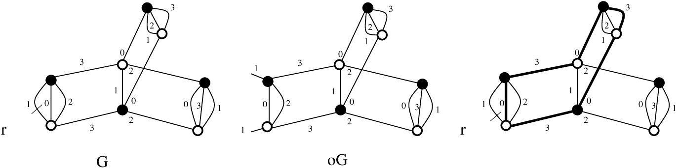
Refer to caption — Figure 1: A colored graph $G$ (where the root edge is represented as crossed), the open colored graph $\mathrm{op}(G)$ , and a face $(0,3)$ of $G$ .

From now on in this article, an integer $D\geq 3$ is fixed.

Definition 1

A rooted, closed, connected colored graph $G$ (henceforth called a colored graph for short) is a connected bipartite $(D+1)$ -regular graph with black and white vertices and colored edges, such that:

•

the colors of edges are taken in the set $\{0,\ldots,D\}$ ,
•

each vertex is incident to exactly one edge of each color,
•

an edge of $G$ , denoted $r(G)$ , is distinguished and it is called the root edge.

Multiple edges are allowed, but, due to the color constraints, self-loops are not. An example is presented in Fig. 1 on the left.

We denote colored graphs by capital letters like $G,G_{1}$ , etc.. We distinguish white vertices by a white dot index ( $v_{\circ},w_{\circ}$ , etc.) and black vertices by a black dot index ( $v_{\bullet},w_{\bullet}$ , etc.).

We include among the colored graphs the trivial colored graphs (or ring graphs) consisting in an edge closing onto itself and having no vertex (see Fig. 2 on the left). The edge is necessarily the root of the graph and has a color $c\in\{0,\ldots,D\}$ , hence there are $D+1$ distinct ring graphs. We denote them $R^{c}$ , where $c$ is the color of the edge.

It will be convenient to regard the edges of a graph as being formed by pairs of matched half-edges (each half-edge being hooked to one of the end vertices of the edge) and to allow for slightly more general structures, called pre-graphs, in which some of the half-edges are left unmatched. From here on half-edges incident to white vertices will be denoted with a white dot index (e.g. $h_{\circ},h^{\prime}_{\circ}$ , etc.) and half-edges incident to black vertex will be denoted with a black dot index (e.g. $h_{\bullet},h^{\prime}_{\bullet}$ , etc.).

Definition 2

A nontrivial open colored graph $\mathbb{G}$ is a pre-graph with exactly two unmatched half-edges $h_{\bullet}$ and $h_{\circ}$ of the same color $c$ , which becomes a colored graph $G$ by matching the two half-edges into an edge of color $c$ and marking this edge as the root edge $r(G)$ of $G$ .

A trivial open colored graph $\mathbb{E}^{c}$ consists in a unique edge of color $c$ with no end vertex and becomes a ring graph $R^{c}$ upon matching the two ends of the edge.

Open colored graphs will be denoted by emphasized capital letters (e.g. $\mathbb{G},\mathbb{G}_{1}$ , etc.).

We denote $\textrm{cl}(\mathbb{G})$ (and call it the closure of $\mathbb{G}$ ) the colored graph obtained by matching the two half-edges of the open colored graph $\mathbb{G}$ into a root edge. Conversely, given a colored graph $G$ , we denote $\textrm{op}(G)$ (and call it the opening of $G$ ) the unique open colored graph $\mathbb{G}$ such that $\textrm{cl}(\mathbb{G})=G$ (see Fig. 1 in the center for an example). Of course, $\textrm{cl}(\mathbb{E}^{c})=R^{c}$ and $\textrm{op}(R^{c})=\mathbb{E}^{c}$ as depicted in Fig. 2 on the right. Open colored graphs are not rooted.

A non trivial open colored graph $\mathbb{G}$ (which is a pre-graph, having two half-edges) can be transformed into a graph $\textrm{Gr}(\mathbb{G})$ by simply erasing the half-edges. Two of the vertices of $\textrm{Gr}(\mathbb{G})$ have coordination $D$ , while all the others have coordination $D+1$ . The edges of $\textrm{Gr}(\mathbb{G})$ are colored.

The following definition is illustrated in figure 3.

Definition 3

An open colored subgraph $\mathbb{H}$ of a nontrivial open colored graph $\mathbb{G}$ , denoted $\mathbb{H}\subset\mathbb{G}$ , is a non trivial open colored graph such that $\mathrm{Gr}(\mathbb{H})$ is a subgraph of $\mathrm{Gr}(\mathbb{G})$ .

By extension an open colored subgraph $\mathbb{H}$ of a colored graph $G$ , denoted $\mathbb{H}\subset G$ is an open colored subgraph of $\mathrm{op}(G)$ .

A half-edge, say $h_{\circ}$ , of an open colored subgraph $\mathbb{H}\subset\mathbb{G}$ can either be one of the half-edges of $\mathbb{G}$ or belong to an edge $e$ of $\mathbb{G}$ , which we denote $h_{\circ}\in e$ .

Let $G$ be a colored graph. In view of the bipartiteness and regularity constraints, $G$ has an equal number $k(G)$ of black and white vertices, and by construction it also has $(D+1)k(G)$ edges. Let us define the faces of $G$ as its bicolored connected components: more precisely, given $0\leq c\neq c^{\prime}\leq D$ , the faces of color $\{c,c^{\prime}\}$ are the connected components of the subgraph consisting of edges that have color $c$ or $c^{\prime}$ , and they form a set of cycles since every vertex in the subgraph has degree 2 (see Fig. 1 on the right for an example). Observe that with this definition the ring graph $R^{c}$ has $D$ faces, one for each color different from $c$ .

Let $F^{cc^{\prime}}_{p}(G)$ denote the number of faces of color $\{c,c^{\prime}\}$ and length $2p$ of the colored graph $G$ . We denote $\smash{F^{cc^{\prime}}(G)=\sum_{p\geq 1}F_{p}^{cc^{\prime}}(G)}$ , $\smash{F_{p}(G)=\sum_{0\leq c<c^{\prime}\leq D}F_{p}^{cc^{\prime}}(G)}$ and $\smash{F(G)=\sum_{p\geq 1}F_{p}(G)}$ , the total number of faces of color $\{c,c^{\prime}\}$ of $G$ , the total number of faces of length $2p$ of $G$ and the total number of faces of $G$ .

Definition 4

Let the reduced degree (the degree for short) of $G$ be the integer $\delta(G)$ defined by the relation:

\delta(G)=\frac{1}{2}D(D-1)k(G)+D-F(G)\;.

(1)

Proposition 1 ([7])

The degree $\delta(G)$ of a non trivial colored graph $G$ is a non negative integer.

Proof

Each of the $D!$ cyclic permutations $\pi$ of the colors $\{0,\ldots,D\}$ induces a unique embedding of the graph $G$ in a compact oriented surface upon requiring that $\pi$ describes the clockwise arrangement of edges around black vertices and the counterclockwise arrangement of edges around white ones. The resulting combinatorial map $G_{\pi}$ , called in [7] a jacket of $G$ , has $(D+1)k(G)$ edges, $2k(G)$ vertices and $\sum_{c}F^{c\,\pi(c)}(G)$ faces since its faces are precisely the faces of color $\{c,\pi(c)\}$ of $G$ . Euler’s formula yields the relation $2k(G)+\sum_{c}F^{c\,\pi(c)}(G)=(D+1)k(G)+2-2g_{\pi}$ , where $g_{\pi}$ denotes the genus of $G_{\pi}$ . Taking into account that each face of $G$ (say with colors $\{c,c^{\prime}\}$ ) is counted by $2(D-1)!$ cycles $\pi$ (those such that $\pi(c)=c^{\prime}$ and those such that $\pi(c^{\prime})=c$ ), we have $\sum_{\pi}\sum_{c}F^{c\,\pi(c)}(G)=2(D-1)!F(G)$ , and upon summing over all $\pi$ we obtain $\delta(G)=\frac{1}{(D-1)!}\sum_{\pi}g_{\pi}$ . The positivity of $\delta(G)$ thus follows from that of the genera of all jackets.

∎

Observe that the degree of a ring graph is zero, $\delta(R^{c})=0$ . The following corollary summarizes the relations we shall need on colored graphs:

Corollary 1

Let $G$ be a nontrivial colored graph with $2k(G)$ vertices, $(D+1)k(G)$ edges, degree $\delta(G)$ and $F(G)$ faces, $F_{p}(G)$ of which have length $2p$ . Then:

$\displaystyle D(D+1)k(G)$	$\displaystyle=$	$\displaystyle 2\sum_{p\geq 1}pF_{p}(G)\;,$	(2)
$\displaystyle D(D-1)k(G)$	$\displaystyle=$	$\displaystyle 2F(G)+2\delta(G)-2D\;,$	(3)
$\displaystyle(D+1)\delta(G)+2F_{1}(G)$	$\displaystyle=$	$\displaystyle D(D+1)+\sum_{p\geq 2}\left[(D-1)p-D-1\right]F_{p}(G)\;.$	(4)

Proof

The first equation follows by observing that in the graph $G$ there are a total of $D(D+1)k(G)$ pairs of edges at vertices of $G$ , and that each such pair is a corner on some face. The second is the definition of the degree. The third one is a simple linear combination of the first two.

∎

Equation (4) already suggests that the classical case $D=2$ , which we do not consider here, is very different from $D\geq 4$ . On the one hand when $D=2$ , the coefficient of $F_{2}(G)$ in the right hand side is negative, so that the number of large faces (or the degree of the largest face) can be arbitrarily large even if $\delta(G)$ and $F_{1}(G)$ are fixed. On the other hand when $D\geq 4$ , the right hand sum has only positive coefficients and the number of large faces (or the degree of the largest face) is bounded by $(D+1)\delta(G)+2F_{1}(G)$ . The case $D=3$ is a priori intermediate in the sense that faces of degree 4 could proliferate at fixed $\delta(G)$ and $F_{1}(G)$ (since the coefficient of $F_{2}(G)$ is zero in this case), but we shall see later that this does not happen, and the dichotomy is really between $D=2$ and $D\geq 3$ .

3 The core of a rooted colored graph

3.1 First attempts to define the core

A melon with external color $c$ (or simply a melon) $\mathbb{O}^{c}$ in a colored graph $G$ is an open colored subgraph of $G$ consisting of $D$ parallel edges joining two vertices, and two half-edges of color $c$ (one on each vertex of $\mathbb{O}^{c}$ ). Depending on the external color $c$ , there are $D+1$ distinct types of melons. The melon removal of $\mathbb{O}^{c}$ in $G$ consists in cutting the two edges of $G$ corresponding to the half-edges of $\mathbb{O}^{c}$ , deleting $\mathbb{O}^{c}$ , and gluing the two remaining half-edges to recreate an edge of color $c$ (see Fig. 4).

We would like to define the core of a rooted colored graph as “the” graph obtained by a maximal sequence of melon removals. However in this “definition”, it is not clear that the core is uniquely defined. We will therefore follow an alternative approach, which is reminiscent of an old result of Tutte [18] about 2-connected graphs, that is, graphs that cannot be disconnected by removing a single vertex. In the modern phrasing of [2], Tutte’s result states that any 2-connected graph $G$ with set of vertices ${\cal{V}}$ and set of edges ${\cal{E}}$ (which we denote $G=({\cal{V}},{\cal{E}})$ ) can be decomposed into an arborescent structure called its RMT-tree by a careful analysis of all its 2-cuts, that is, its pairs $\{x,y\}$ of vertices such that $G|_{{\cal{V}}\setminus\{x,y\}}$ is not connected. Our interest in this result arises from the following lemma.

Lemma 1

Non trivial colored graphs are 2-connected.

Proof

Consider a colored graph $G=({\cal{V}},{\cal{E}})$ containing a white vertex $w_{\circ}$ such that $G^{\prime}=G|_{{\cal{V}}\setminus\{w_{\circ}\}}$ is not connected and let $G_{1}$ be a connected component of $G^{\prime}$ . Let $\ell$ denote the number of edges between $w_{\circ}$ and vertices of $G_{1}$ . By hypothesis there is at least one other connected component in $G^{\prime}$ so that $1\leq\ell\leq D$ . Let us consider the subgraph of $G$ induced by $w_{\circ}$ and the vertices of $G_{1}$ . In this subgraph all the black vertices and all the white vertices except $w_{\circ}$ have degree $D+1$ , while $w_{\circ}$ has degree $1\leq\ell\leq D$ : double counting of edges yields a contradiction.

∎

In view of this lemma one could directly apply Tutte’s result to colored graphs and obtain a decomposition by describing the resulting RMT-trees, and this was our approach in an earlier version of this article. However it turns out to be easier to derive the decomposition we need from a direct analysis of 2-edge-cuts.

2-edge-cuts in colored graphs.

A 2-edge-cut of a 2-connected graph $G=({\cal{V}},{\cal{E}})$ is a pair of edges $\{e,e^{\prime}\}$ such that the graph $G-\{e,e^{\prime}\}=({\cal{V}},{\cal{E}}\setminus\{e,e^{\prime}\})$ is not connected (see Fig. 5 left hand side). Again by double counting of edges, one easily checks that the two edges of a 2-edge-cut in a colored graph must have the same color. A simple cycle of a graph $G$ is a cycle visiting each vertex of $G$ at most once.

Lemma 2

Let $G$ be a 2-connected graph. Then $\{e,e^{\prime}\}$ is a 2-edge-cut in $G$ if and only if any simple cycle visiting $e$ also visits $e^{\prime}$ .

Proof

Let $e=\{x,y\}$ and let $Cycle$ be a simple cycle visiting $e$ . Then $G-\{e,e^{\prime}\}$ has two connected components, one containing $x$ and the other containing $y$ . But $Cycle-e$ is a path from $x$ to $y$ and $e^{\prime}$ is the only edge connecting the two components in $G-\{e\}$ .

Conversely if $\{e,e^{\prime}\}$ is not a 2-edge-cut then there exists a path in $G-\{e,e^{\prime}\}$ between any two vertices, and in particular between the endpoints of $e$ .

∎

Lemma 3

Let $\{e,e^{\prime}\}$ and $\{e,e^{\prime\prime}\}$ be two distinct 2-edge-cuts in a 2-connected graph $G$ . Then $\{e^{\prime},e^{\prime\prime}\}$ is also a 2-edge-cut of $G$ . Moreover if two oriented cycles visit $e$ in the same direction, then they both visit $e^{\prime}$ and $e^{\prime\prime}$ in the same order after $e$ .

Proof

Any cycle visiting $e^{\prime}$ visits also $e$ (since $\{e,e^{\prime}\}$ is a 2-edge-cut) and thus also $e^{\prime\prime}$ (since $\{e,e^{\prime\prime}\}$ is a 2-edge-cut), and we conclude by Lemma 2. Next assume that there exist two oriented cycles $(e,Path_{1},e^{\prime},Path_{1}^{\prime},e^{\prime\prime},Path_{1}^{\prime\prime})$ and $(e,Path_{2},e^{\prime\prime},Path_{2}^{\prime},e^{\prime},Path_{2}^{\prime\prime})$ that visit $e$ in the same direction. But then the path $Path_{2}$ would connect the two connected components of $G-\{e,e^{\prime}\}$ without visiting $e$ or $e^{\prime}$ .

∎

A proper cut-set of a 2-connected graph $G$ is a maximal set $Cut$ of edges such that any 2 edges of $Cut$ form a 2-edge-cut. In view of the previous lemma, an edge can belong to at most one proper cut-set, so that we define the cut-set of an edge as the unique proper cut-set it belongs to if it exists, or the edge itself otherwise.

Lemma 4

Let $G=({\cal{V}},{\cal{E}})$ be a non trivial colored graph and let $e_{0}$ be an edge of $G$ with non-trivial cut-set $Cut$ . Then there exists a unique way to cyclically arrange the edges of $Cut$ as $(e_{0},\ldots,e_{\ell})$ and a unique partition ${\cal{V}}_{0},\ldots,{\cal{V}}_{\ell}$ of ${\cal{V}}$ such that ${\cal{E}}=Cut\cup{\cal{E}}_{{\cal{V}}_{0}}\cup\ldots\cup{\cal{E}}_{{\cal{V}}_{\ell}}$ , where ${\cal{E}}_{{\cal{V}}_{i}}$ are edges connecting only vertices in ${\cal{V}}_{i}$ , and for all $i=0,\ldots,\ell$ , $e_{i}$ connects a black vertex of ${\cal{V}}_{i}$ to a white vertex of ${\cal{V}}_{i+1}$ with indices taken modulo $\ell+1$ (see Fig. 5).

Proof

Since $G$ is 2-connected, there exists a simple cycle visiting $e_{0}$ , and this cycle also visits the other edges in $Cut$ . Orient this cycle so that $e_{0}$ is visited from its black to its white endpoint and let $(e_{0},e_{1},\ldots,e_{\ell})$ describe the cyclic arrangement of the edges of $Cut$ along this oriented cycle. Then $\{e_{i},e_{i+1}\}$ forms a 2-edge-cut and one of the components of $G-\{e_{i},e_{i+1}\}$ contains the edges $e_{i+2},\ldots,e_{i-1}$ . Let ${\cal{V}}_{i}$ denote the vertex set of other component. Then the ${\cal{V}}_{i}$ are disjoint and form a partition of ${\cal{V}}$ and the other required properties are immediate. The uniqueness follows from the fact that any other cycle traversing $e_{0}$ has to visit the edges of $Cut$ in the same order (Lemma 3).

∎

We will be especially interested in the cut-set of the root edge $r(G)$ of a colored graph $G$ . The list $(\mathbb{G}_{0},\ldots,\mathbb{G}_{\ell})$ of open components of the cut-set of the root $r(G)$ is the set of open colored graphs obtained by cutting each edge of this cut-set into two half-edges: with the notation of the lemma, the vertex set of $\mathbb{G}_{i}$ is ${\cal{V}}_{i}$ and the two half-edges of $\mathbb{G}_{i}$ arise from $e_{i}$ and $e_{i+1}$ respectively. The set of closed components of the cut-set of the root is then the set of colored graphs obtained from the open components by reconnecting in each of them the unique available pair of half-edges to form a root edge: $\left(\textrm{cl}(\mathbb{G}_{i}),i=0,\ldots,\ell\right)$ . These definitions are illustrated by Fig. 5.

Finally the following immediate lemma will be useful.

Lemma 5

Let $Cut^{\prime}$ and $Cut^{\prime\prime}$ be two distinct cut-sets in a colored graph $G$ . Then there is an open component $\mathbb{G}^{\prime}$ of $Cut^{\prime}$ containing $Cut^{\prime\prime}$ , and an open component $\mathbb{G}^{\prime\prime}$ of $Cut^{\prime\prime}$ containing $Cut^{\prime}$ .

Proof

Assume $Cut^{\prime\prime}$ is not contained in any of the open components of $Cut^{\prime}$ , and let $e^{\prime\prime}_{i},e^{\prime\prime}_{j}$ be two edges of $Cut^{\prime\prime}$ appearing in two different components $\mathbb{G}^{\prime}_{p}$ and $\mathbb{G}^{\prime}_{q}$ of $Cut^{\prime}$ . Then any cycle visiting $e^{\prime\prime}_{i}$ also visits $e^{\prime\prime}_{j}$ , and thus $e^{\prime}_{p}$ and $e^{\prime}_{p+1}$ and so that $Cut^{\prime}$ and $Cut^{\prime\prime}$ are not disjoint.

∎

3.2 Melons and melonic graphs

An important ingredient in our approach are the open melonic graphs, defined inductively (see Fig. 6) below.

Definition 5

An open colored graph $\mathbb{M}$ with half-edges of color $c$ is a:

•
melonic graph if:
- –
  
  either it is trivial, that is $\mathbb{M}=\mathbb{E}^{c}=\mathrm{op}(R^{c})$ ,
- –
  
  or all the open components of the cut-set of the root edge of $\mathrm{cl}(\mathbb{M})$ are prime melonic graphs.
•

a prime melonic graph if it is non trivial and by cutting all the edges incident to the vertices $v_{\circ}$ and $v_{\bullet}$ of $\mathbb{M}$ which carry the external half-edges of $\mathbb{M}$ into pairs of half-edges and subsequently deleting $v_{\circ}$ , $v_{\bullet}$ and all the half-edges attached to them one obtains $D$ (one for each $c^{\prime}\neq c$ ) open melonic graphs. Observe that if $v_{\circ}$ and $v_{\bullet}$ are connected by an edge in $\mathbb{M}$ , then this edge is cut twice and this creates a trivial melonic graph.

A colored graph $G$ is melonic if $\mathrm{op}(G)$ is an open melonic graph. In particular a ring graph $R^{c}$ is melonic.

In the previous literature (see e.g. [7, 8]) melonic graphs have been defined as the graphs that can be obtained from some ring graph $R^{c}$ by cutting edges and inserting recursively melons $\mathbb{O}^{c^{\prime}}$ . Let us now recall the (known) consistence of this definition with ours. Let $G[e^{c}\leftarrow\mathbb{O}^{c}]$ denote the rooted colored graph obtained by the insertion of a melon $\mathbb{O}^{c}$ at a non-root edge $e^{c}$ (of color $c$ ) of $G$ , i.e. by cutting $e^{c}$ into two half-edges and gluing these half-edges to those of $\mathbb{O}^{c}$ in the unique way that makes the result bipartite. The insertion at the root edge $r(G)=\{v_{\circ},v_{\bullet}\}$ of $G$ can be performed in two ways: either such that the root of $G[r(G)\leftarrow\mathbb{O}^{c}]$ is hooked to the white vertex $v_{\circ}$ or such that the new root edge is hooked to the black vertex $v_{\bullet}$ .

Proposition 2

A colored graph with root edge of color $c$ is melonic if and only if it can be obtained from the ring graph $R^{c}$ by a sequence of melon insertions.

Proof

By induction, observing that the only prime melonic open graphs with two vertices are the $\mathbb{O}^{c}$ s.

∎

Our interest in melonic graphs arises from the following two known results (e.g. [7, 8]):

Proposition 3

The degree of $G$ and $G[e^{c}\leftarrow\mathbb{O}^{c}]$ are the same.

Proof

By construction $G[e^{c}\leftarrow\mathbb{O}^{c}]$ has two more vertices and $\binom{D}{2}$ more faces than $G$ , hence by Equation (3) they have the same degree.

∎

Theorem 3.1

[7, 8] A rooted colored graph $G$ is melonic if and only if it has degree 0.

Proof

Propositions 2 and 3 and the remark that the reduce degree of a ring graph is zero immediately imply that melonic graphs have degree 0.

In order to prove the other implication, observe that if $G$ is non trivial and $\delta(G)=0$ , then from Eq. (4) it ensues that $F_{1}(G)\geq D(D+1)/2$ , hence there exists a face with colors $(c_{1},c_{2})$ of length two (i.e. formed by the two edges $e^{c_{1}}=\{v_{\circ},v_{\bullet}\}$ and $e^{c_{2}}=\{v_{\circ},v_{\bullet}\}$ ) of $G$ .

If for all $c\neq c_{1},c_{2}$ the two vertices are connected by a unique edge $e^{c}=\{v_{\circ},v_{\bullet}\}$ , then $G=R^{c^{\prime}}[e^{c^{\prime}}\leftarrow\mathbb{O}^{c^{\prime}}]$ and $G$ is melonic. Else, there exists $c$ such that the edge of color $c$ hooked to $v_{\circ}$ (denoted $e_{1}^{c}$ ) is different from the edge of color $c$ hooked to $v_{\bullet}$ (denoted $e^{c}_{2}$ ). As $\delta(G)=0$ all the jackets $G_{\pi}$ of $G$ are planar, including $\pi(c_{1})=c,\pi(c)=c_{2}$ , hence $\{e_{1}^{c},e^{c}_{2}\}$ is a 2-edge-cut of $G$ . Cutting $e^{c}_{1}$ and $e^{c}_{2}$ into pairs of half-edges $e^{c}_{1}=\Braket{h^{1}_{\circ},h^{1}_{\bullet}}$ and $e^{c}_{2}=\Braket{h^{2}_{\circ},h^{2}_{\bullet}}$ and reconnecting the half-edges the other way around into two new edges $f_{1}=\Braket{h^{1}_{\circ},h^{2}_{\bullet}}$ and $f_{2}=\Braket{h^{2}_{\circ},h^{1}_{\bullet}}$ , $G$ splits into two colored graphs $G_{1}$ (containing the edge $f_{1}$ ) and $G_{2}$ (containing the edge $f_{2}$ ). Some care must be taken with the root:

•

if $r(G)\neq e^{c}_{1},e^{c}_{2}$ and $r(G)$ belongs let’s say to $G_{1}$ , then $r(G_{1})=r(G)$ and $r(G_{2})=f_{2}$ ,
•

if $r(G)=e^{c}_{1}$ or $r(G)=e^{c}_{2}$ then $r(G_{1})=f_{1}$ and $r(G_{2})=f_{2}$ .

As $k(G_{1})+k(G_{2})=k(G)$ and $F(G_{1})+F(G_{2})=F(G)+D$ , it follows that $\delta(G_{1})=\delta(G_{2})=0$ and taking into account that $k(G_{1}),k(G_{2})<k(G)$ , the theorem follows by induction.

∎

3.3 The core decomposition

Two open colored subgraphs of an open colored graph $\mathbb{G}$ are totally disjoint if their edge sets are disjoint and their half-edges belong to different edges of $\mathbb{G}$ . We shall be particularly interested in open colored subgraphs that are open melonic graphs: for short we refer to these as open melonic subgraphs. Recall that open colored subgraphs are assumed non trivial, and so are open melonic subgraphs.

The following lemma is illustrated in Fig. 7.

Lemma 6

If two open melonic subgraphs of a rooted colored graph $G$ are not totally disjoint then their union is an open melonic subgraph of $G$ .

Proof

First observe that if $\mathbb{M}$ is an open melonic subgraph of $G$ with half-edges $h_{\circ}\in e$ and $h_{\bullet}\in e^{\prime}$ , then the edges $e$ and $e^{\prime}$ of $G$ form a 2-edge-cut of $G$ , unless $e=e^{\prime}=r(G)$ , in which case $\mathbb{M}=\mathrm{op}(G)$ . Indeed, since each vertex of $\mathbb{M}$ has the same degree (counting the half-edges) in $\mathbb{M}$ and in $G$ , all the edges of $G$ incident to a vertex of $\mathbb{M}$ are in $\mathbb{M}$ , except for $e$ and $e^{\prime}$ .

Now if $\mathbb{M}_{1}$ and $\mathbb{M}_{2}$ are two open melonic subgraphs of $G$ with half-edges $h^{1}_{\circ}\in e_{1}$ and $h^{1}_{\bullet}\in e_{1}^{\prime}$ , and $h^{2}_{\circ}\in e_{2}$ and $h^{2}_{\bullet}\in e_{2}^{\prime}$ respectively, then the two cuts $\{e_{1},e_{1}^{\prime}\}$ and $\{e_{2},e_{2}^{\prime}\}$ :

•

either belong to two different cut-sets: in this case, in view of Lemma 5, either $\mathbb{M}_{1}\subset\mathbb{M}_{2}$ or $\mathbb{M}_{2}\subset\mathbb{M}_{1}$ (or $\mathbb{M}_{1}$ and $\mathbb{M}_{2}$ are totally disjoint but this contradict the hypothesis).
•

or belong to the same cut-set: in this case, since $\mathbb{M}_{1}$ and $\mathbb{M}_{2}$ are not totally disjoint, there are two edges $e^{\prime\prime}_{1}\in\{e_{1},e_{1}^{\prime}\}$ and $e^{\prime\prime}_{2}\in\{e_{2},e_{2}^{\prime}\}$ such that $\mathbb{M}_{1}\cup\mathbb{M}_{2}$ is the component of $G-\{e^{\prime\prime}_{1},e^{\prime\prime}_{2}\}$ not containing the root. In particular the closed components of the cut-set of the root of $\textrm{cl}(\mathbb{M}_{1}\cup\mathbb{M}_{2})$ are the union of the closed components of the cut-sets of the roots of $\textrm{cl}(\mathbb{M}_{1})$ and $\textrm{cl}(\mathbb{M}_{2})$ and they are all prime melonic graphs, so that $\mathbb{M}_{1}\cup\mathbb{M}_{2}$ is melonic.

∎

A maximal melonic subgraph of a colored graph $G$ is a (non trivial) open melonic subgraph which is maximal for inclusion.

Lemma 7

The maximal melonic subgraphs of $G$ are totally disjoint.

Proof

This is an immediate consequence of Lemma 6.

∎

Definition 6

The core of an open colored graph $\mathbb{G}$ is the open colored graph $\hat{\mathbb{G}}$ obtained from $\mathbb{G}$ by deleting each of its maximal melonic subgraphs and gluing the resulting pairs of half-edges to reform edges. The core $\hat{G}$ of a colored graph $G$ is the colored graph obtained by deleting each of the maximal melonic subgraphs of $G$ , i.e. $\hat{G}$ is the closure of the core of $\mathrm{op}(G)$ .

Observe that if one of the two half-edges of $\mathbb{G}$ belongs to a melonic subgraph then this half-edge is considered to be cut and re-glued. If both half-edges of $\mathbb{G}$ belong to the same melonic subgraph, then $\mathbb{G}$ is melonic and the core is a trivial one edge graph $\mathbb{E}^{c}$ .

A colored graph is melon-free if it does not contains a melonic subgraph. Observe that according to our conventions, the ring graphs $R^{c}$ are considered melon-free: in view of Proposition 2 they are in fact the only melon-free graphs of degree 0. By construction the core of an open colored graph $\mathbb{G}$ (or of a colored graph $G$ ) is melon-free.

The following characterization (which is in fact not used in the rest of the paper) more generally relates our construction to the initial discussion of this section and is a direct consequence of Proposition 2.

Proposition 4

The core of a colored graph $G$ is the unique melon-free graph that can be obtained from $G$ by a sequence of melon removals (discussed in Section 3.1).

By definition of the core $\hat{G}$ of a colored graph $G$ , for each non-root edge $e=\{w_{\circ},w_{\bullet}\}$ with color $c$ in $\hat{G}$ ,

•

either there is a maximal melonic subgraph in $G$ , which we denote $\mathbb{M}_{e}$ , whose half-edges have color $c$ and respectively point to $w_{\circ}$ and $w_{\bullet}$ ,
•

or there is an edge $\{w_{\circ},w_{\bullet}\}$ with color $c$ in $G$ and this edge is not involved in any melonic subgraph of $G$ , and in this case we set $\mathbb{M}_{e}=\mathbb{E}^{c}$ by convention.

Considering the root edge $r(\hat{G})=\{v_{\circ},v_{\bullet}\}$ of a nontrivial core $\hat{G}$ to be formed of two matched half-edges $h_{\circ}$ and $h_{\bullet}$ , for each of these half-edges:

•

either there is a maximal melonic subgraph denoted $\mathbb{M}_{\circ}$ (resp. $\mathbb{M}_{\bullet}$ ) whose white (resp. black) half-edge is $h_{\circ}$ (resp. $h_{\bullet}$ )
•

or the root edge of $G$ is hooked directly to $v_{\circ}$ (resp. $v_{\bullet}$ ), and in this case we set $\mathbb{M}_{\circ}=\mathbb{E}^{c}$ (resp. $\mathbb{M}_{\bullet}=\mathbb{E}^{c}$ ).

If the core is trivial, that is $\hat{G}=R^{c}$ , then $G$ is melonic: $\mathrm{op}(G)$ is then the (possibly trivial) melonic subgraph $\mathbb{M}_{r(R^{c})}$ associated to the unique edge $r(R^{c})$ of $R^{c}$ .

The core decomposition of a colored graph $G$ is the tuple $(\hat{G};(\mathbb{M}_{\circ},\mathbb{M}_{\bullet},\mathbb{M}_{e_{2}},\ldots,\mathbb{M}_{e_{(D+1)k(\hat{G})}}))$ , where $e_{2},\ldots,e_{(D+1)k(\hat{G})}$ is a canonical list of the edges of $\hat{G}$ excluding the root edge. The following theorem, exemplified in Fig. 8, summarizes and is an immediately consequence of the above discussion.

Theorem 3.2 (Core decomposition)

The core decomposition is one-to-one between

•

colored graphs $G$ with $2k(G)$ vertices and degree $\delta(G)$ ,
•
pairs $(\hat{G};(\mathbb{M}_{\circ},\mathbb{M}_{\bullet},\mathbb{M}_{2}\ldots,\mathbb{M}_{(D+1)k(\hat{G})}))$ where
- –
  
  $\hat{G}$ is a melon-free colored graph with $2k(\hat{G})$ vertices and degree $\delta(\hat{G})=\delta(G)$ , and
- –
  
  for all $i\in\{\circ,\bullet,2,\ldots,(D+1)k(\hat{G})\}$ , $\mathbb{M}_{i}$ is a possibly trivial open melonic graph with $2k(\mathbb{M}_{i})$ vertices,
such that $2k(\hat{G})+\sum_{i}2k(\mathbb{M}_{i})=2k(G)$ .

Proof

The core decomposition is clearly injective since all the components of $G$ have been kept in the decomposition as well as the correspondence between edges of the core and subgraphs. Conversely any such pair yields a rooted colored graph $G$ by substitution of the $\mathbb{M}_{i}$ in $\hat{G}$ and all substituted melonic subgraphs become totally disjoint maximal melonic subgraphs in $G$ , so that $\hat{G}$ is the core of $G$ and the core decomposition gives back the $\mathbb{M}_{i}$ .

The relation between $k(\hat{G})$ , $k(\mathbb{M}_{i})$ and the $k(G)$ follows from the remark that the core decomposition is a partition of the vertex set of $G$ , while the fact that a rooted colored graph and its core have the same degree follows from Proposition 3.

∎

4 Chains

4.1 Maximal chains

The set of cores of fixed degree is not finite. This is due to the presence of chains of $(D-1)$ -dipoles (to be defined precisely below) of arbitrary length. It follows that, in order to provide a useful classification of graphs at fixed degree, we need to refine further the core decomposition by identifying and removing maximal chains. The definition below is slightly different from the one found in [5].

Definition 7

A $(D-q)$ -dipole in a colored graph $G$ is a couple of vertices connected by exactly $D-q$ parallel edges, none of which is the root of the graph. A $(D-q)$ -dipole is attached to the rest of the graph by $q+1$ pairs of half-edges of the same color. It is possible that one of these half-edges belongs to the root edge $r(G)$ or that two of these half-edges are matched to form the root edge $r(G)$ (see Fig. 9 below).

The parallel edges of a dipole are called internal edges of the dipole. The edges of $G$ to which the half-edges of a dipole belong are called external edges of the dipole.

A $(D-1)$ -dipole is said to have external colors $(c_{1},c_{2})$ if a pair of half-edges has color $c_{1}$ and the other one has color $c_{2}$ .

Although dipoles are defined for arbitrary colored graphs, in the rest of the text we will only be interested in dipoles of melon-free colored graphs.

Dipoles can join together to form chains of dipoles (as in Figure 10). The chains of $(D-1)$ -dipoles are especially important: as we will see below, the degree of a graph does not depend of the length of such chains hence all the cores which only differ by the length of the internal chains of $(D-1)$ -dipoles have the same degree.

One would like to identify the maximal vertex disjoint chains of $(D-1)$ -dipoles in a core. The case $D=3$ is slightly subtle and requires a refinement of the naive definition of a chain.

Definition 8

A chain with external colors $(c_{1},c_{2})$ (which can coincide) in a melon-free colored graph $G$ is a connected sub-pre-graph (see Figure 10) made of:

•

two left half-edges $\ell_{\circ}$ and $\ell_{\bullet}$ having the same color $c_{1}$ ,
•

two right half-edges $r_{\bullet}$ and $r_{\circ}$ having the same color $c_{2}$ ,
•

$2p$ internal vertices, $p\geq 1$ , forming a sequence $d_{1},\ldots,d_{p}$ of $(D-1)$ -dipoles,

such that:

•

the white (resp. black) vertex of $d_{1}$ is incident to $\ell_{\circ}$ (resp. $\ell_{\bullet}$ ),
•

the white (resp. black) vertex of $d_{p}$ is incident to $r_{\circ}$ (resp. $r_{\bullet}$ ),
•

two half-edges of the dipole $d_{i}$ are joined to two half-edges of the dipole $d_{i+1}$ for each $i=1,\ldots,p-1$ ,
•

the root of $G$ is not one of the internal edges of the chain (i.e. neither an internal edge of a dipole, nor an edge connecting two consecutive dipoles). Observe however that the root edge can contain one of the half-edges $\ell_{\circ},\ell_{\bullet},r_{\circ},r_{\bullet}$ , or it can consist in any matching of a pair of half-edges: $\Braket{\ell_{\circ},\ell_{\bullet}},\Braket{\ell_{\circ},r_{\bullet}},\Braket{\ell_{\bullet},r_{\circ}}$ or $\Braket{r_{\circ},r_{\bullet}}$ (see Fig. 11).
•

the half-edges $\ell_{\circ},\ell_{\bullet}$ and respectively $r_{\circ},r_{\bullet}$ are not matched together in a non-root edge of $G$ (i.e. the two half-edges at the same end of the chain do not belong to the same non-root edge in $G$ , as in this case the chain would be a melonic subgraph). On the contrary, $\ell_{\circ}$ and $r_{\bullet}$ and respectively $\ell_{\bullet}$ and $r_{\circ}$ can be matched together (see Fig. 11), in a non-root edge.

A chain is proper if it contains at least 4 internal vertices (or equivalently at least two $(D-1)$ -dipoles). A chain is maximal if it is not contained in a larger chain.

With this definition we have the following important results.

Lemma 8

Each chain of $G$ can be extended in a unique way to a maximal chain.

Proof

Let us consider a chain and its two left half-edges $\ell_{\circ}$ and $\ell_{\bullet}$ . If the two half-edges are incident to a $(D-1)$ -dipole in $G$ and neither of the two belongs to the root edge $r(G)$ , then the chain can be extended to the left by adding the $(D-1)$ -dipole. The chain can similarly be extended to the right. The crucial point is that in order to decide whether a chain can be extended, one only tests the half-edges at the same end of the chain.

Extending maximally the chain, one obtains the same maximal chain, irrespective of the order in which the left/right extensions are performed.

∎

A comment is important at this point. Observe that Lemma 8 works because we have allowed a left and right half-edge to be matched in a non-root edge, but it would not work otherwise. Indeed, consider the case at the bottom of Fig. 11. If the chain can be extended only if the left and right half-edges are not matched together, then one obtains two different maximal extensions (including respectively the last dipole on the left or on the right) of the same chain.

Lemma 9

If $D\geq 4$ , two distinct maximal chains in a melon-free colored graph $G$ cannot share an internal vertex. If $D=3$ , two distinct maximal proper chains in a melon-free colored graph $G$ cannot share an internal vertex.

Proof

Assume first that the rooted colored graph $G$ contains two maximal chains that share a $(D-1)$ -dipole. But then these chains are the maximal left/right extension of the dipole, hence coincide.

Now, if two chains share a vertex but no $(D-1)$ -dipoles, then this vertex must belong to two distinct $(D-1)$ -dipoles. Parallel edge count shows that this is not possible for $D\geq 4$ .

As illustrated by the right hand side of Fig. 12, for $D=3$ a vertex $u_{\circ}$ can belong to two 2-dipoles $u_{\circ}-v_{\bullet}$ and $u_{\circ}-w_{\bullet}$ . None of the edges incident at $u_{\circ}$ can be the root edge $r(G)$ . If $u_{\circ}-v_{\bullet}$ belongs to a proper chain, then $w_{\bullet}$ has to belong to the same chain (since the chain has at least 4 internal vertices), hence there exists a vertex $w^{\prime}_{\circ}$ which is connected to $w_{\bullet}$ by a pair of non-root edges and to $u_{\circ}$ by at least one non-root edge.

Applying the same reasoning to the $u_{\circ}-w_{\bullet}$ dipole, we conclude that the graph reduces to a double cycle of length 4 (on the right in Fig. 12), and none of the edges can be the root of $G$ , which is impossible.

∎

Note that, as shown in Fig. 12, in $D=3$ a maximal proper chain can share vertices with a $(D-1)$ -dipole (a 2-dipole), but this is not possible for $D\geq 4$ .

4.2 Classification of chains

There are two main types of proper chains, depending on the way the half-edges are involved in the faces of $G$ .

Let us consider a proper chain with external colors $(c_{1},c_{2})$ , and let us denote the external colors of the first dipole from the left in the chain $(c_{1},c^{\prime})$ . The two left half-edges $\ell_{\circ}$ and $\ell_{\bullet}$ belong to the same face with colors $(c_{1},c)$ for all $c\neq c^{\prime}$ . The last face, with colors $(c_{1},c^{\prime})$ , travels horizontally to the next dipole. Iterating we are in one of the two cases below:

•

either the face $(c_{1},c^{\prime})$ does not travel horizontally through the entire chain, that is there exists a dipole in the chain such that its right external color is neither $c_{1}$ nor $c^{\prime}$ .
•

or the face $(c_{1},c^{\prime})$ travels horizontally along the chain all the way to the right half-edges.

Furthermore the chains can have an even or odd number of dipoles, hence the chains are in one of the two cases below:

•

either the chain has an odd number of dipoles, hence $l_{\circ}$ and $r_{\circ}$ are both on the top of the chain, and $l_{\bullet}$ and $r_{\bullet}$ are both on the bottom.
•

or the chain has an even number of dipoles, hence $l_{\circ}$ and $r_{\bullet}$ are both on the top of the chain, and $l_{\bullet}$ and $r_{\circ}$ are both on the bottom.

Correspondingly the chains are classified into:

Broken chains

A proper chain with external colors $(c_{1},c_{2})$ is broken (or a $B$ chain) if for all $c\neq c_{1}$ , $\ell_{\circ}$ and $\ell_{\bullet}$ are in the same face of color $\{c,c_{1}\}$ and consequently $r_{\circ}$ and $r_{\bullet}$ are in the same face of color $\{c,c_{2}\}$ for all $c\neq c_{2}$ .

Broken chains are subdivided further into chains with equal external colors $c_{2}=c_{1}$ ( $B_{=}$ chains) and chains with distinct external colors, $c_{2}\neq c_{1}$ ( $B_{\neq}$ chains). Furthermore, for each of the two cases the chains can have an even ( $B_{=;\genfrac{}{}{0.0pt}{}{\circ\bullet}{\bullet\circ}}$ resp. $B_{\neq;\genfrac{}{}{0.0pt}{}{\circ\bullet}{\bullet\circ}}$ chains) or an odd ( $B_{=;\genfrac{}{}{0.0pt}{}{\circ\circ}{\bullet\bullet}}$ resp. $B_{\neq;\genfrac{}{}{0.0pt}{}{\circ\circ}{\bullet\bullet}}$ chains) number of dipoles.

Unbroken chains

Chains that are not broken are unbroken ( $U$ chains). Let us consider separately chains of external colors $(c_{1},c_{2}\neq c_{1})$ and $(c_{1},c_{1})$ :

•

external colors $(c_{1},c_{2}\neq c_{1})$ : $\ell_{\circ}$ has color $c_{1}$ and belongs to a face of color $\{c_{1},c_{2}\})$ which does not contain $\ell_{\bullet}$ . This face travels horizontally and leaves the chain through $r_{\circ}$ (which has color $c_{2}$ ). The chain has an odd number of dipoles ( $U_{\neq,\genfrac{}{}{0.0pt}{}{\circ\circ}{\bullet\bullet}}$ chain).
•

external colors $(c_{1},c_{1})$ : again there is a face containing $\ell_{\circ}$ and not $\ell_{\bullet}$ (since the chain is not broken), which has to travel horizontally and leave the chain via $r_{\bullet}$ . There is only one such face traveling horizontally between $\ell_{\circ}$ and $r_{\bullet}$ , with color $\{c_{1},c^{\prime}\}$ (and a parallel face of color $\{c_{1},c^{\prime}\}$ goes through $\ell_{\bullet}$ and $r_{\circ}$ ). The color $c^{\prime}$ is referred to as the secondary color of the unbroken chain. The chain has an even number of dipoles ( $U_{=,\genfrac{}{}{0.0pt}{}{\circ\bullet}{\bullet\circ}}$ chain).

We call internal faces of a chain the faces involving only the internal edges of the chain, and external faces of the chain the faces involving the half-edges.

Lemma 10

The numbers $F^{\rm int}(B)$ of internal faces of a broken proper chain $B$ with $2k(B)$ vertices and $F^{\rm int}(U)$ of internal faces of an unbroken proper chain $U$ with $2k(U)$ vertices are respectively:

F^{\rm int}(B)=\frac{D(D-1)}{2}k(B)-D\;,\qquad F^{\rm int}(U)=\frac{D(D-1)}{2}k(U)-D+1\;.

Proof

By connecting the left (resp. the right) external half-edges of the chain $B$ (resp. $U$ ) into edges $\ell=\Braket{\ell_{\circ},\ell_{\bullet}}$ and $r=\Braket{r_{\circ},r_{\bullet}}$ and marking $\ell$ as root, the chain becomes a melonic graph $G_{B}$ (resp. $G_{U}$ ) with $2k(B)$ (resp. $2k(U)$ ) vertices and $F(G_{B})=F^{\rm int}(B)+2D$ (resp. $F(G_{U})=F^{\rm int}(U)+2D-1$ faces.

∎

We associate to every kind of chain a chain-vertex (see Fig. 13). The chain-vertices have four half-edges, each incident to a black or white square (tracking the vertices of the first respectively last dipole in the chain). For broken chains the top and bottom squares are connected by all the external faces, while for the unbroken ones one external face travels horizontally.

Each chain-vertex admits a minimal realization as a proper chain of $(D-1)$ -dipoles: $B_{=;\genfrac{}{}{0.0pt}{}{\circ\bullet}{\bullet\circ}}$ requires four dipoles, $B_{\neq;\genfrac{}{}{0.0pt}{}{\circ\bullet}{\bullet\circ}}$ requires two dipoles, $B_{=;\genfrac{}{}{0.0pt}{}{\circ\circ}{\bullet\bullet}}$ requires three dipoles, $B_{\neq;\genfrac{}{}{0.0pt}{}{\circ\circ}{\bullet\bullet}}$ requires three dipoles, $U_{\neq,\genfrac{}{}{0.0pt}{}{\circ\circ}{\bullet\bullet}}$ requires three dipoles, $U_{=,\genfrac{}{}{0.0pt}{}{\circ\bullet}{\bullet\circ}}$ requires two dipoles.

5 Schemes

5.1 Reduced schemes and the scheme of a colored graph

Definition 9

A rooted scheme is a connected rooted graph with colored edges having two types of vertices:

•

regular black and white vertices of degree $D+1$ , each incident to one edge of each color,
•

chain-vertices of the 6 types $B_{=;\genfrac{}{}{0.0pt}{}{\circ\bullet}{\bullet\circ}},B_{\neq;\genfrac{}{}{0.0pt}{}{\circ\bullet}{\bullet\circ}},B_{=;\genfrac{}{}{0.0pt}{}{\circ\circ}{\bullet\bullet}},B_{\neq;\genfrac{}{}{0.0pt}{}{\circ\circ}{\bullet\bullet}},U_{\neq,\genfrac{}{}{0.0pt}{}{\circ\circ}{\bullet\bullet}},U_{=,\genfrac{}{}{0.0pt}{}{\circ\bullet}{\bullet\circ}}$ , having two white and two black squares each,

and edges connecting:

•

a black regular vertex and a white regular,
•

a black (or white) regular vertex with a white (or black) square,
•

a black and a white square.

A scheme is reduced if:

•

it is melon free,
•

the left (and right) half-edges of any chain-vertex are not matched together into a non-root edge (they can however be matched in the root edge),
•

the left (or right) half-edges of any chain-vertex or $(D-1)$ -dipole are not matched both at the same time to the left (or right) half-edges of any other chain-vertex or $(D-1)$ -dipole.

Definition 10

The scheme $\tilde{G}$ of a melon-free colored graph $\hat{G}$ is obtained by replacing each maximal proper chain of $\hat{G}$ by the corresponding chain-vertex (since maximal proper chains are vertex disjoint this can be done independently for each chain).

By construction, the scheme of a melon-free colored graph is reduced.

Observe that for $D=3$ , replacing simultaneously the maximal chains of a melon-free colored graph by chain-vertices is not always possible: isolated $(D-1)$ -dipoles are chains (although not proper chains), and are not necessarily vertex disjoint. This is why we restrict our attention to maximal proper chains.

The following theorem is an immediate consequence of the previous discussion.

Theorem 5.1

There is a bijection between the set of melon-free colored graphs $\hat{G}$ with $2k(\hat{G})$ vertices and the set of pairs $(\tilde{G};(C_{1},\ldots,C_{q}))$ where $\tilde{G}$ is a reduced scheme with $q$ chain-vertices $x_{1},\ldots,x_{q}$ , and $C_{i}$ is a chain of the same type as $x_{i}$ , such that the total number of vertices in $\tilde{G}$ and the chains $C_{1},\ldots,C_{q}$ is $2k(\hat{G})$ .

The chain-vertices we have introduced allow to keep track in $\tilde{G}$ of the faces of the melon-free graph that are not internal faces of some chain. The following result is a direct consequence of Lemma 10 and the definition of the degree, Eq. (1).

Lemma 11

Let $\hat{G}_{1}$ and $\hat{G}_{2}$ be two melon-free rooted colored graphs with the same scheme $\tilde{G}$ . Then $\hat{G}_{1}$ and $\hat{G}_{2}$ have the same degree.

Definition 11

The degree of a reduced scheme is the common degree of all cores that have it as scheme.

5.2 Schemes of fixed degree

Our main interest in schemes is that unlike the set of cores of fixed degrees, the set of reduced schemes of fixed degree is finite.

Theorem 5.2

The number of reduced schemes with a fixed degree is finite.

Proof

The proof of this is divided into two parts. First we analyze the iterative elimination of chain-vertices, $(D-1)$ -dipoles, and in the cases $D\geq 4$ , $(D-2)$ -dipoles in a reduced scheme, to prove the following result:

Proposition 5

The number of chain-vertices, $(D-1)$ , and for $D\geq 4$ , $(D-2)$ -dipoles in a reduced scheme of degree $\delta$ is bounded by $19\delta$ .

Proof

See Section 6.

∎

Once this result is granted, we observe that the minimal realization of any chain-vertex consists of at most four $(D-1)$ -dipoles, so that there is an injective map from the reduced schemes of degree $\delta$ into melon free colored graphs of degree $\delta$ with at most $76\delta$ $(D-1)$ - and $(D-2)$ -dipoles.

We then establish the following result:

Proposition 6

For $D=3$ , the number of melon free colored graphs with fixed degree and a fixed number of 2-dipoles is finite. For $D\geq 4$ , the number of melon free colored graphs with fixed degree and fixed numbers of $(D-1)$ -dipoles and $(D-2)$ -dipoles is finite.

Proof

See Section 7.

∎

Theorem 5.2 is an immediate consequence of these two propositions.

∎

6 Proof of Proposition 5

As a preliminary we analyze the effect that the deletion of a single $(D-q)$ -dipole has on the degree. We then extend the analysis to the deletion of a chain-vertex. The conclusion of this analysis is that the deletion of a $(D-q)$ -dipole:

•

either separates the graph into $q+1$ connected components (completely separating deletion), in which case the degree is distributed among the connected components,
•

or it separates the graph into less than $q+1$ connected components, in which case the degree strictly decreases.

Similarly, for chains, the deletion:

•

either separates the graph into two connected components, in which case the degree is distributed among the connected components,
•

or it does not separate the graph, in which case the degree strictly decreases.

6.1 Analysis of a $(D-q)$ -dipole removal

Let us define more precisely the removal of a $(D-q)$ -dipole (with $1\leq q\leq D-2$ ) in a colored graph $G$ : assuming the half-edges of the dipole have colors $c_{0},c_{1},\dots c_{q}$ , we delete the two vertices, the internal edges and the half-edges of the dipole and form one new edge for each color $c_{0},c_{1},\dots c_{q}$ with the remaining pairs of half-edges in $G$ .

By construction, the number of vertices decreases by 2 and the number of edges decreases by $D+1$ at a deletion. In order to track the variation of the degree we need to analyze more precisely the variation of the number of faces. This is somewhat involved, as it depends on the number of connected components the graph separates into upon removal of the $(D-q)$ -dipole and also on whether couples of new edges belong to a same face or not.

Connected components and faces after a dipole removal.

We denote:

G_{1},G_{2},\dots G_{C}\;,

the $C$ connected components obtained after the removal of the $(D-q)$ -dipole, $1\leq C\leq q+1$ . As the removal of the dipole deletes two vertices we have

k(G)=k(G_{1})+k(G_{2})+\dots+k(G_{C})+1\;.

We denote $t_{1}$ the number of new edges belonging to $G_{1}$ , $t_{2}$ the number of new edges belonging to $G_{2}$ , and so on. We have:

t_{1}+t_{2}+\dots+t_{C}=q+1\;.

Without loss of generality we can assume that the colors of the $t_{1}$ new edges belonging to $G_{1}$ are $c_{0},\dots c_{t_{1}-1}$ , the colors of the $t_{2}$ new edges belonging to $G_{2}$ are $c_{t_{1}},\dots c_{t_{1}+t_{2}-1}$ and so on.

The faces affected by the $(D-q)$ -dipole removal are the ones containing at least one of its vertices. They fall into three categories:

•

Faces with colors $\{c,c^{\prime}\}$ such that $\{c,c^{\prime}\}\cap\{c_{0},c_{1},\dots c_{q}\}=\emptyset$ . For each of the $\binom{D-q}{2}$ choices of such pairs, exactly one face of degree two (an internal face of the dipole) is deleted by the removal of the dipole:

$F^{cc^{\prime}}(G)=F^{cc^{\prime}}(G_{1})+F^{cc^{\prime}}(G_{2})+\dots+F^{cc^{\prime}}(G_{C})+1\;,$
•

Faces with colors $\{c_{i},c\}$ , with $c_{i}\in\{c_{0},c_{1},\dots c_{q}\}$ and $c\notin\{c_{0},c_{1},\dots c_{q}\}$ . For each of the $(D-q)(q+1)$ choices of such pairs, exactly one face is incident to the dipole: this face has length at least four in $G$ and the dipole removal reduces its length by 2, so that the number of faces with these colors is unchanged:

$F^{c_{i}c}(G)=F^{c_{i}c}(G_{1})+F^{c_{i}c}(G_{2})+\dots+F^{c_{i}c}(G_{C})\;,$
•
Faces with colors $\{c_{i},c_{j}\}$ with $\{c_{i},c_{j}\}\subset\{c_{0},c_{1},\dots c_{q}\}$ . For each of the $\binom{q+1}{2}$ choices of such colors, either one or two faces are incident to the dipole. In this case we distinguish between two possibilities:
- –
  
  Type $a$ . (Fig. 15) The four edges of color $c_{i}$ and $c_{j}$ belong to the same face of color $\{c_{i},c_{j}\}$ in $G$ . Upon removal of the $(D-q)$ -dipole this face of color $\{c_{i},c_{j}\}$ splits into two disjoint faces:
  
  $F^{c_{i}c_{j}}(G)=F^{c_{i}c_{j}}(G_{1})+F^{c_{i}c_{j}}(G_{2})+\dots+F^{c_{i}c_{j}}(G_{C})-1\;.$
  
  Figure 15: A face which splits by deleting a dipole.
- –
  
  Type $b$ . (Fig. 16) The four edges of color $c_{i}$ and $c_{j}$ belong to two distinct faces $\{c_{i},c_{j}\}$ in $G$ . Upon removal of the $(D-q)$ -dipole the two faces $\{c_{i},c_{j}\}$ are merged into a unique face:
  
  $F^{c_{i}c_{j}}(G)=F^{c_{i}c_{j}}(G_{1})+F^{c_{i}c_{j}}(G_{2})+\dots+F^{c_{i}c_{j}}(G_{C})+1\;.$
  
  Figure 16: Two faces which merge by deleting a dipole.

A third possibility, namely that the two pairs of edges of color $\{c_{i},c_{j}\}$ belong to the same face before the removal and the face does not split, does not exist because the graph $G$ is bipartite.

We are now in position to describe the global effect of the removal of a dipole on the degree.

Case I. Completely separating $(D-q)$ -dipoles.

We first consider the case in which the removal of $(D-q)$ -dipoles splits the graph into $q+1$ connected components each containing exactly one new edge ( $C=q+1$ with the notation above): we refer to such a dipole as completely separating. We illustrated this case in Fig. 17.

In this case all the faces of colors $\{c_{i},c_{j}\}$ with $\{c_{i},c_{j}\}\subset\{c_{0},c_{1},\dots c_{q}\}$ are of Type $a$ , hence

	$\displaystyle F(G)$	$\displaystyle=F(G_{1})+F(G_{2})+\dots+F(G_{q+1})+\binom{D-q}{2}-\binom{q+1}{2}$
		$\displaystyle=F(G_{1})+F(G_{2})+\dots+F(G_{q+1})+\frac{1}{2}{D(D-2q-1)}\;.$

From Eq. (1) we get:

		$\displaystyle\delta(G)=\frac{1}{2}D(D-1)k(G)+D-F(G)$
		$\displaystyle\qquad=\frac{1}{2}D(D-1)\Bigl(k(G_{1})+k(G_{2})+\dots+k(G_{q+1})+1\Bigr)+D$
		$\displaystyle\qquad\quad-\Big(F(G_{1})+F(G_{2})+\dots+F(G_{q+1})+\frac{1}{2}{D(D-2q-1)}\Big)$
		$\displaystyle\qquad=\delta(G_{1})+\delta(G_{2})+\dots+\delta(G_{q+1})\;.$

In conclusion the degree is distributed between the connected components created by the removal of a completely separating dipole.

Case II. Non completely separating $(D-q)$ -dipoles.

We now consider the remaining cases ( $1\leq C\leq q$ ): we refer to such a dipole as non completely separating.

All the faces $\{c_{i},c_{j}\}$ with $c_{i}\in\{c_{0},\dots c_{t_{1}-1}\}$ and $c_{j}\notin\{c_{0},\dots c_{t_{1}-1}\}$ are of Type $a$ . On the contrary the faces $\{c_{i},c_{j}\}$ with $\{c_{i},c_{j}\}\subset\{c_{0},\dots c_{t_{1}-1}\}$ can be either of Type $a$ or of Type $b$ .

Let us denote $b_{1}$ the number of faces of Type $b$ , $0\leq b_{1}\leq\binom{t_{1}}{2}$ in $G_{1}$ , $b_{2}$ the number of faces of Type $b$ in $G_{2}$ and so on. We have:

	$\displaystyle F(G)=$	$\displaystyle F(G_{1})+F(G_{2})+\dots+F(G_{C})+\binom{D-q}{2}-\binom{q+1}{2}$
		$\displaystyle\qquad+2b_{1}+2b_{2}+\dots+2b_{C}$
	$\displaystyle=$	$\displaystyle F(G_{1})+F(G_{2})+\dots+F(G_{C})+\frac{1}{2}D(D-2q-1)$
		$\displaystyle\qquad+2b_{1}+2b_{2}+\dots+2b_{C}\;.$

Using again Eq. (1) we get:

	$\displaystyle\delta(G)=$	$\displaystyle\frac{1}{2}D(D-1)k(G)+D-F(G)$
	$\displaystyle=$	$\displaystyle\frac{1}{2}D(D-1)\Bigl(k(G_{1})+k(G_{2})+\dots+k(G_{C})+1\Bigr)+D$
		$\displaystyle-\Big(F(G_{1})+F(G_{2})+\dots+F(G_{C})$
		$\displaystyle\qquad\qquad+\frac{1}{2}{D(D-2q-1)}{}+2b_{1}+2b_{2}+\dots+2b_{C}\Big)$
	$\displaystyle=$	$\displaystyle\delta(G_{1})+\delta(G_{2})+\dots+\delta(G_{C})$
		$\displaystyle+D(q+1-C)-2b_{1}-2b_{2}-\dots-2b_{C}\;.$

In other terms the variation of the degree through the removal depends on the structure of the incident faces. Observe that, as $b_{i}\leq\binom{t_{i}}{2}$ :

		$\displaystyle D(q+1-C)-2b_{1}-2b_{2}-\dots-2b_{C}\geq D(q+1-C)-t_{1}(t_{1}-1)-\dots t_{C}(t_{C}-1)$		(5)
		$\displaystyle=(D-t_{1})(t_{1}-1)+\dots(D-t_{C})(t_{C}-1)\;,$		(6)

as $t_{1}+\dots+t_{C}=q+1$ . For non completely separating deletions we have $t_{i}\geq 1$ and at least one of them (say $t_{1}$ ) is in fact at least $2$ , hence

(D-t_{1})(t_{1}-1)+\dots(D-t_{C})(t_{C}-1)\geq D-t_{1}\geq D-(q+1)\geq 1

We now make the various possibilities more explicit in the cases of $(D-1)$ - and $(D-2)$ -dipoles:

Non separating $(D-1)$ -dipoles.

We have $q=1$ , $C=1$ and $t_{1}=2$ . Depending on the value of $b_{1}$ we thus distinguish two cases:

•

Case II.A: the face $(c_{0},c_{1})$ is of Type $a$ , hence $b_{1}=0$ and:

$\delta(G)=\delta(G_{1})+D\;.$
•

Case II.B: the face $(c_{0},c_{1})$ is of Type $b$ , $b_{1}=1$ and:

$\delta(G)=\delta(G_{1})+D-2\;.$

Non completely separating $(D-2)$ -dipoles.

We have $q=2$ and there are two possible values for $C$ , and a total of $6$ possible cases:

•
non separating $(D-2)$ -dipole deletion: $C=1$ , $t_{1}=3$ , hence:
- –
  
  $b_{1}=0$ , $\delta(G)=\delta(G_{1})+2D$ .
- –
  
  $b_{1}=1$ , $\delta(G)=\delta(G_{1})+2D-2$ .
- –
  
  $b_{1}=2$ , $\delta(G)=\delta(G_{1})+2D-4$ .
- –
  
  $b_{1}=3$ , $\delta(G)=\delta(G_{1})+2D-6$ .
•
partially separating $(D-2)$ -dipole deletion: $C=2$ , $t_{1}=1$ (hence $b_{1}=0$ ), $t_{2}=2$ , hence:
- –
  
  $b_{2}=0$ , $\delta(G)=\delta(G_{1})+\delta(G_{2})+D$ .
- –
  
  $b_{2}=1$ , $\delta(G)=\delta(G_{1})+\delta(G_{2})+D-2$ .

In conclusion, the degree decreases by at least $D-2$ by removal of a non separating $(D-1)$ -dipole, and for $D\geq 4$ the degree decreases by at least $D-2$ by removal of a non separating or partially separating $(D-2)$ -dipole.

6.2 Chain-vertex removal

The removal of a chain-vertex consists in deleting this vertex and the incident half-edges and creating two new edges by joining the half-edges that arise from the same extremity of the chain-vertex. The removal of a chain-vertex in a scheme $\tilde{G}$ can equivalently be performed in the following way:

•

replace the chain-vertex by its minimal length chain representation: this yields a scheme $\tilde{G}^{\prime}$ with same degree.
•

remove one of the $(D-1)$ -dipole of the inserted chain: one of the three cases above applies.
•

eliminate the melons that might have been created: these operations do not affect the degree.

This last procedure, although slightly more complex a priori, allows to built on the case analysis already done for $(D-1)$ -dipole removal.

Case I. Separating chain-vertex.

The removal of a chain-vertex separates $\tilde{G}$ into two components $\tilde{G}_{1}$ and $\tilde{G}_{2}$ if and only if the deletion of any $(D-1)$ -dipole of the equivalent chain separates the graph $\tilde{G}^{\prime}$ into two components $\tilde{G}^{\prime}_{1}$ and $\tilde{G}^{\prime}_{2}$ . In such a case,

\delta(\tilde{G})=\delta(\tilde{G}^{\prime})=\delta(\tilde{G}^{\prime}_{1})+\delta(\tilde{G}^{\prime}_{2})=\delta(\tilde{G}_{1})+\delta(\tilde{G}_{2}).

Observe that in this case, the chain-vertex can represent indifferently an unbroken or a broken chain.

Case II. Non-separating chain-vertex, broken chain.

Let us call $(c_{1},c^{\prime})$ the external colors of the first dipole in the chain. This case is similar to a Case II.A removal of a $(D-1)$ -dipole: the removal of the chain-vertex does not separate $\tilde{G}$ and in the resulting scheme $\tilde{G}_{1}$ the two new edges belong to two different $(c_{1},c^{\prime})$ -cycles. Then the removal of the chain-vertex is equivalent to a Case II.A removal of $(D-1)$ -dipole in the graph $\tilde{G}^{\prime}$ , followed by some melon deletions:

\delta(\tilde{G})=\delta(\tilde{G}^{\prime})=\delta(\tilde{G}_{1})+D\;.

Case III. Non-separating chain-vertex, unbroken chain.

Let us call $(c_{1},c_{2})$ the external colors of the chain-vertex if they are different, or we call the secondary color of the chain vertex $c_{2}$ , if the external colors are $(c_{1},c_{1})$ . We have two sub cases:

•

Case III.a: two resulting faces. This case is similar to a Case II.A removal of a $(D-1)$ -dipole: the removal of the chain-vertex does not separate $\tilde{G}$ and in the resulting scheme $\tilde{G}_{1}$ the two new edges belong to two different $(c_{1},c_{2})$ -cycles. Then the removal of the chain-vertex is equivalent to a Case II.A removal of $(D-1)$ -dipole in the graph $\tilde{G}^{\prime}$ , followed by some melon deletions:

$\delta(\tilde{G})=\delta(\tilde{G}^{\prime})=\delta(\tilde{G}_{1})+D\;.$
•

Case III.b: single resulting face. This case is similar to a Case II.B removal of a $(D-1)$ -dipole: the removal of the chain-vertex does not separate $\tilde{G}$ but in the resulting scheme $\tilde{G}_{1}$ the two new edges belong to a same $(c_{1},c_{2})$ -cycle. The removal of the chain-vertex is equivalent to a Case II.B removal of $(D-1)$ -dipole in the graph $\tilde{G}^{\prime}$ , followed by some melon deletions:

$\delta(\tilde{G})=\delta(\tilde{G}^{\prime})=\delta(\tilde{G}_{1})+D-2\;.$

6.3 Iterative deletion of chain-vertices, $(D-1)$ -dipoles and $(D-2)$ -dipoles

We now present an algorithm which allows us to eliminate one by one chain vertices and $(D-1)$ -dipoles (and, for $D\geq 4$ , $(D-2)$ -dipoles) in a reduced scheme. This will allow us to show that the total number of chain vertices, $(D-1)$ -dipoles and $(D-2)$ -dipoles in a reduced scheme is bounded linearly in terms of the degree. This algorithm is not unique: we present here an adaptation of a similar one introduced in [12]. For $D=3$ , the algorithm goes through ignoring the $(D-2)$ -dipoles.

The deletions of chain vertices and $(D-1)$ -dipoles can either be completely separating or not separating. The deletions of $(D-2)$ -dipoles can be completely separating, partially separating or non separating. Under any completely separating deletion the degree is distributed among the resulting connected components, while under the non completely separating deletions the degree decreases by at least $D-2$ .

Non completely separating deletions

We will first perform a maximal number of non completely separating deletions, that is non separating deletions of chain vertices and $(D-1)$ -dipoles and non separating or only partially separating deletions of $(D-2)$ -dipoles. Some examples of the algorithm we present below are depicted in Fig. 18 and Fig. 19.

Let $\tilde{G}$ be a reduced scheme of degree $\delta(\tilde{G})$ , and let us denote $\mathfrak{D}(\tilde{G})$ the total number of chain vertices, $(D-1)$ -dipoles and $(D-2)$ -dipoles in $\tilde{G}$ . As long we find a non separating chain-vertex, a non separating $(D-1)$ -dipole formed by parallel unmarked edges or a non completely separating $(D-2)$ -dipole formed by parallel unmarked edges we delete it. We mark the new edges with a blue mark, keeping track of the multiplicity. That is, if the two half-edges connected at a step come from edges having $m_{1;{\rm blue}}$ and $m_{2;{\rm blue}}$ blue marks respectively, the new edge will have $m_{1;{\rm blue}}+m_{2;{\rm blue}}+1$ blue marks. Observe that the deletion of a chain-vertex having a left and a right half-edge matched into an edge creates only one edge with two blue marks. As we delete partially separating $(D-2)$ -dipoles the scheme can become disconnected and one can obtain ring components with blue marks, see Fig. 18 and Fig. 19.

Our aim is to delete at each step only dipoles which were present in the original scheme, hence we only delete dipoles with unmarked parallel edges. If the deletion creates new $(D-1)$ -dipoles and $(D-2)$ -dipoles having blue marks on some of their parallel edges, these edges do not count when identifying dipoles. However, the ring components consisting in one edge with blue marks count as connected components when deciding whether a deletion is completely separating or not.

Observe that $\mathfrak{D}(\tilde{G})$ always goes down by one under a chain-vertex deletion, but, for $3\leq D\leq 5$ it can go down by as much as $3$ for the dipole deletions (see Fig. 18):

•

in $D=3$ the $2$ -dipoles (i.e. $(D-1)$ -dipoles) are not necessarily vertex disjoint. Each vertex of a $2$ -dipole can belong to another $2$ -dipole, in which case three dipoles are erased by a deletion.
•

in $D=4$ the $3$ -dipoles and $2$ -dipoles (i.e. $(D-1)$ -dipoles and $(D-2)$ -dipoles) and couples of $2$ -dipoles (i.e. $(D-2)$ -dipoles) are not necessarily vertex disjoint and again up to three dipoles can be erased at one step.
•

in $D=5$ the $3$ -dipoles (i.e. $(D-2)$ -dipoles) are not necessarily vertex disjoint and again up to three dipoles can be erased at one step.

Observe that if two dipoles share a vertex, then neither of the two can be completely separating.

We iterate the non completely separating deletions maximally and obtain a scheme $\tilde{G}^{\prime}$ . Unlike $\tilde{G}$ , $\tilde{G}^{\prime}$ in general is neither connected nor reduced (as depicted for instance in Fig. 18 and Fig. 19). Furthermore, $\tilde{G}^{\prime}$ is not unique, and depends of the sequence of deletions performed.

The degree of $\tilde{G}^{\prime}$ is the sum of the degrees of its connected components. Let us denote the maximal number of non completely separating deletions one can perform starting from a reduced scheme by $q_{\rm{n.c.s.}}$ . We have the following inequalities:

•

the degree goes down by at least one for each of these deletions, hence:

$q_{\rm{n.c.s.}}\leq\delta(\tilde{G}^{\prime})+q_{\rm{n.c.s.}}\leq\delta(\tilde{G})\;,$

•

$\mathfrak{D}(\tilde{G})$ goes down by at most three at each step, hence:

\mathfrak{D}(\tilde{G})\leq\mathfrak{D}(\tilde{G}^{\prime})+3q_{\rm{n.c.s.}}\leq\mathfrak{D}(\tilde{G}^{\prime})+3\delta(\tilde{G})\;,

•

every deletion creates at most three new blue marks, hence the total number of marks $\tilde{G}^{\prime}$ , $m_{\rm{blue}}(\tilde{G}^{\prime})$ , is bounded by:

$m_{\rm blue}(\tilde{G}^{\prime})\leq 3q_{\rm{n.c.s.}}\leq 3\delta(\tilde{G})\;.$

In the scheme $\tilde{G}^{\prime}$ , all the chain-vertices, $(D-1)$ and $(D-2)$ -dipoles are completely separating. It follows that, for any $D$ , all the remaining $(D-1)$ and $(D-2)$ -dipoles are vertex disjoint.

In order to conclude that $\mathfrak{D}(\tilde{G})$ is bounded linearly in terms of $\delta(\tilde{G})$ , it is enough to bound $\mathfrak{D}(\tilde{G}^{\prime})$ in terms of $\delta(\tilde{G}^{\prime})$ and $m_{\rm{blue}}(\tilde{G}^{\prime})$ . This is slightly subtle because the remaining deletions are all separating, hence they conserve the degree.

All the remaining $(D-1)$ - and $(D-2)$ -dipoles are vertex disjoint, hence we can delete them together with the remaining chain-vertices in any order. We mark the new edges with a black mark, keeping track of the multiplicity (and of course of the multiplicity of the blue marks). That is, if the two half-edges connected at a step come from edges having $m_{1;{\rm black}}$ and $m_{1;{\rm blue}}$ respectively $m_{2;{\rm black}}$ and $m_{2;{\rm blue}}$ black and blue marks, the new edge will have $m_{1;{\rm black}}+m_{2;{\rm black}}+1$ black marks and $m_{1;{\rm blue}}+m_{2;{\rm blue}}$ blue marks.

For each $(D-2)$ -dipole deleted (having external colors, say, $c_{1},c_{2}$ and $c_{3}$ ) we add a copy of the fundamental melon (consisting in two vertices connected by $D+1$ edges) and add a black mark on its edges $c_{1},c_{2}$ and $c_{3}$ . Of course, edges with either type of marks (black or blue) do not count when identifying $(D-2)$ and $(D-1)$ -dipoles.

As before, these deletions can create ring components with marks. We represent in Fig. 20 the deletion of a maximal set of non separating dipoles and chain vertices, followed by the deletion of all the separating $(D-1)$ and $(D-2)$ -dipoles and chain vertices in a reduced scheme.

Let us denote the scheme obtained in this way by $\tilde{G}^{\prime\prime}$ . By construction $\tilde{G}^{\prime\prime}$ has:

•

blue and black marks. The number of blue marks of $\tilde{G}^{\prime\prime}$ is equal to the number of blue marks of $\tilde{G}^{\prime}$ , $m_{\rm blue}(\tilde{G}^{\prime\prime})=m_{\rm blue}(\tilde{G}^{\prime})$ . We denote $m_{\rm black}(\tilde{G}^{\prime\prime})$ the number of black marks in $\tilde{G}^{\prime\prime}$ .
•

the same degree as $\tilde{G}^{\prime}$ .
•

ring components with marks (either blue or black).
•

no $(D-1)$ -dipole made of unmarked parallel edges.
•

no chain-vertex.
•

all the $(D-2)$ -dipoles made of unmarked parallel edges are copies of the fundamental melon with three marked edges.
•

at least a mark (blue or black) in every connected component (or no mark and only one connected component if no dipole or chain-vertex is ever deleted).

The connected components of $\tilde{G}^{\prime\prime}$ can be seen as the vertices of an abstract graph $\mathfrak{F}$ (represented in Fig. 20 at the bottom) whose edges correspond either to the chain-vertices and to the $(D-1)$ -dipoles in $\tilde{G}^{\prime}$ , or to pairs of half-edges of the same color of the $(D-2)$ -dipoles in $\tilde{G}^{\prime}$ . A subtle point is the following (see Fig. 20): a pair of half-edges of the same color of a $(D-2)$ -dipole in $\tilde{G}^{\prime}$ can lead:

•

either to an edge and a vertex in $\mathfrak{F}$ if the pair is matched to a pair of half-edges of a chain-vertex, $(D-1)$ - or $(D-2)$ -dipole, (this is the case of the left and right pairs around the middle dipole in Fig. 20)
•

or to just an edge in $\mathfrak{F}$ if it is not (this is the case of the bottom pair around the middle dipole in Fig. 20).

As all the chain vertices and $(D-1)$ - and $(D-2)$ -dipoles of $\tilde{G}^{\prime}$ are completely separating, $\mathfrak{F}$ is a forest : every tree in $\mathfrak{F}$ corresponds to one of the connected components of $\tilde{G}^{\prime}$ . We denote $\mathfrak{D}^{(D-1)}$ the number of chain vertices and $(D-1)$ -dipoles of $\tilde{G}^{\prime}$ and $\mathfrak{D}^{(D-2)}$ the number of $(D-2)$ -dipoles of $\tilde{G}^{\prime}$ , hence:

\mathfrak{D}(\tilde{G}^{\prime})=\mathfrak{D}^{(D-1)}+\mathfrak{D}^{(D-2)}\;,\qquad\mathfrak{D}^{(D-1)}+3\mathfrak{D}^{(D-2)}=E(\mathfrak{F})\;,

where $E(\mathfrak{F})$ denotes the number of edges of the abstract forest $\mathfrak{F}$ ,

The following lemma characterizes the components of degree zero having only black marks in $\tilde{G}^{\prime\prime}$ .

Lemma 12

The components of degree zero having only black marks of $\tilde{G}^{\prime\prime}$ and not containing the root:

•

either are rings with only two marks such that at least one of the marks comes from a $(D-2)$ -dipole deletion,
•

or have at least three marks.

Proof

The crucial observation is that all the unmarked edges in $\tilde{G}^{\prime\prime}$ are in fact edges which were present in $\tilde{G}$ , and $\tilde{G}$ is a reduced scheme.

The components of degree zero of $\tilde{G}^{\prime\prime}$ are either ring components or melonic graphs with at least two vertices.

Ring components with one black mark can be created by separating deletions only if one deletes $D-1$ edges in a melon $\mathbb{O}^{c}$ in $\tilde{G}$ , one deletes a chain-vertex whose left (or right) external half-edges are matched together into an edge in $\tilde{G}$ or one deletes $D-2$ edges in a $(D-1)$ -dipole of $G$ . The first two cases are impossible as $\tilde{G}$ is reduced, while the third would mean that a dipole of $\tilde{G}$ has been mislabeled.

Ring components with two marks can be created by the deletion of only $(D-1)$ -dipoles and chain vertices only if, in $\tilde{G}$ , the two left (or right) half-edges of a $(D-1)$ -dipole or a chain-vertex are both matched to the two left (or right) half-edges of another $(D-1)$ -dipole or a chain-vertex. This is again impossible, as $\tilde{G}$ is reduced.

Ring components with three marks can be created, as depicted in Fig. 21 below.

A nontrivial melonic graph with fewer than three marks contains at least a $(D-1)$ -dipole made of unmarked parallel edges, which is impossible by the construction of $\tilde{G}^{\prime\prime}$ .

∎

The remainder of the proof relies on the observation that $\mathfrak{F}$ is a finite forest as it has a finite number of vertices of valence zero or one (as only the root component, the strictly positive degree components, and the zero degree components with blue marks of $\tilde{G}^{\prime\prime}$ can be zero valent or univalent in $\mathfrak{F}$ ) and a finite number of vertices of valence two (as this number is bounded linearly in the number of $(D-2)$ -dipoles in $\tilde{G}^{\prime}$ ). We denote:

•

$n_{+}\leq\delta(\tilde{G}^{\prime})$ the number of connected components of $\tilde{G}^{\prime\prime}$ having strictly positive degree.
•

$n_{0,{\rm blue}}\leq m_{\rm blue}(\tilde{G}^{\prime})$ the number of connected components of $\tilde{G}^{\prime\prime}$ having degree zero and having at least a blue mark.
•

$n_{0,{\rm black}}^{(2)}\leq 3\mathfrak{D}^{(D-2)}$ the number of connected components of degree zero of $\tilde{G}^{\prime\prime}$ having exactly two black marks and no blue mark. They are necessarily ring components and at leas one of the marks comes from a $(D-2)$ -dipole deletion.
•

$n_{0,{\rm black}}^{(3)}$ the number of connected components of degree zero of $\tilde{G}^{\prime\prime}$ having only black marks and having at least three marks.

We have:

	$\displaystyle 1+n_{+}+n_{0,{\rm blue}}+n_{0,{\rm black}}^{(2)}+n_{0,{\rm black}}^{(3)}$	$\displaystyle\geq E(\mathfrak{F})+1\;,$
	$\displaystyle 2n_{0,{\rm black}}^{(2)}+3n_{0,{\rm black}}^{(3)}$	$\displaystyle\leq m_{\rm black}(\tilde{G}^{\prime\prime})=2E(\mathfrak{F})\;,$

that is $n_{0,{\rm black}}^{(3)}\leq 2n_{+}+2n_{0,{\rm blue}}$ , which further leads to:

	$\displaystyle\mathfrak{D}^{(D-1)}+3\mathfrak{D}^{(D-2)}$	$\displaystyle=E(\mathfrak{F})\leq 3n_{+}+3n_{0,{\rm blue}}+n_{0,{\rm black}}^{(2)}\Rightarrow$
	$\displaystyle\mathfrak{D}^{(D-1)}+3\mathfrak{D}^{(D-2)}$	$\displaystyle\leq 3n_{+}+3n_{0,{\rm blue}}+3\mathfrak{D}^{(D-2)}\Rightarrow\mathfrak{D}^{(D-1)}\leq 3n_{+}+3n_{0,{\rm blue}}\;.$

On the other hand, as only the root component, the positive degree components or the zero degree components with blue marks can be univalent in $\mathfrak{F}$ , $\mathfrak{D}^{(D-2)}$ is bounded by the maximal number of trivalent vertices in a forest with exactly $1+n_{+}+n_{0,{\rm blue}}$ univalent vertices, $\mathfrak{D}^{(D-2)}\leq n_{+}+n_{0,{\rm blue}}-1\;,$ i.e. the number of such vertices in a binary tree. Thus:

\mathfrak{D}(\tilde{G}^{\prime})\leq 4n_{+}+4n_{0,{\rm blue}}-1\leq 4\delta(\tilde{G}^{\prime})+4m_{\rm blue}(\tilde{G}^{\prime})\;,

which finally leads us to:

\mathfrak{D}(\tilde{G})\leq 3\delta(\tilde{G})+\mathfrak{D}(\tilde{G}^{\prime})\leq 3\delta(\tilde{G})+4\delta(\tilde{G}^{\prime})+4m_{\rm blue}(\tilde{G}^{\prime})\leq 19\delta(\tilde{G})\;,

as $\delta(\tilde{G}^{\prime})\leq\delta(\tilde{G})$ and $m_{\rm blue}(\tilde{G}^{\prime})\leq 3\delta(\tilde{G})$ .

This concludes the proof of Proposition 5.

7 Proof of Proposition 6

The case $D=3$ .

For $D=3$ , we are interested in melon free graphs with fixed number of 2-dipoles, or equivalently, with a fixed number of faces of degree 2. In view of Eq. (4), the number of faces of degree 6 or more in such a graph satisfies:

\sum_{p\geq 3}F_{p}(\hat{G})\leq\sum_{p\geq 2}2(p-2)F_{p}(\hat{G})\leq(D+1)\delta(\hat{G})+2F_{1}(\hat{G})\;,

i.e. this number is finite. Moreover the number of vertices incident to a face of degree 6 or more is finite:

\sum_{s\geq 3}2pF_{p}(\hat{G})=\sum_{p\geq 3}2[p-2+2]F_{p}(\hat{G})\leq 5(D+1)\delta(\hat{G})+10F_{1}(\hat{G}).

The vertices belonging to a face of degree not equal to $4$ either belong to a face of degree two or to a face of degree larger than or equal to $6$ . According to our previous remark, the number of such vertices is at most:

5(D+1)\delta(\hat{G})+12F_{1}(\hat{G})\;.

However there could a priori be an arbitrary number of faces of degree $4$ (that is arbitrarily many vertices incident only to faces of degree $4$ ), since the coefficient of $F_{2}$ in Eq. (4) is zero for $D=3$ . Let us rule this possibility out.

Let us count the maximal number of vertices that can be at distance at most $3$ of a vertex on a face of degree not equal to $4$ . Since all vertices have degree $4$ , the number of vertices at distance at most 3 of any vertex is $4+4\cdot 3+4\cdot 3^{2}=52$ . Therefore if a colored graph $G$ has more than $[5(D+1)\delta(\hat{G})+12F_{1}(\hat{G})]52$ vertices, then it contains a vertex $v$ such that all vertices at distance less than 3 of $v$ belong only to faces of length $4$ .

Now take an arbitrary jacket of $\hat{G}$ : for instance the one corresponding to the cycle $(0,1,2,3)$ . Then the faces of color $(0,1)$ , $(1,2)$ , $(2,3)$ and $(3,0)$ of $\hat{G}$ are faces of the resulting map, which is thus locally a regular square grid around $v$ (up to distance $3$ at least). Then the fact that faces of color $(1,3)$ and $(0,2)$ also have length $4$ implies that this map is in fact a four by four toroidal grid. In particular $\hat{G}$ has only finitely many vertices.

We conclude that there are only finitely many colored graphs with fixed number of 2-dipoles, hence Proposition 6 is proved for $D=3$ .

The case $D\geq 4$ .

The proof of Proposition 6 is similar for all $D\geq 4$ . Consider a melon free $(D+1)$ -colored graph $\hat{G}$ of degree $\delta(\hat{G})$ with $2k(\hat{G})$ vertices, having $t_{1}(\hat{G})$ $(D-1)$ -dipoles and $t_{2}(\hat{G})$ $(D-2)$ -dipoles. We will show that the number of such graphs is finite. The bound we establish below is not tight and can be improved with minimal effort, but it is sufficient for our purpose.

Let us count faces of degree 2 according to whether they belong to a $(D-1)$ -dipole, a $(D-2)$ -dipole or none of these two:

F_{1}(\hat{G})\leq t_{1}(\hat{G})\binom{D-1}{2}+t_{2}(\hat{G})\binom{D-2}{2}+\alpha(D)k(\hat{G})\;,

(7)

where

•

$\alpha(4)=0$ as, for $D=4$ , all the faces with two vertices must belong to a $(D-1)$ - or a $(D-2)$ -dipole (i.e. a 3- or a 2-dipole).
•

$\alpha(5)=3$ as, for $D=5$ , a vertex not belonging to a $(D-1)$ - or $(D-2)$ -dipole can belong to at most three 2-dipoles.
•

$\alpha(6)=6$ as, for $D=6$ , a vertex not belonging to a $(D-1)$ - or $(D-2)$ -dipole belongs to the largest number of faces of degree two when it belongs to two $3$ -dipoles i.e. to six faces of degree two.
•

$\alpha(D)=\frac{(D-3)(D-4)}{2}+6$ , for all $D\geq 7$ as, in this case, a vertex not belonging to a $(D-1)$ - or $(D-2)$ -dipole belongs to the largest number of faces of degree two when it belongs to a $(D-3)$ -dipole and a $4$ -dipole.

On the one hand, the bound (7) together with Eq. (4) gives:

		$\displaystyle\sum_{p\geq 2}[(D-1)p-D-1]F_{p}(\hat{G})$
		$\displaystyle\qquad\leq(D+1)\delta(\hat{G})-D(D+1)$
		$\displaystyle\qquad\qquad+2t_{1}(\hat{G})\binom{D-1}{2}+2t_{2}(\hat{G})\binom{D-2}{2}+2\alpha(D)k(\hat{G})\;.$

On the other hand, Eq. (2) can be rewritten as $\frac{D(D+1)}{2}k(\hat{G})=F_{1}(\hat{G})+\sum_{p\geq 2}pF_{p}(\hat{G})$ , hence:

\left[\frac{D(D+1)}{2}-\alpha(D)\right]k(\hat{G})\leq\sum_{p\geq 2}pF_{p}+t_{1}(\hat{G})\binom{D-1}{2}+t_{2}(\hat{G})\binom{D-2}{2}\;.

(8)

Eliminating $k(\hat{G})$ between these two equations and reordering we get:

		$\displaystyle\sum_{p\geq 2}\left[\left(D-1-\frac{4\alpha(D)}{D(D+1)-2\alpha(D)}\right)p-D-1\right]F_{p}(\hat{G})$
		$\displaystyle\qquad\leq(D+1)\delta-D(D+1)+\Bigl(2+\frac{4\alpha(D)}{D(D+1)-2\alpha(D)}\Bigr)t_{1}(\hat{G})\binom{D-1}{2}$
		$\displaystyle\qquad\qquad+\Bigl(2+\frac{4\alpha(D)}{D(D+1)-2\alpha(D)}\Bigr)t_{2}(\hat{G})\binom{D-2}{2}\;.$

The coefficient of $F_{p}$ on the left hand side is

•

for $D=4$ : $3p-5$ .
•

for $D=5$ : $\frac{7}{2}p-6$ .
•

for $D=6$ : $\frac{21}{5}p-7$ .
•

for $D\geq 7$ : $\frac{3(D-4)(D+1)}{4(D-3)}(p-2)+\frac{(D-6)(D+1)}{2(D-3)}$ .

In particular this coefficient is strictly positive for $p\geq 2$ so that we get an upper bound for each $F_{p}(\hat{G})$ , $p\geq 2$ depending only on $D$ , $\delta(\hat{G})$ , $t_{1}(\hat{G})$ and $t_{2}(\hat{G})$ , and there is a maximal value of $p$ , depending again only on $D$ , $\delta(\hat{G})$ , $t_{1}(\hat{G})$ and $t_{2}(\hat{G})$ for which $F_{p}$ can be non zero.

On the other hand:

\frac{D(D+1)}{2}-\alpha(D)=\begin{cases}10\;,\;\;&D=4\\ 12\;,\;\;&D=5\\ 15\;,\;\;&D=6\\ 4(D-3)\;,\;\;&D\geq 7\\ \end{cases}\;,

is always positive, so that from Eq. (8), we finally get an upper bound on $k(\hat{G})$ depending only on $D$ , $\delta(\hat{G})$ , $t_{1}(\hat{G})$ and $t_{2}(\hat{G})$ .

This completes the proof of Proposition 6.

8 Exact enumeration

8.1 Melonic graphs and cores

In view of Theorem 3.2 we will need, in order to enumerate colored graphs, the generating function of melonic graphs.

Proposition 7 (See e.g. [7])

The generating function $T(z)$ of melonic graphs (and open melonic graphs) with respect to the number of black vertices is the unique power series solution of the equation:

T(z)=1+zT(z)^{D+1}.

Proof

Let $M(z)$ be the generating function of prime melonic graphs. Then the inductive definition (Definition 5) of melonic graphs and prime melonic graphs immediately translate into the equations:

T(z)=1+\sum_{i\geq 1}M(z)^{i}=\frac{1}{1-M(z)}\;,\qquad M(z)=zT(z)^{D}\;,

and we conclude. ∎

Corollary 2 (e.g. [7])

The generating series $T(z)$ admits the power series expansion

T(z)=\sum_{k\geq 0}\frac{1}{(D+1)k+1}\binom{(D+1)k+1}{k}z^{k}\;.

It has a dominant singularity at $z_{0}=D^{D}/(1+D)^{1+D}$ and the following singular expansion in a slit domain around $z_{0}$

		$\displaystyle T(z)=\frac{1+D}{D}-\sqrt{2\frac{D+1}{D^{3}}}\sqrt{1-z/z_{0}}+O(1-z/z_{0})\;,$		(9)
		$\displaystyle 1-DzT(z)^{D+1}=D\sqrt{2\frac{D+1}{D^{3}}}\sqrt{1-z/z_{0}}+O(1-z/z_{0})\;.$		(10)

In particular $T(z_{0})=(1+D)/D$ and $z_{0}T(z_{0})^{D+1}=1/D$ .

Proof

The first expansion follows immediately from Proposition 7 using Lagrange inversion formula. The singular expansion is a direct instance of the standard theory of singularity analysis of simple trees generating functions [6][Chap. VII.4].

∎

Proposition 8

Let $\hat{G}$ be a rooted melon-free graph with $2k(\hat{G})$ vertices, and thus $(D+1)k(\hat{G})$ edges. The generating function $H_{\hat{G}}(z)$ of colored graphs with core $\hat{G}$ with respect to the number of black vertices is

H_{\hat{G}}(z)=z^{k(\hat{G})}T(z)^{(D+1)k(\hat{G})+1}.

Proof

This immediately follows from the bijection of Theorem 3.2. The case $k(\hat{G})=0$ corresponds to the ring graph which is the core of the melonic graphs.

∎

8.2 Chains and schemes

In view of Theorem 5.1, in order to enumerate cores in terms of reduced schemes, we will need several proper chain generating series, depending on whether the chain is broken or not, on whether its external edges have identical color or not and on whether its white squares are both on the top or not. Recall that a proper chain has at least 4 internal vertices.

Arbitrary chains

Let us fix one color $c_{1}$ . A non-empty chain with external colors $(c_{1},c_{1})$ (which is necessarily proper) consists of a non-empty chain not reusing color $c_{1}$ followed by a $(D-1)$ -dipole with right external color $c_{1}$ and a possibly empty chain with external colors $(c_{1},c_{1})$ :

	$\displaystyle A_{=}(u)$	$\displaystyle=\frac{Du}{1-(D-1)u}\cdot u\cdot(1+A_{=})\Rightarrow A_{=}(u)=\frac{Du^{2}}{1-(D-1)u}\frac{1}{1-\frac{Du^{2}}{1-(D-1)u}}$
		$\displaystyle=\frac{Du^{2}}{(1+u)(1-Du)}=Du^{2}\frac{1+(D-1)u-Du^{2}}{(1-u^{2})(1-D^{2}u^{2})}\;.$

Now fix a second color $c_{2}\neq c_{1}$ . A proper chain with external colors $(c_{1},c_{2})$ is either a dipole with external colors $(c_{1},c_{2})$ followed by a non empty chain with equal external colors $(c_{2},c_{2})$ , or a dipole with external colors $(c_{1},c^{\prime}),c^{\prime}\neq c_{2}$ followed by either a dipole or a non empty chain with external colors $(c^{\prime},c_{2})$ :

		$\displaystyle A_{\neq}=uA_{=}+(D-1)u^{2}+(D-1)uA_{\neq}$
		$\displaystyle\Rightarrow A_{\neq}=u^{2}\frac{(D-1)+Du}{(1+u)(1-Du)}=u^{2}\frac{(D-1)+(D^{2}-D+1)u-D^{2}u^{3}}{(1-u^{2})(1-D^{2}u^{2})}\;.$

The chains with an even number of dipoles correspond to the even powers of $u$ , while the ones with an odd number of dipoles to the odd powers of $u$ , hence:

		$\displaystyle A_{=,\genfrac{}{}{0.0pt}{}{\circ\bullet}{ \bullet\circ}}(u)=\frac{Du^{2}(1-Du^{2})}{(1-u^{2})(1-D^{2}u^{2})}\;,\qquad A_{=;\genfrac{}{}{0.0pt}{}{\circ\circ}{ \bullet\bullet}}(u)=\frac{Du^{2}(D-1)u}{(1-u^{2})(1-D^{2}u^{2})}\;,$
		$\displaystyle A_{\neq;\genfrac{}{}{0.0pt}{}{\circ\bullet}{ \bullet\circ}}(u)=\frac{u^{2}(D-1)}{(1-u^{2})(1-D^{2}u^{2})}\;,\qquad A_{\neq;\genfrac{}{}{0.0pt}{}{\circ\circ}{ \bullet\bullet}}(u)=\frac{u^{3}\Big[D^{2}-D+1-D^{2}u^{2}\Big]}{(1-u^{2})(1-D^{2}u^{2})}\;.$

Unbroken chains

Let us fix two colors $c_{1}\neq c_{2}$ . There is exactly one $(c_{1},c_{2})$ -unbroken chain with $2k$ vertices, for $k\geq 1$ , so that the generating function of proper unbroken chains with respect to the number of black vertices, is $U(u)=u^{2}/(1-u)$ . The half-edges have different colors if the number of dipoles is odd, and equal colors if it is even, hence the generating function for the two kinds of proper unbroken chains are:

U_{\neq;\genfrac{}{}{0.0pt}{}{ \circ\circ}{ \bullet\bullet}}(u)=\frac{u^{3}}{1-u^{2}}\;,\qquad U_{=;\genfrac{}{}{0.0pt}{}{\circ\bullet}{ \bullet\circ}}(u)=\frac{u^{2}}{1-u^{2}}\;.

Broken chains

Let us fix two colors $c_{1}$ and $c_{2}$ (maybe equal). A proper broken chain with external colors $(c_{1},c_{2})$ is an arbitrary proper chain which is not unbroken. If $c_{1}=c_{2}$ , all the $D$ possible second colors for the unbroken chain have to be considered:

	$\displaystyle B_{=;\genfrac{}{}{0.0pt}{}{\circ\bullet}{ \bullet\circ}}(u)$	$\displaystyle=A_{=;\genfrac{}{}{0.0pt}{}{\circ\bullet}{ \bullet\circ}}(u)-DU_{=;\genfrac{}{}{0.0pt}{}{\circ\bullet}{ \bullet\circ}}(u)=\frac{D^{2}(D-1)u^{4}}{(1-u^{2})(1-D^{2}u^{2})}\;,$
	$\displaystyle B_{=;\genfrac{}{}{0.0pt}{}{\circ\circ}{ \bullet\bullet}}(u)$	$\displaystyle=A_{=;\genfrac{}{}{0.0pt}{}{\circ\circ}{ \bullet\bullet}}(u)=\frac{D(D-1)u^{3}}{(1-u^{2})(1-D^{2}u^{2})}\;,$
	$\displaystyle B_{\neq;\genfrac{}{}{0.0pt}{}{\circ\bullet}{ \bullet\circ}}(u)$	$\displaystyle=A_{\neq;\genfrac{}{}{0.0pt}{}{\circ\bullet}{ \bullet\circ}}(u)=\frac{(D-1)u^{2}}{(1-u^{2})(1-D^{2}u^{2})}$
	$\displaystyle B_{\neq;\genfrac{}{}{0.0pt}{}{\circ\circ}{ \bullet\bullet}}(u)$	$\displaystyle=A_{\neq;\genfrac{}{}{0.0pt}{}{\circ\circ}{ \bullet\bullet}}(u)-U_{\neq;\genfrac{}{}{0.0pt}{}{\circ\circ}{ \bullet\bullet}}(u)=\frac{D(D-1)u^{3}}{(1-u^{2})(1-D^{2}u^{2})}\;.$

This is summarized in Fig. 22.

Proposition 9

Let $\tilde{S}$ be a reduced scheme with $2k(\tilde{S})$ black and white vertices, and with ${\bf U}_{\neq;\genfrac{}{}{0.0pt}{}{\circ\circ}{ \bullet\bullet}}$ chain-vertices of type $U_{\neq;\genfrac{}{}{0.0pt}{}{\circ\circ}{ \bullet\bullet}}$ , ${\bf U}_{=;\genfrac{}{}{0.0pt}{}{\circ\bullet}{ \bullet\circ}}$ of type $U_{=;\genfrac{}{}{0.0pt}{}{\circ\bullet}{ \bullet\circ}}$ , ${\bf B}_{\neq;\genfrac{}{}{0.0pt}{}{\circ\circ}{ \bullet\bullet}}$ of type $B_{\neq;\genfrac{}{}{0.0pt}{}{\circ\circ}{ \bullet\bullet}}$ , ${\bf B}_{=;\genfrac{}{}{0.0pt}{}{\circ\circ}{ \bullet\bullet}}$ of type $B_{=;\genfrac{}{}{0.0pt}{}{\circ\circ}{ \bullet\bullet}}$ , ${\bf B}_{\neq;\genfrac{}{}{0.0pt}{}{\circ\bullet}{ \bullet\circ}}$ of type $B_{\neq;\genfrac{}{}{0.0pt}{}{\circ\bullet}{ \bullet\circ}}$ and ${\bf B}_{=;\genfrac{}{}{0.0pt}{}{\circ\bullet}{ \bullet\circ}}$ of type $B_{=;\genfrac{}{}{0.0pt}{}{\circ\bullet}{ \bullet\circ}}$ . The generating function $G_{\tilde{S}}(u)$ of rooted melon-free colored graphs with scheme $\tilde{S}$ with respect to the number of black vertices is:

	$\displaystyle G_{\tilde{S}}(u)$	$\displaystyle=u^{k(\tilde{S})}\;\Bigl[U_{\neq;\genfrac{}{}{0.0pt}{}{\circ\circ}{ \bullet\bullet}}(u)\Bigr]^{{\bf U}_{\neq;\genfrac{}{}{0.0pt}{}{\circ\circ}{ \bullet\bullet}}}\Bigr[U_{=;\genfrac{}{}{0.0pt}{}{\circ\bullet}{ \bullet\circ}}(u)\Bigr]^{{\bf U}_{=;\genfrac{}{}{0.0pt}{}{\circ\bullet}{ \bullet\circ}}}\times$
		$\displaystyle\qquad\qquad\times\Bigl[B_{\neq;\genfrac{}{}{0.0pt}{}{\circ\circ}{ \bullet\bullet}}(u)\Bigr]^{{\bf B}_{\neq;\genfrac{}{}{0.0pt}{}{\circ\circ}{ \bullet\bullet}}}\Bigl[B_{=;\genfrac{}{}{0.0pt}{}{\circ\circ}{ \bullet\bullet}}(u)\Bigr]^{{\bf B}_{=;\genfrac{}{}{0.0pt}{}{\circ\circ}{ \bullet\bullet}}}\Bigl[B_{\neq;\genfrac{}{}{0.0pt}{}{\circ\bullet}{ \bullet\circ}}(u)\Bigr]^{{\bf B}_{\neq;\genfrac{}{}{0.0pt}{}{\circ\bullet}{ \bullet\circ}}}\Bigl[B_{=;\genfrac{}{}{0.0pt}{}{\circ\bullet}{ \bullet\circ}}(u)\Bigr]^{{\bf B}_{=;\genfrac{}{}{0.0pt}{}{\circ\bullet}{ \bullet\circ}}}$
		$\displaystyle=\frac{P_{\tilde{S}}(u)}{(1-u^{2})^{{\bf U}+{\bf B}}(1-D^{2}u^{2})^{\bf B}}\;,$

where ${\bf U}={\bf U}_{\neq;\genfrac{}{}{0.0pt}{}{\circ\circ}{ \bullet\bullet}}+{\bf U}_{=;\genfrac{}{}{0.0pt}{}{\circ\bullet}{ \bullet\circ}}$ , ${\bf B}={\bf B}_{\neq;\genfrac{}{}{0.0pt}{}{\circ\circ}{ \bullet\bullet}}+{\bf B}_{=;\genfrac{}{}{0.0pt}{}{\circ\circ}{ \bullet\bullet}}+{\bf B}_{\neq;\genfrac{}{}{0.0pt}{}{\circ\bullet}{ \bullet\circ}}+{\bf B}_{=;\genfrac{}{}{0.0pt}{}{\circ\bullet}{ \bullet\circ}}$ and $P_{\tilde{S}}(u)$ is the monomial:

	$\displaystyle P_{\tilde{S}}(u)$	$\displaystyle=(D-1)^{{\bf B}}\;\;D^{{\bf B}_{\neq;\genfrac{}{}{0.0pt}{}{\circ\circ}{ \bullet\bullet}}+{\bf B}_{=;\genfrac{}{}{0.0pt}{}{\circ\circ}{ \bullet\bullet}}+2{\bf B}_{=;\genfrac{}{}{0.0pt}{}{\circ\bullet}{ \bullet\circ}}}$
		$\displaystyle\qquad\times u^{k(\tilde{S})+2{\bf U}_{=;\genfrac{}{}{0.0pt}{}{\circ\bullet}{ \bullet\circ}}+3{\bf U}_{\neq;\genfrac{}{}{0.0pt}{}{\circ\circ}{ \bullet\bullet}}+3{\bf B}_{\neq;\genfrac{}{}{0.0pt}{}{\circ\circ}{ \bullet\bullet}}+3{\bf B}_{=;\genfrac{}{}{0.0pt}{}{\circ\circ}{ \bullet\bullet}}+2{\bf B}_{\neq;\genfrac{}{}{0.0pt}{}{\circ\bullet}{ \bullet\circ}}+4{\bf B}_{=;\genfrac{}{}{0.0pt}{}{\circ\bullet}{ \bullet\circ}}}\;.$

Proof

This follows immediately from the bijection in Theorem 5.1.

∎

8.3 The enumeration of rooted colored graph of fixed degree

Putting together Theorem 3.2, Theorem 5.1 and Theorem 5.2 we obtain the enumeration of the edge colored graphs of fixed degree.

Theorem 8.1

Let $\delta\geq 0$ . The generating function of rooted colored graphs with root edge of color $0$ and degree $\delta$ with respect to the number of black vertices is

H^{0}_{\delta}(z)=T(z)\sum_{\tilde{S}\in\tilde{\cal S}^{0}_{\delta}}G_{\tilde{S}}\left(zT(z)^{D+1}\right)

where the sum runs over the finite set $\tilde{\cal S}^{0}_{\delta}$ of reduced schemes with degree $\delta$ and root edge of color $0$ .

Together with Proposition 9, this theorem implies Theorem 1.1 in the Introduction. The first values can be computed explicitly.

Degree $\delta=0$

The reduced schemes of degree zero have no chain-vertex. First they can not have any non-separating chain-vertex. Assume now that they have separating chain-vertices. Deleting the chain vertices one obtains several connected components which are (see Section 6 ) colored graphs with only black marks. All these connected components have degree $0$ , and some of them have only one mark, which is impossible according to Lemma 12. It follows that the reduced schemes of degree zero are melon-free colored graphs of degree zero, hence the unique such reduced scheme is the ring graph and, as expected:

H^{0}_{0}(z)=T(z)\;.

Degree $\delta=D-2$

We are interested in identifying the smallest integer $\delta_{\rm min}>0$ such that there exist reduced schemes $\tilde{S}_{\rm min}$ with $\delta(\tilde{S}_{\rm min})=\delta_{\rm min}$ and furthermore classify all the reduced schemes $\tilde{S}_{\rm min}$ .

Lemma 13

The minimal non-zero degree $\delta_{\rm min}$ is at most $D-2$ .

Proof

For any $D$ , let us consider the two reduced schemes presented in Fig. 23 where the vertical arm can be empty, represent a dipole or a chain vertex (broken or unbroken), and the unbroken chain vertex can be replaced by a unique dipole for the case on the left hand side.

These schemes have a non-separating unbroken chain-vertex in Case III.b (single face of colors $(c_{1},c_{2})$ after deletion), hence the degree goes down by $D-2$ upon deletion and the resulting scheme (which is no longer reduced) has degree $0$ .

∎

We will now show that the minimal non trivial degree is $D-2$ and that the “lollipop” schemes in Fig. 23 are the only reduced schemes of degree $D-2$ . Let us denote $\hat{S}_{\rm min}$ the melon free colored graph with degree $\delta_{\rm min}$ obtained from $\tilde{S}_{\rm min}$ by replacing all the chain-vertices by their minimal realization as chains of $(D-1)$ -dipoles.

Lemma 14

$\hat{S}_{\rm min}$ can not contain:

•

$\forall D\geq 3$ , two separating $(D-1)$ -dipoles which do not belong to the same maximal chain.
•

$\forall D\geq 4$ a (partially) separating $(D-q)$ -dipole with $2\leq q\leq D-2$ which separates it in more than two connected components.
•

$\forall D\geq 5$ a non-separating $(D-2)$ -dipole.
•

$\forall D\geq 5$ a $2$ -dipole which separate $\hat{S}_{\rm min}$ into exactly two connected components.
•

$\forall D\geq 6$ a $(D-q)$ -dipole with $3\leq q\leq D-3$ .

Proof

Assume that $\hat{S}_{\rm min}$ contains a $(D-q)$ dipole. By removing the dipole, $\hat{S}_{\rm min}$ separates into $C$ connected components and from Eq. (5) the variation of the degree through the removal is at least:

D(q+1-C)-t_{1}(t_{1}-1)-\dots t_{C}(t_{C}-1)\;,

where $t_{i}\geq 1$ denotes the number of new edges in the component $i$ (hence $t_{1}+\dots+t_{C}=q+1$ ). This bound is saturated only if, in each connect component, all the faces containing new edges are of Type b, i.e. any pair of new edges in the same connected component belongs to the same face after deletion.

First item. By removing two separating $(D-1)$ -dipoles which do not belong to the same maximal chain, $\hat{S}_{\rm min}$ separates into three connected components. But this impossible as at most one of the components can have zero degree (the one containing the root), and $\delta_{\rm min}$ can not be distributed among the two remaining components.

Second item. By removing such a $(D-q)$ -dipole, $\hat{S}_{\rm min}$ splits into at least three connected components which, by the same argument as before, is impossible.

Third item. In the case $q=2$ , $C=1$ (hence $t_{1}=3$ ), the variation of the degree is at least $2D-6>D-2,\;\forall D\geq 5$ .

Fourth item. In the case $q=D-2$ , $C=2$ the variation of the degree is at least:

D(D-3)-t_{1}(t_{1}-1)-t_{2}(t_{2}-1)\;,

which, using $t_{1}+t_{2}=q+1=D-1$ , amounts to $-2t_{1}^{2}+2(D-1)t_{1}-2$ . Taking into account the sign of $t_{1}^{2}$ , we have:

		$\displaystyle\min_{t_{1}\in\{1,\dots,D-2\}}\left\{-2t_{1}^{2}+2(D-1)t_{1}-2\right\}=\min_{t_{1}=1,t_{1}=D-2}\left\{-2t_{1}^{2}+2(D-1)t_{1}-2\right\}=$
		$\displaystyle\qquad\qquad=2D-6>D-2\;,\qquad\forall D\geq 5\;.$

Fifth item. Let us now consider the variation of the degree with the deletion of a $(D-q)$ -dipole in the only two possible cases, $C=1,2$ :

•

$C=1$ , (hence $t_{1}=q+1$ ). The variation of the degree with the deletion is $Dq-q(q+1)$ , and, due to the sign of $q_{2}$ , we have:

		$\displaystyle\min_{q\in\{3,\dots D-3\}}\left\{-q_{2}+(D-1)q\right\}=\min_{q=3,q=D-3}\left\{-q_{2}+(D-1)q\right\}=$
		$\displaystyle\qquad\qquad=\min\{3D-12,2D-6\}>D-2\;,\qquad\forall D\geq 6\;.$

•

$C=2$ . The variation of the degree is $D(q-1)-t_{1}(t_{1}-1)-t_{2}(t_{2}-1)$ , which, using $t_{1}+t_{2}=q+1$ , amounts to $-2t_{1}^{2}+2(q+1)t_{1}+D(q-1)-q(q+1)$ . Taking into account the sign of $t_{1}^{2}$ , we have:

		$\displaystyle\min_{t_{1}\in\{1,\dots,q\}}\left\{-2t_{1}^{2}+2(q+1)t_{1}+D(q-1)-q(q+1)\right\}=$
		$\displaystyle\qquad=\min_{t_{1}=1,t_{1}=q}\left\{-2t_{1}^{2}+2(q+1)t_{1}+D(q-1)-q(q+1)\right\}=-q^{2}+D(q-1)+q\;,$

and, taking the minimum over $q$ , we have:

		$\displaystyle\min_{q\in\{3,\dots D-3\}}\left\{-q^{2}+D(q-1)+q\right\}=\min_{q=3,q=D-3}\left\{-q^{2}+D(q-1)+q\right\}=$
		$\displaystyle\qquad\qquad=\min\{2D-6,3D-12\}>D-2\;,\qquad\forall D\geq 6\;.$

which concludes.

∎

Lemma 15

For $D\geq 4$ , if $\hat{S}_{\rm min}$ contains a non-separating $2$ -dipole, then it contains a non-separating $(D-1)$ -dipole.

Proof

We will show that if $\hat{S}_{\rm min}$ contains a non-separating $2$ -dipole, then it it is one of the two graphs depicted in Fig. 24, (where the vertical arm can be empty or represent a chain of $(D-1)$ -dipoles) hence contains a non-separating $(D-1)$ -dipole.

In the notations of the previous lemma, this corresponds to $q=D-2$ for and $C=1$ . By deleting the $2$ -dipole the degree goes down by at least $D-2$ , and it goes down by exactly $D-2$ only if for any two external colors $c_{1},c_{2}$ of the $2$ -dipole, all the faces $(c_{1},c_{2})$ incident to the $2$ -dipole are of Type b (single face after the deletion).

After the deletion of the $2$ -dipole one obtains a graph $\hat{S}^{\prime}$ of degree zero. Inspired by Section 6, let us mark the $D-1$ new edges of $\hat{S}^{\prime}$ generated by the deletion with blue marks: any couple of marked edges in $\hat{S}^{\prime}$ belong to a face. Observe that if the root of $\hat{S}_{\rm min}$ is incident to the dipole, then the root of $\hat{S}^{\prime}$ is marked. While $\hat{S}^{\prime}$ is melonic and can have melonic subgraphs, because $\hat{S}_{\rm min}$ is melon free, any melonic subgraph of $\hat{S}^{\prime}$ must contain at least a marked edge.

If $\hat{S}^{\prime}$ has two vertices, it is immediate to see that we are in one of the two cases depicted in Fig. 24 with empty vertical arm, depending on whether the root of $\hat{S}^{\prime}$ is marked or not.

If $\hat{S}^{\prime}$ has four vertices or more, then it has at least two pairs of vertices, $(u_{\circ},u_{\bullet})$ and $(v_{\circ},v_{\bullet})$ connected by $D$ parallel edges, hence at least one pair, say $(v_{\circ},v_{\bullet})$ , connected by $D$ parallel non-root edges. Then at least one of the parallel edges connecting $v_{\circ}$ and $v_{\bullet}$ must be marked. This edge belongs to $D-1$ faces of degree $2$ made only of parallel edges connecting $v_{\circ}$ and $v_{\bullet}$ , and to only one face of degree larger than two. Thus at least $D-3$ other parallel edges must be marked.

This implies that $\hat{S}^{\prime}$ can not have a third pair of vertices $(w_{\circ},w_{\bullet})$ connected by $D$ parallel edges, as this would require another $D-2$ marked edges and, as $D\geq 4$ , $2D-4>D-1$ . It follows that $\hat{S}^{\prime}$ is a chain of $(D-1)$ -dipoles such that:

•

the left half-edges (incident to $u_{\circ}$ and $u_{\bullet}$ ) are joined together into the root edge,
•

the chain has at least two $(D-1)$ -dipoles $u_{\circ}-u_{\bullet}$ and $v_{\circ}-v_{\bullet}$ ,
•

the right half-edges are joined into an edge,
•

at least $D-2$ of the parallel edges connecting $v_{\circ}$ and $v_{\bullet}$ are marked.

Finally, the last marked edge either connects also $v_{\circ}$ and $v_{\bullet}$ , or it is incident to one of them (say $v_{\bullet}$ ), as only these edges in the chain share faces with $D-2\geq 2$ of the parallel edges connecting $v_{\circ}$ and $v_{\bullet}$ . This is depicted in Fig. 25.

Reinstating the $2$ -dipole leads to the two cases in Fig. 24.

∎

Lemma 16

For $D\geq 4$ , if $\hat{S}_{\rm min}$ contains a $(D-2)$ -dipole which separates it into two connected components, then it contains a non-separating $(D-1)$ -dipole.

Proof

Let us remove the $(D-2)$ -dipole and mark the new edges with blue marks. The graph $\hat{S}_{\rm min}$ separates into two connected components of degree zero such that one component has two marks and the other one has one.

The connected component not containing the root edge $r(\hat{S}_{\rm min})$ has at least two vertices and, as it does not have any melonic subgraph made only of unmarked edges, it must contain two marked edges. It follows that this component is a chain having at least a $(D-1)$ -dipole with left half-edges and right half-edges joined into (marked) edges. Any $(D-1)$ -dipole in the chain is a non-separating dipole of $\hat{S}_{\rm min}$ .

Proposition 10

A graph $\hat{S}_{\rm min}$ must contain a Case II.B non-separating $(D-1)$ -dipole (single resulting face after the removal).

Proof

First observe that it suffices to show that $\hat{S}_{\rm min}$ contains a non-separating $(D-1)$ -dipole: as $\delta_{\rm min}\leq D-2$ , this dipole can only be a Case II.B non-separating dipole. If $\hat{S}_{\rm min}$ contains a separating $(D-1)$ -dipole, removing the maximal separating chain to which this dipole belongs, $\hat{S}_{\rm min}$ splits into two graphs, one of which has degree $\delta_{\rm min}$ and, from Lemma 14, does not contain any separating $(D-1)$ -dipole. It thus suffices then to show that any $\hat{S}_{\rm min}$ contains at least a $(D-1)$ -dipole. According to Eq. (4):

(D+1)\delta_{\rm min}+2F_{1}(\hat{S}_{\rm min})=D(D+1)+\sum_{p\geq 2}\left[(D-1)p-D-1\right]F_{p}(\hat{S}_{\rm min})\geq D(D+1)\;,

and, as $\delta_{\rm min}\leq D-2$ , $F_{1}(\hat{S}_{\rm min})\geq D+1$ . Thus $\hat{S}_{\rm min}$ has at least a face of degree $2$ which does not contain the root edge, hence belongs to some $(D-q)$ -dipole for $1\leq q\leq D-2$ . We denote this dipole $d$ . We have:

•

for $D=3$ , $d$ is a $2$ -dipole, hence a $(D-1)$ -dipole.
•
for $D=4$ , $d$ is either:
- –
  
  a $2$ -dipole, hence a $(D-2)$ -dipole. Then $d$ can not be completely separating (Lemma 14), and if it is either non-separating (Lemma 15) or partially separating (Lemma 16), then $\hat{S}_{\rm min}$ contains a $(D-1)$ -dipole.
- –
  
  a $3$ -dipole, hence a $(D-1)$ -dipole.
•
for $D=5$ , $d$ is either:
- –
  
  a $2$ -dipole. According to Lemma 14, $d$ must be non-separating hence (Lemma 15) $\hat{S}_{\rm min}$ contains a $(D-1)$ -dipole.
- –
  
  a $3$ -dipole, hence a $(D-2)$ -dipole. Then (Lemma 14) $d$ must be partially separating and (Lemma 16) $\hat{S}_{\rm min}$ contains a $(D-1)$ -dipole.
- –
  
  a $4$ -dipole, hence a $(D-1)$ -dipole.
•
for $D\geq 6$ , $d$ is either:
- –
  
  a $2$ -dipole. According to Lemma 14 $d$ must be non-separating hence (Lemma 15) $\hat{S}_{\rm min}$ contains a $(D-1)$ -dipole.
- –
  
  a $(D-2)$ -dipole. Then, from Lemma 14, $d$ must be partially separating hence (Lemma 16) $\hat{S}_{\rm min}$ contains a $(D-1)$ -dipole.
- –
  
  a $(D-1)$ -dipole.

This concludes the proof.

∎

We are finally in the position to classify the minimal reduced schemes and to determine the minimal non zero degree.

Theorem 8.2

The minimal non zero degree is $\delta_{\rm min}=D-2$ and the only reduced schemes of minimal non zero degree ( $\tilde{S}_{\rm min}$ with $\delta(\tilde{S}_{\rm min})=\delta_{\rm min}$ ) are the lollipop schemes represented in Fig. 23.

Proof

From Proposition 10, the minimal realization $\hat{S}_{\rm min}$ of $\tilde{S}_{\rm min}$ as a colored graph contains a non-separating Case II.B $(D-1)$ -dipole which we denote $d$ . Deleting the maximal (necessarily unbroken) chain $U_{d}$ containing $d$ in $\hat{S}_{\rm min}$ , the degree decreases by exactly $D-2$ , hence $\delta_{\rm min}\geq D-2$ and in conjunction with Lemma 13 we conclude that $\delta_{\rm min}=D-2$ .

The deletion leads to a colored graph $\hat{S}^{\prime}_{\rm min}$ of degree 0 having two blue marks, such that any melonic subgraph of $\hat{S}^{\prime}_{\rm min}$ contains at least a blue mark.

If $\hat{S}^{\prime}_{\rm min}$ has only one edge carrying both marks, then it is either a ring or a chain with the left halfedges matched into the root edge and the right halfedges matched into the marked edge. It follows that $\tilde{S}_{\rm min}$ is of the form depicted on the right in Fig. 23.

Suppose now that $\hat{S}^{\prime}_{\rm min}$ has two edges carrying the marks. Then $\hat{S}^{\prime}_{\rm min}$ must have at least a pair of vertices connected by $D$ parallel non-root edges. As any melonic subgraph of $\hat{S}^{\prime}_{\rm min}$ must have a blue mark, one of the $D$ parallel non-root edges is marked. If no other parallel non root-edge is marked, it follows that the $D-1$ parallel edges are a $(D-1)$ -dipole in $\hat{S}_{\rm min}$ which extends the chain $U_{d}$ . But this is not possible as $U_{d}$ is maximal. Hence both marked edges connect the same two vertices. It follows that $\hat{S}^{\prime}_{\rm min}$ is a chain with left half-edges matched in the root edge, right half-edges matched in an edge such that two internal edges of the rightmost dipole are marked and $\tilde{S}_{\rm min}$ is of the form depicted on the left in Fig. 23.

∎

Let us analyze first the vertical arm in Figure 23. Including the degenerate configurations, it can be empty, consist of one dipole, or consist of a (broken or unbroken) chain-vertex. Fixing the incoming color (bottom color of the arm in Figure 23) to be $c_{1}$ , allowing all the possible outgoing colors $c_{2}$ , and taking into account that, if the chain-vertex is unbroken and has external colors $(c_{1},c_{1})$ , then it can have any secondary color $c_{2}\neq c_{1}$ , the generating function of the vertical arm in Figure 23 is:

		$\displaystyle 1+B_{=;\genfrac{}{}{0.0pt}{}{\circ\bullet}{ \bullet\circ}}(u)+DU_{=;\genfrac{}{}{0.0pt}{}{\circ\bullet}{ \bullet\circ}}(u)+B_{=;\genfrac{}{}{0.0pt}{}{\circ\circ}{ \bullet\bullet}}(u)+D[u+B_{\neq;\genfrac{}{}{0.0pt}{}{\circ\circ}{ \bullet\bullet}}(u)+U_{\neq;\genfrac{}{}{0.0pt}{}{\circ\circ}{ \bullet\bullet}}(u)+B_{\neq;\genfrac{}{}{0.0pt}{}{\circ\bullet}{ \bullet\circ}}(u)]$
		$\displaystyle\qquad=1+\frac{Du^{2}(1-Du^{2})}{(1-u^{2})(1-D^{2}u^{2})}+\frac{D(D-1)u^{3}}{(1-u^{2})(1-D^{2}u^{2})}+$
		$\displaystyle\qquad\qquad+D\left[\frac{u(1-Du^{2})}{(1-u^{2})(1-D^{2}u^{2})}+\frac{(D-1)u^{2}}{(1-u^{2})(1-D^{2}u^{2})}\right]$
		$\displaystyle\qquad=1+\frac{Du^{2}}{(1+u)(1-Du)}+\frac{Du}{(1+u)(1-Du)}=\frac{1}{1-Du}\;.$

The generating function of the lollipop schemes are therefore:

		$\displaystyle T(z)\left[\frac{1}{1-Du}\cdot u\cdot\binom{D}{2}\cdot\frac{u}{1-u^{2}}\right]_{u=zT(z)^{D+1}}\;,$
		$\displaystyle T(z)\left[\frac{1}{1-Du}\cdot D\cdot\frac{u^{2}}{1-u^{2}}\right]_{u=zT(z)^{D+1}}\;,$

where we counted the fact that the non separating chain-vertex can be reduced to a unique dipole for the leftmost scheme. Putting the two together we obtain:

	$\displaystyle H^{0}_{D-2}(z)$	$\displaystyle=T(z)\left[\frac{1}{1-Du}\left[\binom{D}{2}+D\right]\frac{u^{2}}{1-u^{2}}\right]_{u=zT(z)^{D+1}}$
		$\displaystyle=T(z)\frac{D(D+1)}{2}\frac{z^{2}T(z)^{2D+2}}{1-z^{2}T(z)^{2D+2}}\frac{1}{1-DzT(z)^{D+1}}\;,$

reproducing the result of [11]. An alternative proof would have been to list all the reduced schemes of $\bigcup_{\delta\geq 1}\tilde{\cal S}^{0}_{\delta}$ up to a sufficiently large size and compute their degree and contribution: this is admittedly quite tedious by hand, but could in principle easily lead to an automated computation of the $H^{0}_{\delta}$ for small $\delta$ .

9 Dominant schemes

Combining Proposition 9 and Theorem 8.1 with the singular expansion (9), we immediately see that $H^{0}_{\delta}(z)$ has radius of convergence $z_{0}$ and admits a singular expansion near $z=z_{0}$ of the form:

H^{0}_{\delta}(z)=\frac{D+1}{D}\sum_{\tilde{S}\in\tilde{\cal S}^{0}_{\delta}}\frac{P_{\tilde{S}}(1/D)}{(1-1/D^{2})^{{\bf U}+{\bf B}}[2(D+1)/D^{3}]^{{\bf B}/2}2^{\bf B}}(1-z/z_{0})^{-{\bf B}/2}\left[1+O\left(\sqrt{1-z/z_{0}}\right)\right]\;,

which is dominated by the reduced schemes that maximize ${\bf B}$ . In other terms, with probability tending to 1 when $k$ goes to infinity, a uniform random colored graph with degree $\delta$ will have a reduced scheme that maximizes ${\bf B}$ . In order to identify these schemes we improve in this section the analysis of the number of broken chain-vertices in a reduced scheme.

9.1 A bound on the number of broken chain-vertices

Let us use a simplification of the algorithm presented in Section 6.3 and only remove broken chain-vertices in a reduced scheme $\tilde{G}$ . As the first step involves only non separating deletions, $\tilde{G}^{\prime}$ is connected and every connected component of $\tilde{G}^{\prime\prime}$ has at least a black mark (or no separating deletion is performed). The algorithm goes through with several modification:

•

the number of blue marks in $\tilde{G}^{\prime}$ and $\tilde{G}^{\prime\prime}$ is $m_{\rm blue}(\tilde{G}^{\prime})=m_{\rm blue}(\tilde{G}^{\prime\prime})=2q$ , where $q$ is the number of non-separating deletions.
•

the degree goes down by exactly $D$ with each non separating deletion $\delta(\tilde{G})=\delta(\tilde{G}^{\prime})+Dq$ .
•

the abstract graph $\mathfrak{F}$ associated to $\tilde{G}^{\prime\prime}$ is a tree $\mathfrak{T}$ and $m_{\rm black}(\tilde{G}^{\prime\prime})=2E(\mathfrak{T})$ .
•

in view of Theorem 8.2, the minimal degree of a positive degree component is $\delta_{\rm min}=(D-2)$ . Denoting $c_{+}$ the number of such components, we have:

$(D-2)c_{+}+Dq\leq\delta(\tilde{G})$

Crucially, we have the following result.

Lemma 17

The non root connected components of degree zero in $\tilde{G}^{\prime\prime}$ must have at least three marks (either blue or black). The non root connected components of degree zero with exactly three marks are either ring components or consist of two vertices connected by $D$ parallel edges, three of which are marked.

Proof

We denote $\hat{G}$ , $\hat{G}^{\prime}$ and $\hat{G}^{\prime\prime}$ the minimal realizations of the schemes $\tilde{G}$ , $\tilde{G}^{\prime}$ and $\tilde{G}^{\prime\prime}$ as colored graphs. As $\tilde{G}$ is reduced, $\hat{G}$ is melon free.

Let us consider a non root zero degree component of $\hat{G}^{\prime\prime}$ , say $\hat{G}_{1}$ . Then $\hat{G}_{1}$ is a melonic graph such that any of its melonic subgraphs contains at least a marked edge. Observe that $\hat{G}_{1}$ has at least a mark coming from deleting some separating maximal chain in $\hat{G}^{\prime}$ (i.e. some maximal chain in $\hat{G}$ ). But then it must have at least another mark, as $\hat{G}$ has no melonic subgraph.

If $\hat{G}_{1}$ is a ring graph and has exactly two marks, then it corresponds to two chain-vertices in the scheme $\tilde{G}$ joined together into a longer chain, which is impossible as $\tilde{G}$ is reduced.

If $\hat{G}_{1}$ is non trivial then, for any $D$ -uple of parallel edges connecting the same two vertices in $\hat{G}_{1}$ :

•

at least one of the parallel edges is marked (as any melonic subgraph of $\hat{G}_{1}$ has a marked edge),
•

if one of the parallel edges has only one mark then at least another parallel edge has a mark, (otherwise in $\tilde{G}$ the left (or right) half-edges of a chain-vertex would be incident to the left (or right) half-edges of a $(D-1)$ -dipole or chain-vertex).

If $\hat{G}_{1}$ has four vertices or more, it has two disjoint $D$ -uples of parallel edges and, as there are at least two marks for any $D$ -uple of parallel edges, $\hat{G}_{1}$ has at least four marks.

If $\hat{G}_{1}$ has only two vertices joined by $D+1$ parallel edges (say $e^{0},\dots e^{D}$ ), at least one of them (say $e^{0}$ ) is marked. Considering the $D$ -uple $e^{1},\dots e^{D}$ , we conclude that one of these edges (say $e_{1}$ ) is also marked. If either $e^{0}$ and $e^{1}$ have only one mark, then considering the $D$ -uple $e^{0},e^{2},\dots e^{D}$ or $e^{1},e^{2},\dots e^{D}$ we conclude that one of the edges $e^{2},\dots e^{D}$ is marked. Thus either $\hat{G}_{1}$ has three marks on three distinct edges, or it has at least four marks.

∎

Let us denote $c_{0}$ the number of non root zero degree components (each of which has at least three marks) of $\tilde{G}^{\prime\prime}$ . The positive degree components and the root component have at least a mark. As $\mathfrak{T}$ is a tree we have:

1+c_{+}+c_{0}=E(\mathfrak{T})+1\Rightarrow m_{\rm black}(\tilde{G}^{\prime\prime})=2c_{+}+2c_{0}\;,

and counting the minimal number of marks in a connected component we have:

m_{\rm blue}(\tilde{G}^{\prime\prime})+m_{\rm black}(\tilde{G}^{\prime\prime})\geq 1+c_{+}+3c_{0}\;,

which implies:

2q+2c_{+}+2c_{0}\geq 1+c_{+}+3c_{0}\Rightarrow 2q+c_{+}-1\geq c_{0}\;.

Moreover, this inequality is saturated only if all the zero degree non root components have exactly three marks, and all the positive degree components and the root component have exactly one mark. The total number of broken chain-vertices is half the number of marks, hence:

{\bf B}=\frac{m_{\rm blue}(\tilde{G}^{\prime\prime})+m_{\rm black}(\tilde{G}^{\prime\prime})}{2}=q+c_{+}+c_{0}\leq 3q+2c_{+}-1\;.

Proposition 11

The number ${\bf B}$ of broken chain-vertices in a reduced scheme $\tilde{G}$ of degree $\delta$ is at most:

{\bf B}_{\max}=2c_{+}+3q-1\;,

and it saturates this bound only if in $\tilde{G}^{\prime\prime}$ all the positive degree components and the root component have exactly one mark and all the non root zero degree components have exactly three marks.

Furthermore, the parameters $c_{+}$ and $q$ satisfy:

(D-2)c_{+}+Dq\leq\delta\;.

and the constraint is saturated only if all the components of positive degree of $\tilde{G}^{\prime\prime}$ have degree exactly $D-2$ .

9.2 Realizability and dominant schemes

Given integers $c_{+}$ and $q$ that satisfy the constraint $(D-2)c_{+}+Dq\leq\delta$ , it is always possible to construct a reduced scheme with these parameters that has $2c_{+}+3q-1$ broken chain-vertices: form $c_{+}$ loops each using one unbroken chain-vertex, and put these loops and a root ring component at the $c_{+}+1$ leaves of a binary tree whose $2c_{+}-1$ edges are separating broken chain-vertices. Finally add $q$ non-separating broken chain-vertices and attach their two extremities to existing edges: each attachment creates another broken chain-vertex (as it splits an existing one into two), so that $3q$ broken chain-vertices are added in total. The total number of broken chain-vertices is thus of $2c_{+}+3q-1$ .

Proposition 12

For any $\delta\geq 1$ , the dominant reduced schemes $\tilde{G}$ of degree $\delta$ are reduced schemes with ${\bf B}_{\max}$ broken chains where ${\bf B}_{\max}$ is the maximum of the integer linear program:

2c_{+}+3q-1,\textrm{ subject to the constraint }(D-2)c_{+}+Dq\leq\delta\;,

and $\tilde{G}$ is such that:

•

All the non root zero degree components in $\tilde{G}^{\prime\prime}$ have exactly 3 marks: they are either ring components with three marks, or consist in two vertices connected by $D+1$ parallel edges, three of which are marked.
•

The root component has one mark and degree 0: it is a root ring graph.
•

All the strictly positive degree components in $\tilde{G}^{\prime\prime}$ have one mark and degree $D-2$ . They either represent an unbroken chain with equal external colors and half-edges paired into edges $\Braket{\ell_{\bullet},r_{\circ}}$ and $\Braket{r_{\bullet},\ell_{\circ}}$ , one of which is marked or they represent an unbroken chain with different external colors incident at a $(D-2)$ -dipole whose third pair of half-edges is joint into a marked edge.
•

All the other elements of the schemes are ${\bf B}_{\max}$ broken chains.

Together with the asymptotic expansion (9), this Proposition implies Theorem 1.2 in the Introduction. The dominant reduced schemes can be seen as abstract graphs whose edges represent the broken chains and whose vertices can either be trivalent (representing the non-root zero degree components) or univalent (representing root component and the non zero degree components).

In order to completely characterize these schemes we need to determine ${\bf B}_{\max}$ . Optimizing the above linear program yields the parameters of the candidate reduced schemes with a maximal number of broken chain-vertices: the “pure” solutions are

	$\displaystyle c^{a}_{+}=\delta/(D-2)\;,\;\;q_{a}=0$	$\displaystyle\Rightarrow$	$\displaystyle{\bf B}^{a}=2\delta/(D-2)-1$		(11)
	$\displaystyle c^{b}_{+}=0\;,\;\;q_{b}=\delta/D$	$\displaystyle\Rightarrow$	$\displaystyle{\bf B}^{b}=3\delta/D-1$		(12)

Pure solutions are not realizable for values of $\delta$ that are not divisible by $D$ or $D-2$ , so that for $D\geq 5$ mixed solutions should be considered also.

Let us describe the schemes in the pure cases:

•

Case $a$ , with $\delta=n\cdot(D-2)$ , $n\geq 1$ : since $q_{a}=0$ , all the $2n-1$ broken chains are separating: the scheme is a binary tree with $n+1$ leaves, one carrying the root ring and the others carrying unbroken loops, with $n-1$ internal nodes each carrying a ring or a $(D-2)$ -dipole, and with the $2n-1$ edges carrying the broken chains. The generating function of graphs associated to such schemes is obtained by counting:

–

the root ring contributes 1.

–

counting the choices of colors, every non root leaf contributes:

DU_{=;\genfrac{}{}{0.0pt}{}{\circ\bullet}{ \bullet\circ}}(u)+\binom{D}{2}u\left(u+U_{\neq;\genfrac{}{}{0.0pt}{}{\circ\circ}{ \bullet\bullet}}(u)\right)=\frac{D(D+1)}{2}\frac{u^{2}}{1-u^{2}}\;.

–

counting the choices of the colors, every trivalent internal node contributes:

$1+\binom{D}{2}u\;,$

where the $1$ corresponds to the case of a ring component with three marks, and second term corresponds to the case of a $D-2$ -dipole with all the half-edges matched into marked edges.

–

counting the choices of outgoing colors, the generating function for the separating chains with fixed incoming color is:

		$\displaystyle B_{=;\genfrac{}{}{0.0pt}{}{\circ\bullet}{ \bullet\circ}}(u)+B_{=;\genfrac{}{}{0.0pt}{}{\circ\circ}{ \bullet\bullet}}(u)+DB_{\neq;\genfrac{}{}{0.0pt}{}{\circ\circ}{ \bullet\bullet}}(u)+DB_{\neq;\genfrac{}{}{0.0pt}{}{\circ\bullet}{ \bullet\circ}}(u)$
		$\displaystyle\qquad=\frac{D(D-1)u^{3}(1+Du)+D(D-1)u^{2}(1+Du)}{(1-u^{2})(1-D^{2}u^{2})}=\frac{D(D-1)u^{2}}{(1-u)(1-Du)}\;.$

The total contribution of these reduced schemes is:

		$\displaystyle T(z)\frac{1}{n}\binom{2n-2}{n-1}\times$
		$\displaystyle\times\left[\left(\frac{D(D-1)u^{2}}{(1-u)(1-Du)}\right)^{2n-1}\left(1+\binom{D}{2}u\right)^{n-1}\left(\frac{D(D+1)}{2}\frac{u^{2}}{1-u^{2}}\right)^{n}\right]_{u=zT(z)^{D+1}}\;,$

where the Catalan numbers count the choices of binary trees. Observe that for $n=1$ we recover the lollipop, but with the restriction that the vertical arm is a broken chain-vertex.

•

Case $b$ , with $\delta=n\cdot D$ : since $c^{b}_{+}=0$ , there are no components of positive degree: the scheme is a graph with $3n-1$ edges each carrying a broken chain-vertex, one node with degree one carrying the root ring and $2n-1$ nodes of degree 3 carrying either rings or $(D-2)$ -dipoles. In particular this graph can be decomposed (in many ways) into a spanning tree with $2n-1$ edges and $n$ extra edges. The singular behavior of $G_{\tilde{S}}(u)$ for such a scheme $S$ is of the form:

$\frac{1}{(1-Du)^{3n-1}},\qquad(\delta=n\cdot D)\;.$

As the number of trivalent graphs grows super exponentially the corresponding series of dominant contributions is not summable in $n$ .

In conclusion:

•

For $D=3$ , we get ${\bf B}^{a}=2\delta-1$ and ${\bf B}^{b}=\delta-1$ so $c^{a}_{+}=\delta/(D-2),q_{a}=0$ gives the dominant contribution: for all $\delta>0$ , the dominant schemes are the binary trees of Case $a$ above.
•

For $D=4$ , we get ${\bf B}^{a}=\delta-1$ and ${\bf B}^{b}=3\delta/4-1$ , so again $c^{a}_{+}=\delta/(D-2)$ (hopefully here $\delta$ is always even) $q_{a}=0$ gives the dominant contributions and Case $a$ schemes dominate again, for all (even) $\delta>0$ .
•

For $D=5$ , we get ${\bf B}^{a}=2\delta/3-1$ and ${\bf B}^{b}=3\delta/5-1$ , and binary trees again, but only for values of $\delta$ that are multiples of 3. For the other values of $\delta$ , the dominant graphs have a lower ratio ${\bf B}/\delta$ (so that they do not appear in the scaling limit of next section).
•

For $D=6$ , we get ${\bf B}^{a}=\delta/2-1$ and ${\bf B}^{b}=\delta/2-1$ so its a draw: all combinations are possible. The dominant graphs are both binary trees with loop leaves and 3-regular graphs, as well as mixed graphs.
•

For $D\geq 7$ , we get ${\bf B}^{a}=2\delta/(D-2)-1<{\bf B}^{b}=3\delta/D-1$ so $q_{b}=\delta/D$ wins, and the dominant graphs are the rooted trivalent graphs.

9.3 Double scaling

The Feynman amplitude of graphs (maps) in matrix models is $N^{2-2g}$ , where $g$ is the genus of the map. In colored tensor models [9] the $(D+1)$ -colored graphs come equipped with a scaling in $N$ , $N^{D-\delta}$ hence the leading behavior of the generating function of graphs with degree $\delta$ and ${\bf B}$ broken chains is $N^{D}\left[N^{-\delta}(z_{0}-z)^{-\frac{{\bf B}}{2}}\right]$ . In this context a natural question is whether the dominant terms of such a family of generating functions can be resummed.

In the case $3\leq D\leq 5$ the generating functions of colored graphs having dominant reduced schemes can indeed be resummed to:

		$\displaystyle T(z)\Bigg[1+\sum_{n\geq 1}\frac{1}{N^{(D-2)n}}\frac{1}{n}\binom{2n-2}{n-1}\times$
		$\displaystyle\qquad\qquad\times\left(\frac{D(D-1)u^{2}}{(1-u)(1-Du)}\right)^{2n-1}\left(1+\binom{D}{2}u\right)^{n-1}\left(\frac{D(D+1)}{2}\frac{u^{2}}{1-u^{2}}\right)^{n}\Bigg]$
		$\displaystyle=T(z)\Bigg[1+\frac{1}{N^{D-2}}\frac{D(D-1)u^{2}}{(1-u)(1-Du)}\frac{D(D+1)}{2}\frac{u^{2}}{1-u^{2}}\sum_{n\geq 0}\frac{1}{n+1}\binom{2n}{n}\times$
		$\displaystyle\qquad\qquad\times\left[\frac{1}{N^{D-2}}\left(\frac{D(D-1)u^{2}}{(1-u)(1-Du)}\right)^{2}\left(1+\binom{D}{2}u\right)\left(\frac{D(D+1)}{2}\frac{u^{2}}{1-u^{2}}\right)\right]^{n}\Bigg]\;,$

and all the other generating functions of reduced schemes are either more suppressed in $1/N$ or less singular close to criticality.

Letting $N\to\infty$ and $z\to z_{0}$ while keeping $N^{D-2}(1-z/z_{0})=x^{-1}$ fixed and large enough, the above sum over $n$ converges. For each such choice of $x$ we can define a non trivial limit distribution on the set of all rooted colored graphs with dominant reduced schemes such that large schemes are favored in this distribution. The sum over dominant reduced schemes is:

		$\displaystyle T(z)\left\{1+\frac{1-\sqrt{1-4\left[\frac{1}{N^{D-2}}\left(\frac{D(D-1)u^{2}}{(1-u)(1-Du)}\right)^{2}\left(1+\binom{D}{2}u\right)\left(\frac{D(D+1)}{2}\frac{u^{2}}{1-u^{2}}\right)\right]}}{2\left[\left(\frac{D(D-1)u^{2}}{(1-u)(1-Du)}\right)\left(1+\binom{D}{2}u\right)\right]}\right\}$
		$\displaystyle=T(z)\Bigg\{1+\frac{(1-u)(1-Du)}{2D(D-1)u^{2}\left(1+\binom{D}{2}u\right)}-$
		$\displaystyle\qquad\qquad-\sqrt{\frac{(1-u)^{2}(1-Du)^{2}}{4D^{2}(D-1)^{2}u^{4}\left(1+\binom{D}{2}u\right)^{2}}-\frac{\left(\frac{D(D+1)}{2}\frac{u^{2}}{1-u^{2}}\right)}{N^{D-2}\left(1+\binom{D}{2}u\right)}}\Bigg\}\;.$

Taking into account that for $z\to z_{0}$ we have:

		$\displaystyle T(z)\sim\frac{1+D}{D}-\sqrt{2\frac{D+1}{D^{3}}}\sqrt{1-\frac{z}{z_{0}}}\;,\quad u\sim\frac{1}{D}-\sqrt{2\frac{D+1}{D^{3}}}\sqrt{1-\frac{z}{z_{0}}}$
		$\displaystyle 1-Du\sim D\sqrt{2\frac{D+1}{D^{3}}}\sqrt{1-\frac{z}{z_{0}}}\;,$

this becomes:

\frac{D+1}{D}-\sqrt{2\frac{D+1}{D^{3}}}\sqrt{1-\frac{z}{z_{0}}-\frac{D^{2}}{N^{D-2}2(D-1)}}+\frac{2}{D^{2}}\sqrt{1-\frac{z}{z_{0}}}\sqrt{1-\frac{z}{z_{0}}-\frac{1}{N^{D-2}}\frac{D^{2}}{2(D-1)}}\;.

Note that, as expected, we recover the singular behavior of $T(z)$ in the $N\to\infty$ limit. At finite $N$ the singularity is shifted from $z_{0}$ to $z_{1}=z_{0}\bigl(1-\frac{D^{2}}{N^{D-2}2(D-1)}\bigr)<z_{0}$ . The new singularity governs the critical behavior of the double scaling series.

The double scaling regime identified in this paper must be studied further. The next step is to study the geometry of the resulting continuum random space starting with its Hausdorff and spectral dimensions. In the case $3\leq D\leq 5$ , as the doubles scaling is summable, one can attempt to iterate this procedure and construct a multiple scaling limit in which a genuinely new random space is obtained.

Acknowledgements

GS thanks Vincent Rivasseau for bringing his attention to the activities around melons in quantum gravity. Stephane Dartois and Vincent Rivasseau are also thanked for interesting discussions on the topic of this paper and the related [4]. The authors would like to thank two anonymous referees whose many detailed comments led to significant improvements of the manuscript.

References

[1] O. Bernardi, and J. Rué. “Enumerating simplicial decompositions of surfaces with boundaries”. European Journal of Combinatorics, 33(4) 302-325 (2012).
[2] G. Chapuy, E. Fusy, M. Kang and B. Shoilekova. “A Complete Grammar for Decomposing a Family of Graphs into 3-connected Components” Electronic Journal of Combinatorics, 15(1), R148, 2008.
[3] G. Chapuy, M. Marcus, and G. Schaeffer. “A bijection for rooted maps on orientable surfaces”. SIAM Journal on Discrete Mathematics, 23(3), 1587–1611, 2009.
[4] S. Dartois, R. Gurau and V. Rivasseau, “Double Scaling in Tensor Models with a Quartic Interaction,” JHEP 1309, 088 (2013) doi:10.1007/JHEP09(2013)088 [arXiv:1307.5281 [hep-th]].
[5] M. Ferri and C. Gagliardi, “Crystallisation moves,” Pacific Journal of Mathematics, 100, 1, 1982.
[6] P. Flajolet and R. Sedgewick. “Analytic Combinatorics”. Cambridge University Press, 2009.
[7] R. Gurau, “Colored Group Field Theory,” Commun. Math. Phys. 304, 69 (2011) [arXiv:0907.2582 [hep-th]].
[8] R. Gurau, “Lost in Translation: Topological Singularities in Group Field Theory,” Class. Quant. Grav. 27, 235023 (2010) [arXiv:1006.0714 [hep-th]].
[9] R. Gurau, “The complete 1/N expansion of colored tensor models in arbitrary dimension,” Annales Henri Poincare 13, 399 (2012) [arXiv:1102.5759 [gr-qc]].
[10] R. Gurau and J. P. Ryan, “Melons are branched polymers,” Annales Henri Poincare 15, no. 11, 2085 (2014) doi:10.1007/s00023-013-0291-3 [arXiv:1302.4386 [math-ph]].
[11] W. Kaminski, D. Oriti and J. P. Ryan, W. Kamiński, D. Oriti and J. P. Ryan, “Towards a double-scaling limit for tensor models: probing sub-dominant orders,” New J. Phys. 16, 063048 (2014) doi:10.1088/1367-2630/16/6/063048 [arXiv:1304.6934 [hep-th]].
[12] E. Fusy and A. Tanasa, “Asymptotic expansion of the multi-orientable random tensor model,” The electronic journal of combinatorics 22(1) (2015), [arXiv:1408.5725 [math.CO]].
[13] S. Lins, “Gems, computers and attractors for 3-Manifolds,” Series on Knots and Everything, 5, World Scientific, 1995.
[14] M. Pezzana, “Sulla struttura topologica delle varietà compatte,” Atti Sem. Mat. Fis. Univ. Modena, 23 (1974), 269-277.
[15] V. Rivasseau, “Spheres are rare,” Europhys. Lett. 102, 1001 (2013) doi:10.1209/0295-5075/102/61001 [arXiv:1303.7371 [math-ph]].
[16] E. Wright. “The number of connected sparsely edged graphs”. Journal of Graph Theory, 1 317–330, 1977.
[17] E. Wright. “The number of connected sparsely edged graphs. II. Smooth graphs and blocks”. Journal of Graph Theory, 2 299–305, 1978.
[18] W. T. Tutte. “Graph Theory”. Encyclopedia of Mathematics and its applications. Addison-Wesley, 1984.

Regular colored graphs of positive degree

Abstract

1 Introduction

Context.

Our results.

Theorem 1.1

Theorem 1.2

Discussion.

Organization of the paper

2 Notation and generalities on colored graphs

Definition 1

Definition 2

Definition 3

Definition 4

Proposition 1 ([7])

Proof

Corollary 1

Proof

3 The core of a rooted colored graph

3.1 First attempts to define the core

Lemma 1

Proof

2-edge-cuts in colored graphs.

Lemma 2

Proof

Lemma 3

Proof

Lemma 4

Proof

Lemma 5

Proof

3.2 Melons and melonic graphs

Definition 5

Proposition 2

Proof

Proposition 3

Proof

Theorem 3.1

Proof

3.3 The core decomposition

Lemma 6

Proof

Lemma 7

Proof

Definition 6

Proposition 4

Theorem 3.2 (Core decomposition)

Proof

4 Chains

4.1 Maximal chains

Definition 7

Definition 8

Lemma 8

Proof

Lemma 9

Proof

4.2 Classification of chains

Lemma 10

Proof

5 Schemes

5.1 Reduced schemes and the scheme of a colored graph

Definition 9

Definition 10

Theorem 5.1

Lemma 11

Definition 11

5.2 Schemes of fixed degree

Theorem 5.2

Proof

Proposition 5

Proof

Proposition 6

Proof

6 Proof of Proposition 5

6.1 Analysis of a (D−q)(D-q)-dipole removal

Connected components and faces after a dipole removal.

Case I. Completely separating (D−q)(D-q)-dipoles.

Case II. Non completely separating (D−q)(D-q)-dipoles.

6.2 Chain-vertex removal

Case I. Separating chain-vertex.

6.1 Analysis of a $(D-q)$ -dipole removal

Case I. Completely separating $(D-q)$ -dipoles.

Case II. Non completely separating $(D-q)$ -dipoles.

6.3 Iterative deletion of chain-vertices, $(D-1)$ -dipoles and $(D-2)$ -dipoles

The case $D=3$ .

The case $D\geq 4$ .

Degree $\delta=0$

Degree $\delta=D-2$