跳到论文正文
W Papers独立论文阅读器 arXiv:1307.4837 论文正文 计算阅读时间 · 0%
引用这篇论文根据当前论文元数据生成,正式投稿前建议核对。


License: arXiv.org perpetual non-exclusive license
arXiv:1307.4837v1 [math.AG] 18 Jul 2013

On the fundamental groups of non-generic ℝ\mathbb{R}-join-type curvesThanks: This research was partially supported by the Institut des Hautes Études Scientifiques, Bures-sur-Yvette, France.

Christophe Eyral and Mutsuo Oka Address: C. Eyral, Institute of Mathematics, Polish Academy of Sciences, ul. Śniadeckich 8, P.O. Box 21, 00-956 Warsaw, Poland Email address: eyralchr@yahoo.com Address: M. Oka, Department of Mathematics, Tokyo University of Science, 1-3 Kagurazaka, Shinjuku-ku, Tokyo 162-8601, Japan Email address: oka@rs.kagu.tus.ac.jp Dedicated to S. Papadima and A. Dimca for their 60th birthday
Abstract.

An ℝ\mathbb{R}-join-type curve is a curve in ℂ2\mathbb{C}^{2} defined by an equation of the form

a⋅∏j=1ℓ(y−βj)νj=b⋅∏i=1m(x−αi)λi,a\cdot\prod_{j=1}^{\ell}(y-\beta_{j})^{\nu_{j}}=b\cdot\prod_{i=1}^{m}(x-\alpha_{i})^{\lambda_{i}},

where the coefficients aa, bb, αi\alpha_{i} and βj\beta_{j} are real numbers. For generic values of aa and bb, the singular locus of the curve consists of the points (αi,βj)(\alpha_{i},\beta_{j}) with λi,νj≥2\lambda_{i},\nu_{j}\geq 2 (so-called inner singularities). In the non-generic case, the inner singularities are not the only ones: the curve may also have ‘outer’ singularities. The fundamental groups of (the complements of) curves having only inner singularities are considered in [2]. In the present paper, we investigate the fundamental groups of a special class of curves possessing outer singularities.

Key words and phrases: 
Plane curves, fundamental group, bifurcation graph, monodromy, Zariski–van Kampen’s pencil method.
2010 Mathematics Subject Classification
14H30 (14H20, 14H45, 14H50).

1. Introduction

Let ν1,…,νℓ,λ1,…,λm\nu_{1},\ldots,\nu_{\ell},\lambda_{1},\ldots,\lambda_{m} be positive integers. Denote by ν0\nu_{0} (respectively, λ0\lambda_{0}) the greatest common divisor of ν1,…,νℓ\nu_{1},\ldots,\nu_{\ell} (respectively, of λ1,…,λm\lambda_{1},\ldots,\lambda_{m}). Set d:=∑j=1ℓνjd:=\sum_{j=1}^{\ell}\nu_{j} and d′:=∑i=1mλid^{\prime}:=\sum_{i=1}^{m}\lambda_{i}. A curve CC in ℂ2\mathbb{C}^{2} is called a join-type curve with exponents (ν1,…,νℓ,λ1,…,λm)(\nu_{1},\ldots,\nu_{\ell};\lambda_{1},\ldots,\lambda_{m}) if it is defined by an equation of the form f⁡(y)=g⁡(x)f(y)=g(x), where

(1.1) f⁡(y):=a⋅∏j=1ℓ(y−βj)νjandg⁡(x):=b⋅∏i=1m(x−αi)λi.f(y):=a\cdot\prod_{j=1}^{\ell}(y-\beta_{j})^{\nu_{j}}\quad\mbox{and}\quad g(x):=b\cdot\prod_{i=1}^{m}(x-\alpha_{i})^{\lambda_{i}}.

Here, aa and bb are non-zero complex numbers, and β1,…,βℓ\beta_{1},\ldots,\beta_{\ell} (respectively, α1,…,αm\alpha_{1},\ldots,\alpha_{m}) are mutually distinct complex numbers. We say that CC is an ℝ\mathbb{R}-join-type curve if the coefficients aa, bb, αi\alpha_{i} (1≤i≤m1\leq i\leq m) and βj\beta_{j} (1≤j≤ℓ1\leq j\leq\ell) are real numbers.

The singular points of CC (i.e., the points (x,y)(x,y) satisfying f⁡(y)=g⁡(x)f(y)=g(x) and f′​(y)=g′​(x)=0f^{\prime}(y)=g^{\prime}(x)=0) divide into two categories: the points (x,y)(x,y) which also satisfy the equations f⁡(y)=g⁡(x)=0f(y)=g(x)=0, and those for which f⁡(y)≠0f(y)\not=0 and g⁡(x)≠0g(x)\not=0. Clearly, the singular points contained in the intersection of lines f⁡(y)=g⁡(x)=0f(y)=g(x)=0 are the points (αi,βj)(\alpha_{i},\beta_{j}) with λi,νj≥2\lambda_{i},\nu_{j}\geq 2. Hereafter, such singular points will be called inner singularities, while the singular points (x,y)(x,y) with f⁡(y)≠0f(y)\not=0 and g⁡(x)≠0g(x)\not=0 will be called outer or exceptional singularities. It is easy to see that the singular points of a join-type curve are Brieskorn–Pham singularities 𝐁ν,λ\mathbf{B}_{\nu,\lambda} (normal form yν−xλy^{\nu}-x^{\lambda}). For example, inner singularities are of type 𝐁νj,λi\mathbf{B}_{\nu_{j},\lambda_{i}}. In the case of ℝ\mathbb{R}-join-type curves, we shall see, more specifically, that outer singularities can be only node singularities (i.e., Brieskorn–Pham singularities of type 𝐁2,2\mathbf{B}_{2,2}).

Clearly, for generic values of aa and bb, under any fixed choice of the coefficients αi\alpha_{i} (1≤i≤m1\leq i\leq m) and βj\beta_{j} (1≤j≤ℓ1\leq j\leq\ell), the curve CC has only inner singularities. In this case, it is shown in [2] that the fundamental group π1​(ℂ2∖C)\pi_{1}(\mathbb{C}^{2}\setminus C) is isomorphic to the group G⁡(ν0,λ0)G(\nu_{0};\lambda_{0}) obtained by taking p=ν0p=\nu_{0} and q=λ0q=\lambda_{0} in the presentation (2.1) below. (In [2] it is assumed that d=d′d=d^{\prime} but the same proof works for π1​(ℂ2∖C)\pi_{1}(\mathbb{C}^{2}\setminus C) and d≠d′d\not=d^{\prime}.) For example, if CC has only inner singularities and if λ0\lambda_{0} or ν0\nu_{0} is equal to 1, then π1​(ℂ2∖C)≃ℤ\pi_{1}(\mathbb{C}^{2}\setminus C)\simeq\mathbb{Z}.

In the present paper, we prove that the result of [2] extends to certain ℝ\mathbb{R}-join-type curves possessing outer singularities.11 1 Note that if CC is a join-type curve with non-real coefficients and with only inner singularities, then it can always be deformed to an ℝ\mathbb{R}-join-type curve C1C_{1} by a deformation {Ct}0≤t≤1\{C_{t}\}_{0\leq t\leq 1} such that C0=CC_{0}=C and CtC_{t} is a join-type curve with only inner singularities and with the same exponent as CC (cf. [2]). (In particular, the topological type of CtC_{t} (respectively, ℂ2∖Ct\mathbb{C}^{2}\setminus C_{t}) is independent of tt.) For curves possessing outer singularities, this is no longer true in general. These curves are defined as follows. Let CC be an ℝ\mathbb{R}-join-type curve. Then, without loss of generality, we can assume that the real numbers αi\alpha_{i} (1≤i≤m1\leq i\leq m) and βj\beta_{j} (1≤j≤ℓ1\leq j\leq\ell) are indexed so that α1<…<αm\alpha_{1}<\ldots<\alpha_{m} and β1<…<βℓ\beta_{1}<\ldots<\beta_{\ell}. Then, by considering the restriction of the function g⁡(x)g(x) to the real numbers, we see easily that the equation g′​(x)=0g^{\prime}(x)=0 has at least one real root γi\gamma_{i} in the open interval (αi,αi+1)(\alpha_{i},\alpha_{i+1}) for each i=1,…,m−1i=1,\ldots,m-1. Since the degree of

g′​(x)/∏i=1m(x−αi)λi−1g^{\prime}(x)\bigg/\prod_{i=1}^{m}(x-\alpha_{i})^{\lambda_{i}-1}

is m−1m-1, it follows that the roots of g′​(x)=0g^{\prime}(x)=0 are exactly γ1,…,γm−1\gamma_{1},\ldots,\gamma_{m-1} and the coefficients αi\alpha_{i} with λi≥2\lambda_{i}\geq 2 (cf. Figure 1). In particular, this shows that γ1,…,γm−1\gamma_{1},\ldots,\gamma_{m-1} are simple roots of g′​(x)=0.g^{\prime}(x)=0. Similarly, the equation f′​(y)=0f^{\prime}(y)=0 has ℓ−1\ell-1 simple roots δ1,…,δℓ−1\delta_{1},\ldots,\delta_{\ell-1} such that βj<δj<βj+1\beta_{j}<\delta_{j}<\beta_{j+1} for each j=1,…,ℓ−1j=1,\ldots,\ell-1. The other roots of f′​(y)=0f^{\prime}(y)=0 are the coefficients βj\beta_{j} with νj≥2\nu_{j}\geq 2. (They are simple for νj=2\nu_{j}=2.)

Refer to caption
Figure 1. Real graph of gg

We fix the following terminology.

Definition 1.1.
  1. (1)

    We say that the curve CC is generic if it has only inner singularities. In other words, CC is generic if and only if, for any 1≤i≤m−11\leq i\leq m-1, g⁡(γi)g(\gamma_{i}) is a regular value for ff (i.e., g⁡(γi)≠f⁡(δj)g(\gamma_{i})\not=f(\delta_{j}) for any 1≤j≤ℓ−11\leq j\leq\ell-1). (Of course, this is also equivalent to the condition that, for any 1≤j≤ℓ−11\leq j\leq\ell-1, f⁡(δj)f(\delta_{j}) is a regular value for gg.)

  2. (2)

    We say that CC is semi-generic with respect to gg if there exists an integer i0i_{0} (1≤i0≤m1\leq i_{0}\leq m) such that g⁡(γi0−1)g(\gamma_{i_{0}-1}) and g⁡(γi0)g(\gamma_{i_{0}}) are regular values for ff. (For i0=1i_{0}=1, this condition reduces to g⁡(γ1)∉𝒱crit​(f)g(\gamma_{1})\notin\mathscr{V}_{\mbox{\tiny crit}}(f), and for i0=mi_{0}=m, it reduces to g⁡(γm−1)∉𝒱crit​(f)g(\gamma_{m-1})\notin\mathscr{V}_{\mbox{\tiny crit}}(f), where 𝒱crit​(f)\mathscr{V}_{\mbox{\tiny crit}}(f) is the set of critical values of ff.) The semi-genericity with respect to ff is defined similarly by exchanging the roles of ff and gg.

Refer to caption
Figure 2. Semi-genericity with respect to gg (i0=1i_{0}=1 or 22)
Remark 1.2.

It is obvious that a generic curve is also semi-generic with respect to both gg and ff, while the converse is not true. Also, note that CC can be semi-generic with respect to gg without being semi-generic with respect to ff. For example, consider the curve defined by the polynomials ff and gg given in Figure 2, where f⁡(δ1)=f⁡(δ2)=g⁡(γ3)f(\delta_{1})=f(\delta_{2})=g(\gamma_{3}).

Here is our main result.

Theorem 1.3.

Let CC be an ℝ\mathbb{R}-join-type curve in ℂ2\mathbb{C}^{2} defined by the equation f⁡(y)=g⁡(x)f(y)=g(x), where ff and gg are as in (1.1). If CC is semi-generic with respect to gg, then

π1​(ℂ2∖C)≃G⁡(ν0,λ0),\pi_{1}(\mathbb{C}^{2}\setminus C)\simeq G(\nu_{0};\lambda_{0}),

where, as above, ν0:=gcd⁡(ν1,…,νℓ)\nu_{0}:=\gcd(\nu_{1},\ldots,\nu_{\ell}), λ0:=gcd⁡(λ1,…,λm)\lambda_{0}:=\gcd(\lambda_{1},\ldots,\lambda_{m}) and G⁡(ν0,λ0)G(\nu_{0};\lambda_{0}) is the group obtained by taking p=ν0p=\nu_{0} and q=λ0q=\lambda_{0} in the presentation (2.1).

Furthermore, if C~\widetilde{C} is the projective closure of CC, then

π1(ℙ2∖C~)≃{G⁡(ν0,λ0,d/ν0)if ​d≥d′,G⁡(λ0,ν0,d′/λ0)if ​d′≥d,\pi_{1}(\mathbb{P}^{2}\setminus\widetilde{C})\simeq\left\{\begin{aligned} &G(\nu_{0};\lambda_{0};d/\nu_{0})&\mbox{if }\ d\geq d^{\prime},\\ &G(\lambda_{0};\nu_{0};d^{\prime}/\lambda_{0})&\mbox{if }\ d^{\prime}\geq d,\end{aligned}\right.

where G⁡(ν0,λ0,d/ν0)G(\nu_{0};\lambda_{0};d/\nu_{0}) (respectively, G⁡(λ0,ν0,d′/λ0)G(\lambda_{0};\nu_{0};d^{\prime}/\lambda_{0})) is the group obtained by taking p=ν0p=\nu_{0}, q=λ0q=\lambda_{0} and r=d/ν0r=d/\nu_{0} (respectively, p=λ0p=\lambda_{0}, q=ν0q=\nu_{0} and r=d′/λ0r=d^{\prime}/\lambda_{0}) in the presentation (2.2).

Remark 1.4.

The conclusions of Theorem 1.3 are still valid if we suppose that CC is semi-generic with respect to ff. This is an immediate consequence of the theorem itself and Proposition 2.1 below.

Example 1.5.

With the same hypotheses as in Theorem 1.3, if dd is a prime number and ℓ≥2\ell\geq 2, then ν0=1\nu_{0}=1, and hence π1​(ℂ2∖C)\pi_{1}(\mathbb{C}^{2}\setminus C) is isomorphic to G⁡(1,λ0)≃ℤG(1;\lambda_{0})\simeq\mathbb{Z} while π1​(ℙ2∖C~)\pi_{1}(\mathbb{P}^{2}\setminus\widetilde{C}) is isomorphic to ℤd\mathbb{Z}_{d} or ℤd′\mathbb{Z}_{d^{\prime}} depending on whether d≥d′d\geq d^{\prime} or d′≥dd^{\prime}\geq d. (Of course, if d′d^{\prime} is a prime number and m≥2m\geq 2, then λ0=1\lambda_{0}=1, and we get the same conclusion.)

2. The groups G⁡(p,q)G(p;q) and G⁡(p,q,r)G(p;q;r)

Let p,q,rp,q,r be positive integers. In this section, we recall the definitions and collect the basic properties of the groups G⁡(p,q)G(p;q) and G⁡(p,q,r)G(p;q;r) introduced in [2] and which appear in Theorem 1.3 as the fundamental groups of the affine and the projective semi-generic ℝ\mathbb{R}-join-type curves, respectively.

The group G⁡(p,q)G(p;q) is defined by the presentation

(2.1) ⟨ω,ak(k∈ℤ)∣ω=ap−1ap−2…a0,ℛq,k,ℛp,k′(k∈ℤ)⟩,\langle\,\omega,\,a_{k}\ (k\in\mathbb{Z})\mid\omega=a_{p-1}a_{p-2}\ldots a_{0},\ \mathscr{R}_{q,k},\ \mathscr{R}^{\prime}_{p,k}\ (k\in\mathbb{Z})\,\rangle,

where

ℛq,k:ak+q=ak​ (periodicity relation);\displaystyle\mathscr{R}_{q,k}\colon a_{k+q}=a_{k}\mbox{ (periodicity relation)};
ℛp,k′:ak+p=ω​ak​ω−1​ (conjugacy relation).\displaystyle\mathscr{R}^{\prime}_{p,k}\colon a_{k+p}=\omega a_{k}\omega^{-1}\mbox{ (conjugacy relation)}.

The following proposition is used to show that the conclusions of Theorem 1.3 still hold if we suppose that CC is semi-generic with respect to ff (cf. Remark 1.4).

Proposition 2.1.

The groups G⁡(p,q)G(p;q) and G⁡(q,p)G(q;p) are isomorphic.

Proof.

From a purely algebraic point of view, this proposition is not obvious. However, by [2], we know that if CC is the generic join-type curve yp=xqy^{p}=x^{q}, then π1​(ℂ2∖C)≃G⁡(p,q)\pi_{1}(\mathbb{C}^{2}\setminus C)\simeq G(p;q). Now, by exchanging the roles of yy and xx, we also have π1​(ℂ2∖C)≃G⁡(q,p)\pi_{1}(\mathbb{C}^{2}\setminus C)\simeq G(q;p). ∎

The following proposition will be useful to prove Theorem 1.3.

Proposition 2.2 (cf. [2]).

The relations ℛp,k′\mathscr{R}^{\prime}_{p,k} (k∈ℤk\in\mathbb{Z}) and ω=ap−1​ap−2​…​a0\omega=a_{p-1}a_{p-2}\ldots a_{0} imply the following new relation for any k∈ℤk\in\mathbb{Z}:

ω=ak​ak−1​…​ak−p+1.\displaystyle\omega=a_{k}a_{k-1}\ldots a_{k-p+1}.

It follows from this proposition that, for any n∈ℤn\in\mathbb{Z}, we can reorder the generators as bk:=ak+nb_{k}:=a_{k+n} without changing the relations. That is, we have ω=bp−1​bp−2​…​b0\omega=b_{p-1}b_{p-2}\ldots b_{0}, bk+q=bkb_{k+q}=b_{k} and bk+p=ω​bk​ω−1b_{k+p}=\omega b_{k}\omega^{-1} (k∈ℤk\in\mathbb{Z}).

Now, let q1,…,qnq_{1},\ldots,q_{n} be positive integers, and G⁡(p,{q1,…,qn})G(p;\{q_{1},\ldots,q_{n}\}) the group defined by the presentation

⟨ω,ak(k∈ℤ)∣ω=ap−1ap−2…a0,ℛqi,k,ℛp,k′(1≤i≤n,k∈ℤ)⟩,\displaystyle\langle\,\omega,\,a_{k}\ (k\in\mathbb{Z})\mid\omega=a_{p-1}a_{p-2}\ldots a_{0},\ \mathscr{R}_{q_{i},k},\ \mathscr{R}^{\prime}_{p,k}\ (1\leq i\leq n,\,k\in\mathbb{Z})\,\rangle,

where

ℛqi,k:ak+qi=ak.\displaystyle\mathscr{R}_{q_{i},k}\colon a_{k+q_{i}}=a_{k}.

We shall also use the next result in the proof of Theorem 1.3.

Proposition 2.3 (cf. [2]).

The group G⁡(p,{q1,…,qn})G(p;\{q_{1},\ldots,q_{n}\}) is isomorphic to the group G⁡(p,q0)G(p;q_{0}), where q0:=gcd⁡(q1,…,qn)q_{0}:=\gcd(q_{1},\ldots,q_{n}).

The next proposition gives necessary and sufficient conditions for the group G⁡(p,q)G(p;q) to be abelian. Thus, it can be used to test the commutativity of the group π1​(ℂ2∖C)\pi_{1}(\mathbb{C}^{2}\setminus C) which appears in Theorem 1.3.

Proposition 2.4 (cf. [2]).

The group G⁡(p,q)G(p;q) is abelian if and only if q=1q=1 or p=1p=1 or p=q=2p=q=2. More precisely,

G(p;q)≃{ℤifq=1​ or ​p=1;ℤ×ℤifp=q=2.G(p;q)\simeq\left\{\begin{aligned} &\mathbb{Z}&&\mbox{if}&&q=1\mbox{ or }p=1;\\ &\mathbb{Z}\times\mathbb{Z}&&\mbox{if}&&p=q=2.\end{aligned}\right.

The group G⁡(p,q,r)G(p;q;r) is defined by the presentation

(2.2) ⟨ω,ak(k∈ℤ)∣ω=ap−1ap−2…a0,ωr=e,ℛq,k,ℛp,k′(k∈ℤ)⟩,\displaystyle\langle\,\omega,\,a_{k}\ (k\in\mathbb{Z})\mid\omega=a_{p-1}a_{p-2}\ldots a_{0},\ \omega^{r}=e,\ \mathscr{R}_{q,k},\ \mathscr{R}^{\prime}_{p,k}\ (k\in\mathbb{Z})\,\rangle,

where ee is the unit element. In other words, G⁡(p,q,r)G(p;q;r) is the quotient of G⁡(p,q)G(p;q) by the normal subgroup generated by ωr\omega^{r}.

The next proposition is an interesting special case.

Proposition 2.5 (cf. [2]).

If gcd⁡(p,q)=1\gcd(p,q)=1 and r=qr=q, then G⁡(p,q,q)G(p;q;q) is isomorphic to the free product ℤp∗ℤq\mathbb{Z}_{p}*\mathbb{Z}_{q}.

Finally, we conclude this section with the following proposition which gives necessary and sufficient conditions for the group G⁡(p,q,r)G(p;q;r) to be abelian. This proposition can be used to test the commutativity of the group π1​(ℙ2∖C~)\pi_{1}(\mathbb{P}^{2}\setminus\widetilde{C}) which appears in Theorem 1.3.

Proposition 2.6 (cf. [2]).

The group G⁡(p,q,r)G(p;q;r) is abelian if and only if one of the following conditions is satisfied:

  1. (1)

    gcd⁡(p,q)=gcd⁡(q,r)=1\gcd(p,q)=\gcd(q,r)=1;

  2. (2)

    p=1p=1;

  3. (3)

    gcd⁡(p,q)=2\gcd(p,q)=2, gcd⁡(q/2,r)=1\gcd(q/2,r)=1 and p=2p=2.

More precisely,

G(p;q;r)≃{ℤp​rifgcd⁡(p,q)=gcd⁡(q,r)=1;ℤrifp=1;ℤ×ℤrifgcd(p,q)=2,gcd(q/2,r)=1 and p=2.G(p;q;r)\simeq\left\{\begin{aligned} &\mathbb{Z}_{pr}&&\mbox{if}&&\gcd(p,q)=\gcd(q,r)=1;\\ &\mathbb{Z}_{r}&&\mbox{if}&&p=1;\\ &\mathbb{Z}\times\mathbb{Z}_{r}&&\mbox{if}&&\gcd(p,q)=2,\ \gcd(q/2,r)=1\mbox{ and }p=2.\end{aligned}\right.

3. Special pencil lines

To compute the fundamental group π1​(ℂ2∖C)\pi_{1}(\mathbb{C}^{2}\setminus C) in Theorem 1.3, we use the Zariski–van Kampen theorem with the pencil 𝒫\mathscr{P} given by the vertical lines Lγ:x=γL_{\gamma}\colon x=\gamma, where γ∈ℂ\gamma\in\mathbb{C} (cf. [1, 4, 7]).22 2 Note that this pencil is ‘admissible’ in the sense of [4]. This theorem says that

π1​(ℂ2∖C)≃π1​(Lγ0∖C)/ℳ,\pi_{1}(\mathbb{C}^{2}\setminus C)\simeq\pi_{1}(L_{\gamma_{0}}\setminus C)\big/\mathscr{M},

where Lγ0L_{\gamma_{0}} is a generic line of 𝒫\mathscr{P} and ℳ\mathscr{M} is the normal subgroup of π1​(Lγ0∖C)\pi_{1}(L_{\gamma_{0}}\setminus C) generated by the monodromy relations associated with the ‘special’ lines of 𝒫\mathscr{P}. Here, a line LγL_{\gamma} of 𝒫\mathscr{P} is called special if it meets the curve CC at a point (γ,δ)(\gamma,\delta) with intersection multiplicity at least 22. This happens if and only if f⁡(δ)=g⁡(γ)f(\delta)=g(\gamma) and f′​(δ)=0f^{\prime}(\delta)=0.

Let γj,1,…,γj,d′\gamma_{j,1},\ldots,\gamma_{j,d^{\prime}} be the roots of g⁡(x)=f⁡(δj)g(x)=f(\delta_{j}) for 1≤j≤ℓ−11\leq j\leq\ell-1, where δj\delta_{j} is defined as in Section 1. If g′​(γj,k)≠0g^{\prime}(\gamma_{j,k})\not=0, then (γj,k,δj)(\gamma_{j,k},\delta_{j}) is a simple point of CC. In a small neighbourhood of this point, CC is topologically described by

(3.1) (y−δj)2=c⁡(x−γj,k),\displaystyle(y-\delta_{j})^{2}=c(x-\gamma_{j,k}),

where c≠0c\not=0, and the line x=γj,kx=\gamma_{j,k} is tangent to the curve at (γj,k,δj)(\gamma_{j,k},\delta_{j}) with intersection multiplicity 22. (We recall that δj\delta_{j} is a simple root of f′​(y)=0f^{\prime}(y)=0.) This is the case if γj,k∈ℂ∖ℝ\gamma_{j,k}\in\mathbb{C}\setminus\mathbb{R}, as g′​(x)=0g^{\prime}(x)=0 has only real roots. If g′​(γj,k)=0g^{\prime}(\gamma_{j,k})=0, then (γj,k,δj)(\gamma_{j,k},\delta_{j}) is an outer singularity of type B2,2\textbf{B}_{2,2}. (Note that γj,k\gamma_{j,k} is a simple root of g′​(x)=0g^{\prime}(x)=0.) Near this point, the curve is topologically equivalent to

(3.2) (y−δj)2=c​(x−γj,k)2.\displaystyle(y-\delta_{j})^{2}=c(x-\gamma_{j,k})^{2}.

For each βj\beta_{j} with νj≥2\nu_{j}\geq 2, the roots of g⁡(x)=f⁡(βj)g(x)=f(\beta_{j}) are α1,…,αm\alpha_{1},\ldots,\alpha_{m}. If λi=1\lambda_{i}=1, then (αi,βj)(\alpha_{i},\beta_{j}) is a simple point of CC. In a small neighbourhood of it, CC is topologically given by

(3.3) (y−βj)νj=c⁡(x−αi),(y-\beta_{j})^{\nu_{j}}=c(x-\alpha_{i}),

and the line x=αix=\alpha_{i} is tangent to CC at (αi,βj)(\alpha_{i},\beta_{j}) with intersection multiplicity νj\nu_{j}. If λi≥2\lambda_{i}\geq 2, then the point (αi,βj)(\alpha_{i},\beta_{j}) is an inner singularity of type Bνj,λi\textbf{B}_{\nu_{j},\lambda_{i}}, and in a small neighbourhood of it, the curve is topologically equivalent to

(3.4) (y−βj)νj=c​(x−αi)λi.(y-\beta_{j})^{\nu_{j}}=c(x-\alpha_{i})^{\lambda_{i}}.

4. Bifurcation graph

The special lines of the pencil 𝒫\mathscr{P} correspond to certain vertices of a graph called the ‘bifurcation graph’. This graph is defined as follows. Let 𝒱crit​(f)\mathscr{V}_{\mbox{\tiny crit}}(f) (respectively, 𝒱crit​(g)\mathscr{V}_{\mbox{\tiny crit}}(g)) be the set of critical values of ff (respectively, gg), and let 𝒱crit:=𝒱crit​(f)∪𝒱crit​(g)\mathscr{V}_{\mbox{\tiny crit}}:=\mathscr{V}_{\mbox{\tiny crit}}(f)\cup\mathscr{V}_{\mbox{\tiny crit}}(g). We have 𝒱crit={0,g⁡(γ1),…,g⁡(γm−1),f⁡(δ1),…,f⁡(δℓ−1)}\mathscr{V}_{\mbox{\tiny crit}}=\{0,g(\gamma_{1}),\ldots,g(\gamma_{m-1}),f(\delta_{1}),\ldots,f(\delta_{\ell-1})\}. Denote by Σ\Sigma the bamboo-shaped graph (embedded in the real axis) whose vertices are the points of 𝒱crit\mathscr{V}_{\mbox{\tiny crit}} (cf. Figure 3). This graph can be decomposed into two connected subgraphs Σ+\Sigma_{+} and Σ−\Sigma_{-}, where Σ+\Sigma_{+} (respectively, Σ−\Sigma_{-}) is the subgraph whose vertices are ≥0\geq 0 (respectively, ≤0\leq 0). Hereafter, we shall denote by v+:=sup{v∣v∈𝒱crit}v_{+}:=\sup\,\{v\mid v\in\mathscr{V}_{\mbox{\tiny crit}}\} and v−:=inf{v∣v∈𝒱crit}v_{-}:=\inf\,\{v\mid v\in\mathscr{V}_{\mbox{\tiny crit}}\}. The pull-back graph Γ:=g−1​(Σ)\Gamma:=g^{-1}(\Sigma) of Σ\Sigma by gg is called the bifurcation graph (or ‘dessin d’enfants’) associated with the curve CC with respect to gg. Its vertices are the points of the set g−1​(𝒱crit)g^{-1}(\mathscr{V}_{\mbox{\tiny crit}}).

Observation 4.1.

The special lines x=γx=\gamma of the pencil 𝒫\mathscr{P} are given by the vertices γ\gamma of Γ\Gamma such that g​(γ)∈𝒱crit​(f)g(\gamma)\in\mathscr{V}_{\mbox{\tiny\emph{crit}}}(f).

Refer to caption
Figure 3. Graph Σ\Sigma

The bifurcation graph uniquely decomposes as the union of connected subgraphs Γ⁡(α1),…,Γ⁡(αm)\Gamma(\alpha_{1}),\ldots,\Gamma(\alpha_{m}) such that, for 1≤i≤m1\leq i\leq m, the following properties are satisfied:

  1. (1)

    Γ⁡(αi)\Gamma(\alpha_{i}) is a star-shaped graph with ‘centre’ αi\alpha_{i}, and with 2​λi2\lambda_{i} branches (respectively, λi\lambda_{i} branches) if v+>0v_{+}>0 and v−<0v_{-}<0 (respectively, if v+v_{+} or v−v_{-} is zero);

  2. (2)

    the restriction of gg to Γ⁡(αi)\Gamma(\alpha_{i}) is an λi\lambda_{i}-fold branched covering onto Σ\Sigma, whose branched locus is {0}\{0\}, and g−1​(0)∩Γ⁡(αi)={αi}g^{-1}(0)\cap\Gamma(\alpha_{i})=\{\alpha_{i}\};

  3. (3)

    for i≠mi\not=m, Γ⁡(αi)∩Γ⁡(αi+1)={γi}\Gamma(\alpha_{i})\cap\Gamma(\alpha_{i+1})=\{\gamma_{i}\}, and if g⁡(γi)∉{v−,v+}g(\gamma_{i})\notin\{v_{-},v_{+}\}, then the branch of Γ⁡(αi)\Gamma(\alpha_{i}) (respectively, Γ⁡(αi+1)\Gamma(\alpha_{i+1})) with γi\gamma_{i} as a vertex goes vertically downward (respectively, vertically upward) at γi\gamma_{i}.

Definition 4.2.

The subgraphs Γ⁡(αi)\Gamma(\alpha_{i}) (1≤i≤m1\leq i\leq m) are called the satellite graphs of Γ\Gamma. We say that a satellite Γ⁡(αi)\Gamma(\alpha_{i}) is regular if g⁡(γi−1)g(\gamma_{i-1}) and g⁡(γi)g(\gamma_{i}) are regular values for ff. (For i=1i=1, this condition reduces to g⁡(γ1)∉𝒱crit​(f)g(\gamma_{1})\notin\mathscr{V}_{\mbox{\tiny crit}}(f), and for i=mi=m, it reduces to g⁡(γm−1)∉𝒱crit​(f)g(\gamma_{m-1})\notin\mathscr{V}_{\mbox{\tiny crit}}(f).)

Clearly, the curve CC is generic if and only if all the satellites subgraphs of Γ\Gamma are regular. The curve is semi-generic with respect to gg if and only if Γ\Gamma has at least one regular satellite.

Refer to caption
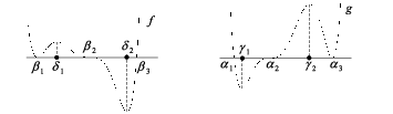
Figure 4. Real graphs of ff and gg (Example 4.3)
Refer to caption
Figure 5. Graph Σ\Sigma (Example 4.3)
Refer to caption
Figure 6. Bifurcation graph Γ\Gamma (Example 4.3)
Refer to caption
Figure 7. Satellites Γ⁡(−1)\Gamma(-1), Γ⁡(0)\Gamma(0) and Γ⁡(1)\Gamma(1) (Example 4.3)
Example 4.3.

Consider the ℝ\mathbb{R}-join-type curve CC defined by the polynomials f⁡(y)=(y+1)2​y3​(y−2)f(y)=(y+1)^{2}y^{3}(y-2) and g⁡(x)=2​(x+1)​x3​(x−1)2g(x)=2(x+1)x^{3}(x-1)^{2}. Then, ff has four critical points β1=−1\beta_{1}=-1, δ1=(1−5)/2\delta_{1}=(1-\sqrt{5})/2, β2=0\beta_{2}=0 and δ2=(1+5)/2\delta_{2}=(1+\sqrt{5})/2. The polynomial gg also has four critical points γ1=−(1+73)/12\gamma_{1}=-(1+\sqrt{73})/12, α2=0\alpha_{2}=0, γ2=−(1−73)/12\gamma_{2}=-(1-\sqrt{73})/12 and α3=1\alpha_{3}=1. See Figure 4. (In the figure, the numerical scale is not respected; however, the order f⁡(δ2)<g⁡(γ1)<f⁡(δ1)<g⁡(γ2)f(\delta_{2})<g(\gamma_{1})<f(\delta_{1})<g(\gamma_{2}) is rigorously respected.) As g⁡(γi)≠f⁡(δj)g(\gamma_{i})\not=f(\delta_{j}) for any 1≤i,j≤21\leq i,j\leq 2, the curve CC is generic. The corresponding graphs Σ\Sigma and Γ\Gamma are given in Figures 5 and 6 respectively. The satellites Γ⁡(−1)\Gamma(-1), Γ⁡(0)\Gamma(0) and Γ⁡(1)\Gamma(1) associated with Γ\Gamma are given in Figure 7. The black vertices and the full lines of the bifurcation graph Γ\Gamma correspond to the part above the positive branch Σ+\Sigma_{+} of Σ\Sigma. The white vertices and the dotted lines correspond to the part above the negative branch Σ−\Sigma_{-}. The star-style vertices represent the points α1=−1\alpha_{1}=-1, α2=0\alpha_{2}=0 and α3=1\alpha_{3}=1 which are the centres of the satellites. All the vertices (black, white and star-style) surrounded with a gray circle correspond to the special lines of the pencil 𝒫\mathscr{P}. As the curve is generic, we have π1​(ℂ2∖C)≃G⁡(1,1)≃ℤ\pi_{1}(\mathbb{C}^{2}\setminus C)\simeq G(1;1)\simeq\mathbb{Z} and π1​(ℙ2∖C~)≃G⁡(1,1,6)≃ℤ6\pi_{1}(\mathbb{P}^{2}\setminus\widetilde{C})\simeq G(1;1;6)\simeq\mathbb{Z}_{6} (by [2] or Theorem 1.3 above).

Now, let us give an example with a semi-generic curve which is not generic.

Example 4.4.

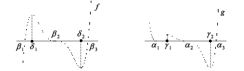
Consider the ℝ\mathbb{R}-join-type curve CC defined by the polynomials f⁡(y)=c⁡(y+1)​y3​(y−1)f(y)=c(y+1)y^{3}(y-1) and g⁡(x)=(x+1)2​x3​(x−2)g(x)=(x+1)^{2}x^{3}(x-2), where the coefficient cc is positive. We check easily that ff has three critical points δ1<β2=0<δ2\delta_{1}<\beta_{2}=0<\delta_{2}, while the polynomial gg has four critical points α1=−1<γ1<α2=0<γ2\alpha_{1}=-1<\gamma_{1}<\alpha_{2}=0<\gamma_{2}. We choose the coefficient cc so that f⁡(δ2)=g⁡(γ2)f(\delta_{2})=g(\gamma_{2}) (in particular, CC is not generic). See Figure 8. (Again, the figure is not numerically correct but the order f⁡(δ2)=g⁡(γ2)<g⁡(γ1)<f⁡(δ1)f(\delta_{2})=g(\gamma_{2})<g(\gamma_{1})<f(\delta_{1}) is respected.) Now, as g⁡(γ1)g(\gamma_{1}) is a regular value for ff, the satellite Γ⁡(α1)\Gamma(\alpha_{1}) is regular, and therefore the curve CC is semi-generic with respect to gg. The corresponding graphs Σ\Sigma and Γ\Gamma are given in Figures 9 and 10 respectively. The satellites Γ⁡(−1)\Gamma(-1), Γ⁡(0)\Gamma(0) and Γ⁡(2)\Gamma(2) associated with Γ\Gamma are given in Figure 11. (The significance of the colours is as above.) As the curve is semi-generic with respect to gg, Theorem 1.3 says that π1​(ℂ2∖C)≃G⁡(1,1)≃ℤ\pi_{1}(\mathbb{C}^{2}\setminus C)\simeq G(1;1)\simeq\mathbb{Z} and π1​(ℙ2∖C~)≃G⁡(1,1,6)≃ℤ6\pi_{1}(\mathbb{P}^{2}\setminus\widetilde{C})\simeq G(1;1;6)\simeq\mathbb{Z}_{6}.

Refer to caption
Figure 8. Real graphs of ff and gg (Example 4.4)
Refer to caption
Figure 9. Graph Σ\Sigma (Example 4.4)
Refer to caption
Figure 10. Bifurcation graph Γ\Gamma (Example 4.4)
Refer to caption
Figure 11. Satellites Γ⁡(−1)\Gamma(-1), Γ⁡(0)\Gamma(0) and Γ⁡(2)\Gamma(2) (Example 4.4)

5. Proof of Theorem 1.3

We suppose that CC has at least one exceptional singularity. (When CC is generic, the result is already proved in [2].) For simplicity, we shall assume v−<0v_{-}<0 and v+>0v_{+}>0, so that each satellite Γ⁡(αi)\Gamma(\alpha_{i}) (1≤i≤m1\leq i\leq m) has 2​λi2\lambda_{i} branches. (The proof can be easily adapted if v−=0v_{-}=0 or v+=0v_{+}=0.) As the curve is semi-generic with respect to gg, there exists i0i_{0} such that Γ⁡(αi0)\Gamma(\alpha_{i_{0}}) is a regular satellite (i.e., g⁡(γi0−1)∉𝒱crit​(f)g(\gamma_{i_{0}-1})\notin\mathscr{V}_{\mbox{\tiny crit}}(f) and g⁡(γi0)∉𝒱crit​(f)g(\gamma_{i_{0}})\notin\mathscr{V}_{\mbox{\tiny crit}}(f)).

As mentioned above, we use the Zariski–van Kampen theorem with the pencil 𝒫\mathscr{P} given by the vertical lines Lγ:x=γL_{\gamma}\colon x=\gamma, where γ∈ℂ\gamma\in\mathbb{C}. We take a sufficiently small positive number ε\varepsilon, and for any real number η\eta, we write η−:=η−ε\eta^{-}:=\eta-\varepsilon and η+:=η+ε\eta^{+}:=\eta+\varepsilon. We consider the generic line Lαi0+L_{\alpha_{i_{0}}^{+}}, and we choose generators

ξ1,0,…,ξ1,ν1−1,…,ξℓ,0,…,ξℓ,νℓ−1\xi_{1,0},\ldots,\xi_{1,\nu_{1}-1},\ldots,\xi_{\ell,0},\ldots,\xi_{\ell,\nu_{\ell}-1}

of the fundamental group π1​(Lαi0+∖C)\pi_{1}(L_{\alpha_{i_{0}}^{+}}\setminus C) as in Figure 12. (In the figure, we do not respect the numerical scale; we even zoom on the part that collapses to βj\beta_{j} when ε→0\varepsilon\rightarrow 0.) Here, the loops ξj,rj\xi_{j,r_{j}} (1≤j≤ℓ1\leq j\leq\ell, 0≤rj≤νj−10\leq r_{j}\leq\nu_{j}-1) are counterclockwise-oriented lassos around the intersection points of Lαi0+L_{\alpha_{i_{0}}^{+}} with CC. We shall refer to these generators as geometric generators.

Refer to caption
Figure 12. Generators of π1​(Lαi0+∖C)\pi_{1}(L_{\alpha_{i_{0}}^{+}}\setminus C)

For 1≤j≤ℓ1\leq j\leq\ell, 0≤rj≤νj−10\leq r_{j}\leq\nu_{j}-1 and n∈ℤn\in\mathbb{Z}, let

ωj:=ξj,νj−1​…​ξj,0andξj,n​νj+rj:=ωjn⋅ξj,rj⋅ωj−n.\displaystyle\omega_{j}:=\xi_{j,\nu_{j}-1}\ldots\xi_{j,0}\quad\mbox{and}\quad\xi_{j,n\nu_{j}+r_{j}}:=\omega_{j}^{n}\cdot\xi_{j,r_{j}}\cdot\omega_{j}^{-n}.

These relations define elements ξj,k\xi_{j,k} for any 1≤j≤ℓ1\leq j\leq\ell and any k∈ℤk\in\mathbb{Z}. (Indeed, any k∈ℤk\in\mathbb{Z} can be written as k=n​νj+rjk=n\nu_{j}+r_{j}, with n∈ℤn\in\mathbb{Z} and 0≤rj≤νj−10\leq r_{j}\leq\nu_{j}-1.) It is easy to see that

(5.1) ξj,n​νj+r=ωjn⋅ξj,r⋅ωj−nfor1≤j≤ℓ​ and ​n,r∈ℤ.\xi_{j,n\nu_{j}+r}=\omega_{j}^{n}\cdot\xi_{j,r}\cdot\omega_{j}^{-n}\quad\mbox{for}\quad 1\leq j\leq\ell\mbox{ and }n,r\in\mathbb{Z}.
Refer to caption
Figure 13. Example of standard generators of π1​(ℂ∖𝒮)\pi_{1}(\mathbb{C}\setminus\mathscr{S})

As usual, to find the monodromy relations associated with the special lines of the pencil 𝒫\mathscr{P}, we consider a ‘standard’ system of counterclockwise-oriented generators of the fundamental group π1​(ℂ∖𝒮)\pi_{1}(\mathbb{C}\setminus\mathscr{S}), where 𝒮\mathscr{S} is the set consisting of the vertices αi\alpha_{i} (1≤i≤m1\leq i\leq m) and γj,k\gamma_{j,k} (1≤j≤ℓ−11\leq j\leq\ell-1, 1≤k≤d′1\leq k\leq d^{\prime}) in the bifurcation graph Γ\Gamma. (We recall that the elements γj,k\gamma_{j,k} are the roots of the equation g⁡(x)=f⁡(δj)g(x)=f(\delta_{j}), where δj\delta_{j} is defined as in Section 1.) We choose αi0+\alpha_{i_{0}}^{+} as base point, and we denote these generators by σ⁡(αi)\sigma(\alpha_{i}) and σ⁡(γj,k)\sigma(\gamma_{j,k}). Then, σ⁡(αi)\sigma(\alpha_{i}) (respectively, σ⁡(γj,k)\sigma(\gamma_{j,k})) is a loop in ℂ∖𝒮\mathbb{C}\setminus\mathscr{S} surrounding the vertex αi\alpha_{i} (respectively, γj,k\gamma_{j,k}). It is based at αi0+\alpha_{i_{0}}^{+} and it runs along the edges of Γ\Gamma avoiding the vertices corresponding to special lines (cf. Figure 13). The monodromy relations around the special line LαiL_{\alpha_{i}} (respectively, Lγj,kL_{\gamma_{j,k}}) are obtained by moving the generic fibre Lαi0+∖CL_{\alpha_{i_{0}}^{+}}\setminus C isotopically ‘above’ the loop σ⁡(αi)\sigma(\alpha_{i}) (respectively, σ⁡(γj,k)\sigma(\gamma_{j,k})) and by identifying each generator ξj,rj\xi_{j,r_{j}} (1≤j≤ℓ1\leq j\leq\ell, 0≤rj≤νj−10\leq r_{j}\leq\nu_{j}-1) of the group π1​(Lαi0+∖C)\pi_{1}(L_{\alpha_{i_{0}}^{+}}\setminus C) with its image by the terminal homeomorphism of this isotopy (cf. [1, 4, 7]).

We start with the monodromy relations associated with the special line Lαi0L_{\alpha_{i_{0}}}. These relations can be found using the local models yνj=xλi0y^{\nu_{j}}=x^{\lambda_{i_{0}}} (1≤j≤ℓ1\leq j\leq\ell). Precisely, if we write λi0=nj​νj+rj\lambda_{i_{0}}=n_{j}\nu_{j}+r_{j}, nj∈ℤn_{j}\in\mathbb{Z}, 0≤rj≤νj−10\leq r_{j}\leq\nu_{j}-1, they are given by

{ξj,0=ωjnj⋅ξj,rj⋅ωj−nj,ξj,1=ωjnj⋅ξj,rj+1⋅ωj−nj,…ξj,νj−(rj+1)=ωjnj⋅ξj,νj−1⋅ωj−nj,ξj,νj−rj=ωjnj+1⋅ξj,0⋅ωj−(nj+1),…ξj,νj−1=ωjnj+1⋅ξj,rj−1⋅ωj−(nj+1).\left\{\begin{aligned} &\xi_{j,0}=\omega_{j}^{n_{j}}\cdot\xi_{j,r_{j}}\cdot\omega_{j}^{-n_{j}},\\ &\xi_{j,1}=\omega_{j}^{n_{j}}\cdot\xi_{j,r_{j}+1}\cdot\omega_{j}^{-n_{j}},\\ &\ldots\\ &\xi_{j,\nu_{j}-(r_{j}+1)}=\omega_{j}^{n_{j}}\cdot\xi_{j,\nu_{j}-1}\cdot\omega_{j}^{-n_{j}},\\ &\xi_{j,\nu_{j}-r_{j}}=\omega_{j}^{n_{j}+1}\cdot\xi_{j,0}\cdot\omega_{j}^{-(n_{j}+1)},\\ &\ldots\\ &\xi_{j,\nu_{j}-1}=\omega_{j}^{n_{j}+1}\cdot\xi_{j,r_{j}-1}\cdot\omega_{j}^{-(n_{j}+1)}.\\ \end{aligned}\right.

By (5.1), these relations can be written more concisely as

ξj,kj=ωjnj⋅ξj,kj+rj⋅ωj−nj=ξj,kj+λi0for1≤j≤ℓ​ and ​0≤kj≤νj−1.\displaystyle\xi_{j,k_{j}}=\omega_{j}^{n_{j}}\cdot\xi_{j,k_{j}+r_{j}}\cdot\omega_{j}^{-n_{j}}=\xi_{j,k_{j}+\lambda_{i_{0}}}\quad\mbox{for}\quad 1\leq j\leq\ell\mbox{ and }0\leq k_{j}\leq\nu_{j}-1.

In fact, (5.1) shows that

(5.2) ξj,k=ξj,k+λi0for1≤j≤ℓ​ and ​k∈ℤ.\displaystyle\xi_{j,k}=\xi_{j,k+\lambda_{i_{0}}}\quad\mbox{for}\quad 1\leq j\leq\ell\mbox{ and }k\in\mathbb{Z}.
Remark 5.1.

If νj=1\nu_{j}=1 for all 1≤j≤ℓ1\leq j\leq\ell, then Lαi0L_{\alpha_{i_{0}}} is not a special line, and hence, the corresponding monodromy relations are trivial. However, it is clear that the relations (5.2) remain valid. (Indeed, in this case, ξj,k=ξj,0\xi_{j,k}=\xi_{j,0} for all k∈ℤk\in\mathbb{Z}.)

Next, we look for the monodromy relations along the branches of Γ⁡(αi0)\Gamma(\alpha_{i_{0}}). For 0≤q≤2​λi0−10\leq q\leq 2\lambda_{i_{0}}-1, we denote by Bi0,qB_{i_{0},q} the qq-th branch of Γ⁡(αi0)\Gamma(\alpha_{i_{0}}). We suppose that the branches Bi0,2​qB_{i_{0},2q} (respectively, Bi0,2​q+1B_{i_{0},2q+1}), 0≤q≤λi0−10\leq q\leq\lambda_{i_{0}}-1, correspond to the positive part Σ+\Sigma_{+} (respectively, the negative part Σ−\Sigma_{-}) of Σ\Sigma through the correspondence Γ⁡(αi0)→Σ\Gamma(\alpha_{i_{0}})\to\Sigma given by the restriction of gg. We also suppose that the branch Bi0,0B_{i_{0},0} (respectively, Bi0,1B_{i_{0},1}) contains the line segment [αi0,γi0][\alpha_{i_{0}},\gamma_{i_{0}}] if g⁡(γi0)>0g(\gamma_{i_{0}})>0 (respectively, if g⁡(γi0)<0g(\gamma_{i_{0}})<0). For instance, in the special case of the satellite Γ⁡(α2)=Γ⁡(0)\Gamma(\alpha_{2})=\Gamma(0) of Example 4.3, the branches B2,qB_{2,q} are as in Figure 14. For simplicity, hereafter we shall suppose g⁡(γi0)>0g(\gamma_{i_{0}})>0. (The argument is similar in the case g⁡(γi0)<0g(\gamma_{i_{0}})<0.)

Refer to caption
Figure 14. Branches of the satellite Γ⁡(α2)\Gamma(\alpha_{2}) of Example 4.3
Refer to caption
Figure 15. Real graphs of ff and gg when 0<f⁡(δj0)<g⁡(γi0)0<f(\delta_{j_{0}})<g(\gamma_{i_{0}})
Refer to caption
Figure 16. Generators at x=αi0+x=\alpha_{i_{0}}^{+} (left-side) and at x=γi0,j0,0−x=\gamma_{i_{0},j_{0},0}^{-} (right-side) when g⁡(γi0)>0g(\gamma_{i_{0}})>0 and f⁡(δj0)>0f(\delta_{j_{0}})>0

Pick an element j0j_{0} such that 1≤j0≤ℓ−11\leq j_{0}\leq\ell-1. If f⁡(δj0)>0f(\delta_{j_{0}})>0, then, for each 0≤q≤λi0−10\leq q\leq\lambda_{i_{0}}-1, there exists an unique vertex γi0,j0,2​q∈Bi0,2​q\gamma_{i_{0},j_{0},2q}\in B_{i_{0},2q} such that g⁡(γi0,j0,2​q)=f⁡(δj0)g(\gamma_{i_{0},j_{0},2q})=f(\delta_{j_{0}}). For instance, in the special case of the satellite Γ⁡(α2)=Γ⁡(0)\Gamma(\alpha_{2})=\Gamma(0) of Example 4.3, f⁡(δ1)>0f(\delta_{1})>0 and for 0≤q≤20\leq q\leq 2 there exists an unique vertex γ2,1,2​q∈B2,2​q\gamma_{2,1,2q}\in B_{2,2q} such that g⁡(γ2,1,2​q)=f⁡(δ1)g(\gamma_{2,1,2q})=f(\delta_{1}) (cf. Figure 14). As Γ⁡(αi0)\Gamma(\alpha_{i_{0}}) is a regular satellite, g⁡(γi0)≠f⁡(δj0)g(\gamma_{i_{0}})\not=f(\delta_{j_{0}}), and hence γi0,j0,0≠γi0\gamma_{i_{0},j_{0},0}\not=\gamma_{i_{0}}. It follows that the monodromy relation associated with the line Lγi0,j0,0L_{\gamma_{i_{0},j_{0},0}} is a simple tangent relation (cf. (3.1)). Precisely, this relation is given by

(5.3) ξj0,0=ξj0+1,kj0,\displaystyle\xi_{j_{0},0}=\xi_{j_{0}+1,k_{j_{0}}},

where kj0k_{j_{0}} is some integer depending only on the first ordering of the elements ξj0+1,rj0+1\xi_{j_{0}+1,r_{j_{0}+1}}, 0≤rj0+1≤νj0+1−10\leq r_{j_{0}+1}\leq\nu_{j_{0}+1}-1 (cf. Figures 15 and 16). The graphs in Figure 15 are the real graphs of ff and gg in neighbourhoods of the intervals [αi0,αi0+1][\alpha_{i_{0}},\alpha_{i_{0}+1}] and [βj0,βj0+1][\beta_{j_{0}},\beta_{j_{0}+1}], respectively; c⁡(ξj0,0)c(\xi_{j_{0},0}) and c⁡(ξj0+1,kj0)c(\xi_{j_{0}+1,k_{j_{0}}}) are the centres of the lassos ξj0,0\xi_{j_{0},0} and ξj0+1,kj0\xi_{j_{0}+1,k_{j_{0}}}, respectively. The picture on the left-side (respectively, right-side) of Figure 16 represents the generators in a neighbourhood of βj0\beta_{j_{0}} and βj0+1\beta_{j_{0}+1} (respectively, in a neighbourhood of δj0\delta_{j_{0}}) at x=αi0+x=\alpha_{i_{0}}^{+} (respectively, at x=γi0,j0,0−x=\gamma_{i_{0},j_{0},0}^{-}).

Actually, as Γ⁡(αi0)\Gamma(\alpha_{i_{0}}) is regular, γi0,j0,2​q∉{γi0−1,γi0}\gamma_{i_{0},j_{0},2q}\notin\{\gamma_{i_{0}-1},\gamma_{i_{0}}\} for any 0≤q≤λi0−10\leq q\leq\lambda_{i_{0}}-1, and the monodromy relation associated with the special line Lγi0,j0,2​qL_{\gamma_{i_{0},j_{0},2q}} is a simple tangent relation given by

(5.4) ξj0,−q=ξj0+1,kj0−q.\displaystyle\xi_{j_{0},-q}=\xi_{j_{0}+1,k_{j_{0}}-q}.

This follows immediately from (5.3) and the following observation.

Observation 5.2.

For any ii (1≤i≤m1\leq i\leq m), when xx moves on the circle |x−αi|=ε|x-\alpha_{i}|=\varepsilon by the angle 2​π/λi2\pi/\lambda_{i}, the centre of each lasso ξj,rj\xi_{j,r_{j}} (1≤j≤ℓ1\leq j\leq\ell, 0≤rj≤νj−10\leq r_{j}\leq\nu_{j}-1) turns on the circle |y−βj|=ελi/νj|y-\beta_{j}|=\varepsilon^{\lambda_{i}/\nu_{j}} by the angle 2​π/νj2\pi/\nu_{j}.

Similarly, if f⁡(δj0)<0f(\delta_{j_{0}})<0, then, for each 0≤q≤λi0−10\leq q\leq\lambda_{i_{0}}-1, there exists an unique vertex γi0,j0,2​q+1∈Bi0,2​q+1\gamma_{i_{0},j_{0},2q+1}\in B_{i_{0},2q+1} such that g⁡(γi0,j0,2​q+1)=f⁡(δj0)g(\gamma_{i_{0},j_{0},2q+1})=f(\delta_{j_{0}}), and by the same argument as above, the monodromy relation associated with the line Lγi0,j0,2​q+1L_{\gamma_{i_{0},j_{0},2q+1}} is given by

(5.5) ξj0,hj0−q=ξj0+1,kj0−q,\displaystyle\xi_{j_{0},h_{j_{0}}-q}=\xi_{j_{0}+1,k_{j_{0}}-q},

where hj0h_{j_{0}} and kj0k_{j_{0}} are integers depending only on the first ordering of the elements ξj0,rj0\xi_{j_{0},r_{j_{0}}} (0≤rj0≤νj0−10\leq r_{j_{0}}\leq\nu_{j_{0}}-1) and ξj0+1,rj0+1\xi_{j_{0}+1,r_{j_{0}+1}} (0≤rj0+1≤νj0+1−10\leq r_{j_{0}+1}\leq\nu_{j_{0}+1}-1).

Remark 5.3.

Note that the relations (5.4) can also be written under the form (5.5) by taking hj0=0h_{j_{0}}=0.

Combined with (5.2), the relations (5.5) imply

ξj0,hj0−k=ξj0+1,kj0−kfork∈ℤ,\displaystyle\xi_{j_{0},h_{j_{0}}-k}=\xi_{j_{0}+1,k_{j_{0}}-k}\quad\mbox{for}\quad k\in\mathbb{Z},

and therefore,

ξj0,k=ξj0+1,k+(kj0−hj0)fork∈ℤ.\displaystyle\xi_{j_{0},k}=\xi_{j_{0}+1,k+(k_{j_{0}}-h_{j_{0}})}\quad\mbox{for}\quad k\in\mathbb{Z}.

Then, by reordering the generators ξj,k\xi_{j,k} successively for j=2,…,ℓj=2,\ldots,\ell, we can assume that

(5.6) ξj0,k=ξj0+1,kfork∈ℤ,\displaystyle\xi_{j_{0},k}=\xi_{j_{0}+1,k}\quad\mbox{for}\quad k\in\mathbb{Z},

and hence, as j0j_{0} is arbitrary, we can take, as generators, the elements

(5.7) ξk:=ξj0,kfork∈ℤ.\displaystyle\xi_{k}:=\xi_{j_{0},k}\quad\mbox{for}\quad k\in\mathbb{Z}.

Then, the relations (5.2) are written as

(5.8) ξk=ξk+λi0fork∈ℤ,\displaystyle\xi_{k}=\xi_{k+\lambda_{i_{0}}}\quad\mbox{for}\quad k\in\mathbb{Z},

and, by applying Proposition 2.2, we have

(5.9) ξk+ν0=ω​ξk​ω−1fork∈ℤ,\displaystyle\xi_{k+\nu_{0}}=\omega\xi_{k}\omega^{-1}\quad\mbox{for}\quad k\in\mathbb{Z},

where ω:=ξν0−1​…​ξ0\omega:=\xi_{\nu_{0}-1}\ldots\xi_{0}. Indeed, by Bezout’s identity, there exist k1,…,kℓ∈ℤk_{1},\ldots,k_{\ell}\in\mathbb{Z} such that ν0=k1​ν1+…+kℓ​νℓ\nu_{0}=k_{1}\nu_{1}+\ldots+k_{\ell}\nu_{\ell}. Then, by (5.1),

ξk+ν0=(ωℓkℓ​…​ω1k1)⋅ξk⋅(ωℓkℓ​…​ω1k1)−1,\xi_{k+\nu_{0}}=(\omega_{\ell}^{k_{\ell}}\ldots\omega_{1}^{k_{1}})\cdot\xi_{k}\cdot(\omega_{\ell}^{k_{\ell}}\ldots\omega_{1}^{k_{1}})^{-1},

while Proposition 2.2 shows that

ωℓkℓ​…​ω1k1=ξν0−1​…​ξ0.\omega_{\ell}^{k_{\ell}}\ldots\omega_{1}^{k_{1}}=\xi_{\nu_{0}-1}\ldots\xi_{0}.
Remark 5.4.

The relations (5.8) and (5.9) associated with the regular satellite Γ⁡(αi0)\Gamma(\alpha_{i_{0}}) imply that the fundamental group π1​(ℂ2∖C)\pi_{1}({\mathbb{C}^{2}\setminus C}) is a quotient of the group G⁡(ν0,λi0)G(\nu_{0};\lambda_{i_{0}}).

Refer to caption
Figure 17. The modified line segment (αi0+,αi0+1−)(\alpha_{i_{0}}^{+},\alpha_{i_{0}+1}^{-})
Refer to caption
Figure 18. Deformation of the generators when 0<f⁡(δj0)<g⁡(γi0)0<f(\delta_{j_{0}})<g(\gamma_{i_{0}})

Now, let us consider the monodromy relations associated with the other satellites. For simplicity, we still assume g⁡(γi0)>0g(\gamma_{i_{0}})>0. We start with the satellite Γ⁡(αi0+1)\Gamma(\alpha_{i_{0}+1}) and first look for the relations around the line Lαi0+1L_{\alpha_{i_{0}+1}}. For this purpose, we need to know how the generators are deformed when xx moves along the ‘modified’ line segment (αi0+,αi0+1−)(\alpha_{i_{0}}^{+},\alpha_{i_{0}+1}^{-}). Here, ‘modified’ means that xx makes a half-turn counterclockwise around each vertex of Γ∩(αi0+,αi0+1−)\Gamma\cap(\alpha_{i_{0}}^{+},\alpha_{i_{0}+1}^{-}) corresponding to a special line (cf. Figure 17). Take an element j0j_{0} such that 1≤j0≤ℓ−11\leq j_{0}\leq\ell-1. If 0<f⁡(δj0)<g⁡(γi0)0<f(\delta_{j_{0}})<g(\gamma_{i_{0}}), then there are exactly two vertices γi0,j0,0≠γi0\gamma_{i_{0},j_{0},0}\not=\gamma_{i_{0}} and γi0+1,j0,2​q0≠γi0\gamma_{i_{0}+1,j_{0},2q_{0}}\not=\gamma_{i_{0}} (for some 0≤q0≤λi0+1−10\leq q_{0}\leq\lambda_{i_{0}+1}-1) on the line segment (αi0+,αi0+1−)(\alpha_{i_{0}}^{+},\alpha_{i_{0}+1}^{-}) that correspond to the special lines of the pencil associated with the critical value f⁡(δj0)f(\delta_{j_{0}}) (i.e., g⁡(γi0,j0,0)=f⁡(δj0)g(\gamma_{i_{0},j_{0},0})=f(\delta_{j_{0}}) and g⁡(γi0+1,j0,2​q0)=f⁡(δj0)g(\gamma_{i_{0}+1,j_{0},2q_{0}})=f(\delta_{j_{0}})). The first one γi0,j0,0\gamma_{i_{0},j_{0},0} is in Γ⁡(αi0)\Gamma(\alpha_{i_{0}}) and the second one γi0+1,j0,2​q0\gamma_{i_{0}+1,j_{0},2q_{0}} is in Γ⁡(αi0+1)\Gamma(\alpha_{i_{0}+1}). Therefore, when xx moves along the modified line segment (αi0+,αi0+1−)(\alpha_{i_{0}}^{+},\alpha_{i_{0}+1}^{-}), the generators are deformed as in Figure 18. The picture on the left-side of the figure represents the generators at x=αi0+x=\alpha_{i_{0}}^{+} (i.e., before the deformation). The picture on the right-side represents the generators at x=αi0+1−x=\alpha_{i_{0}+1}^{-} (i.e., after the deformation). However, by (5.6), we can suppose that the generators in the fibre x=αi0+1−x=\alpha_{i_{0}+1}^{-} are still the same as in the fibre x=αi0+x=\alpha_{i_{0}}^{+}. In other words, the picture on the left-side of Figure 18 also represents the generators at x=αi0+1−x=\alpha_{i_{0}+1}^{-}. Hence, by the same argument as above, the monodromy relations associated with the special line Lαi0+1L_{\alpha_{i_{0}+1}} give the relations

(5.10) ξk=ξk+λi0+1fork∈ℤ.\displaystyle\xi_{k}=\xi_{k+\lambda_{i_{0}+1}}\quad\mbox{for}\quad k\in\mathbb{Z}.

We get the same relations if g⁡(γi0)<f⁡(δj0)g(\gamma_{i_{0}})<f(\delta_{j_{0}}) or if f⁡(δj0)<0f(\delta_{j_{0}})<0. Indeed, in these two cases, the set g−1​(f⁡(δj0))∩(αi0+,αi0+1−)g^{-1}(f(\delta_{j_{0}}))\cap(\alpha_{i_{0}}^{+},\alpha_{i_{0}+1}^{-}) is empty, and therefore the configuration of the generators is identical on the fibres x=αi0+1−x=\alpha_{i_{0}+1}^{-} and x=αi0+x=\alpha_{i_{0}}^{+}.

Refer to caption
Figure 19. Generators at x=αi0+1+x=\alpha_{i_{0}+1}^{+} and x=αi0+2−x=\alpha_{i_{0}+2}^{-} when g⁡(γi0)g(\gamma_{i_{0}}), g⁡(γi0+1)g(\gamma_{i_{0}+1}) and f⁡(δj0)f(\delta_{j_{0}}) are >0>0

The monodromy relations around the special lines corresponding to the vertices located on the branches of Γ⁡(αi0+1)\Gamma(\alpha_{i_{0}+1}) do not give any new relation. This can be directly shown easily but it is not necessary. In fact, as we shall see below, it suffices to collect the monodromy relations associated with the special lines LαiL_{\alpha_{i}} for all ii, 1≤i≤m1\leq i\leq m. We already know that, for i=i0i=i_{0} and i0+1i_{0}+1, the monodromy relations around LαiL_{\alpha_{i}} are given by ξk=ξk+λi\xi_{k}=\xi_{k+\lambda_{i}} for all k∈ℤk\in\mathbb{Z}. In fact, this is true for any ii. For instance, let us show it for i=i0+2i=i_{0}+2. For this purpose, we need to know how the generators are deformed when xx makes a half-turn on the circle |x−αi0+1|=ε|x-\alpha_{i_{0}+1}|=\varepsilon from αi0+1−\alpha_{i_{0}+1}^{-} to αi0+1+\alpha_{i_{0}+1}^{+}, and then moves along the modified line segment (αi0+1+,αi0+2−)(\alpha_{i_{0}+1}^{+},\alpha_{i_{0}+2}^{-}). Again, take j0j_{0} such that 1≤j0≤ℓ−11\leq j_{0}\leq\ell-1, and for simplicity assume that g⁡(γi0)g(\gamma_{i_{0}}), g⁡(γi0+1)g(\gamma_{i_{0}+1}) and f⁡(δj0)f(\delta_{j_{0}}) are positive. (The other cases are similar and left to the reader.) By Observation 5.2, when xx makes a half-turn on the circle |x−αi0+1|=ε|x-\alpha_{i_{0}+1}|=\varepsilon from αi0+1−\alpha_{i_{0}+1}^{-} to αi0+1+\alpha_{i_{0}+1}^{+}, the generators are deformed as in Figure 19, where k0′∈ℤk^{\prime}_{0}\in\mathbb{Z}. That is, the configuration of the generators on the fibre x=αi0+1+x=\alpha_{i_{0}+1}^{+} is just the parallel translation of that on the fibre x=αi0+1−x=\alpha_{i_{0}+1}^{-}. When xx moves along the modified line segment (αi0+1+,αi0+2−)(\alpha_{i_{0}+1}^{+},\alpha_{i_{0}+2}^{-}), the generators are still as in Figure 19. The proof of this fact is as above except that now γi0+1∈(αi0+1+,αi0+2−)\gamma_{i_{0}+1}\in(\alpha_{i_{0}+1}^{+},\alpha_{i_{0}+2}^{-}) may correspond to an exceptional singularity (in particular, we may have f⁡(δj0)=g⁡(γi0+1)f(\delta_{j_{0}})=g(\gamma_{i_{0}+1})). But in this case, when xx makes a half-turn on the circle |x−γi0+1|=ε|x-\gamma_{i_{0}+1}|=\varepsilon from γi0+1−\gamma_{i_{0}+1}^{-} to γi0+1+\gamma_{i_{0}+1}^{+}, the generators remains unchanged, as, by (5.6), ξj0,k0′=ξj0+1,k0′\xi_{j_{0},k^{\prime}_{0}}=\xi_{j_{0}+1,k^{\prime}_{0}}. Finally, exactly as above, the monodromy relations associated with the special line Lαi0+2L_{\alpha_{i_{0}+2}} give the relations

ξk=ξk+λi0+2fork∈ℤ.\displaystyle\xi_{k}=\xi_{k+\lambda_{i_{0}+2}}\quad\mbox{for}\quad k\in\mathbb{Z}.

This argument can be repeated for all the other values of ii, 1≤i≤m1\leq i\leq m, so that the monodromy relations associated with the special line LαiL_{\alpha_{i}} for any ii, 1≤i≤m1\leq i\leq m, are written as

(5.11) ξk=ξk+λifork∈ℤ.\displaystyle\xi_{k}=\xi_{k+\lambda_{i}}\quad\mbox{for}\quad k\in\mathbb{Z}.

By Proposition 2.3, the collection of relations (5.11), for 1≤i≤m1\leq i\leq m, and the relation (5.9) are equivalent to

{ξk=ξk+λ0ξk+ν0=ω​ξk​ω−1fork∈ℤ.\left\{\begin{aligned} &\xi_{k}=\xi_{k+\lambda_{0}}\\ &\xi_{k+\nu_{0}}=\omega\xi_{k}\omega^{-1}\end{aligned}\right.\quad\mbox{for}\quad k\in\mathbb{Z}.

In particular, this means that the fundamental group π1​(ℂ2∖C)\pi_{1}(\mathbb{C}^{2}\setminus C) is presented by the generators ξk\xi_{k} (k∈ℤk\in\mathbb{Z}) and ω\omega and by a set of relations that includes the following relations:

(5.12) ω=ξν0−1​…​ξ0,\displaystyle\omega=\xi_{\nu_{0}-1}\ldots\xi_{0},
(5.13) ξk+λ0=ξk(k∈ℤ),\displaystyle\xi_{k+\lambda_{0}}=\xi_{k}\quad(k\in\mathbb{Z}),
(5.14) ξk+ν0=ω​ξk​ω−1(k∈ℤ).\displaystyle\xi_{k+\nu_{0}}=\omega\xi_{k}\omega^{-1}\quad(k\in\mathbb{Z}).

In other words, π1​(ℂ2∖C)\pi_{1}(\mathbb{C}^{2}\setminus C) is a quotient of the group G⁡(ν0,λ0)G(\nu_{0};\lambda_{0}).

Now, consider the family {Ct}0≤t≪1\{C_{t}\}_{0\leq t\ll 1} of ℝ\mathbb{R}-join type curves, where CtC_{t} is defined by the equation

f⁡(y)=(1−t)​g​(x).f(y)=(1-t)g(x).

For any 0<t≪10<t\ll 1, it is easy to see that the curve CtC_{t} has only inner singularities. Therefore, by the degeneration principle [5, 7], for any sufficiently small t>0t>0, there is a canonical epimorphism

ψt:π1​(ℂ2∖C)=π1​(ℂ2∖C0)↠π1​(ℂ2∖Ct)≃G⁡(ν0,λ0).\psi_{t}\colon\pi_{1}(\mathbb{C}^{2}\setminus C)=\pi_{1}(\mathbb{C}^{2}\setminus C_{0})\twoheadrightarrow\pi_{1}(\mathbb{C}^{2}\setminus C_{t})\simeq G(\nu_{0};\lambda_{0}).

Let us recall briefly how ψt\psi_{t} is defined. Let L∞L_{\infty} be the line at infinity, and set C′:=C∪L∞C^{\prime}:=C\cup L_{\infty} and Ct′:=Ct∪L∞C^{\prime}_{t}:=C_{t}\cup L_{\infty}. Pick a sufficiently small regular neighbourhood NN of C′C^{\prime} in ℙ2\mathbb{P}^{2} so that ı:ℙ2∖N↪ℙ2∖C′=ℂ2∖C\imath\colon\mathbb{P}^{2}\setminus N\hookrightarrow\mathbb{P}^{2}\setminus C^{\prime}=\mathbb{C}^{2}\setminus C is a homotopy equivalence, and take a sufficiently small tt so that Ct′C_{t}^{\prime} is contained in NN. Then, ψt\psi_{t} is defined by taking the composition of ı♯−1:π1​(ℂ2∖C)→π1​(ℙ2∖N){\imath_{\sharp}}^{-1}\colon\pi_{1}(\mathbb{C}^{2}\setminus C)\to\pi_{1}(\mathbb{P}^{2}\setminus N) with the homomorphism induced by the inclusion ℙ2∖N↪ℙ2∖Ct′=ℂ2∖Ct\mathbb{P}^{2}\setminus N\hookrightarrow\mathbb{P}^{2}\setminus C^{\prime}_{t}=\mathbb{C}^{2}\setminus C_{t}. To distinguish the generators, we write ξk​(t)\xi_{k}(t) (k∈ℤk\in\mathbb{Z}) for the generators of π1​(ℂ2∖Ct)\pi_{1}(\mathbb{C}^{2}\setminus C_{t}), which are represented by the same loops as ξk\xi_{k}. Note that ψt​(ξk)=ξk​(t)\psi_{t}(\xi_{k})=\xi_{k}(t). As CtC_{t} is generic, π1​(ℂ2∖Ct)\pi_{1}(\mathbb{C}^{2}\setminus C_{t}) is presented by the generators ξk​(t)\xi_{k}(t) (k∈ℤk\in\mathbb{Z}) and ω⁡(t):=ξν0−1​(t)​…​ξ0​(t)\omega(t):=\xi_{\nu_{0}-1}(t)\ldots\xi_{0}(t) and by the relations (5.12)–(5.14), replacing ξk\xi_{k} by ξk​(t)\xi_{k}(t) and ω\omega by ω⁡(t)\omega(t). (We may assume that N∩Lαi0+N\cap L_{\alpha_{i_{0}}^{+}} is a copy of dd disjoint (topologically) tiny 22-disks so that ξk\xi_{k} (0≤k≤d−10\leq k\leq d-1) are free generators of π1​(Lαi0+∖N)\pi_{1}(L_{\alpha_{i_{0}}^{+}}\setminus N).) This implies that ker⁡ψt\ker\psi_{t} is trivial, and hence

π1​(ℂ2∖C)≃G⁡(ν0,λ0).\pi_{1}(\mathbb{C}^{2}\setminus C)\simeq G(\nu_{0};\lambda_{0}).

(In particular, the branches of the satellites Γ⁡(αi)\Gamma(\alpha_{i}), i≠i0i\not=i_{0}, do not give any new relation.)

As for the fundamental group π1​(ℙ2∖C~)\pi_{1}(\mathbb{P}^{2}\setminus\widetilde{C}), we proceed as follows. If d≥d′d\geq d^{\prime}, then the base locus of the pencil X=γ​ZX=\gamma Z (γ∈ℂ\gamma\in\mathbb{C}) in ℙ2\mathbb{P}^{2} does not belong to the curve, and therefore the group π1​(ℙ2∖C~)\pi_{1}(\mathbb{P}^{2}\setminus\widetilde{C}) is obtained from the above presentation of π1​(ℂ2∖C)\pi_{1}(\mathbb{C}^{2}\setminus C) by adding the vanishing relation at infinity ω1​…​ωℓ=e\omega_{1}\ldots\omega_{\ell}=e. By Proposition 2.2, the relations (5.12) and (5.14) imply ωj=ωνj/ν0\omega_{j}=\omega^{\nu_{j}/\nu_{0}} (1≤j≤ℓ1\leq j\leq\ell). Therefore, the relation ω1​…​ωℓ=e\omega_{1}\ldots\omega_{\ell}=e can also be written as

ωd/ν0=e.\omega^{d/\nu_{0}}=e.

It follows that π1​(ℙ2∖C~)≃G⁡(ν0,λ0,d/ν0)\pi_{1}(\mathbb{P}^{2}\setminus\widetilde{C})\simeq G(\nu_{0};\lambda_{0};d/\nu_{0}).

If d′≥dd^{\prime}\geq d, then we consider again the family {Ct}0≤t≪1\{C_{t}\}_{0\leq t\ll 1}, where CtC_{t} is defined by the equation f⁡(y)=(1−t)​g​(x)f(y)=(1-t)g(x). We use the same regular neighbourhood NN and the same isomorphism ψt:π1​(ℂ2∖C)→π1​(ℂ2∖Ct)\psi_{t}\colon\pi_{1}(\mathbb{C}^{2}\setminus C)\to\pi_{1}(\mathbb{C}^{2}\setminus C_{t}) for a sufficiently small t>0t>0. To compute π1​(ℂ2∖C)\pi_{1}(\mathbb{C}^{2}\setminus C), this time we consider the pencil given by the horizontal lines y=δy=\delta, where δ∈ℂ\delta\in\mathbb{C}. We fix a generic line y=δ0y=\delta_{0} and we choose geometric generators ρk\rho_{k} (0≤k≤d′−10\leq k\leq d^{\prime}-1) as above so that the ρk\rho_{k}’s give generators of the fundamental group of the generic fibre of each complement ℙ2∖N\mathbb{P}^{2}\setminus N, ℂ2∖C\mathbb{C}^{2}\setminus C and ℂ2∖Ct\mathbb{C}^{2}\setminus C_{t} simultaneously. Then we define elements τ\tau and ρk\rho_{k}, for k∈ℤk\in\mathbb{Z}, in the same way as we defined the elements ω\omega and ξk\xi_{k} (k∈ℤk\in\mathbb{Z}) above. Now, as ψt\psi_{t} is an isomorphism and CtC_{t} is generic, the generating relations for each group π1​(ℂ2∖Ct)\pi_{1}(\mathbb{C}^{2}\setminus C_{t}), π1​(ℂ2∖C)\pi_{1}(\mathbb{C}^{2}\setminus C) and π1​(ℙ2∖N)\pi_{1}(\mathbb{P}^{2}\setminus N) are given by

τ=ρλ0−1​…​ρ0,\displaystyle\tau=\rho_{\lambda_{0}-1}\ldots\rho_{0},
ρk+ν0=ρk(k∈ℤ),\displaystyle\rho_{k+\nu_{0}}=\rho_{k}\quad(k\in\mathbb{Z}),
ρk+λ0=τ​ρk​τ−1(k∈ℤ).\displaystyle\rho_{k+\lambda_{0}}=\tau\rho_{k}\tau^{-1}\quad(k\in\mathbb{Z}).

As d′≥dd^{\prime}\geq d, the base locus of the pencil Y=δ​ZY=\delta Z (δ∈ℂ\delta\in\mathbb{C}) in ℙ2\mathbb{P}^{2} does not belong to C~\widetilde{C}, and hence the group π1​(ℙ2∖C~)\pi_{1}(\mathbb{P}^{2}\setminus\widetilde{C}) is obtained from the above presentation of π1​(ℂ2∖C)\pi_{1}(\mathbb{C}^{2}\setminus C) by adding the vanishing relation at infinity τd′/λ0=e\tau^{d^{\prime}/\lambda_{0}}=e. Finally, we get π1​(ℙ2∖C~)≃G⁡(λ0,ν0,d′/λ0)\pi_{1}(\mathbb{P}^{2}\setminus\widetilde{C})\simeq G(\lambda_{0};\nu_{0};d^{\prime}/\lambda_{0}).

6. Applications

In this section, we give two applications of Theorem 1.3.

6.1. Maximal irreducible nodal curves

An irreducible curve is said to be nodal if it has only node singularities. By Plücker’s formula, an irreducible nodal curve of degree dd has at most (d−1)​(d−2)/2(d-1)(d-2)/2 nodes. An irreducible nodal curve is called maximal if it has exactly (d−1)​(d−2)/2(d-1)(d-2)/2 nodes (equivalently, if its genus is 00). A method to construct such curves is given in [3]. There, the irreducibility is obtained using the braid group action. Hereafter, we repeat the construction of [3] but apply Theorem 1.3 to show the irreducibility.

For simplicity, let us suppose that d=2​n+1d=2n+1, n∈ℤn\in\mathbb{Z}. (The construction is similar when dd is even.) Consider the Chebyshev polynomial of degree dd, which is defined by Td​(z):=cos⁡(d​arccos⁡(z))T_{d}(z):=\cos(d\arccos(z)). This polynomial has 2​n+12n+1 simple real roots β1<…<β2​n+1\beta_{1}<\ldots<\beta_{2n+1} and 2​n2n critical points δ1,…,δ2​n\delta_{1},\ldots,\delta_{2n}, with δj∈(βj,βj+1)\delta_{j}\in(\beta_{j},\beta_{j+1}), such that Td​(δ1)=Td​(δ3)=…=Td​(δ2​n−1)=1T_{d}(\delta_{1})=T_{d}(\delta_{3})=\ldots=T_{d}(\delta_{2n-1})=1 and Td​(δ2)=Td​(δ4)=…=Td​(δ2​n)=−1T_{d}(\delta_{2})=T_{d}(\delta_{4})=\ldots=T_{d}(\delta_{2n})=-1. Now, take a small deformation T~d​(z)\widetilde{T}_{d}(z) of Td​(z)T_{d}(z) so that:

  1. (1)

    T~d​(z)\widetilde{T}_{d}(z) has nn critical points γ1,γ3,…,γ2​n−1\gamma_{1},\gamma_{3},\ldots,\gamma_{2n-1} such that T~d​(γ1)=T~d​(γ3)=…=T~d​(γ2​n−1)=1\widetilde{T}_{d}(\gamma_{1})=\widetilde{T}_{d}(\gamma_{3})=\ldots=\widetilde{T}_{d}(\gamma_{2n-1})=1;

  2. (2)

    T~d​(z)\widetilde{T}_{d}(z) has n−1n-1 critical points γ2,γ4,…,γ2​n−2\gamma_{2},\gamma_{4},\ldots,\gamma_{2n-2} such that T~d​(γ2)=T~d​(γ4)=…=T~d​(γ2​n−2)=−1\widetilde{T}_{d}(\gamma_{2})=\widetilde{T}_{d}(\gamma_{4})=\ldots=\widetilde{T}_{d}(\gamma_{2n-2})=-1;

  3. (3)

    T~d​(z)\widetilde{T}_{d}(z) has a critical point γ2​n\gamma_{2n} with T~d​(γ2​n)<−1\widetilde{T}_{d}(\gamma_{2n})<-1.

The existence of such a polynomial T~d​(z)\widetilde{T}_{d}(z) is due to R. Thom [6]. It has 2​n+12n+1 simple real roots α1<…<α2​n+1\alpha_{1}<\ldots<\alpha_{2n+1}, and γi∈(αi,αi+1)\gamma_{i}\in(\alpha_{i},\alpha_{i+1}). Then, consider the ℝ\mathbb{R}-join-type curve CC defined by Td​(y)=T~d​(x)T_{d}(y)=\widetilde{T}_{d}(x). Clearly, the satellite Γ⁡(α2​n+1)\Gamma(\alpha_{2n+1}) (of the bifurcation graph of CC with respect to T~d\widetilde{T}_{d}) is regular and the numbers ν0,λ0\nu_{0},\lambda_{0} which appear in Theorem 1.3 are equal to 11. Hence, π1​(ℂ2∖C)≃ℤ\pi_{1}(\mathbb{C}^{2}\setminus C)\simeq\mathbb{Z} and π1​(ℙ2∖C~)≃ℤd\pi_{1}(\mathbb{P}^{2}\setminus\widetilde{C})\simeq\mathbb{Z}_{d}. In particular, the curve CC is irreducible. The number of nodes is given by the cardinality of the set

{(γ2​i−1,δ2​j−1)∣1≤i,j≤n}∪{(γ2​i,δ2​j)∣1≤i≤n−1, 1≤j≤n},\displaystyle\{(\gamma_{2i-1},\delta_{2j-1})\mid 1\leq i,j\leq n\}\cup\{(\gamma_{2i},\delta_{2j})\mid 1\leq i\leq n-1,\,1\leq j\leq n\},

that is,

n2+(n−1)​n=(d−1)​(d−2)2.\displaystyle n^{2}+(n-1)n=\frac{(d-1)(d-2)}{2}.

In other words, CC is a maximal irreducible nodal curve.

6.2. Curves with node and cusp singularities

Let C:f⁡(y)=g⁡(x)C\colon f(y)=g(x) be an ℝ\mathbb{R}-join-type curve with only nodes and cusps as singularities. For simplicity, we suppose that CC has degree d=6​nd=6n, n∈ℤn\in\mathbb{Z}. The maximal number of cusps on such a curve is obtained when ff and gg have the form f⁡(y)=a​(y−β1)3​(y−β2)3​…​(y−β2​n)3f(y)=a(y-\beta_{1})^{3}(y-\beta_{2})^{3}\ldots(y-\beta_{2n})^{3} and g⁡(x)=b​(x−α1)2​(x−α2)2​…​(x−α3​n)2g(x)=b(x-\alpha_{1})^{2}(x-\alpha_{2})^{2}\ldots(x-\alpha_{3n})^{2}, in which case we have 6​n26n^{2} cusps. (As usual, we suppose βj<βj+1\beta_{j}<\beta_{j+1} and αi<αi+1\alpha_{i}<\alpha_{i+1} for all i,ji,j.) By the result of R. Thom [6], ff can be chosen so that its 2​n−12n-1 critical points δ1<…<δ2​n−1\delta_{1}<\ldots<\delta_{2n-1} satisfy f⁡(δ1)=f⁡(δ3)=…=f⁡(δ2​n−1)=−1f(\delta_{1})=f(\delta_{3})=\ldots=f(\delta_{2n-1})=-1 and f⁡(δ2)=f⁡(δ4)=…=f⁡(δ2​n−2)=1f(\delta_{2})=f(\delta_{4})=\ldots=f(\delta_{2n-2})=1. Similarly, gg can be chosen so that its 3​n−13n-1 critical points γ1<…<γ3​n−1\gamma_{1}<\ldots<\gamma_{3n-1} satisfy g⁡(γ1)=g⁡(γ2)=…=g⁡(γ3​n−2)=−1>g⁡(γ3​n−1)g(\gamma_{1})=g(\gamma_{2})=\ldots=g(\gamma_{3n-2})=-1>g(\gamma_{3n-1}). In this case, the curve also has n⁡(3​n−2)n(3n-2) nodes. Clearly, the satellite Γ⁡(α3​n)\Gamma(\alpha_{3n}) (of the bifurcation graph of CC with respect to gg) is regular, and hence, by Theorem 1.3, π1​(ℂ2∖C)≃G⁡(3,2)≃B⁡(3)\pi_{1}(\mathbb{C}^{2}\setminus C)\simeq G(3;2)\simeq B(3) (the braid group on 33 strings), while π1​(ℙ2∖C~)≃G⁡(3,2,2​n)\pi_{1}(\mathbb{P}^{2}\setminus\widetilde{C})\simeq G(3;2;2n). Note that, by Theorem (2.12) of [2], we have a central extension

0→ℤn→G⁡(3,2,2​n)→ℤ3∗ℤ2→0,0\rightarrow\mathbb{Z}_{n}\rightarrow G(3;2;2n)\rightarrow\mathbb{Z}_{3}*\mathbb{Z}_{2}\rightarrow 0,

where ℤn\mathbb{Z}_{n} is generated by ω2\omega^{2}.

References

  • [1] E. R. van Kampen, On the fundamental group of an algebraic curve, Amer. J. Math. 55 (1933) 255–260.
  • [2] M. Oka, On the fundamental group of the complement of certain plane curves, J. Math. Soc. Japan 30 (1978) 579–597.
  • [3] M. Oka, Symmetric plane curves with nodes and cups, J. Math. Soc. Japan 44 (1992) 375–414.
  • [4] M. Oka, Two transforms of plane curves and their fundamental groups, J. Math. Sci. Univ. Tokyo 3 (1996) 399–443.
  • [5] M. Oka, A survey on Alexander polynomials of plane curves, Séminaires & Congrès 10 (2005) 209–232.
  • [6] R. Thom, L’équivalence d’une fonction différentiable et d’un polynôme, Topology 3 (1965) 297–307.
  • [7] O. Zariski, On the problem of existence of algebraic functions of two variables possessing a given branch curve, Amer. J. Math. 51 (1929) 305–328.