Dr. Bipul Bhuyan and Dr. Poulose Poulose
\degreeDoctor of Philosophy
\facultyFaculty of Science
\institutelogo![[Uncaptioned image]](1307.4560v2/iitg_logo.png) \departmentDepartment of Physics
\DEPARTMENTPhysics
\instituteaddGuwahati 781039, India
\subject
\departmentDepartment of Physics
\DEPARTMENTPhysics
\instituteaddGuwahati 781039, India
\subject
Search for di-muon decays of a light scalar Higgs boson in radiative decays
Abstract
We search for di-muon decays of a low-mass Higgs boson () in the fully reconstructed decay chain of , , . The is predicted by several extensions of the Standard Model (SM), including the Next-to-Minimal Supersymmetric Standard Model (NMSSM). NMSSM introduces a -odd light Higgs boson whose mass could be less than 10 . The data samples used in this analysis contain and events collected by the BABAR detector. The sample is selected by tagging the pion pair in the transitions. We find no evidence for production and set confidence level (C.L.) upper limits on the product branching fraction in the range of for . We also combine our results with previous BABAR results of , to set limits on the effective coupling () of the -quark to the , , at the level of for .
It is certified that the work contained in the thesis entitled “Search for di-muon decays of a light scalar Higgs boson in radiative decays” by Mr. Vindhyawasini Prasad, a Ph.D student of the Department of Physics, IIT Guwahati was carried out under our joint supervision and has not been submitted elsewhere for award of any degree.
Dr. Bipul Bhuyan Dr. Poulose Poulose
This thesis is dedicated to the memory of my late beloved younger brother Sri Mata Prasad Mishra
Acknowledgements.
I would like to thank my thesis advisors, Dr. Bipul Bhuyan and Dr. Poulose Poulose for their guidance and constant support throughout my research work. They have motivated me to take this work as a challenge and without their help it would have been impossible to finish the same. My other doctoral committee members: Dr. G. S. Setlur, Dr. T. N. Dey and Dr. K. Kapoor also deserve special thanks for their frank comments and encouragements. I am thankful to all the faculty members and staff of the Department of Physics, Indian Institute of Technology Guwahati for their friendly behavior and help, whenever it was needed. My special thank extends to Mr. B. B. Purakayasthya and Mr. Pallav Dutta for helping me to solve the computer related problems on many occasions. I wish to thank Prof. N. K. Mondal for providing me an opportunity to visit India Based Neutrino Observatory (INO) laboratory at Tata Institute of fundamental Research Center (TIFR), Mumbai, where I have learned different software techniques as well as worked on the LVDS-ECL-NIM translator for the INO data acquisition system (DAQ). These trainings gave me the first glimpse of a high energy physics experiment that kept me motivated throughout the period of this dissertation. I would also like to thank Dr. B. Satyanarayana and other INO colleagues for their kind help and suggestions during my visit of TIFR. I wish to thank all the members of BABAR Tau/QED working group, past and present, especially Dr. Yury Kolomensky, Dr. Randal Sobie, Dr. Bertrand Echenard and Dr. Albarto Lusiani. Their insight and suggestions proved to be very important in finalizing this analysis. I would also like to extend my thanks to the review committee members: Dr. Bertrand Echenard, Dr. Andrew Manual Ruland, Dr. Randal Sobie, publication board chair, Dr. Bill Garry and the BABAR Physics Analysis Coordinator, Dr. Abner Sofer for their valued suggestions. I am thankful to my fellow research group members: Satendra, Deepanwita, Biswajit, Kamal, Deepanjali, Biswaranjan and Nitin for making a pleasant work atmosphere and their assistance time to time. My sincere thank also extends to Meera, Biswanath, Poulami, Jahir, Soumen, Sunita, Sangeetha, Supriya, Jharnali, Manirupa, Parvendra, Arindam, Rahul, Vipin, Niraj, Himanshu and many others colleagues for making my experience somewhat more intellectual and mostly for lots of fun. Last but not least, I am highly grateful to my parents, Smt. Savitri Mishra and Sri Gulab Dhar Mishra, my brothers, sisters, nephews, relatives and all my well wishers for believing in me, for their constant love and mental support, and inspiring me not only to pursue my Ph.D but also to dedicate myself and my works in the development of basic science throughout the rest of my life.Chapter 0 Preface
The Higgs boson is essential to explain the origin of mass of the elementary particles within the Standard Model (SM) via Higgs mechanism through spontaneous breaking of the electroweak symmetry. The Large Hadron Collider (LHC) experiment at CERN has found an evidence of a Higgs-like state which has a mass of . However, a light Higgs boson is also predicted by many extensions of the SM including the Next-to-Minimal Supersymmetric Standard Model (NMSSM). The Higgs sector of the NMSSM contains a total three -even, two -odd and two charged Higgs bosons. The lightest -odd Higgs boson () could have a mass below the production threshold, avoiding the constraints of Large Electron-Positron (LEP) Collider experiment. Such low-mass Higgs boson can be detected at the -Factory via radiative () decays. These resonances have narrow width and are produced below the threshold, providing a clean environment for new physics searches.
In 2005, HyperCP experiment observed three anomalous events in the final state, that have been interpreted as candidates for CP-odd Higgs with the mass of MeV decaying into a pair of muons. In 2008, the CLEO experiment performed a search for production in the di-tau and di-muon in the final state in the radiative decays of and ruled out the hyperCP prediction. Similar searches have been performed by BABAR experiment in several final states, including , , and more recently by BESIII experiment in , , and by CMS experiment in , . These results have ruled out the hyperCP prediction as well as a substantial fraction of the NMSSM parameter space.
This thesis describes a search for the di-muon decays of the in the radiative decays of di-pion tagged meson: , , . The data samples used in this analysis were collected at and resonances by BABAR detector at the PEP-II asymmetric-energy collider located at SLAC National Accelerator Laboratory. A clean sample is selected by tagging the di-pions in the transition, resulting in a substantial background reduction compared to direct searches in decays. We find no evidence for the production in the data samples, and set C.L. upper limits on the for , and combined data of in the mass range of . These results are combined with previous BABAR measurements of , to set limits on effective Yukawa coupling of bound -quark to the . The results of this analysis have been published in Phys. Rev. D 87, 031102 (R) (2013), [arXiv:1210.0287].
This thesis is organized in six chapters as discussed bellow:
Chapter 1 gives an overview of the SM and its limitations, and describes theoretically the most attractive replacement – Supersymmetry. The Minimal Supersymmetric Standard Model (MSSM) solves the hierarchy problem of the SM, but fails to explain why -parameter is of the order of electroweak scale which is so far from the next natural scale – the Planck scale. The NMSSM solves this problem while generating a -term and introduces an extra -even and -odd light Higgs bosons. Finally, this chapter reviews the phenomenology of the .
Chapter 2 provides a short description of the PEP-II electron-positron collider and the BABAR detector, which collected the datasets for this analysis.
Chapter 3 describes the datasets used in this analysis, and the reconstruction of the decay chains: , , . It describes the discriminative variables used to separate the signal from background. Monte Carlo (MC) simulated events are used to study the detector acceptance and optimize the event selection criteria. A blind analysis technique is used in this work, where the full data samples are kept blind until all the selection criteria are finalized. A random forest (RF) classifier is used to improve the purity of events from transitions. Finally, It estimates the remaining backgrounds after applying all the selection criteria.
Chapter 4 discusses the signal and background probability density functions (PDFs), which are used to extract the signal from data. The fit procedure is validated by using a cocktail sample of generic and of onpeak datasets, as well as a large number of Toy MC datasets. The full data sample of are unblinded after finalyzing all the selection criteria and the ML fitting procedure. The signal yields are extracted using the unblinded datasets. We also describe a trial factor study used to compute the true significance, i.e. the probability for pure background sample to fluctuate up to a given value of the signal yield.
Chapter 5 describes the possible systematic uncertainties and their sources for this analysis.
Chapter 6 presents the confidence level (CL) Bayesian upper limits on the product branching fraction of as a function of , including the systematic uncertainties. The combined upper limits of this result with previous BABAR results of , are also presented. Finally, we present a summary of the results and a brief conclusion.
Chapter 1 Theoretical Phenomenological Framework
This chapter begins with an overview of the Standard Model (SM) of particle physics, including the Higgs mechanism which breaks the elctroweak symmetry spontaneously in the model and provides masses to the and gauge bosons and the fermions. Section 2 reviews some limitation of this model and describes one of the possible theoretically attractive replacement – supersymmetry. The Minimal supersymmetric Standard Model (MSSM) solves the hierarchy problem of the SM, but fails to explain why the value of the -parameter is of the order of electroweak scale, which is so far from the next natural scale – the Planck scale. The Next-to-Minimal Supersymmetric Standard Model (NMSSM) cures this problem and predicts a -odd light Higgs boson whose mass could be less than twice the mass of the -quark. Finally, section 5 reviews some phenomenology related to the light scalar Higgs boson.
1 The Standard Model
The SM of Particle Physics describes all the known fundamental particles and their interactions [1, 2, 3, 4, 5]. It is a well established theory, which has passed all the scrutiny by the high energy collider and precision experiments so far. Within this model, all the known matter is composed of spin-1/2 fermion constituents: the leptons and the quarks. There are six types of lepton flavors forming three generations, which are called electron (e), muon () and tau () with electric charge (in the unit of the elementary charge of e), and the corresponding neutrinos , and with . The quarks also comes in six different flavors: up (u), down (d), charm (c), strange (s), top (t) and bottom (b), and have fractional charges and , respectively. These fermions interact with each other via exchange of gauge bosons of integral spin-1. The gauge fields in the SM describe the three interactions: the electromagnetic interaction, the strong interaction and the weak interaction. The electromagnetic interaction is mediated by the photon (), the weak interaction is mediated by the weak vector bosons and , and strong interaction is mediated by the eight gluons (). The gravity is not incorporated by the SM, because it is very weak compared to other interactions.
The fermions and the gauge bosons acquire mass via Higgs mechanism [6, 7, 8, 9] through spontaneous breaking of electroweak symmetry, . In addition to providing the masses to the fermions and the and gauge bosons, the Higgs mechanism predicts an additional electrically neutral scalar Higgs boson. A Higgs like state has recently been discovered by the CMS and ATLAS experiments at CERN, and its mass is measured to be 126 [10].
1 Gauge Theories
The gauge theory is a special class of quantum field theory that introduces an invariance principle used to describe the interaction among all the fundamental constituents of matter. The interactions between the fundamental particles are dictated by symmetry principles, which are intimately connected with the ideas of conserved physical quantities. The connection between symmetries and conservation laws is described in the framework of Lagrangian field theory. The gauge symmetry of a physical system is realized through the invariance of the Lagrangian under gauge transformations, which are characterized by Lie group. Global-invariance (phase invariance) under gauge transformation leads to a conserved charge. The local gauge invariance (space-times dependence of parameter of the system) of the Lagrangian introduces a vector field, called gauge field, which governs the interaction. The quanta of the gauge fields are the gauge bosons mediating the interactions.
Gauge theory of electromagnetic interaction
The electromagnetic interaction is described by quantum electrodynamics [11]. The global invariance of in the QED introduces the conservation of the electric charge (Q). The local gauge invariance of the gauge theory gives rise to the gauge field corresponding to a massless gauge boson (photon ()), which describes the interactions among the fundamental charged particles. The coupling constant () describes strength of the interaction between the photon and the fermions. However, is a function of energy when quantum correction are considered. At low energy, the is given by the fine structure constant, . Due to the abelian nature of the U(1) symmetry group, photon is charge-less, and do not interact with each other directly. The electromagnetic interaction is a long range interaction.
Gauge theory of strong interaction
The strong interaction is described by quantum chromodynamics (QCD) [12]. The symmetry group of QCD is , where refers to colour and 3 refers to the three possible colour states of the quarks, normally termed as red, green and blue. Colour symmetry is exact, so QCD calculations are independent of the colour of the quarks. For example, probability of a red quark scattering off a green quark is the same as the probability of a red quark scattering off a blue quark. The local gauge invariance of gives rise to eight types of the gluonic fields. QCD is a non-abelian theory, where the gluons carry both colour and anti-colour, in contrast to the photon in QED which does not carry the electric charge. Gluons interact with each other directly and as strongly as they do with quarks. Due to this gluon-gluon interaction, the strong force increases with distance resulting in confinement of quarks. This means, the quarks do not exist freely in Nature, but bind together by the strong force and form the mesons () and the baryons (), where stands for a quark and stands for an anti-quark.
Gauge theory of electroweak interaction
The electromagnetic and weak interactions are combined in an gauge theory of electroweak interaction, developed by Glashow, Weinberg and Salam [1, 13]. The subscript “” indicates that only the left-handed (right-handed) components of the fermion (antifermion) fields take part in weak interactions. The fermions appear as left-handed doublets and right-handed singlets under the . Global gauge invariance under the gauge transformation leads to the conservation of the weak-isospin, . Requiring the local gauge invariance of the Lagrangian of the system introduces a weak-isospin triplet of the gauge fields, , . The is a non-abelian group which leads to the self-interactions of the gauge fields. The global gauge invariance under the transformation leads to the conservation of weak-hypercharge, . However, the local gauge invariance of introduces vector gauge field, . The weak-hypercharge, , third component of weak-isospin, , and electric charge, are related by the Gell-Mann-Nishijima relation:
| (1) |
2 Electroweak symmetry breaking in the SM: The Higgs Mechanism
The gauge invariance of requires massless gauge bosons, since the presence of a mass term for the gauge boson violates gauge invariance ( is the not invariant under , where is a function of position in space time. So must be zero in a gauge symmetric Lagrangian). This difficulty is circumvented by the Higgs mechanism through which electroweak symmetry breaking is achieved spontaneously [6]. The SM contains a weak-isospin doublet of complex scalar Higgs fields (with weak-hypercharge Y=1),
| (2) |
in the Lagrangian of the system. The most general renormalizable and invariant Lagrangian allowed, involving only the gauge bosons and scalar fields is given by
| (3) |
,
,
| (4) |
where () are the three massless gauge bosons, the massless gauge boson, and the scalar potential is given by
| (5) |
here and are the gauge coupling constants of and , respectively. For a choice of and , the state of minimum energy for the potential V is not at zero, but at (Figure 1). The scalar field thus develops a non-vanishing vacuum expectation value (VEV), which is degenerate. A single value of the VEV can be chosen, which is essentially a choice of a preferred “direction” in the Higgs-doublet phase space. The usual choice is
| (6) |
where is a physical scalar filed. The choice of this new ground state “spontaneously” breaks the symmetries to , while maintaining the renormalizability and unitarity of the theory. As the gauge symmetry remains unbroken in this transformation, the associated gauge boson, the photon, remains massless. However, three of the degrees of freedom of the scalar doublet (corresponding to Goldstone bosons) are “eaten by” or transformed into the longitudinal polarization components of the weak-isospin triplet of bosons, giving the and bosons their masses of and , respectively [1]. The mass eigenstates are expressed in terms of the gauge eigenstates as bellow:
,
,
| (7) |
where is the gauge field of the electromagnetic interaction, and is the Weinberg mixing angle. The remaining degree of freedom corresponds to a massive neutral scalar particle, the Higgs boson, . The mass of this scalar is given by .


The Higgs mechanism also provides masses to the quarks and leptons while including the following gauge invariant terms for the first generation of leptons and quarks in the Lagrangian
| (8) |
Here , where is the isospin version of the Pauli matrix. Second and third generations of leptons and quarks have similar expressions. After breaking the symmetry spontaneously as discussed above, the Higgs scalar picks up a vacuum expectation value given by equation 6. This will generate the mass term of the fermion, and an interaction term with the Higgs particle
,
| (9) |
with the identification , where is the mass of each fermion , , and are the Yukawa coupling constants (Figure 2). Thus, the strength of Higgs boson couplings to fermions is proportional to the corresponding particle masses.
2 Drawback of the SM
The SM is the result of many experimental observations and progress in the theoretical understanding of Nature. Most of the theoretical results of the SM agree with the experimental data. However, the SM can not be quantified as a “theory of everything”. There is no method to incorporate gravity which becomes important at energy scales approaching the Planck scale ( ) and so the SM must be considered as an effective theory at energies below this scale. Some of the important drawbacks of the SM and their possible solutions are described bellow:
1 Hierarchy problem of the SM
The mass of the SM Higgs boson is expected to be of the order of electroweak scale (). The self-coupling effects in the scalar Higgs field involving higher-order fermionic loops are quadratically divergent (Figure 3(a)). A cut-off scale on the momentum integral can be introduced to prevent these radiative correction from going to infinity. The Higgs couples with fermion pair via an Yukawa interaction term of in the Lagrangian. At one loop each fermion contributes a correction of mass term, which is [14]
| (10) |
These corrections blow up as . To explain the we need either , or extreme fine tuning (adjusting the value of accordingly) so that the correction is of the electroweak scale. This difficulty is known as hierarchy problem of the SM. Supersymmetric extension of the SM solves the hierarchy problem of the SM while introducing the superpartners of each fundamental particles that differ by half integral-spin [15]. The superpartners of the fermions also couple to the Higgs by a quartic interaction of the form , and thereby contribute to the Higgs mass corrections through loops as shown in Figure 3(b). The loop correction contributes to the Higgs mass by:
| (11) |
It is seen from equation 10 and 11 that if every fermion is accompanied by a scalars with coupling , the quadratic divergences cancel exactly. After adding the equation 10 and 11, the total correction is reduced to
| (12) |


(a) (b)
2 Unification
3 Dark Matter
There is ample evidence from observation like the rotation curve of galaxies that luminous matter in the universe accounts for only a small fraction of the total matter-energy density. The unknown matter content of the universe is called the dark matter (DM) [19, 20, 21]. It accounts for about of the total matter density of the observable universe, while the ordinary matter accounts for only , with the remainder being attributted to dark energy. The SM does not have viable candidate for DM particles. However, there are extension of SM including supersymmetric models which contain viable candidates for DM. We should mention that, such models do not explain the existence of dark energy, which contributes to about of the total energy of the universe.
3 The Minimal Supersymmetric Standard Model
As we see in the last section that one of the best motivated extensions of the SM of particle physics is the introduction of Supersymmetry (SUSY) [15, 14, 22]. The SUSY solves the hierarchy problem of the SM and unifies the three forces of electromagnetic, weak and strong at the Grand unified scale. The Minimal Supersymmtric Standard Model (MSSM) is a minimal supersymmetric extension of the SM [23]. It is also based on the gauge symmetry of . It transforms bosonic states into fermionic states and vice versa via an operator
| (13) |
If the and its hermition conjugate hold following commutation relations
| (14) |
,
then the theory is able to describe the chiral fermions as they are observed in Nature [15]. Here, is the four-momentum, which is the generator of space-time translations. Irreducible representations of such types of algebra are called supermultiplets and describe the single particle state. A supermultiplet includes an equal number of fermionic () and bosonic () degrees of freedom, which means that every SM particle has their own superpartner, which has the same quantum numbers except their spin which differ by 1/2. The superpartner of fermions are scalar particles called sfermions, that of gauge boson are spin-1/2 particles called gauginos, and that of the Higgs bosons are spin-1/2 particles called Higgsinos.
A gauge or vector supermultiplet contains a massless vector boson () and the superpartner of this boson, a spin-1/2 Weyl fermion (). The Weyl fermion does not have its own antiparticles in contrast to the Majorana fermion that is its own antiparticle. The known SM gauge bosons and the corresponding gauginos are contained in vector supermultiplet in the MSSM.
A chiral supermultiplet contains a spin-1/2 Weyl fermion () and two real scalars (each , spin 0), which can be described by a complex scalar field. The Higgs bosons, Higgsinos, and spin-1/2 fermions and sfermions are part of such chiral superfields in the MSSM.
The MSSM postulates two complex doublet scalar superfields, denoted by and with weak-hypercharges :
| (15) |
The superpotential of the MSSM involving the Higgs fields is given by [15]:
| (16) |
where the labels are family indexes of quarks and leptons. The , and are the Yukawa coupling constants of up-type quarks, down-type quarks and leptons, respectively. The -term mixes the two Higgs superfields.
The gauge-invariant Higgs scalar potential built from the two Higgs doublets in Equation 15 is consistent with the electroweak sector of the SM and spontaneously breaks down to . It is given by:
| (17) |
where , and are soft supersymmetry breaking parameters. This scalar potential is minimized by the vacuum expectation values (VEV’s) of the Higgs fields
| (18) |
which spontaneously breaks the electroweak symmetry, . A conventional notation is used to relate the two VEVs by . The two VEVs can then be defined as and (where ). The physical MSSM Higgs sector consists of two neutral -even ( and ), a neutral -odd (A) and a pair of charged () Higgs bosons. The MSSM also contains four neutralinos (), among which the is the lightest supersymmetric particle (LSP) in the R-parity conserving model, and is a viable candidate of DM.
1 The problem in MSSM
The MSSM superpotential (Equation 16) contains a -term, which mixes the and chiral superfileds, is the only dimensional coupling in the superpotential. The value of is expected to be of the order of electroweak scale, which is many orders of magnitude smaller than the next natural scale, the Planck scale. A possible solution for this problem can be found in the framework of the Next-to-Minimal Supersymmetric Standard Model (NMSSM).
4 The Next-to-Minimal Supersymmetric Standard Model
The NMSSM adds a singlet chiral superfield () to the MSSM [24, 25, 26]. The superpotential of the NMSSM contains a trilinear term along with an term instead of the -term of MSSM superpotential in Equation 16, basically defined as
| (19) |
where and are dimensionless Yukawa couplings, and and are up and down types of Higgs superfields. The associated soft terms, which break the supersymmetry explicitly, are . In the presence of these soft supersymmetry breaking terms, a vacuum expectation value (VEV) of , which is of the order of electroweak scale generates an effective -term with , which solves the ‘-problem’ of the MSSM [27]. As a result, the NMSSM Higgs sector contains a total of three -even, two -odd and two charged Higgs bosons. This model also contains a total of five neutral fermionic states, , which are LSP (in the R-parity model) and viable candidates of DM. The Higgs sector of the NMSSM contains six independent parameters:
| (20) |
where the sign conventions for the fields and should be always positive, while , , and may have either sign.
The mass of the lightest -odd Higgs boson () is controlled by the soft-trilinear coupling and and vanishes in the Peccei-Quinn symmetry limit, [28], or a global symmetry in the limit of vanishing soft term, , which is spontaneously broken by the VEVs, resulting in a Nambu-Goldstone boson in the spectrum [29]. This symmetry is explicitly broken by the trilinear soft terms so that the is naturally small. In a generic case, the fermion coupling to the light pseudoscalar field can be defined by an interaction term:
| (21) |
where is the coupling constant, which depends on the type of fermion with a mass [30, 31]. In the NMSSM, for the down-type fermion pair and for the up-type fermion pair, where is the mixing angle between the singlet () component and MSSM like doublet component () of the . With this mixing angle, the lighter -odd state of the is defined as:
| (22) |
Such light state of the is not excluded by the LEP constraints [32], where the -even Higgs boson, , could decay dominantly into a pair of -odd scalars [25, 29, 33, 34, 35, 36, 37]. The LEP experiment has also excluded a SM-like decaying to for and placed a strong constraints on as well as the effective coupling of [34]. The Large hadron collider (LHC) experiment will also not be able to discover such scalar states if decays primarily into a pair of -odd scalars with bellow the threshold [33, 36, 37]. In this case, the can be accessible via the decays [30, 31, 38, 39, 40, 41, 42] while using the large datasets of the current generation of -Factories, such as BABAR, CLEO and Belle experiments.
5 Phenomenology of the light scalar states
The lightest state of the in the NMSSM is constrained to have the mass bellow the threshold, [26], to avoid the detection at LEP. A pseudo-scalar axion having a mass around 360–800 and decaying into a lepton pair with a Higgs-like coupling is also predicted by models motivated by astrophysical observations [43]. The low mass Higgs boson could explain the origin of mass of the light elementary particles, the mystery related to the Dark matter and Dark energy which contributes more than matter density of the universe. In the framework of dark matter, the dark matter particles can annihilate into pairs of the dark photons, which subsequently decay to SM particles. In a minimal model [44], the dark photon mass is generated via the Higgs mechanism, adding a dark Higgs boson in the theory. The mass hierarchy between dark photon and dark Higgs boson is not constrained experimentally, so the dark Higgs boson could be light as well [45]. These light scalar states could be within the reach of present particle accelerators, such as the -Factory at SLAC.
The branching fractions of () are related to the effective Yukawa coupling () of the -quark to the through [46, 47, 48]:
| (23) |
where or and is the running fine structure constant. In the SM, the value of is defined as:
| (24) |
where [49] includes the QCD loop corrections and relativistic corrections to [48], as well as the leptonic width of [50]. However, the coupling of bound -quark to the in the NMSSM is . The Yukawa coupling also depends upon the axion constant in the axion model of Nomura and Thaler [43]. A study of the NMSSM parameter space predicts the branching fraction of to be in the range of depending upon the mass, and [41].
In the SM, interactions between the leptons and gauge bosons are same for all the lepton flavors, and therefore the quantity with , , , and , is expected to be close to one. In the NMSSM, any significant deviations of from unity would violate lepton universality, which may arise due to presence of the that couples to the . BABAR has measured the value of using a sample of events, which shows no significant deviation from the expected SM value [51]. If the light -odd Higgs boson has a mass in the range of , the NMSSM can account for the anomalous muon magnetic moment [52].
For large value of , the will primarily decay to heavier down-type fermion that is kinematically available. The branching fractions of as a function of tan and are summarized in [53]. The same reference [53] also summarizes the expected for various SUSY model parameters, with the constraint that the model does not require the “fine tuning” [34]. BABAR has previously searched for production in the radiative decays of with , where the decays to muons [54], taus [55], invisible [56, 57], or hadrons [58]. Similar searches have also been performed by CLEO in the di-muon and di-tau final states in radiative decays [59], and more recently by BESIII in the decay chain of , [60], and by CMS experiment in , [61]. BABAR results [54] for decay rules out approximately of the NMSSM parameter space in the range at . Reference [62] interprets the BABAR [54] and CLEO [59] results in terms of the limit of as a function of and predicts that these results fit with an approximate limit of for .
This thesis describes a search for a di-muon resonance in the fully reconstructed decay chain of , , . This search is based on a sample of and mesons collected with the BABAR detector at the PEP-II asymmetric-energy collider located at SLAC National Accelerator Laboratory. A sample of mesons is selected by tagging the di-pion transition, which results in a substantial background reduction compared to direct searches of in decays. We assume that the is a scalar or pseudo-scalar particle with a negligible decay width compared to the experimental resolution.
Chapter 2 The BABAR experiment
BABAR is a high luminosity asymmetric energy collider experiment located at SLAC National Accelerator Laboratory, California, USA. It was primarily designed to study the -violation in -meson decays, and therefore, for most of its run period, the experiment was operated at the center of mass (CM) energy corresponding to the resonance, which is just above the threshold. This has allowed the BABAR to perform precision measurements of the meson decays, probing deeply into the phenomena of -violation and thereby establishing the CKM formalism [63] of the SM. Despite its initial goal of the study of -violation in -meson decays, the BABAR experiment has also carried out significant studies in many other fields of high energy physics such as: physics, physics of the heavy quarks, decays of the D-mesons and physics beyond SM such as low mass Higgs searches. To achieve the goal of some of these physics programs, the BABAR has also collected the data at the CM energy corresponding to the and resonances in the last phase of the data acquisition period in 2008.
This chapter outlines the design of the PEP-II -Factory and the BABAR detector which enabled such a rich physics program from this experiment.
1 The PEP-II accelerator
The PEP-II is an asymmetric energy collider operating at the center-of-mass energy of 10.58 corresponding to the mass of the resonance [64]. This resonance subsequently decays almost exclusively to both and pairs, which provide an ideal framework for studying the -violation in the mesons decay. A schematic of the overall layout of the PEP-II collider is shown in Figure 1.

The BABAR experiment uses two accelerators: the SLAC linear accelerator (linac) and the PEP-II storage ring facility. The SLAC linac accelerates the electron and positron beams to the required high energies, and then it injects them into the PEP-II’s storage rings. PEP-II consists of two storage rings, a high Energy Ring (HER) for the 9.0 GeV electron beam, and a low Energy Ring (LER) for the 3.1 GeV positron beam. The two beams move in opposite directions and collide at the interaction point, where the BABAR detector is located. The asymmetric beam energies cause the system to be Lorentz-boosted by a factor of in the laboratory frame, which is important for studying the -violation in the -meson decays. This boost allows to reconstruct the decay vertices of the two -mesons with enough accuracy to determine the relative decay time needed for time dependent -violation measurement.
PEP-II was operational from October 1999 to March 2008. During this period, the BABAR experiment has collected about 476 million of events with an integrated luminosity of 433 , 120 million of events with an integrated luminosity of 28.05 , and 98 million of events with an integrated luminosity of 14.4 . BABAR has also collected the data with an integrated luminosity of 53.85 outside these resonances (off-resonance), which are mostly used for continuum background study. Figure 2 shows the integrated luminosity of the experiment throughout its running period.

2 The BABAR detector
The BABAR detector is located at the collision point of the PEP-II accelerator [65]. To achieve the wide physics objective, it is necessary that the detector has a large acceptance, good vertexing, excellent reconstruction efficiencies for charged particles, good energy and momentum resolution, high lepton (particularly and ) and hadron identification efficiency and radiation hardness.
The BABAR detector consists of five sub-detectors: silicon vertex tracker (SVT) is positioned closest to the collision point and is responsible for measuring the decay vertices of the -mesons, a drift chamber (DCH) for charged particle tracking and momentum measurement, a ring-imaging Cerenkov detector for particle identification, and an electromagnetic calorimeter (EMC) for measuring the electromagnetic showers from electrons and photons. These detector subsystems are contained within a large solenoidal magnet capable of generating a 1.5 T magnetic field, and for which the steel flux return is instrumented with a muon detection system. The BABAR detector is illustrated in Figure 3, and the following subsections describe these sub-detectors in more detail.


1 Silicon Vertex Tracker (SVT)
The Silicon Vertex Tracker (SVT) [66] is a semiconductor based tracking sub-detector of the BABAR experiment positioned very close to the collision point. It has been designed to provide the precise measurement of the reconstruction of the trajectory of the charged particles and decay vertices near the interaction region. It reconstructs the decay vertices of two primary -mesons at the resonance to determine the time difference between two -mesons decay, which helps to study the time dependent -asymmetries. It is also capable of reconstructing the low momentum charged tracks bellow 120 that stop before reaching the DCH.
The SVT consists of five concentric cylindrical layers of double-sided AC-coupled silicon micro-strip sensors. The strips on the one side of each sensor are oriented parallel to the beam direction and used to measure the azimuthal angle (), while other side of the strips are perpendicular to the beam direction and used to measure the position of . The inner 3 layers are barrel shaped and used to provide an accurate measurement of the impact parameters along direction and in the plane. However, the outer two layers are arch shaped and used to provide accurate polar angle measurement and can provide the standalone tracking for the low momentum particles that may not be capable of reaching the DCH. This arc design was chosen to minimize the amount of silicon required to cover the solid angle and to increase the crossing angle of the particles near the edges. These outer modules can not be tilted in like the inner modules because of their geometrical shape. To avoid the gap in the coordinate, the two outer layers were divided into two sub-layers (4a, 4b, 5a, 5b as shown in Figure 4 (b)), and placed at slightly different radii. Figure 4 shows the fully assembled SVT with visible sensors of the outer layer and a transverse schematic view.


(a) (b)
The SVT sensors are composed of a 300 thick n-type bulk silicon substrate with and strips on opposite sides. These sensors work in the reverse bias mode and are held at a voltage of about 10 V above the depletion voltage, where the typical depletion voltages are 25–35 V. When a charged particles passes through the SVT sensors, it ionizes the materials creating the electron-hole pairs. The electron drifts to the strips and hole drifts to the strips. This results in an electrical signal which is read-out via capacitive couplings between the strips and the electronics.
The alignment of the SVT is performed in the following two steps: the local alignment to determine the relative position of all the silicon sensors and the global alignment to correct the movement of the SVT with respect to the rest of the other BABAR detectors. The local alignment of the 340 silicon sensors is performed by using a sample of and the cosmic ray muons, and described by three translations, three rotations and a curvature. By using these parameters, it calculates the track residual using the SVT only hit and performs a minimization to determine the best position for each sensor. The local alignment is stable and performed only rarely. Once the local alignment is done, the SVT also requires to align globally with respect to the DCH since it is not supported structurally by the rest of the other BABAR detectors. The global alignment is performed by minimizing the difference between the track parameters fit with the SVT hit only as well as DCH hit only. Other monitoring systems such as temperature, humidity and electronic calibration are also used regularly to ensure the successful SVT operation.
The SVT also includes a radiation protection system consisting of a PIN and a diamond diode sensors located very near to the collision point. The PIN diode consists of p and n-types of semiconductors which are separated by an intrinsic semiconductor located between the regions of these two semiconductors. These radiation systems are used to protect the SVT by the colliding beams in the events of sudden high instantaneous or prolonged background levels that could damage the hardware components.
The SVT performs with an efficiency of , which is calculated for each half-module by comparing the number of associated hit to the number of tracks crossing the active area of the half-module. The spatial resolution of the SVT ranges from 10–15 for the inner layers and 30–40 for the outer layers. The spatial resolution of the SVT is determined by measuring the distance between the track trajectory and the hit for the high momentum tracks in the two-track events. The SVT is also used to measure the energy loss () of the charged particles which passes through matter and deposit the energy in the sensor. The average is used for the particle identification and gives a 2 separation between kaons and pions up to momentum of 500 and between kaons and protons up to 1
2 Drift Chamber (DCH)
The DCH is designed to measure the charged particle momentum with minimum transverse momentum of and the angular distribution with a high precision. It is the main tracking device of the BABAR detector, and also enables the particle identification based on the measurement for the low momentum of particles where the DIRC is not effective. It is also crucial to reconstruct the long lived particles such as , which often decays outside or on the edge of the SVT, so the chamber should be able to measure the longitudinal positions of a tracks with a resolution of mm. Combined with SVT, the BABAR tracking system provides excellent spatial and momentum resolution that enables the reconstruction of the exclusive and -meson decays. The DCH complements the measurements of the impact parameter and the directions of the charged tracks provided by the SVT near the interaction point (IP), and it is also the key to the extrapolation of the charged tracks to the DIRC, EMC and IFR.
The DCH is a 280 cm long cylinder, with an inner radius of 23.6 cm and the outer radius of 81 cm (Figure 5). Since the BABAR events are boosted in the forward direction, its design is therefore optimized to reduce the material in the forward end in front of the endcap calorimeter, and offset by 37 cm from the IP to give greater coverage in the forward region. The forward endplate is made thinner (12 mm) in the acceptance region of the detector compared to the rear endplate (24 mm), and all the electronics are mounted on the rear backward endplate. The inner cylinder is made of 1 mm beryllium corresponding to of the radiation length (), while the outer is made of 2 layes of carbon fiber of a honeycomb core correcponding to of the .

The DCH consists of 7104 drift cells, which are arranged in 10 super-layers of 4 layers each, for a total of 40 layers. The stereo angles of the super-layers alternate between axial (A) and stereo (U,V) in following order: AUVAUVAUVA. The stereo angles increase from 45 mrad in the innermost super-layer to 76 mrad in the outermost super-layer. The chamber is filled with a 80:20 gas mixture of helium:isobutane to provide good spatial separation and resolution for the measurement and reasonably short response time, where the helium is chosen to minimize the multiple scattering.
Figure 6 shows the design of the drift cells for the four innermost super-layers. The 7104 cells are hexagonal with a typical dimension of , to minimize the drift time. The sense wires is a 25 gold-plated tungsten-rhenium wire, while the field wires are gold-plated aluminium with diameters of 120 and 80 . A voltage of 1960 V is applied to the sense wires, while the field wires are held at ground.


(a) (b)
The ionized charged particles in the gas produces the free electrons that are accelerated towards the sense wires by the applied electromagnetic field. These accelerated electrons are further ionized and result in an avalanche of the electric charge near the wire. The avalanche accumulates at the sense wire producing a measurable electrical signal, which is amplified and read-out to the electronics. The integrated charge and drift time (time required for the ionized electrons to reach the sense wire) provide the ionization energy-loss and position information of the charged particles, respectively.
The track of the charged particles is defined by five parameters (, , , , ), which are measured at the point of closest approach to the -axis, and their associated error matrix. The and represent the distance of a track from the origin of the coordinate system in the plane and along the axis; The is the azimuthal angle of the track; is the dip angle relative to the transverse plane, and is the curvature of the track. Based upon the full width half maxima, the distributions of these variables have the following resolution values: , mrad, and . The DCH performs with a tracking efficiency of for and for polar angle mrad at the voltage of 1960 V. The resolution of the measured can be written as a linear function of .
The specific energy loss per track is computed as a truncated mean from the lowest of the individual dE/dx measurements. This value is computed after incorporating all the corrections. The corrections are needed to account for changes in gas pressure and mixture; differences in cell geometry and charge collection; signal saturation due to space charge buildup; non-linearties in the most probable energy loss at large track dip angles; and changes in cell charge collection as a function of track entrance angle. The corrections are all done once for a given High-Voltage (HV) setting and a given gas mixture whilst the gain corrections must be updated run by run. Corrections at the cell level can be large compared to the dE/dx resolution for a single cell, but have only a small impact on the average resolution of the ensemble of hits. The as a function momentum is shown in Figure 7. The DCH achieves good separation between K and upto 700 .

3 The Detector of Internally Reflected Cherenkov Light (DIRC)
The DIRC is a new type of ring-imaging Cherenkov detector used for hadronic particle identification in the BABAR experiment. It provides the separation of greater than for all tracks from pion Cherenkov threshold up to 4.2 , and tags the flavor of a meson via the cascade decay of . Its imaging system is based upon the total internal reflection of Cherenkov photon produced in long quartz bar. When a particle passes through the medium with a velocity greater than the speed of light in that medium, it emits photons known as Cherenkov radiation. The angle of the Cherenkov radiation is defined as
| (1) |
where c is the velocity of light, n is the refractive index of the medium and v is the speed of the particle.
The DIRC is a three-dimensional imaging device, used to sense the position and arrival time of the signal by using an array of densely packed photomultiplier tubes. It consists of 144 radiation-hard fused silica bars with an refractive index of n = 1.473. The bar serves both as radiators and as light pipes for the light trapped in the radiator by total internal reflection. A schematic of the DIRC geometry illustrating the principle of light production, imaging and transportation is shown in Figure 8. Photons are generated by the particles above the Cherenkov threshold, trapped inside the bars and emerge into a water-filled expansion region, called a standoff box. A fused silica wedge is used to reflect photons at large angles to reduce the size of the required detection surface and hence recover those photons that would be lost due to internal reflection at the fused silica and water interface. Finally, the photo multiplier tubes (PMTs) detect the light and allow the Cherenkov angle and particle velocity to be measured. Once the velocity is known, the mass of the particle can be calculated using the momentum information from the DCH.

4 The Electromagnetic Calorimeter
The EMC is designed to measure the photon showers with excellent efficiency, energy and angular resolution over the energy range from 20 to 9 . The capability of the EMC allows the detection of photons from and as well as from electromagnetic and radiative processes. Most of the photons are produced by neutral pion decays with maximum energy of 200 , hence the lower bound of energy is set to allow the reconstruction of -meson decays containing multiple mesons. However, the upper bound of the energy range is set by calibrating and monitoring the luminosity of the photons produced via the QED processes, like . The EMC is also used to identify the electrons which allows to study of semi-leptonic and rare decays of and mesons, and leptons, and the reconstruction of vector mesons like .
The EMC consists of a cylindrical barrel and a conical forward endcap. It has a full coverage in the azimuth and extends in polar angle from to corresponding to a solid-angle coverage of in the CM system (Figure 9). The barrel contains 5,760 thallium-doped caesium iodide (CsI(Tl)) crystals arranged in 48 distinct rings with 120 identical crystals each. The endcap holds 820 crystals arranged in eight-rings, adding up to a total of 6,580 crystals. The crystals have a tapered trapezoidal cross-section and length of the crystals increases from 29.6 cm in the backward to 32.4 cm in the forward direction to limit the effects of shower leakage from increasingly higher energy particles. Two silicon PIN diodes mounted on the rear face of each crystal are used to readout the scintillation light.

A typical electromagnetic shower tends to spread over many adjacent crystals, forming a cluster of adjacent energy deposits. Pattern recognition algorithms are used to analyze the shower shape and to check whether cluster can be associated with the charged particles. Otherwise, the EMC cluster would be assumed to originate from a neutral particle. The energy resolution of a homogeneous crystal calorimeter is empirically described by
| (2) |
where signifies addition in quadrature, and E and are the energy and rms value of a photon. The angular resolution is determined by the transverse crystal size and the distance from the interaction point, which is defined as
| (3) |
The energy dependent terms and are dominant at low energy and arise due to the fluctuations in photon statistics and electronic noise in the readout chain. Furthermore, beam-generated background will lead to a large numbers of additional photons that add additional noise. The constant terms and are dominant at higher energies ( ) and arise due to non-uniformity in light collection and light absorption in the detector materials.
5 The Instrument Flux Return (IFR)
The IFR was designed to identify the muons with high efficiency and good impurity, and to detect neutral hadrons (primarily and neutrons) over a wide range of momenta and angles. Muons are important for tagging the mesons via semileptonic decays, for the reconstruction of the vector mesons, like the J/, and for the study of semi-leptonic and rare decays of and mesons and leptons. detection is important to study the exclusive decays, in particular eigenstates. The IFR also helps in vetoing charm decays and improving the reconstruction of neutrinos.
The IFR consists of one barrel and two endcap and uses the steel flux return of the magnet as a muon filter and hadron absorber. Single gap resistive plate chamber (RPC) with two-coordinate readout have also been chosen as an active detector. The IFR was originally equipped with 19 layers of RPC in the barrel and 18 in the endcaps. In addition, two layers of cylindrical RPCs are installed between the EMC and the magnet crystal to detect the particles existing the EMC. The RPC consists of two high resistivity Bakelite sheets coated with linseed oil separated by a 2 mm gap containing argon, Freon 134a, and isobutane. The RPCs operate in the limited streamer mode at kV, and streamer signals readout by aluminum strips on the exterior of the plates. An illustration of the layout of the IFR is shown Figure 10.

Unfortunately. it was found that the RPC degraded rapidly. Therefore, the muon detection system was upgraded with a Limited Streamer Tubes (LST) [67, 68] during the detector shutdown periods from 2004-2006. The inner 18 layers of the RPC detector were replaced with 12 layers of LST detectors and 6 layers are filled with brass absorber, to improve muon-hadron separation. The LST detector consists of 7–8 cells with a dimension of . The cells are composed of PVC plastic coated with a graphite paint, which is maintained at a ground potential, a central high voltage gold plated anode which is held in place by 6 wires holders, and are filled with a (89:8:3) gas mixture of , ISO-butane and Argon. The LST also operates in the streamer mode, and the signals are collected by the external read-out strips.
6 Trigger Selection
The trigger system [69] was designed to select events of interest with a high, stable, and well-understood efficiency while rejecting background events and keeping the total event rate under 120 Hz. BABAR uses two types of the trigger systems: the hardware based level 1 Trigger (L1) and the software based Level 3 Trigger (L3). The details of L1 and L3 trigger systems are described bellow:
Level 1 Trigger system
The design of L1 trigger decision is based on the charged tracks in the DCH above a preset transverse momentum, showers in the EMC, and tracks detected in the IFR. The drift chamber trigger (DCT) processes the input data consisting of one bit from each of the 7104 cells to identify tracks. The Electromagnetic Trigger (EMT) receives input from the 280 towers in the EMC, and identifies the energy deposits in the EMC. The IFR is divided into ten sectors, namely the six barrel sextants and the four half end doors. The primary functions of the instrument flux return trigger (IFT) are to veto cosmic events and to identify muons from the interaction of , which can be used for measuring the detector parameters such as the luminosity. The output of the DCT, EMT and IFT are utilized to determine whether the signal event constraints a physics event by a Global Level Trigger. The frequency at which the events are accepted by the Level 1 Trigger is approximately 1 KHz.
Level 3 Trigger
The L3 trigger is an online application that acts primarily as an event filter. It implements in the framework of the Online Event Processing (OEP) and runs in parallel on a number of Unix processors. It is the first stage of the the DAQ system to select the events and is responsible to make a logging decision on the output of the L1 hardware trigger. Its design was required to reduce the L1 output of 1 kHz to a logging rate of about 120 Hz with a high efficiency in physics events of interest. It performs a partial reconstruction of the event based on the data from the drift chamber and drift chamber trigger as well as from the EMC. Its data are in part used by the offline reconstruction and its trigger decision records are input to the offline filters of DigiFilter and BGFilter.
The offline filters are based on prompt reconstruction (PR) used to provide a further selection of events before the full reconstruction. The selection is done using two levels of filters: the DigiFilter and BGFilter. The DigiFilter uses only information available from the L1 and L3 triggers to make the selection. It is primarily used to remove the calibrated events, such as radiative Babha events. The BigiFilter first runs as a part of the offline reconstruction to find drift chamber tracks and EMC clusters. Based on these tracks and clusters information, an event classification is done, where the events classified as multi-hadron, or two-prong etc are identified.
3 Chapter Summary
In this chapter, we describe the BABAR detector, PEP-II accelerator complex and the trigger system which are used to collect the dataset analyzed in this thesis.
Chapter 3 Event reconstruction and selection
This chapter describes the event reconstruction and the selection criteria applied to select signal-like events for the decay , , . A blind analysis [70] technique is used, where the datasets are blinded until all the selection criteria are finalized for an optimal value of signal-to-noise ratio. In this chapter, we describe the discriminative variables used to separate signal from background. A more advanced multivariate technique based BumpHunter and Random forest classifiers are also used to improve the purity of the sample. We also discuss the and datasets used in this analysis along with the Monte-Carlo (MC) samples which are intended to model the data. The luminosities of these datasets are also documented.
1 Data Sets
The data sample used in this analysis was collected during Run 7, specifically during a period between December 2007 and April 2008 by the BABAR detector. The dataset contains events and the dataset contains events.
The data set is divided into three sub samples: low, medium, and high which were collected in the beginning, middle and the end of Run7, respectively. The “Low” data set corresponds to about of the total on resonance data set and is used for checking the agreement between data and MC and finally, for validating the analysis procedure. For the analyis, a similar “Low” data set was generated which corresponds to of the total data set. The “Low” samples are kept blinded untill all the selection criteria are finalized. We unblind these “Low” samples later to validate the fit procedure after applying all the optimal selection cuts. The luminosities of these samples are shown in Table 1. To avoid any bias, these samples are discarded from the final dataset.
| Dataset Name | Integrated Luminosity |
|---|---|
| For dataset | |
| AllEvents-Run7-R24b-OnPeak-Low | 1.173 |
| AllEvents-Run7-R24b-OnPeak-Medium (So far blind) | 25.594 |
| AllEvents-Run7-R24b-OnPeak-High (So far blind) | 1.282 |
| For dataset | |
| AllEventsSkim-Run7--OnPeak-R24d-LowOnpeak | 0.758 |
| AllEventsSkim-Run7--OnPeak-R24d (So far blind) | 13.56 |
MC simulated events are used to study the detector acceptance and optimize the event selection procedure. The EvtGen package [71] is used to simulate the and generic production, BHWIDE [72] to simulate the Bhabha scattering and KK2F [73] to simulate the decay processes of (radiative di-muon) and . Signal events are generated using a phase-space (P-wave) model for the () decay and the hadronic matrix elements measured by the CLEO experiment [74] are used for the transition. The detector response is simulated by GEANT4 [75], and time-dependent detector effects are included in the simulation. The cross-sections for and lepton-pair productions are calculated from their values at the assuming scaling, where is the CM energy at () resonances. Table 2 summarizes the number of generated signal MC events at different masses for the decay chains of , , . The cross-sections and luminosities of these background decay processes are summarized in Table 3. We use these six types of background MCs and a signal MC sample in the mass range of 0.212 - 9.46 GeV/ to optimize the selection criteria.
| Mass of | Number of events |
|---|---|
| For dataset | |
| 0.212 | 172k |
| 0.214 | 172k |
| 0.216 | 172k |
| 0.218 | 172k |
| 0.220 | 172k |
| 0.225 | 172k |
| 0.300 | 172k |
| 0.500 | 172k |
| 0.750 | 172k |
| 1.0 | 103k |
| 1.5 | 172k |
| 2.0 | 103k |
| 3.0 | 103k |
| 4.0 | 103k |
| 5.0 | 103k |
| 6.0 | 103k |
| 6.7 | 103k |
| 7.0 | 95k |
| 7.5 | 103k |
| 8.0 | 103k |
| 8.25 | 172k |
| 8.5 | 172k |
| 8.75 | 172k |
| 9.0 | 103k |
| 9.25 | 172k |
| 0.212 – 9.46 | 204k |
| Mass of | Number of events |
|---|---|
| For dataset | |
| 0.212 | 126.2k |
| 0.214 | 126.2k |
| 0.216 | 126.2k |
| 0.218 | 126.2k |
| 0.220 | 126.2k |
| 0.225 | 126.2k |
| 0.500 | 126.2k |
| 0.750 | 126.2k |
| 1.0 | 87k |
| 1.5 | 126.2k |
| 2.0 | 87k |
| 3.0 | 87k |
| 4.0 | 87k |
| 5.0 | 87k |
| 6.0 | 87k |
| 6.7 | 87k |
| 7.0 | 87k |
| 7.5 | 87k |
| 8.0 | 87k |
| 8.25 | 126.2k |
| 8.5 | 126.2k |
| 8.75 | 126.2k |
| 9.0 | 87k |
| 9.10 | 126.2k |
| 9.20 | 126.2k |
| 9.25 | 126.2k |
| 0.212 – 9.46 | 174k |
| Decay Mode | Generated Events | Cross-section (nb) | Luminosity |
|---|---|---|---|
| For dataset | |||
| 215456000 | 4.19 | 51.42 | |
| 111576000 | 2.18 | 51.18 | |
| 135224000 | 1.36 | 99.429 | |
| 47632000 | 0.94 | 50.672 | |
| 283856000 | 25.79 | 11.01 | |
| 68744000 | 1.1985 | 57.358 | |
| For dataset | |||
| 156400000 | 7.249 | 21.57 | |
| 91025000 | 2.31 | 39.41 | |
| 51420000 | 1.44 | 35.71 | |
| 20245000 | 1.04 | 19.47 | |
| 106268000 | 25.9 | 4.10 | |
| 26891000 | 1.30 | 20.69 | |
2 Event Reconstruction and Event Pre-Selection
The events of interest are reconstructed using BABAR software packages designed for creating the lists of composite particles, automating the work of making combinations, performing the kinematic fits, making the pre-selection criteria and storing the events in an object-oriented based ROOT ntuple files [76]. To streamline the decay processes of , , , the data and MC samples are filtered or “skimmed“. We select events containing exactly four charged tracks and a single energetic photon with a center-of-mass (CM) energy greater than . The additional photons with CM energies below this threshold are also allowed to be present in the events. The two highest momentum tracks in the CM frame are required to have opposite charge, and are assumed to be muon candidates, combined to form the candidate. These tracks are required to have a distance of closest approach to the interaction point of less than 1.5 cm in the plane transverse to the beam and less than 10 cm along the beam-axis. The candidate is reconstructed by combining the candidate with the energetic photon candidate and requiring the invariant mass of the candidate to be between and . The candidates are formed by combining the candidate with the two remaining tracks, assumed to be pions. The di-pion invariant mass must be in the range of [], compatible with the kinematic boundaries of the decay. Finally, we define the mass recoiling against the di-pion system to be:
| (1) |
where is the collider CM energy (assumed to be ) and is the energy of the di-pion system. We require that to be between 9.35 and 9.57 GeV/. The is used to identify the transitions and it should be peaked at mass for signal like events. The entire decay chain is fit imposing a mass constraint on the and candidates, as well as requiring the energy of the candidate to be consistent with the CM energy.
To distinguish the signal from backgrounds, we calculate the reduced mass [49] for an event which is defined as:
| (2) |
is equal to twice the momentum of the muons in the rest frame of , and has a smooth distribution in the region of the kinematic threshold (). It has a Gaussian-like distribution for signal and a flat distribution for background.
Further selection criteria are applied at the ntuple level. Events are required to satisfy L3 trigger (L3OutDch L3OutEmc) and filter (RecoBGFilter DigiFilter) flags. The trigger selection criteria reduces significant amount of combinatorial backgrounds while maintaining the signal selection efficiencies up to for both the datasets. Further, we require that the momentum magnitude of most energetic charged particle to be less than 8.0 . Figure 1 shows the distribution for signal MC, combined background MC of generic, radiative bhabha, radiative di-muon, , and uds.


3 Event Selection
This section describes the variables used to discriminate between signal and background processes. We also describe various multi-variate techniques used to discriminate signal events from the background events. The variables of interest can be split into three groups, which are pion, photon, and muon related variables. The pion related variables in the decay chains of are identified by searching for two low momentum pions. The photon related variables in the decay chain of are identified by detecting a monochromatic photon. The muon related variables in the decay chain of are identified by two high momentum muons. The kinematic variables related to these three groups are chosen as follows.
1 Pion selection variables
- •
- •
- •
- •
- •
- •
- •
- •


(a) (b)


(c) (d)


(e) (f)


(a) (b)


(c) (d)


(e) (f)


(a) (b)


(c) (d)
The pion azimuthal angle in the radiative bhabha sample of both and datasets shows a multipeak structure, as shown in Figure 2(e) and 2(f). The peak structure is understood to be due to the random tracks which is removed after requiring that either one of the charged tracks must be identified as muon for reconstruction using muon Particle-ID (PID). Figure 5 shows the azimuthal angle of pion after applying the muon ID cut.


2 Muon selection variables
- •
BDTMuon[1,2]IDFakeRate: We require either one of the charged tracks for the reconstruction must be identified as muon by a standard Muon particle-ID algorithm, where the -to- misidentification rate is about . Figure 6 shows the muon PID Boolean distribution of the datasets.


(a) (b)


(c) (d)
Figure 6: Muon particle-ID for generic, uds, radiative bhabha, radiative di-muon, and events for (left) and (right). We have plotted this variable at the pre-selection level.
3 Track multiplicity and photon selection variables
- •
nTracks: We require that the number of charged tracks should be equal to four in the event.


Figure 7: Number of ChargedTracks in signal, generic, uds, radiative bhabha, radiative di-muon, and events for (left) and (right). We have plotted this variable t the pre-selection level. - •
xlmomgam: The lateral moment [77] of a photon candidate in the electromagnetic calorimeter is defined as
(3) where N is the number of crystals in the shower, is the energy deposited in the th crystal, is the radius in the plane perpendicular to the line pointing from the interaction point to the shower center, and cm is the average distance between two crystals. The energies are ordered . The xlmomgam quantity is used to differentiate the electromagnetic showers from the hadronic showers. The electromagnetic shower typically deposits a large fraction of their energy in one or two crystals, whereas the hadronic showers tend to be more spread out.
- •
Zmom42gam: The Zernike moment is defined as [78]:
(4) where is the energy deposited in the crystal, E is the total energy deposited in the total crystals, are the polynomials of degree n and (,) the location of the hit crystals in the EMC with respect to the center of the shower. The locations are defined in cylindrical coordinates with z-axis running from the beam spot to the centroid, with where cm. represents the Zernike function,
(5) with and even. The Zmom42gam is used to characterize the azimuthal spread of the shower. It is also used to distinguish between electromagnetic showers and hadronic showers, because hadronic showers tend to be more irregular than electromagnetic shower.


Figure 8: Lateral moment associated with photon from signal, generic, uds, radiative bhabha, radiative di-muon, and events for (left) and (right). We have plotted this variable at the pre-selection level. 

Figure 9: Zernike-42 moment associated with photon from signal, generic, uds, radiative bhabha, radiative di-muon, and events for (left) and (right). We have plotted this variable at the pre-selection level.
We apply a loose selection cuts for the muon, track multiplicity and photon related variables. The selection criteria for the muon, track multiplicity and photon related variables for and datasets are summarized in Table 4. Figure 6, 7, 8 and 9 show the distributions of these variables.
| Selection | ||
|---|---|---|
| Variable name | ||
| Number of tracks | = 4 | = 4 |
| Lateral moment | [0.06, 0.75] | [0.06, 0.75] |
| Zernike-42 moment | 0.1 | 0.1 |
| Muon-ID | OR muon PID | OR muon PID |
We also apply a selection cut on the kinematic fit (), which is calculated after fitting the entire decay chain using the CM beam energy constraints on the and mass constraints on the and . Figure 10 shows the distribution of kinematic fit variable.


4 Multivariate Analysis
We use multivariate analysis (MVA) based BumpHunter algorithm and Random forest algorithm included in StatPatternRecognition [79] to optimize pions related variables. The full range is used to optimize the pion related variables for both the datasets which are shown in Figure 11.


We split the data sample into 3 sub-samples, one for training set, one for validation set, and one for test set. The training and validation samples are used to train the MVAs. The test sample is used to check the performance of the MVAs after applying the selection criteria. Figure 12 and 13 show the the correlation between the input variables for signal and background in and datasets, respectively, which are used to train the BumpHunter and Random forest classifiers.


Variable selection optimization using BumpHunter classifier
The BumpHunter classifier is based on PRIM algorithm [80]. This classifier searches for a series of selection criteria that define an n-dimensional cuboid in n-dimensional variable space. Once a suitable region is found, the selection criteria are adjusted to optimize the figure of merit (FOM), such that the proportion of the number of events excluded by this adjustment does not exceed a fixed amount. This amount is known as the “peel” parameter. The process is repeated until a cuboid is found which maximizes the FOM. In this analysis, we use Punzi FOM [81] for optimization which is defined as:
| (6) |
where is the number of standard deviations desired from the result, and and are the average efficiency and background yield over a broad range, respectively.
To train the BumpHunter classifier, we weigh the background MC by Run7 onpeak luminosity (28.049 ) and weigh the signal MC by determining the number of expected signal event in our data while assuming a branching ratio of . We train the BumpHunter MVA using training and validation sample of to optimize the selection cuts. The peel parameter is varied between and . The optimal peel parameter (maximizing the FOM) is found to be . The cuts determined by the algorithm are shown in Table 5.
| Variable name | Selection |
|---|---|
| Cosine of angle between two pions | -0.999 |
| Di-Pion transverse momentum | 1.239 GeV/c |
| Pion transverse momentum | [0.070, 1.021] GeV/c |
| Pion helicity angle | [ -0.966, 0.947] |
| Di-Pion mass | [0.293, 0.894]GeV/ |
| Transverse position of di-pion vertex | [, 0.041] |
| RecoilMass | [9.451, 9.470] GeV/ |
We then apply these optimal cuts to the test sample and check the performance. We find 23925 signal MC events and 10009 background MC events for . This will be our benchmark numbers for a more complex multivariate analysis.
Variable selection optimization using Random Forest classifier
We use another advanced tool, the Random Forest (RF) classifier which was proposed by Breiman in 2001 [82]. RF is a method by which a number of decision tress are trained and the output of the algorithm is taken as the weighted vote of the output of each decision trees. Unlike the BumpHunter, a decision tree recursively splits training data into rectangular region (nodes). For each node, the tree examines all possible binary splits in each dimension and selects the one with the optimized FOM. In our case, the decision tree sets the weights for the vote, to maximize the Gini index (the FOM for this approach). StatPatternRecognition uses negative Gini-index (= ), where and are fractions of correctly and incorrectly classified events in each node. The Gini index is related to the minimization of the loss of events from each category. Each training cycle grows a decision tree from a random set of input variables - thus the name, random forest.
We can control two parameters during the training process: the number of tress grown (training cycles) and the minimum number of events which are allowed to populate a terminal node of the tree (a node with no further splits). We fix the number of trees to 300 and try a variety of minimal events per terminal node, which we denote by “l”. Figure 14 shows the resulting training curves for the FOM vs. training cycle. We find the best performance (lowest FOM) for l = 50 for and l = 250 for . The output of the RF, for both signal and combined background MC is shown in Figure 15. We use these RF outputs to calculate the survived signal and background events.


We cross-check the performance of RF algorithm against the BumpHunter algorithm for . We fix the cut on the RF output to a particular value to achieve the same background yield as BumpHunter and compare the signal MC yield and we find that the RF returns 5.88 more signal MC events (25420 events) for the same background for . We shall use RF classifier for further analysis for both and datasets.
We optimize the cut on the RF discriminant using the Punzi figure of merit (FOM):
| (7) |
where , is the average efficiency, and are the number of background events and background weights ( for different i= generic, uds, radiative bhabha, radiative di-muon, and ) respectively. The weight of each data-set is defined as the ratio of two quantities a/b, where a is Run7 onpeak luminosity and b is background sample luminosity. The RF output for signal and background MCs in the test sample is shown in Figure 15 for both and datasets. The optimized plot for the Punzi’s FOM vs. RF discriminant is also shown in Figure 15(b) and Figure 15(d) for and sample, respectively.


(a) (b)


(c) (d)
5 Final selection
The final selection criteria for the ; ; analysis includes the following:
- •
Track multiplicity, photon and muon related cuts as described in Table 4.
- •
Pion related variables using RF classifier : for and for .
- •
kinematic fit : .
We then apply the optimal selection cuts to the test samples for both signal and background MCs. The signal MC sample is used to compute the signal selection efficiency as a function of after applying all the selection cuts. We use distribution to perform the maximum likelihood (ML) fit for the signal yield extraction from data, the result of which will be presented in the next chapters. The signal efficiency varies between 38.3% (40.4%) and 31.7% (31.6%) for (), and decreases monotonically with . Figure 16 shows the remaining background events in the and data samples, after scalling up the number of events by 3 to represent the full sample. The background is dominated by generic decays, rest of the other sources are negligible [83].


.
The distributions of generic events and low onpeak datasets show that about of the generic events decay via , (Figure 17). Using MC-Truth information of the survived background events, it is found that about of the events decay via . Figure 18 shows a MC-Truth Boolean distributions for decays for both the datasets after applying all the selection cuts.


4 Corrections of mean and width of
After the event reconstruction, it was observed that the mean and sigma of the distribution is shifted by 1.0 in MC, while compared to data. We use a control sample of , in data and MC to study the mean and width value of . We apply the following selection criteria to both data and MC after reconstructing the events:
- •
Two pions must not be misidentified as electron using a particle-ID algorithm where the -to- mis-identification rate is about .
- •
Both leptons must be identified as muons by a muon particle-ID algorithms.
- •
CM energy and momentum are within GeV and GeV/c.
- •
The number of the charged tracks must be equal to four.
- •
RF selection cuts of the datasets.
We use a sum of two Crystal Ball (CB) functions [84] with opposite side tails to model the . The detail description about the CB function has been presented in the section 2 in chapter 4. The fit to the distributions in both data and MC samples for both and datasets are shown in Figure 19 and 20, respectively. The mean of the recoil mass distribution in data appears to be shifted by less than 1 MeV/ and is also wider than MC, for both the datasets. We correct the mean and width of the recoil mass distribution in MC by the observed difference in data and MC.


5 Chapter Summary
In this chapter, we have described the event reconstruction and the methods of event selection using the different multivariate techniques. The datasets used for this analysis are also presented. Finally, we have discussed the remaining backgrounds after applying all the selection criteria. In the following chapter, we will describe the signal and background probability density functions (PDFs), which are used to extract the signal events from data.
Chapter 4 Maximum Likelihood Fit
This chapter begins with an overview of the maximum likelihood (ML) fit used to extract the signal events from the data [85, 86]. The RooFit [87] and RooRarFit [88] packages are used to conduct the 1d unbinned ML fit to the distributions in the data samples. The signal and background probability density functions (PDFs) are developed using signal MC samples generated at 26 points and the combined background MC, respectively. The fit validations are done using a cocktail samples of low onpeak datasets and generic MCs, as well as a large number of the Toy MC experiments with different embedded signal events at selected points. The bias of the fit is considered as an additive systematic uncertainty. Finally, this chapter describes the trial factor study used to compute the true significance i.e., the probability for pure background event to fluctuate up to a given value of the signal yield.
1 Theoretical overview of the ML fit
The ML fit is a technique used to estimate the values of the parameters for a given finite sample of the data. Suppose a measurement of the random variable x is repeated several times for a finite values of , where each follow a probability density function (PDF) of for a particular value of . Then the likelihood function in the interval of is defined as:
| (1) |
The likelihood defined by equation equation 1 is called an unbinned likelihood, which is evaluated at each data point and no binning of the data is needed. In practice one often uses the negative log-likelihood (NLL)
| (2) |
that makes easier to estimate a parameter value while minimizing the NLL function. The unbinned ML estimator for a parameter vector is defined as the value of for which the likelihood is maximal, or equivalently the negative log-likelihood is minimal.
The statistical uncertainty on a parameter is defined as the square-root of the variance. The ML estimator for the variance on is given by the second derivative of the log-likelihood at .
| (3) |
In case there are multiple parameters, the variance of the ensemble of parameters is represented by the covariance matrix, which is defined as:
| (4) |
which can also be expressed in terms of variance and a correlation matrix
| (5) |
Here expresses the correlation between the parameters of and and have their values in the range of [-1,1].
1 Extended ML Fit
The extended ML function includes an extra factor for the probability of obtaining a sample of size N from a Poisson distribution of a mean
| (6) |
where the describes the expected rate at which the total number of events are produced. The extended ML function is used to determine the number of signal and background events in a given data sample through a fit. The most straightforward approach to such an analysis is to define a composite probability density function (PDF) of as follows:
| (7) |
where and are the number of signal and background events, respectively, the total number of events in the data sample, and and the PDFs of signal and background, respectively. A minimization of the extended ML fit estimates the yield of the and .
2 Signal PDF
In this analysis we perform an one-dimensional extended ML fit to the distribution to extract the number of signal events. The distributions of the signal are parametrized by a sum of two Crystal Ball (CB) [84] functions with opposite-side tails. The CB function is given by,
| (8) |
where determines where the usual Gaussian turns into a power function with the tail parameter n, and C is overall normalization. We constrain the mean () parameters of the two CB functions to be the same, and for GeV/ we also fix the relative weight of each CB to . For GeV/ we also constrain the width parameters of the two CB functions to be same. Thus, in this mass range there are six floated parameters: mean (), sigma (), two tail cutoffs (), and two powers (). For , we float the two widths and separately, for a total of seven free parameters. We fit over fixed intervals in the mass regions: for , for and for . Above this range, we use sliding intervals .
The fit to the distributions for the signal MC for the selected mass points are shown in Figure 1. Rest of the other plots are shown in Appendix 7 in Figure 1 – 3 for and in Figure 4 – 5 for dataset. The summary of the PDF parameters for both datasets are shown in Figure 2 – 3. Figure 4 shows the signal selection efficiency as a function for both the datasets. The PDF parameters of the signal are interpolated linearly from the known points.


(j) (k) (l)


(a) (b) (c)


(d) (e)


(f) (g)


(a) (b)


(c) (d)


(e) (f)

3 Background PDF
The background PDF in the range of is modelled using a MC sample of , decays, which is described by a threshold function
| (9) |
where is a threshold parameter and is determined by the kinematic end point of the distribution, and is the coefficient of order polynomial function. The background PDF is described by a second order Chebyshev polynomial in the range of , and a first order Chebyshev polynomial for . The plots of background PDF near the threshold mass region are shown in Figure 5 for both datasets. Rest of the other background PDFs are shown in the Appendix 8 in Figure 1 and 2 for and , respectively.


1 Fit Validation using a cocktail sample
The validation of the fit procedure is performed using a cocktail sample of the low onpeak data-sample and of generic MC sample. The cocktail sample contains about 4522 events for and about 12446 events for , as expected in the full data samples. Figure 6 shows the reduced mass distribution for low onpeak and generic samples after applying all the selection criteria. As seen in these figures the statistics is very limited in the low mass region in both the datasets. There are many regions in the distribution where there are no events. The normal ML fit procedure gives large negative signal yield in a region of the spectrum, where the statistics is limited. This problem can be avoided if we constraint the number of signal and background events to be greater or equal to zero. This constraint method works fine in the region of limited statistics and ignores the negative fluctuation in the datasets but introduces a bias, specially, where the statistics is little bit large, but not sufficient to use the normal fitting approach. To avoid these difficulties, we impose a lower cutoff to the signal yield to ensure that the total signal plus background PDF remains non-negative in the integration region [89].


(c) (d)


(c) (d)
We perform the scan for any possible peaks in the distribution from cocktail samples in the steps of half of resolution, corresponding to 4585 points. The shape of the signal-PDF is fixed while the background-PDF shape, signal and background yields are allowed to float. The parameters of the signal PDF are interpolated between the known MC points. The representative plots of the 1d ML fit to the distributions are shown in Figure 7 at some selected points. The signal events () as a function of are shown in Figure 8. We also calculate a statistical significance () which is defined as:
| (10) |
where is the maximum likelihood value of a fit with a floating signal yield centered at , and is the likelihood value for the null hypothesis. Figure 9 shows the significance distributions for both the cocktail datasets. The significance barely deviates more than for both the datasets. We also compute the combined significance of the datasets, which is defined as:
| (11) |
where is the significance of the data-sets, computed at each scanned points and is the weight of the each data-sets.


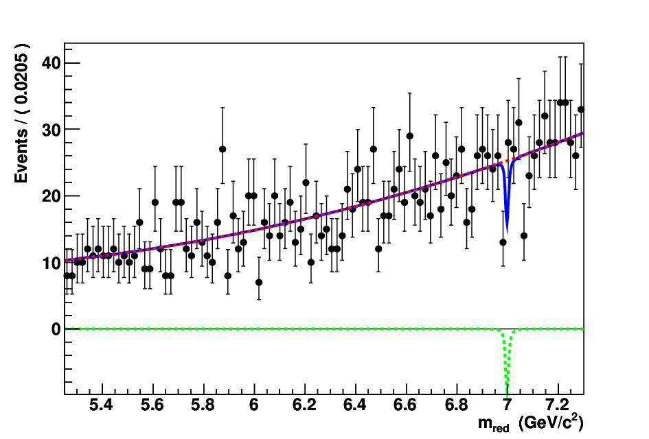


2 Fit validation using Toy Monte-Carlo
We use a large number of toy Monte-Carlo experiments to validate the fit procedure further. We first fit the background PDF’s to the cocktail samples. Then, we generate the background events according to those PDFs, setting the background yields to the number expected in the Run7 Onpeak datasets. The toy studies are done with different embedded signal events for each points.
The average fit-residuals (the difference between the number of fitted and generated events) as a function of embedded signal events for each are summarized in Appendix 9 in Figure 1 – 3 for and in Figure 4 – 6 for . The fit-residual as a function of embedded signal event is fitted by a linear function. We accumulate the intercept value of the regression in a histogram for all the known mass points for both and [Figure 10]. Since we do not observe any significant bias in the fitting procedure, we assign the RMS value of the intercept of the regression as a systematic uncertainty. The RMS value of fit bias is found to be 0.17 for and 0.22 for , which will be considered as an additional source of systematic uncertainty for and datasets.


4 Unblinding the datasets.
After finalizing all the selection criteria and the ML fitting procedure, including the validation of the analysis, we have unblinded the million events (sum of the “High” and “Medium” samples) and million events.
A total of 11,136 and 3,857 candidates are selected by the selection criteria (mentioned in section 5) in the unblinded data samples of . Figure 11 and Figure 12 show the distributions of the and together with the remaining background MC samples of , decays. The MCs are normalized to the data luminosity.


Two peaking components corresponding to and mesons are observed in the dataset. The -mesons are mainly produced in initial state radiation events, along with two or more pions, which disappears if we require both candidates to be identified as muons in the reconstruction (Figure 13) or apply a tighter () mass window cut on the distribution. An enhancement of the background is observed outside the signal region of [9.455,9.48] in the distribution of the dataset (Figure 14). This data sample is used to model the background using a sum of a Gaussian and a constant linear function (Figure 14). The fixed PDF parameters of the Gaussian function are used to describe the peak in the final fit.


To understand the peaking component at the mass position in the dataset, we compute the mass of the system recoiling against the photon, which is defined as:
| (12) |
where is the CM energy of the system and is the CM energy of the photon. The should peak at the mass position of the resonance, in an ISR decay like . Figure 16 shows the distribution in both region of as well as the outside of this region using onpeak dataset. It is clear that the distribution peaks at mass position for the region of . We have also processed a sample of with generic decays of . The distribution of generic sample at mass position is shown in Figure 17 (left). The distribution of generic sample is also shown in Figure 17 (right), which peaks at mass position. Using MC-Truth information of the survived MC events for generic decays, it is observed that about of the events decay via and about of the events decay via channel (Figure 18). We model the peaking component of the J/ background by a CB function using data sample of this generic decays (Figure 19). A high statistics data and MC samples of , , have also been used to check the resolution of distribution at the mass peak position. We find a resolution of in the data, compatible with the predictions of the MC of GeV/, which is obtained by applying the mass constraints on the to improve the resolution of the . A similar exercise without the mass constraint results in a agreement between data and Monte Carlo as well. However, the resolution of these event is not representative of that of the signal, because the kinematic is different.


5 Signal yield extraction using the 1d ML fit
We perform the likelihood scan for any possible peaks in the distribution using the unblinded onpeak data-set in the steps of half of resolution, corresponding to 4585 points. The mass region in the dataset, defined as , is excluded from the search due to large background from decays. The projection plots for selected mass points are shown in Figure 20 and 21. Figure 22 shows the number of signal events as well as signal significance for the ; ; decay as a function of . Figure 23 shows the distribution of signal significance (), where is excluded in the range of . The significance is expected to follow a normal distribution with and for the pure background hypothesis. The largest values of significance are found to be 3.62 (2.96) in the () dataset, and 3.24 for the combined dataset.


(a) (b)


(c) (d)


(e) (f)


(a) (b)


(c) (d)


(e) (f)


6 Trial factor study: true significance observation
When we search for a narrow resonance for at unknown mass points over a broad range of background, special care must be exercised in evaluating the true significance of observing a local excess of events. The log-likelihood ratio method is used to compute the significance of any positive signal observation. Since we need to scan the distribution of the onpeaks datasets at 4585 points, we should expect at least a few statistical fluctuations at the level of , even for the null hypothesis. Hence, we need to determine the probability for the background fluctuation to a particular value of anywhere in a given range.
We generate toy Monte-Calro data according to the PDFs using the background only hypothesis. We then scan the toy data in the same way as was done for the onpeak data-sets for all 4585 points, and pick up one of the maximum value of significance from these 4585 points. We repeat this process about times and accumulate the value each time in a histogram. We also compute the for the combined datasets.
We compute the inverse cumulative distribution (also called p-value) of while integrating the PDF of from to . The histograms of and its inverse cumulative distribution for , and combined datasets are shown in Figure 24, 25 and 26, respectively. The p-value is the probability of a test statistics that describes the chance that a pure background would fluctuate to a signal peak with the significance . If the null hypothesis is correct, the p-value is uniformly distributed between zero and one. To express a given value of probability in terms of standard deviations (), a convention is adopted for one sided Gaussian value of for and for .


We estimate the probability to observe a fluctuation of () in the () data-set to be (), and in the combined data-set to be based upon this trial factor study. Hence we interpret the observed local excess of events at several mass points in both the datasets as a mere background fluctuations.
7 Chapter Summary
In this chapter we have described the ML fit procedures used to extract the signal yield from the data. We have developed the signal and background PDFs using the signal MC samples generated at 26 points and the combined background MC. The fit validations are performed using a cocktail sample as well as a large number of Toy MC experiments with different embedded signal events at selected points. The signal yields are extracted using the unblinded data of . A trial factor study is also performed, which shows that there is no evidence for the di-muon decay of the in the radiative decays of the in the data samples. The next chapter will describe the possible sources of systematic uncertainties for this analysis.
Chapter 5 Systematic Uncertainties
This chapter describes the sources of the systematic uncertainty which we consider in this analysis. Two kinds of systematic uncertainties are identified, which are additive and multiplicative systematics. The additive systematics reduce the significance of any observed peak and does not scale with the number of reconstructed events. It arises from the uncertainty on the PDF parameters and the fit bias. The multiplicative systematics do not change the significance of any observed peak and scales with the number of reconstructed events. The primary contributions to the multiplicative systematic uncertainties come from the RF classifier selection, muon-ID, photon-selection, tracking and kinematic fit .
1 PDF systematics
The dominant contribution to the additive systematic uncertainty comes from the uncertainties in the extracted signal yield (), which are primarily due to uncertainties in the PDF shapes. We evaluate the PDF systematic uncertainties after unblinding the Run7 onpeak datasets by varying each parameter by its statistical error and observing the change in the fitted signal yield . The total systematic uncertainty in the signal yield is given by , where and C is the parameter correlation matrix, giving a systematic uncertainty in the signal yield. The value is found to be very small for most of the points and it varies from (0.00 – 0.62) events for the dataset and (0.04 – 0.58) events for dataset.
2 Fit Bias
We perform a study of fit bias on the signal yield with a large number of Toy MC experiments as mentioned in section 2. The biases are consistent with zero and their average uncertainty is taken as a systematic uncertainty.
3 Systematic uncertainty for Particle ID
The systematic uncertainty for muon PID selection cuts is evaluated by a standard PID weighting recipe developed by the PID group in BABAR experiment [90]. This recipe creates a map that assigns a weight of each selected track, where weight is the ratio of efficiency in data and MC. Weight comes from the PID tables, which include the central value of weight, statistical uncertainty of weight, and status of given charged tracks. We first apply all the optimal selection cuts (excluding muon ID cut) to the signal MC sample in the mass range of 0.212 – 9.46 GeV/. Then we check the status of charged tracks after applying the OR-muon PID (BDTMuon1IDFakeRate BDTMuon2IDFakeRate) selection cut. Figure 1 shows PID-weight status distribution for muon PID selection cut for both and .


We construct a new table by generating 10000 Gaussian random number with mean = PIDweight, and sigma = PIDweighterr for the PIDWeightstatus = 1, 2 and 3, where 1 means the PID efficiency of data and MC are well measured, 2 means the PID efficiency in data and MC are poorly measured due to limited statistics, but still ok, and 3 means the PID efficiency in MC is zero, but upper limit in the weight is compatible with that of a lower momentum bin, from which the PIDweight and PIDweighterr have been taken. For other PIDWeightstatus, we have used Gaussian mean = 1 and sigma = 0. Figure 2 shows the new generated PIDweight distribution (mean value of each Gaussian random number) for OR-muon PID selection cut for both and . The systematic uncertainty on the muon PID efficiency is taken as the RMS value of the Gaussian. We find that the systematic uncertainty on the muon PID is () for ().


4 Systematic uncertainty for the charged tracks
The systematic uncertainties for the four charged tracks are taken from [91], which results in a systematic uncertainty of for the two highly energetic muon tracks. The systematic uncertainty for the pions with MeV/c is taken from the soft-pion study and for tracks with GeV/c, the systematic uncertainty is taken from the Tau31 study as discussed in [91]. Figure 3 shows that around (20.6) () signal MC events lie in the range of MeV/c (for both pions) and (79.4) signal MC events lie in the range of MeV/c for () dataset. So we evaluate the uncertainty due to the reconstruction of both pions to be 1.99 () and the total systematic uncertainty for the four tracks to be () for ().


(a) (b)


(a) (b)
5 Systematic uncertainty for kinematic fit
We use the test sample of generic MC and the onpeak data samples to evaluate the systematic uncertainties for kinematic fit after unblinding the data samples. We first apply all the optimal selection cuts to the generic MC and the onpeak data samples except kinematic fit cut. We then apply kinematic fit to the both data and MC to calculate the systematic uncertainties. Figure 4 shows the kinematic fit distributions for both and . The relative number of events for both data and MC after applying the kinematic fit cut for both and are summarized in Table1. The systematic uncertainty due to the kinematic fit are found to be 1.52 and 2.96 for the and , respectively.


| Selection cuts | Data | MC | Data | MC |
|---|---|---|---|---|
| Pre-selection cuts | 13264 | 7508 | 4706 | 2682 |
| 300 | 11136 | 6402 | 3857 | 2267 |
| Efficiency | ||||
6 Systematic uncertainty for
The uncertainties on the branching fractions are and for and datasets, respectively, which are taken from the PDG [92]
7 Systematic uncertainty for RF-selection
We study the systematic uncertainties for pion related variables using a control data and MC samples of as mentioned in section 4. Figure 5 shows the data and MC comparison of the output of RF for both and datasets and the relative number of events for both data and MC after applying RF cut are summarized in Table 2. Based on the relative difference in the efficiencies of the RF cut on the data and MC, we assign a systematic uncertainty of for the dataset and for the dataset.


| Selection cuts | Data | MC | Data | MC |
|---|---|---|---|---|
| Pre-selection cut | 189644 | 1655701 | 66147 | 169913 |
| RF 0.388 (0.568) for () | 183663 | 1642292 | 60116 | 157834 |
| Efficiency | ||||
8 Systematic uncertainty due to photon selection
The systematic uncertainty related to the photon selection is measured using an sample in which one of the photon converts into an pair in the detector material [57]. The relative selection efficiencies of the photon selection variables are summarized in Table 3 and we assign a systematic uncertainty of for the photon related variables in the dataset. Since the photon selection criteria are similar in both and datasets, we use the same systematic uncertainty value for .
| For dataset | ||
|---|---|---|
| Selection cuts | Efficiency (Data) | Efficiency (MC) |
| e2Mag 0.2 | ||
| Lateral moment [0.06, 0.74] | ||
| Zernika-42 moment 0.1 | ||
| Total Efficiency | ||
9 Systematic uncertainty for counting
The systematic uncertainty for counting has been studied using the on-resonance and off-resonance samples of data, and the MC samples [93]. The number of events passing a set of selection criteria in an on-resonance sample is equal to the total number of hadronic events selected less the number of non- events. The number of non- events can be expressed in terms of the production cross section, the efficiency to pass the cuts, and the luminosity. The off-resonance sample is used to separate the number of non- events. A sample of events is also used to provide a relative luminosity normalization between between resonant and non-resonant samples. This study quotes a systematic uncertainty of . We also use this systematic uncertainty value for .
1 Final systematic uncertainties
Table 4 summarizes the final systematic uncertainties and their sources for both and , which will be incorporated to evaluate the branching ratio or upper limit of B.R. in the analysis.
| Uncertainty | ||
| Source | ||
| Additive systematic uncertainties (events) | ||
| (0.00 – 0.62) | (0.04 – 0.58) | |
| Fit Bias | 0.22 | 0.17 |
| Total | (0.22 – 0.66) | (0.18 – 0.60) |
| Multiplicative systematic uncertainties () | ||
| Muon-ID | 4.30 | 4.25 |
| Charged tracks | 3.73 | 3.50 |
| kinematic fit | 1.52 | 2.96 |
| 2.20 | 2.30 | |
| RF selection | 2.21 | 2.16 |
| Photon efficiency | 1.96 | 1.96 |
| 0.86 | 0.86 | |
| Total | 7.00 | 7.32 |
10 Chapter Summary
In this chapter, we have summarized the possible sources of the systematic uncertainties for this analysis. These systematic uncertainties are included by convolving the likelihood curve with a Gaussian of width , which is used to compute the confidence level (C.L.) upper limit using the Bayesian approach with an uniform prior. The details are discussed in the next chapter.
Chapter 6 Results and Conclusion
This chapter presents the C.L. Bayesian upper limits on the product branching fraction of as well as the effective Yukawa coupling of the b-quark to the as a function of , which are calculated in the absence of any signal events. Finally, we present the summary and conclusion of this dissertation.
1 Upper-limit
As discussed in section 6, the trial factor study shows that we find no evidence of signal for the di-muon decay of a light -odd scalar particle in the radiative decays in the samples. In the absence of any significant signal yield, we calculate the C.L upper limit on the product branching fraction as a function of , including the systematic uncertainties. The systematic uncertainty is included by convolving the likelihood curve with a Gaussian of width . A convolution is an integral that blends one function with another producing new function that is typically viewed as modified version of the original functions. Mathematically, the convolution of the two functions and over an infinite range is given by:
| (1) |
where is the modified version of original functions and after the convolution. We plot the negative log likelihood (NLL) as a function of branching fraction () and integrate it from zero upward until we find an integral which yields of the total integral (above zero) under the likelihood curve to compute the confidence level Bayesian upper limits. The is defined as:
| (2) |
where is the number of the fitted signal yield, is the signal selection efficiency, is the branching fraction of transitions, and is the number of mesons used in this analysis. For combining the results of the datasets, we add the log of the likelihoods. Figure 1 shows the likelihood function as a function of at selected mass points for , and combined data of . The correlated and uncorrelated systematic uncertainties are taken into account for combining the two datasets. The systematic uncertainties of counting, photon efficiency, tracking and PID are considered as correlated systematic uncertainties and rest of the systematic uncertainties discussed Table 4 are considered as uncorrelated systematic uncertainties. The mass region in the dataset, defined as , is excluded from the search due to a large background from . Figure 2 shows the C.L upper limits on as a function of . The limits vary between for the dataset, for the dataset, and for the combined dataset.


The branching fractions of are related to the effective Yukawa coupling () of the -quark to the via Equation 23. The value of incorporates the dependent QCD and relativistic corrections to [48], as well as the leptonic width of [50]. These corrections are as large as to first order in strong coupling constant (), but have comparable uncertainties [94]. The 90 C.L. upper limits on for combined datasets range from to depending upon the mass of , which is shown in Figure 4(a). For comparison, the results from previous BABAR measurements of , [54] are also shown. We combine our results with previous BABAR measurements [54], taking into account both correlated and uncorrelated uncertainties. Figure 3 shows the likelihood function as a function of at selected points for the combined data of , previous BABAR measurements [54] and combination of these two measurements. The combined upper limits on for these two measurements vary in the range of for (Figure 4(b)).


2 Summary and Conclusion
This thesis describes a search for di-muon decays of a low-mass Higgs boson in the fully reconstructed decay chain of , , . The sample is selected by tagging the pion pair in the transitions, using a data sample of and mesons collected with the BABAR detector at the PEP-II asymmetric-energy collider located at SLAC National Accelerator Laboratory. The is assumed to be a scalar or pseudoscalar particle with a negligible decay width compared to the experimental resolution [30]. We find no evidence for production and set confidence level (C.L.) upper limits on the product branching fraction in the range of for . These results improve the current best limits by a factor of 2–3 for and are comparable to the previous BABAR result [54] in the mass range of . Within this range, our limits rule out substantial amount of the parameter space allowed by the light Higgs [41] and axion [43] model. We also combine our results with previous BABAR results of , to set limits on the effective coupling () of the -quarks to the , , at the level of for . The combined limits on the product are the most stringent to date, and significantly constrain the theoretical Models. A high luminosity asymmetric energy Super-B factory and International Linear Collider (ILC) experiments can significantly improve the searches of these low-mass scalar particles, difficult to explore by the LHC, and elucidate the structure of the new Physics.
Chapter 7 Signal PDFs
Appendix 7.A Signal PDFs for


(a) (b) (c)


(d) (e) (f)


(g) (h) (i)


(a) (b) (c)


(d) (e) (f)


(g) (h) (i)


(a) (b) (c)


(d) (e) (f)
Appendix 7.B Signal PDFs for


(a) (b) (c)


(d) (e) (f)


(g) (h) (i)


(a) (b) (c)


(d) (e) (f)


(g) (h) (i)


(a) (b) (c)


(d) (e) (f)
Chapter 8 Background PDFs
Appendix 8.A Background PDFs for


(a) (b) (c)


(d) (e) (f)


(g) (h) (i)
Appendix 8.B Background PDFs for


(a) (b) (c)


(d) (e) (f)


(g) (h)
Chapter 9 Toy Monte Carlo Results
Appendix 9.A For


(a) (b) (c)


(d) (e) (f)


(g) (h)


Appendix 9.B For


(a) (b) (c)


(d) (e) (f)


(g) (h)


References
- [1] S. Weinberg, Phys. Rev. Lett. 19, 1264 (1967); A. Salam, in Elementary Particle Theory, edited by N. Svartholm (Almquist and Wiksells, Stockholm, 1969), p. 367; S. L. Glashow, Nucl. Phys. 22, 579 (1961); S. L. Glashow, J. Iliopoulos, and L. Maiani, Phys. Rev. D 2, 1285 (1970).
- [2] G. ’t Hooft and M. Veltman, Nucl. Phys. B44, 189 (1972).
- [3] M. J. Herrero, arXiv:hep-ph/9812242 (1998).
- [4] ‘Quarks and Leptons’: An introductory course in Modern Particle Physics, F. Halzen and A. D. Martin, John Wiley Sons, UK (1984); Introduction to Elementary Particle Physics, A. Bettini, Cambridge University Press, UK (2008); Introduction to Elementary Particle, D. Griffiths, John Wiley Sons, InC (2004).
- [5] S. Dawson, arXiv:hep-ph/9901280 (1999).
- [6] P. W. Higgs, Phys. Lett. 12, 132 (1964); P. W. Higgs, Phys. Rev. Lett. 13, 508 (1964); P. W. Higgs, Phys. Rev. 145, 1156 (1966).
- [7] F. Englert and R. Brout, Phys. Rev. Lett. 13, 321 (1964).
- [8] G. S. Guralnik, C. R. Hagen and T. W. B. Kibble, Phys. Rev. Lett. 13, 585 (1964).
- [9] T. W. B. Kibble, Phys. Rev. 155, 1554 (1967).
- [10] G. Aad, et al. [Atlas Collaboration], Phys. Lett. B716, 1–29 (2012); S. Chatrchyan, et al. [CMS Collaboration], Phys. Lett. B716, 30–61 (2012).
- [11] R. P. FeynMan, Phys. Rev. 76, 769–789 (1949).
- [12] ‘QCD and collider physics’, R.K. Ellis, W. J. Stirling and B. R. Webber, Cambridge University Press (1996); ‘Foundation of Quantum Chromodynamic’, T. Muta, World Scientific, Singapur (1987); ‘The Theory of Quarks and Gluon Interaction’, F. J. Yndurain, Springer-Verlag 2nd. Edition (1993).
- [13] S.L Glashow, Nucl. Phys. 22, 579 (1961).
- [14] L. Pape and D. Treille, Rep. Prog. Phys. 69, 2843–3067 (2006).
- [15] S.P. Martin, arXiv:hep-ph/9709356 (2011).
- [16] H. Georgi and S.L. Glashow, Phy. Rev. Lett. 32, 438 (1974).
- [17] J. C. Pati and A. Salam, Phys. Rev. D 10, 275 (1974).
- [18] H. Georgi, H.R. Quinn, and S. Weinberg, Phys. Rev. Lett. 33 451 (1974).
- [19] V. Trimble, Ann. Rev.of Astro and Astrophys. 25, 425–472 (1987).
- [20] L. Bergstrom, Rept. Prog. Phys. 63, 793 (2000).
- [21] R. W. Schnee, AIPConf. Proc. 903, 8–15 (2007; arXiv:astro-ph/0612565 (2007).
- [22] D. I. Kazakov, arXiv:hep-ph/0012288 (2001).
- [23] I. J. R. Aitchison, arXiv:0505105 (2005); H. E. Haber and G. L. Kane, Phys. Rep. 117, 75 (1985).
- [24] U. Ellwanger, C. Hugonie and A.M. Teixeira, Phys. Reports 496 1-77 (2010); J. Ellis, J. F. Gunion, H.E. Haber, L. Roszkowski and F. Zwirner, Phys. Rev. D 39 844 (1989).
- [25] R. Dermisek and J.F. Gunion, Phys. Rev. Lett. 95, 041801 (2005);
- [26] G. Hiller, Phys. Rev. D 70, 034018 (2004)
- [27] J. E. Kim and H. P. Niles, Phys. Lett. B 138 (1984) 150.
- [28] R. D. Peccei and H. R. Quinn, Phys. Rev. Lett. 38, 1440 (1977).
- [29] B. A. Dobrescu, G. Landsberg and K. T. Matchev, Phys. Rev. D 63, 075003 (2001); B. A. Dobrescu and K. T. Matchev, J. High Energy Phys. 09, 031 (2000).
- [30] E. Fullana and M.A. Sanchis-Lozano, Phys. Lett. B 653, 67 (2007).
- [31] F. Domingo, U. Ellwanger, E. Fullana, C. Hugonie and M.A. Sanchis-Lazano, JHEP 0901, 061 (2009).
- [32] S. Schael et al. [ALEPH collaboration], Eur. Phys. J. C 47, 547 (2006).
- [33] R. Dermisek and J.F. Gunion, Phys. Rev. D 73, 111701 (2006).
- [34] R. Dermisek and J.F. Gunion, Phys. Rev. D 77, 015013 (2008).
- [35] R. Dermisek and J.F. Gunion, Phys. Rev. D 75, 075019 (2007).
- [36] S. Moretti, S. Munir and P. Poulose, Phys. Lett. B 644, 241 (2007); S. Chang, P. J. Fox and N. Weiner, Phys. Rev. Lett. 98 111802 (2007); T. Stelzer, S. Wiesenfeldt and S. Willenbrock, Phys. Rev. D 75, 077701 (2007).
- [37] R. Dermisek and J.F. Gunion, Phys. Rev. D 76, 095006 (2007).
- [38] M. Drees and K. Hikasa, Phys. Rev. D 41, 1547 (2007).
- [39] M. A. Sanchis-Lazano, Mod. Phys. Lett. A 17, 2265 (2002); M. A. Sanchis-Lazano, Mod. Phys. Lett. A 19, 2183 (2002); M. A. Sanchis-Lazano, arXiv:hep-ph/0510374 (2006).
- [40] B. McElrath, Phys. Rev. D 72 103508 (2005).
- [41] R. Dermisek, J. F. Gunion and B. McElrath, Phys. Rev. D 76, 051105 (2007).
- [42] R. N. Hodgkinson, Phys. Lett. B 665, 219 (2008).
- [43] Y. Nomura and J. Thaler, Phys. Rev. D 79 075008 (2009).
- [44] B. Batell, M. Pospelov and A. Ritz, Phys. Rev. D 79, 115008 (2009).
- [45] J. P. Lees et al. [BABAR Collaboration], Phys. Rev. Lett. 108, 211801 (2012).
- [46] F. Wilzek, Phys. Rev. Lett. 39, 1304 (1977).
- [47] M. L. Mangano and P. Nason, Mod. Phys. Lett. A 22, 1373 (2007).
- [48] P. Nason, Phys. Lett. B 175, 223 (1986).
- [49] H. Kim, Y. Kolomensky and E. Petigura, et. al., BABAR Analysis Document 2107.
- [50] R. Barbieri et al., Phys. Lett. B 57, 455 (1975).
- [51] P. del Amo Sanchez et al. [BABAR Collaboration], Phys. Rev. Lett. 104, 191801 (2011).
- [52] J. F. Gunion, arXiv:0808.2509 (2008).
- [53] R. Dermisek and J.F. Gunion, Phys. Rev. D 81, 075003 (2010).
- [54] B. Aubert et al. [BABAR Collaboration], Phys. Rev. Lett. 103, 081803 (2009).
- [55] B. Aubert et al. [BABAR Collaboration], Phys. Rev. Lett. 103, 181801 (2009).
- [56] B. Aubert et al. [BABAR Collaboration], arXiv:0808.0017 (2008).
- [57] P. del Amo Sanchez et al. [BABAR Collaboration], Phys. Rev. Lett. 107, 021804 (2011).
- [58] J. P. Lees et al. [BABAR Collaboration], Phys. Rev. Lett. 107, 221803 (2011).
- [59] W. Love et al. [CLEO Collaboration], Phys. Rev. Lett. 101, 151802 (2008).
- [60] M. Ablikim et al. [BESIII collaboration], arXiv:1111.2112 (2011).
- [61] S. Chatrchyan et al. [CMS collaboration], Phys. Rev. Lett. 109, 121801 (2012).
- [62] F. Domingo, JHEP 1104, 016 (2011).
- [63] N. Cabibbo, Phys. Rev. Lett. 10, 531 (1963); M. Kobayashi and T. Maskawa, Prog. Theor. Phys. 49, 652 (1973).
- [64] W. Kozanecki, Nucl. Instrum. Meth., A 446, 59–64 (2000).
- [65] B. Aubert et al. [BABAR Collaboration], Nucl. Instrum. Meth., A 479, 1–116, (2002).
- [66] V. Re et al. [BABAR Collaboration], Nucl. Instrum. Meth., A 511, 1–5, (2003).
- [67] G. Benelli et al. [BABAR Collaboration], IEEE, 2, 1145–1148 (2005); W. Menges et al. [BABAR Collaboration], IEEE, 3, 1470–1474 (2005).
- [68] M. R. Convery et al. [BABAR Collaboration], Nucl. Instrum. Meth., A 556, 134–139, (2006).
- [69] R. Bartoldus et. al., BABAR Analysis Document 194.
- [70] P. F. Harison, J. Phys. G 28, 2679 (2002); A. Roodman, arXiv:physics/0312102 (2002).
- [71] D. J. Lange, Nucl. Instrum. Meth. A 462, 152 (2001).
- [72] S. Jadach, W. Placzek, B. F. L. Ward, Phys. Lett. B 390 (1997) 298.
- [73] B. F. L. Ward, S. Jadach and Z. Was, Nucl. Phys. Proc. Suppl. 116, 73 (2003).
- [74] D. Cronin-Hennessy et al. [CLEO Collaboration], Phys. Rev. D 76 072001 (2007).
- [75] S. Agostinelli et al. [GEANT4 Collaboration], Nucl. Instrum. Methods Phys. Res., Sect. A 506 250 (2003).
- [76] http://root.cern.ch/drupal/.
- [77] A. Drescher et al. [ARGUS collaboration], Nucl. Instum. Meth 237, 464 (1985).
- [78] R. Sinkus and T. Voss, Nucl. Instrum. Meth. A 391, 360 (1997).
- [79] I. Narsky, arxiv:physics/0507143v1 (2005)
- [80] J. Friedman and N. Fisher, Statistics and Computing 9, 123-143 (1999).
- [81] G. Punzi, arxiv:physics/0308063v2 (2003).
- [82] http://www.stat.berkeley.edu/ breiman/RandomForests/.
- [83] V. Prasad, B. Bhuyan and P. Poulose, BABAR Analysis Document 2304; J.P. Lees [BABAR collaboration], Phys. Rev. D 87, 031102 (R) (2013), [arXiv:1210.0287].
- [84] M. J. Oreglia, Ph.D Thesis, report SLAC-236 (1980); J.E. Gaiser, Ph.D Thesis, report SLAC-255 (1982); T. Skwarnicki, Ph.D Thesis, report DESY F31-86-02 (1986).
- [85] R. Barlow, Nucl. Instrum. Methods Phys. Res., Sect. A 297 496–506 (1990).
- [86] L. Lyons, W. W. M. Allison and P. Comellas, Nucl. Instrum. Methods Phys. Res., Sect. A 297 496–506 (1990).
- [87] http://roofit.sourceforge.net/
- [88] http://rarfit.sourceforge.net/
- [89] B. Aubert et al. [BABAR Collaboration], Phys. Rev. Lett. 88, 241801 (2002).
- [90] http://www.slac.stanford.edu/BFROOT/www/Physics/Tools/Pid/PidOnMc/nutshell.htmlweight
- [91] T. Allmendinger et al., arXiv:1207.2849.
- [92] J. Beringer et al. [Particle Data Group], Phys. Rev. D 86, 010001 (2012).
- [93] Grant MCGregor and Chris Hearty, BABAR Analysis Document 2069.
- [94] M. Beneke, A. Signer and V.A. Smirnov, Phys. Rev. Lett. 80, 2535 (1998).