H Absorption in Transiting Exoplanet Atmospheres
Abstract
Absorption of stellar H by the upper atmosphere of the planet HD189733b has recently been detected by Jensen et al. Motivated by this observation, we have developed a model for atomic hydrogen in the state and compared the resulting H line profile to the observations. The model atmosphere is in hydrostatic balance, as well as thermal and photoionization equilibrium. Collisional and radiative transitions are included in the determination of the state level population. We find that H absorption is dominated by an optical depth shell, composed of hydrogen in the metastable 2s state that is located below the hydrogen ionization layer. The number density of the 2s state within the shell is found to vary slowly with radius, while that of the 1s state falls rapidly. Thus while the Ly absorption, for a certain wavelength, occurs inside a relatively well defined impact parameter, the contribution to H absorption is roughly uniform over the entire atomic hydrogen layer. The model can approximately reproduce the observed Ly and H integrated transit depths for HD189733b by using an ionization rate enhanced over that expected for the star by an order of magnitude. For HD 209458b, we are unable to explain the asymmetric H line profile observed by Jensen et al., as the model produces a symmetric line profile with transit depth comparable to that of HD 189733b. In an appendix, we study the effect of the stellar Ly absorption on the net cooling rate.
Subject headings
line: formation – planets and satellites: atmospheres – stars: individual (HD 189733, HD 209458)I. Introduction
Absorption11 1 We will use the term “absorption” thoughout the paper, even though at the low densities of interest each radiative transition is likely followed by a (resonant scattering) or (resonance fluorescence) radiative transition. Either outcome will prevent the stellar H photon from reaching the observer. of starlight by a transiting planet provides a probe of the atmospheric composition and structure. The Ly and H transitions of hydrogen may potentially give rise to large transit depths, as the combination of large cross section and hydrogen abundance put the optical depth unity surfaces at much higher altitudes ( pressure levels) than the continuum photosphere (mbar - bar).
The detection of Ly absorption [25, 27, 26, 2, 3, 7, 17, 8, 18] due to atoms in the ground state traces the bulk of the atomic population, and hence the density profile of the planet’s atmosphere. By contrast, the recent detection of H absorption by Jensen et al. [13] reveals the small population in the excited state. As the number density in the state depends sensitively on the excitation rates due to collisions and radiative pumping by the stellar photons, it is a much more sensitive probe of the atmosphere, in particular the temperature profile. Hence, the Ly and H lines are complementary probes of the atomic hydrogen layer.
The goal of this paper is to construct a detailed model of the state population by which to understand the Jensen et al. [13] H transit depth of HD 189733b. Section II reviews the relevant observations of Ly and H observations for HD 209458b and HD 189733b. Section III presents the details of the atmospheric model. Section IV presents numerical results for HD 189733b, and a detailed comparison to the Jensen et al. [13] data. Section V presents the predictions of our model for HD 209458b, and they disagree significantly with the data. Section VI addresses the possibility of observing Balmer continuum absorption. We summarize our results and compare to previous investigations in Section VII. In the appendix, we study the effect of the stellar Ly on the cooling rate.
II. Review of the Observations
We first review the observations of H absorption that motivate our work, as well as previous attempts to determine excited state abundance, or excitation temperature, from the observations. These previous estimates of density and temperature will be compared to the calculations in this paper in Section VII.
The initial detection of Ly absorption during the transit of HD209458b [25] indicated a decrease in flux over a wavelength band around line center. The implied occultation radius of , where is the radius of Jupiter, is larger than the Roche lobe radius of , leading the authors to suggest that the planet must be in a state of Roche lobe overflow. Due to absorption by the interstellar medium and geocoronal emission, the center of the Ly line cannot be used, and absorption is only reliably observed outside from line center, indicating either a population of “hot hydrogen” () formed through charge exchange with stellar wind protons [11, 9, 24] or large columns of “warm hydrogen” (; Yelle 30), which yield a saturated line. This paper attempts to explain H transit spectra by the latter scenario of a large column of warm hydrogen.
For , the observed Ly absorption is well out on the damping wing of the line, and hence the cross section is not a strong function of temperature. The Ly transit depth is, however, dependent on the temperature through the atmospheric scale height. As we will show, the H absorption is expected to have a stronger dependence on temperature due to the collisional excitation rate of the to transition.
| Mass () | 1.138 |
|---|---|
| Radius () | 1.138 |
| a (AU) | 0.031 |
The first attempt to detect H was by Winn et al. [28] who observed HD209458. For the remainder of this section, we summarize their observational results, assumptions, and inferences. Integrating over a band, they find an equivalent width
| (1) |
where and are the flux in and out of transit, respectively. If the state hydrogen occults an area , and the area of the star is , then in the optically thin limit, eq. (1) can be used to relate the column density of the state, , to the equivalent width as 22 2 We believe eq.6 of Winn et al. [28] and eq.4 in Jensen et al. [13] should have on the right hand side, not the left, as the drop in observed flux is proportional to the occulting area, not its inverse. Their estimates of should be multiplied by the factor , implying columns larger by a factor .
| (2) |
Here is the wavelength of the transition, and is the oscillator strength. Using a fractional area from Ly measurements [25], and assuming the same occulting area for Ly and H lines, the column density can be constrained to be .
H absorption was subsequently detected by Jensen et al. [13] in the transits of HD 209458b and HD 189733b. The line profile of HD 209458b showed an excess to the blue and a deficit to the red of line center, for which we have no simple explanation. The line profile of HD 189733b offered no such consternation, exhibiting a symmetric absorption feature about line center. HD 189733b is the focus of our modeling effort.
To quantify the absorption, Jensen et al. [13] introduce the absorption measure , defined as
| (3) |
where
| (4) |
and i=blue, red, central indicates the domain of the wavelength integration. The purpose of subtracting off the bands just outside the line center is to derive the drop in flux due to the upper atmosphere, where the H absorption takes place; absorption of the neighboring continuum takes place much deeper in the planet’s atmosphere, near the continuum photospheres at mbar-bar pressures. In their analysis, Jensen et al. [13] considered three bands with the central band covering the H line and blue and red being adjacent bands at shorter and longer wavelengths, respectively. The absorption measure can be related back to equivalent width by . For HD 189733b, the absorption measure is [13].
Winn et al. [28] and Jensen et al. [13] estimate the excitation temperature, , starting with the Boltzmann distribution for the number densities and of atoms in states and :
| (5) |
where and are the degeneracies of each state, including both 2s and 2p upper states, and the energy difference is eV. The authors then estimate the left hand side by equating , where is the column density of ground state hydrogen. This assumption relies on the distribution of and being similar in the atmosphere, so that the effective path length in the integration is comparable. Lastly, they assume that , which is valid if both transitions are optically thin and the occulting area is the same for each. Plugging this into the left hand side and solving then gives . This high excitation temperature is not achieved for thermal gas in any published models to date (e.g. Yelle 30, Murray-Clay et al. 19, García Muñoz 10). We will revisit the estimates of in section VII in the context of our model for the atmospheric structure and level populations.
III. Model for the Atmosphere
In this section we present our model for the density and temperature profiles and the hydrogen level populations. Section III.1 outlines the different layers of the atmosphere of interest. Section III.2 discusses thermal and ionization equilibrium. Section III.3 presents the rate-equilibrium equations which determine the ground and excited state populations of hydrogen. Section III.4 discusses the numerical solution of the coupled equations of hydrostatic balance, thermal equilibrium photoionization equilibrium and detailed balance for the level populations.
III.1. Basic Structure of the Atmosphere

We consider a spherically symmetric atmosphere above the photospheric radius at , where is the spherical radius. The atmosphere is divided into three zones (see Figure 1), according to the state of hydrogen: molecular, atomic and ionized. Inside the photospheric radius, , we consider the planet to be opaque to H. The shell is composed mainly of molecular gas, due to the low temperature. Assuming a Boltzmann distribution and a mean temperature of , the equilibrium temperature (for zero albedo) of HD189733b, the relative abundance of hydrogen is , where and are the number density of hydrogen in the and states, respectively (we use for both number density and radial quantum number. The meaning is clear from the context). Due to the small abundances and low temperatures, we assume that the contribution of the molecular layer to the H absorption is negligible. The transition from molecular to atomic hydrogen takes place at a radius , and it is this “atomic” layer at and that gives rise to the H absorption in our model. At pressures hydrogen will be mostly photoionized, forming an “ionized” layer that contributes little to the H absorption.
A parameter that enters our model is the base radius of the atomic layer . It is determined by the photospheric radius and the thickness of the molecular layer . If the molecular layer is isothermal at temperature , the thickness is
| (6) |
where is the mean molecular weight, is the mass of the planet, is the pressure of the optical photosphere, and is the pressure at the molecular-to-atomic transition. For , and , the thickness is . An upper bound to the thickness is found using the dissociation temperature at which the gas transitions from molecular to atomic. Plugging into the Saha equation, and using the roto-vibrational energies from Borysow et al. [4], we find and . Since the equilibrium and dissociation temperature estimates differ by only 40%, and both give altitudes which are a small fraction of , we conclude the thickness of the molecular layer will not greatly affect the H transit depth. Henceforth we use in numerical calculations for HD 189733b.
III.2. Ionization and Thermal Equilibrium
| Number | Reaction | Symbol | Rate | Reference |
|---|---|---|---|---|
| R1 | See Eq. 9 | |||
| R2 | Draine [6] | |||
| R3 | Janev et al. [12] | |||
| R4 | Janev et al. [12] | |||
| R5 | Janev et al. [12] | |||
| R6 | See Eq. 11 | |||
| R7 | See Eq. 11 | |||
| R8 | Draine [6] | |||
| R9 | Draine [6] | |||
| R10 | Osterbrock & Ferland [20] | |||
| R11 | Osterbrock & Ferland [20] | |||
| R12 | Ly cooling |
The electron and ion abundances are set by rate equilibrium between photoionization of ground-state hydrogen and radiative recombination,
| (7) |
Here is the photoionization rate from the 1s state, defined in eq. 9 below, and is the Case B recombination coefficient defined in Table 2. As discussed below, we assume all free electrons come from hydrogen so that .
The heating rate is dominated by photoelectrons from the ionization of hydrogen. In the high-UV case we consider here, cooling will be dominated by Ly emission [19]. The temperature is then determined by balancing photoelectric heating () and Ly cooling (),
| (8) |
where the Ly cooling rate is and and are the collisional excitation rates from the 1s state to the 2s and 2p states, respectively (see table 2). Excitation to the 2s state also contributes to Ly cooling since the -mixing reactions rapidly turn 2s into 2p, which then emits a Ly photon (see Figures 12 and 13). In eq.8, is the heating rate per particle, defined in eq.10 below.
In cases where there is a non-zero Ly excitation rate due to the stellar radiation field, there exists the possibility, for sufficiently low gas temperatures, of Ly heating when the excitation temperature of the radiation field approaches or exceeds the gas temperature. In the appendix, we estimate the contribution of true Ly absorption to the overall heating rate as a function of and T. We find that for the solar value of , the cooling rate is not significantly altered by the inclusion Ly heating for the bulk of the layer that is responsible for the H absorption; however, the heating could be important at lower temperatures near the base of the atomic layer (see fig. 16). To address this issue fully it is necessary to have a detailed treatment of Ly radiation transfer which is beyond the scope of this paper.
While some parameters of the planet are well known (see table 1), such as planetary mass (), radius () and semi-major axis (), other parameters are less certain, and may even vary with time, such as the ionizing and Ly flux of the star HD 189733. Also uncertain is the role of day-night transport of heat in the upper atmosphere [14]. Given these uncertainties, we parametrize the ionizing flux of HD 189733, and hence the heating and ionization rates, in an attempt to explain the observed transit depth and line profile. Specifically, the ionization rates will be multiplied by a factor . The flux averaged over steradians corresponds to . The substellar flux corresponds to . Ionization rates larger than the nominal substellar value have . For the Ly rate, we use the solar spectrum and evaluate the flux at the orbital separation of HD 189733b. We take the value of to be constant throughout the atmosphere.


The ground-state photoionization and photoelectric heating rates are defined as
| (9) |
and
| (10) |
where is the mean stellar intensity, is the 1s state column density, is the ionization threshold frequency, and is the photoionization cross sections for the 1s state [20]. The ultraviolet spectrum is a synthetic spectra for HD 189733b downloaded from the X-exoplanets Archive at the CAB [21]. The integration over frequency allows higher energy photons to dominate the integral at larger depth [23], leading to a larger rate than if a single frequency was used [19]. Figs. 2 and 3 show the photoionization and heating rates due to the 1s state as a function of , evaluated for HD189733b. At small , the optically thin limit, the rates are constant, while at large columns they decrease roughly as a power law.
Although ionization of the state hydrogen contributes negligibly to the electron density, ionization has an important effect on the number densities and of the 2s and 2p states. The rates are given by
| (11) |
where is the frequency threshold for state ionization. The upper frequency bound of is included since photoionization of the ground state will both quickly attenuate ionizing radiation above this frequency and will contribute negligibly to the photoionization rate due to the small cross-section. The spectrum used is taken from the Castelli and Kurucz Atlas [5]. We omit the factor of one quarter found in Eqn. 9 due to the fact that Balmer continuum photons are optically thin throughout the region of interest, making the photoionization rate insensitive to the specific geometry considered. Additionally, we have ignored attenuation of the radiation field due to the small column densities involved.
III.3. Level Populations
In the upper atmosphere, several different physical processes are important in setting the level populations, including collisional excitation and de-excitation, and bound-bound and bound-free transitions due to the stellar radiation field. The 2s and 2p states must be considered separately due to the lack of a fast radiative transition between 2s and the ground state33 3 The two photon transition has a rate of , which is much smaller than .. The equation expressing rate equilibrium for the 2p state is
| (12) | |||||
while that for the 2s state is
| (13) | |||||
Here denotes the collisional transition from state to state , and both the , and the -changing reaction are included. Collisional transitions induced by atomic and molecular hydrogen, and helium, are negligible. The terms and represent the effective recombination coefficients to that level, and include radiative cascade from higher levels [6]. We ignore ionization of helium, and assume the electrons contributed by other elements, such as sodium and potassium, are negligible in comparison to that from hydrogen, hence . The ’s and ’s are the Einstein coefficients for radiative transitions, and is transition rate associated with Ly radiation. The rate coefficients are listed in table 2.
Due to the negligible contribution from collisions, the 2p occupation is set by radiative excitation and de-excitation,
| (14) | |||||
For the analytic estimate of , we have included a dilution factor , for stellar radius and orbital separation , and the line intensity at the stellar surface is , where is the approximate excitation temperature for the solar Ly. The 2p density is small mainly due to the small stellar excitation temperature, and additionally because of the dilution factor. We show the profile of in figure 4 including all the physical effects in eq.12, verifying that radiative rates dominate, and that the 2p population is far smaller than 2s.
At sufficiently large , the 2s state is primarily populated by collisional excitation from the ground state while de-population is primarily due to the -mixing transition 2s2p. The 2s abundance can be estimated as
| (16) | |||||
where and is the Euler-Mascheroni constant.
| (17) | |||||
| (18) |
where we have defined . The heating rate scales with as and the photoionization rate scales as (see figs. 2 and 3 and Trammell et al. [23]). Along a radial path the column density can be approximated by , the 2s volume density scales as . The parameters and depend on the EUV spectrum, and for the synthetic HD189733 spectrum giving .44 4 For the solar spectrum Trammell et al. [23] found and . As a result, we find that is fairly constant over a large range of pressures in the atomic layer.
III.4. Numerical Method
We consider a one-dimensional hydrostatic profile, with uniform spherical irradiation55 5 Since there is minimal attenuation of and due to the small columns of hydrogen involved, the assumption of spherical irradiation is equivalent to irradiation in the slant geometry, as discussed in §III.2. from the outside. We integrate the equation of hydrostatic balance, and the definition of the column,
| (19) |
| (20) |
where the pressure is given by and the density is . is the fraction, by number, of helium per hydrogen nucleus, and although it is considered non-reactive in our model, it affects the profile through its contribution to the density and pressure. The relative helium abundance is considered to be constant throughout the atmosphere and is taken to have the solar value [20].
To generate the atmospheric profile, the pressure is integrated from the outer boundary using Eqn. 19 through a fourth-order Runge-Kutta scheme. Given the pressure, temperature and ionization state can be solved for using Eqns. 7 and 8. The column density is then updated using Eqn. 20 and the process repeated until the base radius is reached. To achieve the desired pressure at the base, the pressure at the outer boundary is varied using the secant method and new atmospheric profiles are generated until the target base pressure is reached.
Once the final profile is determined, the profiles for and can be calculated for the entire atmosphere using Eqns. 12 and 13.
With the radial temperature and the profile now calculated, the state column density in the slant geometry, , and the optical depth, , can be calculated as a function of impact parameter b,
| (21) |
| (22) |
where is the line-of-sight coordinate and is related to the radial coordinate and impact parameter by . We do not include in the integrals due to its negligible contribution to the overall abundance for HD189733b. The proportional reduction in flux, ignoring the opaque disk at , is then given by
| (23) |
Integrating eq. 23 with respect to wavelength recovers the equivalent width in eq. 1. We do not use this definition in practice, instead we choose to work with the absorption measure ,
| (24) | |||||
| (25) |
where is the optical depth of the ISM and is the unabsorbed stellar intensity. For Ly, we use a Voigt profile with a temperature of and assume an interstellar hydrogen column density [29, 17]. We assume no attenuation of H due to the interstellar medium. For a constant , eq.25 is equivalent to . In calculating for Ly, we assume that is proportional to
| (26) |
from Lecavelier Des Etangs et al. [17]. For H transits we assume that is constant with .
IV. Results
To study the effect of varied heating and ionization rates, we vary between 1 and 20. For each model atmosphere, we calculate for both H and Ly. For each , we consider heating and ionization rates as defined by eqs. 9 and 10, base radius , (see eq. 6) and base pressure .


Figure 4 shows the number density profile for the case. Throughout both the atomic and ionized layers is seen to roughly trace while follows the neutral hydrogen abundance, as expected from eq. 14. The profiles, shown in Figure 5, exhibit the same behavior. Within the atomic layer, maintains a roughly constant abundance despite varying by three orders of magnitude, although it is not explicitly constant, as can be seen in figs. 10 and 11. The 50% ionization point is seen to move inward in pressure approximately linearly in with the increase in ionization rate (see figs. 4 and 5).

The simulated transits for the abundance profiles in Figures 4 and 5 are shown in Figure 6, compared to the data for HD 189733b from Jensen et al. [13]. The model profiles have been computed using eq. 23. It is clear that underestimates the transit depth, while the higher ionization rate curve has roughly the correct width and depth. We note that there are significant oscillatory features in the measured data, which are much larger than the error bars shown in our Figure 6 and their Figure 3. These features persist in the wavelength regions outside the line. Jensen et al. [13] attribute these features to systematic errors not included in the error bars shown.
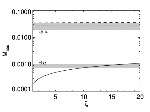
Next we vary in order to derive the best fit to the corrected width reported by Jensen et al. [13], with the corresponding values of shown in Fig. 7. Additionally, we calculate for the unresolved Ly. We find the H data are best fit by . Lecavelier Des Etangs et al. [17] determined the unresolved Ly transit depth to be , including a contribution from the photospheric disk. For the model, we find , including the opaque disk contribution, within two standard deviations of the observed value.

It is of interest to compare the location of the regions which contribute to for the H and Ly. Figure 8 shows the contribution to the integral in eq. 25 as a function of for both H and Ly. The primary contribution for Ly occurs farther out than that of H since Ly becomes optically thick throughout the integrated band at lower column densities than H. The linear decrease for decreasing is a geometric effect arising from the fact that annuli at larger impact parameters contribute more. For H, the largest contribution occurs at the base of the atomic layer with a noticeable decrease for impact parameters inside that layer. For large b, the contributions for both H and Ly are small. The constancy at large is due to the large scale height found at these radii. If a planetary wind is present, the densities at these radii could be much lower than found in our hydrostatic model (e.g., Yelle 30), further decreasing their contribution to .

Although constitutes an order-of-magnitude increase in the heating rate, the change in temperature in the atomic layer is relatively modest. If we take the volume-weighted average temperature,
| (27) |
where is the radius where the electron density equals the neutral hydrogen density (see fig. 1), . For the case, we find , and for we find . Previous investigators have found the need for additional UV heating [17]. Although we enforce this increase in temperature through an increase in the photoelectric heating rate for hydrogen, a more complete modeling of the heating and cooling processes in the atmosphere could explain the required temperature difference [15, 16].
Fig. 9 shows the temperature profiles as a function of gas pressure for both and . Within the atomic layer (), the case is approximately above the temperatures in the case at comparable pressures; however, due to the proportionately smaller ionization rate, the atomic layer extends to lower pressures for which accounts for the similar values of .
We note that the temperatures at are , much higher than the temperatures required for the formation of molecules. This is a limitation of our model due to the simplified prescriptions for heating and cooling.


The abundance profiles are shown for and in figs. 4 and 5, respectively. In both cases, traces the abundance of neutral hydrogen, as expected from eq. 14. Within the atomic layer, maintains a roughly constant abundance despite varying by three orders of magnitude. To better exhibit the small changes in , Figures 10 and 11 show a linear scale.


Fig. 12 shows the reaction rates for all reactions involved in the formation of 2s hydrogen for the model. Within the hydrogen layer, the abundance is set by the balance of collisional excitation from 1s and the -mixing reaction. As pressures decrease, and the atmosphere becomes ionized, the contribution of radiative recombination increases. Once the atmosphere becomes predominantly ionized, radiative recombination becomes the dominant formation pathway.
The reaction rates for 2p hydrogen are shown in fig. 13. Throughout the atmosphere, is set by the radiative transition between 1s and 2p, with little contribution from other rates. Attenuation of the Ly radiation could play a role in decreasing ; however, at bar pressures we find that the radiative transition rates exceed the collisional rates by a factor of .
V. The Case of HD209458b


A similar analysis has been performed for HD209458b. Since the line profiles for model and data are discrepant, we only produce a parameter study of for the same range of used above.
Using parameters taken from exoplanet.eu, we take , , , and use the simulated UV spectrum for HD209458 from the X-exoplanets Archive at the CAB [21].
Fig. 14 shows the absorption profile for . It is immediately obvious that there is no match between the model prediction and the observers profile. The model profile is symmetric about line center while and the observed profile is antisymmetric. The observed profile has a width characteristic of the orbital velocity () while the model is only a couple Doppler widths ( wide. Fig. 15 shows the dependence of on . The curve is qualitatively similar to that of the HD189733b case.
It should be noted that for HD209458b we find that 2p becomes more important than for HD189733b. Accurately accounting for 2p requires modeling the radiative transfer of the Ly which is beyond the scope of this paper.
VI. Balmer Continuum Absorption
Given the observation of Balmer continuum absorption by HD209458b [1], we estimate the transit depth for HD189733b with our model. At the Balmer edge, the bound-free absorption cross-section is with the cross section decreasing for smaller wavelengths. For , the number density is bounded and a characteristic length is . This yields an upper limit on the optical depth with smaller values of for both larger impact parameters and shorter wavelengths. The reduction in flux due to bound-free absorption relative to H absorption should be proportional to the ratio of cross sections,
| (28) | |||||
| (29) |
Within the context of our model, the transit depth due to the Balmer bound-free continuum absorption is too small to be observed for both HD189733b and HD209458b.
VII. Summary and Discussion
We have modeled the abundance of n=2 hydrogen in hydrostatic atmospheres. We find that the H absorption can be explained by metastable 2s, similar to what is found in the interstellar medium (e.g., Townes 22). The dominant mechanism for the creation of 2s hydrogen is collisional excitation from the 1s state where it subsequently collisionally transitions to the 2p state and is finally radiatively de-excited. The 2s population dominates 2p throughout the atmosphere by two orders of magnitude for the parameters used in our study, although the specifics depend on the chosen value of . We do not model the spatial variation in the intensity of Ly, instead choosing a constant value. This assumption allows us to estimate an upper limit on the 2p abundance. Since 2p remains negligible compared to 2s for our chosen , we can assume that it should similarly be negligible in the case where resonance scattering has depleted the available Ly photons. Unlike , has limited dependence on the radiation field, instead depending strongly on the gas temperature through the exponential dependence found in . We find that the data are best fit by an atomic hydrogen layer approximately hotter than our case, which corresponds to . Caution should be used in the physical interpretation of this value due to the simplified heating and cooling present in our model.
Because of the strong dependence on temperature, H should be considered a complementary probe to Ly which is relatively insensitive to the gas temperature, probing instead all the atomic gas.
This model differs from the calculations of Jensen et al. [13]. Assuming that both H and Ly are optically thin, they used eq. 2 to derive an excitation temperature of . Arguing that the levels will approach a Boltzmann distribution deeper in the atmosphere and the excitation temperatures found are not compatible with the expected gas temperature at these densities, they conclude that the absorption must occur in the planetary wind. For our model, we find which using eq. 5 gives
| (30) |
This value for is lower than the temperature in the neutral layer and is significantly lower than the value quoted by Jensen et al. [13] due to the significantly smaller abundance in our model. The former is due to the collisional excitation being balanced by the -mixing reactions, not collisional de-excitation. The latter is due to the overestimation of the gas temperature due to the assumption of optically thin Ly.
Tremblin & Chiang [24] have proposed that the H absorption can be explained by the same mechanism they use to explain Ly absorption, colliding planetary and stellar winds. This mechanism allows for Ly absorption from line center to be explained by the formation of hot () neutral hydrogen generated through charge exchange with solar wind protons. If H is in fact probing the interface between the two winds, the Ly and H lines should have comparable widths; however, the observed width for HD189733b is . Tremblin & Chiang [24] propose to explain this population of cool hydrogen in its state through cooling of the initially hot population formed through charge exchange.
We find that observed absorption of H can be explained by our model with the primary signal coming from the neutral atomic layer. Within this layer, the abundance of hydrogen is roughly constant, even though the overall abundance of hydrogen is increased by three orders of magnitude from the top of the layer to the bottom because the density increase is offset by a decrease in temperature. The transition to molecular hydrogen will lead to a downturn in the overall abundance. As a result, there should not be significant contribution to H absorption within this layer.
Although many simplifications have been made, we have included the relevant physics and reproduced the transit signal observed by Jensen et al. [13] for HD189733b. There are, however, many avenues for improving the calculation. We do not include the cooling required to cause the transition to the molecular state. This results in our model having too high a temperature at the base radius. The inclusion of the necessary physics will eliminate the need for the intermediate boundary at .
Our model also required a higher rate of heating than expected from UV models from the X-exoplanets Archive at the CAB [21]. The inclusion of heavier atomic species allows for far-UV absorption higher in the atmosphere [15, 16] which could reduce the need for the large heating rate.
Our model has assumed spherical symmetry. Due to the strong dependence of the abundances on the temperature, temperature variations between the day and night side could induce strong day-night variation in and , which will be observable since the transit probes the day-night terminator. This can partially be negated by the redistribution of thermal energy by zonal winds; however, this provides more reason to model the signal in three-dimensions, not less.
References
- [1] Ballester, G. E., Sing, D. K., & Herbert, F. 2007, Nature, 445, 511, 511
- [2] Ben-Jaffel, L. 2007, ApJ, 671, L61, L61
- [3] —. 2008, ApJ, 688, 1352, 1352
- [4] Borysow, A., Frommhold, L., & Moraldi, M. 1989, ApJ, 336, 495, 495
- [5] Castelli, F., & Kurucz, R. L. 2003, in IAU Symposium, Vol. 210, Modelling of Stellar Atmospheres, ed. N. Piskunov, W. W. Weiss, & D. F. Gray, 20P
- [6] Draine, B. T. 2011,
- [7] Ehrenreich, D., Lecavelier Des Etangs, A., Hébrard, G., et al. 2008, A&A, 483, 933, 933
- [8] Ehrenreich, D., Bourrier, V., Bonfils, X., et al. 2012, A&A, 547, A18, A18
- [9] Ekenbäck, A., Holmström, M., Wurz, P., et al. 2010, ApJ, 709, 670, 670
- [10] García Muñoz, A. 2007, Planet. Space Sci., 55, 1426, 1426
- [11] Holmström, M., Ekenbäck, A., Selsis, F., et al. 2008, Nature, 451, 970, 970
- [12] Janev, R., Reiter, D., & Samm, U. 2003, Collision Processes in Low-temperature Hydrogen Plasma, Berichte des Forschungszentrums Jülich
- [13] Jensen, A. G., Redfield, S., Endl, M., et al. 2012, ApJ, 751, 86, 86
- [14] Koskinen, T. T., Aylward, A. D., Smith, C. G. A., & Miller, S. 2007, ApJ, 661, 515, 515
- [15] Koskinen, T. T., Harris, M. J., Yelle, R. V., & Lavvas, P. 2012a, ArXiv e-prints, arXiv:1210.1536
- [16] Koskinen, T. T., Yelle, R. V., Harris, M. J., & Lavvas, P. 2012b, ArXiv e-prints, arXiv:1210.1543
- [17] Lecavelier Des Etangs, A., Ehrenreich, D., Vidal-Madjar, A., et al. 2010, A&A, 514, A72, A72
- [18] Lecavelier des Etangs, A., Bourrier, V., Wheatley, P. J., et al. 2012, A&A, 543, L4, L4
- [19] Murray-Clay, R. A., Chiang, E. I., & Murray, N. 2009, ApJ, 693, 23, 23
- [20] Osterbrock, D. E., & Ferland, G. J. 2006,
- [21] Sanz-Forcada, J., Micela, G., Ribas, I., et al. 2011, A&A, 532, A6, A6
- [22] Townes, C. H. 1957, in IAU Symposium, Vol. 4, Radio astronomy, ed. H. C. van de Hulst, 92
- [23] Trammell, G. B., Arras, P., & Li, Z.-Y. 2011, ApJ, 728, 152, 152
- [24] Tremblin, P., & Chiang, E. 2012, ArXiv e-prints, arXiv:1206.5003
- [25] Vidal-Madjar, A., Lecavelier des Etangs, A., Désert, J.-M., et al. 2003, Nature, 422, 143, 143
- [26] —. 2008, ApJ, 676, L57, L57
- [27] Vidal-Madjar, A., Désert, J.-M., Lecavelier des Etangs, A., et al. 2004, ApJ, 604, L69, L69
- [28] Winn, J. N., Suto, Y., Turner, E. L., et al. 2004, PASJ, 56, 655, 655
- [29] Wood, B. E., Redfield, S., Linsky, J. L., Müller, H.-R., & Zank, G. P. 2005, ApJS, 159, 118, 118
- [30] Yelle, R. V. 2004, Icarus, 170, 167, 167
Appendix A Net Ly Heating or Cooling Including Collisional Excitation and Thermalization of Stellar Photons
In this section we investigate the effect of the radiation field on the Ly cooling rate. The cooling rate , as used in the text, ignores the possibility of heating due to collisional de-excitation. Allowing for this possibility, the cooling rate takes the form
| (A1) |
This cooling rate depends on radiative excitation and de-excitation as well as recombination and photoionization implicitly through their effect on the level populations, and (see eqs. 12 and 13). For sufficiently low temperature or large , the collisional de-excitation rates can become comparable to the excitation rates, reducing the net cooling rate and, in extreme cases, result in net heating.
To this end, we solve eqs. 13 and 12 for and given fixed values of and . In the absence of recombination, the solution for is independent of , the dependence having been explicitly factored out in eq. A1. Even if recombination is included, it can safely be ignored so long as its contribution to the and abundance remains small. For the 2s state, where collisional excitation is the dominant formation pathway, this results in the condition
| (A2) |
For the 2p state, radiative excitation sets the occupation, resulting in the requirement,
| (A3) |
For the model of HD189733b, both of these conditions are satisfied, as is evidenced by figs 12 and 13. In cases where the contribution of recombination is non-negligible, the effect would be to increase the overall abundance of 2s and 2p hydrogen, thus suppressing Ly cooling.
We take the electron density to be , the typical abundance found in the atomic layer in our models. Although the solutions have dependence on beyond that shown in eq. A1, we have found that varying the abundance changes the results minimally.
Fig. 16 shows the cooling function for four values of , with , the value used in our model above. For the case of , we recover the standard cooling rate66 6 Although we keep the collisional de-excitation terms in our cooling rate, even for the case, it can be shown to be negligible in this case.. For the three cases where is non-zero, we find that the cooling rate diverges from the standard case as the temperature decreases with the cooling rate becoming zero as the gas temperature approaches the excitation temperature of the radiation field, . For temperatures below this threshold, collisional de-excitations return energy to the gas faster than it is removed through collisional excitation, resulting in net heating. The weak dependence of the and results in the heating rate being roughly constant as the temperature decreases.
We note that for our model the temperature did not drop below so the inclusion of Ly heating would not have changed our results.
The implications of this result, however, are that at low temperatures the Ly cooling rate is possibly over-estimated and the existence of a transition to heating creates a temperature floor in the limit where Ly is the only cooling mechanism. The specific location of this temperature floor depend on the value of , potentially making the details of the radiative transfer problem important. Ly undergoes resonant scattering in the atmosphere, and due to the low absorption probability, is unlikely to attenuate exponentially, leaving the possibility that the intensity is non-negligible within the atomic hydrogen layer and could play a role as the transition to molecular hydrogen is approached.
