The electric quadrupole moment of molecular hydrogen ions and their potential for a molecular ion clock

One of the fascinating aspects of the ion trap invented by W. Paul and its later variants is the suitability for trapping a wide variety of particles. While atomic ions are the most frequently studied particle types, today, cold molecular ions are being studied in an increasing number of laboratories world-wide. The molecular ion most intensely studied so far from a spectroscopic point of view is the molecular hydrogen ion $\hbox{\rm HD}^{+}$, for which significant progress has been made in the last decade, both on the experimental [1, 2] and on the ab-initio theory front (see Ref. [3] and references therein). Combined studies of $\hbox{\rm HD}^{+}$ and of the isotopologue molecules ($\hbox{\rm H}_{2}^{+}$ [4], $\hbox{\rm HT}^{+}$ [5], $\hbox{\rm D}_{2}^{+}$, etc.), may in the near future lead to the determination of several fundamental physical constants, such as the ratios of proton, deuteron and triton mass relative to the electron mass, and the Rydberg energy, etc.[6, 7, 1, 8] with potentially competitive accuracy and with a different experimental approach than in atomic laser spectroscopy and Penning trap spectroscopy. A first step in this direction has been performed with two laser-spectroscopic measurements on $\hbox{\rm HD}^{+}$ [1, 2], from which the ratio of the electron mass to the reduced nuclear mass can be inferred with a relative experimental inaccuracy of approximately 4 and 2 parts in $10^{9}$, respectively.

Moreover, the molecular hydrogen ions may be suited to investigate the question whether the mentioned dimensionless fundamental constants are independent of time [7] and of location in space, a postulate made by the principle of local position invariance of General Relativity.

These possibilities are only feasible if the experimental uncertainty in the measurement of transition frequencies can be reduced to a level necessary for the particular application. For example, in order to make competitive determinations of the fundamental constants, (currently) uncertainties of $1\times 10^{-10}$ or less are desirable, while for the investigation of their time-independence, $1\times 10^{-16}$ or less is desirable. A series of systematic effects needs to be carefully taken into account, including the effects of the external electric and magnetic fields in the volume occupied by the molecular ions. The Zeeman shift of the transition frequency induced by the weak magnetic fields usually present in experiments was thoroughly investigated in [9, 10]. Various aspects of the Stark effect of the $\hbox{\rm HD}^{+}$ molecule have been studied in [11, 12], and recently in [13, 14].

In the present paper we determine theoretically the energy shifts caused by the interaction of the permanent electric quadrupole moment of the molecular ion with the inhomogeneities of the electric field of the ion trap. For atomic ions used in optical clocks, this is a well-known systematic effect, but for molecular ions, this effect has not been treated before for any molecule, to the best of our knowledge.

Concerning related work, we mention that the electric quadrupole transitions of the molecular hydrogen ions have been of some theoretical interest. The transition matrix elements for $\hbox{\rm H}_{2}^{+}$ have first been treated by Bates and Poots [15] and later more extensively in Refs. [16, 17, 18]; the value of the permanent quadrupole moment in the vibrational ground state $v=0$ is reported in Refs. [15, 16, 19, 20]. To our knowledge, there is only a single calculation concerning $\hbox{\rm HD}^{+}$, namely of its permanent quadrupole moment in the level $v=0$, in Ref. [21]. Recently, the quadrupole transition moments for $\hbox{\rm D}_{2}^{+}$ have been reported [22].

After developing the general theory in Sec. II, as in a previous work [14] the numerical calculations are performed in the Born-Oppenheimer approach, introduced in Sec. III, which provides rovibrational energy levels and matrix elements with relative accuracy of approximately $10^{-3}$, but is entirely sufficient for the evaluation of the electric quadrupole effect in ion traps. This will be justified a posteriori by the small size of the calculated corrections. The detailed study of a large number of transitions in $\hbox{\rm HD}^{+}$ is given in Sec. IV. The discussion (Sec. V) shows that Zeeman, electric quadrupole, and Stark shifts can be controlled to a sufficient level even in spectroscopy aiming for high accuracy.

In this section we derive the general expressions for the quadrupole interaction effect in a three-body bound system.

We use the Jacobi coordinate vectors of the three-body system, $\mathbf{R}_{C}$, $\mathbf{R}$ and $\mathbf{r}$, which are related to the individual particle position vectors $\mathbf{R}_{k},\ k=1,\,2,\,3$ by means of

where $m_{k}$ are the masses of the particles. In the $\hbox{\rm HD}^{+}$ ion, $k=1,\,2,\,3$ labels the deuteron, the proton and the electron, respectively. Note that $\mathbf{r}$ is defined as the radius vector of the electron reckoned from the center of mass of the two nuclei. In terms of the Jacobi vectors, the non-relativistic Hamiltonian $H_{NR}$ splits into the sum of the free Hamiltonian $H_{C}$ of the system “as a whole” and the Hamiltonian $H$ of the internal degrees of freedom:

where $\mathbf{P}_{C}$, $\mathbf{P}$ and $\mathbf{p}$ are the momenta conjugate to $\mathbf{R}_{C}$, $\mathbf{R}$ and $\mathbf{r}$, respectively, and $Z_{k}$ are the particle charges in units of $e$.

In an external electric potential $U$, the non-relativistic Hamiltonian $H_{NR}$ acquires an additional term: $H_{NR,ext}=H_{NR}+\Delta H$ with

being the electrostatic energy of the particles. For external fields that vary slowly in space and time, $\Delta H$ is approximated with the truncated multipole expansion

where $\mathbf{d}_{C}$ is the electric dipole moment of the system with respect to $\mathbf{R}_{C}$, $\mathbf{d}_{C}=\sum\limits_{k}eZ_{k}\mathbf{r}_{k}\,,$ $\mathbf{r}_{k}=\mathbf{R}_{k}-\mathbf{R}_{C}$ , $\Theta_{C}$ is the irreducible tensor of rank 2 of the quadrupole moment with Cartesian components

is the external electric field at the center point, and

$\Delta H_{0}$, together with $H_{C}$, are dropped because of being related to the degrees of freedom of the 3-body system “as a whole”. Different aspects of the second-order perturbation contribution of the dipole term have been evaluated in [11, 13, 14]. In what follows, we focus our attention on the contribution of the quadrupole interaction term $\Delta H_{Q}$ in first order of perturbation theory.

The Cartesian components $(\Theta_{C})_{ij}$ in terms of the Cartesian components of the vectors $\mathbf{R}$, and $\mathbf{r}$ (in the center-of-mass frame $\mathbf{R}_{C}=0$) are

Note the factor $3/2$ in the definition of $\Theta_{C}$ that is not present in the analogous expressions in Refs. [15, 21]. In evaluating the matrix elements of $\Theta_{C}$ in the angular momentum representation, similar to Refs. [23, 24] we use the expansion of the non-relativistic three-body wave function of the bound state with the orbital momentum quantum number $L$, the projection of $\mathbf{L}$ on the space-fixed $z$-axis equal to $M$, the vibrational quantum number $v$ and the parity $\lambda$ in the basis of the symmetrized Wigner functions ${\cal D}_{Mm}^{\lambda L}$,

where $\gamma$ is the angle between the vectors $\mathbf{R}$ and $\mathbf{r}$: $\cos\gamma=\mathbf{R}\cdot\mathbf{r}/(Rr)$, while $\Phi$, $\theta$ and $\varphi$ are the Euler angles of the rotation that transforms the space-fixed into the body-fixed reference frame with $z$-axis along $\mathbf{R}$ and $\mathbf{r}$ in the $xOz$ plane.

The amplitudes $u_{m}^{\lambda vL}(R,r,\gamma)$ are normalized by the condition $\int dR\,R^{2}\int dr\,r^{2}\int d\gamma\,\sin\gamma\sum_{m}(u_{m}^{\lambda vL}(R,\,r,\,\gamma))^{2}=1$.

The normalized symmetrized Wigner functions ${\cal D}_{Mm}^{\lambda L}(\Phi,\theta,\varphi)$ are linear combinations with definite parity of the complex conjugated standard Wigner functions:

Next, the cyclic components of the quadrupole moment $\tilde{\Theta}_{C}$ (labeled with the tilde to distinguish from the Cartesian components) are put in the form of a sum of terms with factorized dependence on the sets of angular and radial variables:

where $d_{mM}^{L}(\gamma)$ are the “small” Wigner $d$-matrices given in [25]. The $(X^{i})_{0},\,i=0,\,1,\,2$ are the zero-th cyclic components of irreducible tensor operators $X^{i}$ of rank 2 acting on the angular variables:

The reduced matrix elements of $X^{i}$ in the angular basis of Eq. (13) have the form:

where $N=\delta_{\lambda\lambda^{\prime}}\sqrt{(2L+1)/((1+\delta_{0m})(1+\delta_{0m^{\prime}}))},$ $\sigma=\lambda(-1)^{m+L}$, and $C_{a\alpha,b\beta}^{e\varepsilon}\equiv\langle e\varepsilon|a\alpha,b\beta\rangle$ are the Clebsch-Gordan coefficients.

Thus, the matrix elements of $\Delta H_{Q}$ in the basis Eq. (12) become

where $\tilde{Q^{q}}$ are the contravariant cyclic components of $Q$ and $I_{\lambda,v^{\prime}L^{\prime},vL}^{(kn)m^{\prime}m}$ denote the following integrals,

Eqs. (14-18), after the appropriate changes of variables in Eqs. (14) and (19) can be used with any alternative choice of the arguments of the radial amplitudes $u$ in the expansion Eq. (12), e.g. the variables $|\mathbf{R}_{k}-\mathbf{R}_{k^{\prime}}|,\,k<k^{\prime}$ or their linear combinations [24], but need be reworked for alternative basis sets in the space of functions of the angular variables, such as the expansion in bi-harmonics of Refs. [6, 26].

The quadrupole term $\Delta H_{Q}=-(1/3)\Theta_{C}\cdot Q(\mathbf{R}_{C})$ in the expansion Eq. (6) couples, in the general case, states with different values of the orbital momentum $L$ and its projection $M$ and shifts the energy levels of the three-body states by amounts that depend on $M$.

Previous studies of the effects of external magnetic fields [10] had demonstrated the advantages of considering the various perturbations to the dominating Coulomb interactions due to relativistic effects, particle spin and external fields on the same footing. An efficient implementation of these calculations in first order of perturbation theory is the use of an “effective Hamiltonian” $H_{{\rm eff}}$. We remind that the “effective spin Hamiltonian” of an atomic system is the projection of the spin interaction operator on the finite dimensional space of eigenstates of the non-relativistic Hamiltonian of the system with definite values of the orbital angular momentum and the remaining non-relativistic quantum numbers, in which couplings to different $L$ are neglected.

We therefore include the effects of the quadrupole interaction $\Delta H_{Q}$ in the form of an additional term $V^{\mathrm{Q}}$ in the effective spin Hamiltonian $H_{{\rm eff}}^{{\rm hfs}}$, introduced in [27] (denoted by $H_{{\rm eff}}$ there) in the calculation of the hyperfine structure and completed to $H_{{\rm eff}}^{{\rm tot}}=H_{{\rm eff}}^{{\rm hfs}}+V^{{\rm mag}}$ by terms $V^{\mathrm{mag}}$ that describe the Zeeman shifts in [10]. That is, we set

where $(\mathbf{L}\otimes\mathbf{L})^{(2)}$ is the tensor square of the orbital momentum operator $\mathbf{L}$ - the only irreducible tensor operator of rank 2 acting in the space of states with definite value of $L$. In Eq.(20) we have shown explicitly the dependence of the effective Hamiltonian and its various terms on the quantum numbers $(v,\,L)$ of the non-relativistic state to which they refer. From the next section on, in order to simplify the notations we shall omit these quantum numbers while keeping in mind the dependence on them. The advantage of using the effective Hamiltonian is that the integrals of the 3-body wave functions of Eqs. (28) or (12) over $R$, $r$ and $\gamma$ are encoded in the single constant $E_{14}$, so that the electric quadrupole shift of each individual quantum state is calculated by standard angular momentum algebra.

The expression for $E_{14}$ reads:

The gradient of the electric field acting on an ion in a quadrupole ion trap is of the order of $10^{8}$ V/m² and in what follows it will be shown that this magnitude gives rise to energy level shifts not exceeding 100 Hz, significantly below the Zeeman shifts of most levels for the typical fields that are applied in ion traps [9, 10]. This situation softens the requirements to the numerical and theoretical accuracy of the treatment, and allows for using the Born-Oppenheimer wave functions instead of the highly accurate variational wave functions of Ref. [28].

The Born-Oppenheimer approximation assumes that instead of $\mathbf{R}_{C}$ the molecular ion’s “motion as a whole” is associated with the nuclear center-of-mass position vector $\mathbf{R}_{B}=(m_{1}\mathbf{R}_{1}+m_{2}\mathbf{R}_{2})/m_{12}$ and its conjugate momentum $\mathbf{P}_{B}$. $H_{NR}$ then takes the form

where $H$ is that part that depends only on the internal degrees of freedom. Separation of external and internal degrees of freedom occurs by neglecting the cross term $\Delta H_{B}$. This neglect limits a priori the relative accuracy of the results to the magnitude of the omitted terms, of order $O(4\,m_{3}/m_{12})\sim 10^{-3}$. The inaccuracy due to the replacement of $m_{t}$ in the denominator of $H_{C}$ in Eq. (2) by $m_{12}$ in $H_{B}$ is smaller.

In order to further separate the degrees of freedom of the electron from the relative motion of the nuclei we expand the wave function of the eigenstates of $H$ in the basis of eigenfunctions of the electronic Hamiltonian:

We solved Eq.(24) numerically using its separability in the prolate spheroidal coordinates

Their definition ranges are $1\leq\xi<\infty,$ $-1<\eta<1$. These coordinates are related to $r$ and $\gamma$ of Eq. (12) by means of

We reproduced the results for $E_{k}(R)$ of Ref. [29].

The calculations of the dipole polarizabilities of the lower ro-vibrational states of $\hbox{\rm HD}^{+}$ in Ref. [14] have shown (by comparison with the high precision variational results of Ref. [30]) that a relative accuracy of $10^{-3}$ in the computation of the energy values and of the dipole moments may be reached by keeping only the first term $c=(1s\sigma)$ in the expansion Eq.(24) and by neglecting the diagonal correction term $\langle\psi_{1s\sigma}^{({\rm e)}}|\mathbf{P}^{2}|\psi_{1s\sigma}^{({\rm e)}}\rangle$. We therefore adopted this approximation in the evaluation of the quadrupole shift as well and took the wave functions of “normal” parity $\lambda=+1$ (the index $\lambda$ is omitted in what follows) in the form:

with normalization conditions

We calculated numerically the $\chi_{1s\sigma}^{vL}(R)$ as solutions of the radial Schrödinger equation.

One could then obtain $E_{14}$ by using Eq. (21) and evaluating the integrals in Eq. (19) with the wave functions of Eq. (28). Instead, we re-expand $\Delta H$ of Eq. (6) around the “Born-Oppenheimer central point” $\mathbf{R}_{B}$ so that the quadrupole interaction term takes the form

The tensor $\Theta_{B}$ differs from $\Theta_{C}$ of Eq. (10) by terms of order $O(a_{1})\sim 10^{-4}$ or smaller:

and the error due to replacing $\Theta_{C}$ by $\Theta_{B}$ is within the adopted accuracy limits. Note that $a_{0}=\frac{1}{2}$ for the homonuclear ions $\hbox{\rm H}_{2}^{+}$, $\hbox{\rm D}_{2}^{+}$, $\hbox{\rm T}_{2}^{+}$ but differs for the heteronuclear ones.

Similar to Eq. (14), we expand the cyclic components $\tilde{\Theta}_{B}$ over the set of irreducible tensor operators $X^{i}$, but keep only the terms involving $X^{0}$ since the matrix elements of $X^{i},\,i\geq 1$ vanish in the $\sigma$-term approximation with $m^{\prime}=m=0$, adopted in Eq. (28):

In order to facilitate comparison with the results of earlier papers on the subject, instead of using the more general notations of Eq. (19), we put the reduced matrix elements of $\tilde{\Theta}_{B}$ in the form:

We have made use of the symmetry of the wavefunction squared $\psi_{1s\sigma}^{(e)}{}^{2}$ with respect to $\eta\rightarrow-\eta$, so that only terms with even powers of $\eta$ contribute.

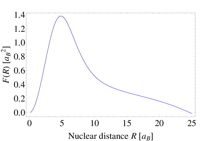
The function $M(R)$ may also be expressed as $M(R)=R^{2}(m_{1}^{2}+m_{2}^{2})/m_{12}^{2}+\langle z^{2}\rangle+\langle x^{2}\rangle$ (the angular brackets refer to the averaging over the electronic coordinates with $\psi_{1s\sigma}^{({\rm e)}}$). Note that $F(R)$ is independent of the molecular species and $M(R)$ is the same for all homonuclear species: $M(R)|_{m_{1}=m_{2}}=R^{2}/4+F(R)$. The function $F(R)$ , which gives the correction to the asymptotic behavior of $M(R)$, was introduced in [16]. In Fig. 1 we plot it.

References

• [1] J.C.J. Koelemeij, B. Roth, A. Wicht, I. Ernsting, and S. Schiller, Phys. Rev. Lett. 98, 173002 (2007).
• [2] U. Bressel, A. Borodin, J. Shen, M. Hansen, I. Ernsting, and S. Schiller, “Manipulation of Individual Hyperfine States in Cold Trapped Molecular Ions and Application to HD+\hbox{\rm HD}^{+} Frequency Metrology”, Phys. Rev. Lett. 108, 183003 (2012)
• [3] V. I. Korobov and Zhen-Xiang Zhong, “Bethe logarithm for the H2+\hbox{\rm H}_{2}^{+} and HD+\hbox{\rm HD}^{+} molecular ions”, Phys. Rev. A 86, 044501 (2012)
• [4] J.-P. Karr, A. Douillet, L. Hilico, “Photodissociation of trapped H2+\hbox{\rm H}_{2}^{+} ions for REMPD spectroscopy”, Appl. Phys. B 107, 1043–1052 (2012); DOI 10.1007/s00340-011-4757-z
• [5] A. K. Bekbaev, V. I. Korobov, and M. Dineykhan, “Variational calculations of the HT+\hbox{\rm HT}^{+} rovibrational energies”, Phys. Rev. A 83, 044501 (2011); DOI: 10.1103/PhysRevA.83.044501
• [6] U. Fröhlich, B. Roth, P. Antonini, C. Lämmerzahl, A. Wicht, S. Schiller, in Seminar on Astrophysics, Clocks and Fundamental Constants, E. Peik, S. Karshenboim, eds., Lecture Notes in Physics, Springer, 648, 297 (2004)
• [7] S. Schiller and V.I. Korobov, Phys. Rev. A 71, 032505 (2005).
• [8] M. Kajita, Phys. Rev. A 77, 012511 (2008);
• [9] D. Bakalov, V.I. Korobov and S. Schiller, “Precision spectroscopy of the molecular ion HD+\hbox{\rm HD}^{+}: control of Zeeman shifts”, Phys. Rev. A 82, 055401 (2010).
• [10] D. Bakalov, V.I. Korobov and S. Schiller, “Magnetic field effects in the transitions of the HD+\hbox{\rm HD}^{+} molecular ion and precision spectroscopy”, J. Phys. B: At. Mol. Opt. Phys. 44, 025003 (2011); Corrigendum: J. Phys. B: At. Mol. Opt. Phys. 45, 049501 (2012).
• [11] R.E. Moss, and L. Valenzano, “The dipole polarizability of the hydrogen molecular cation HD+\hbox{\rm HD}^{+} and other isotopomers”, Molec. Phys. 100, 1527 (2002).
• [12] J.-Ph. Karr, S. Kilic, and L. Hilico, “Energy levels and two-photon transition probabilities in the HD+\hbox{\rm HD}^{+} ion”, J. Phys. B: At. Mol. Opt. Phys. 38, 853 (2005).
• [13] J.C.J. Koelemeij, “Infrared dynamic polarizability of HD+\hbox{\rm HD}^{+} rovibrational states”, Phys. Chem. Chem. Phys. 13, 18844 (2011).
• [14] D. Bakalov and S. Schiller, “Static Stark effect in the molecular ion HD+\hbox{\rm HD}^{+}”, Hyperfine interact. 210, 25 (2012)
• [15] D. R. Bates and G. Poots, Proc. Phys. Soc. (London) Sec. A 66, 784 (1953)
• [16] J. M. Peek, A. Hashemi-Attar, and C. L. Beckel, J. Chem. Phys. 71, 5382 (1979)
• [17] A. G. Posen, A. Dalgarno, J. M. Peek, ”The quadrupole vibration-rotation transition probabilities of the molecular hydrogen ion”, At. Data and Nucl. Data Tables 28, 265-277 (1983)
• [18] H. O. Pilón and D. Baye, “Quadrupole transitions in the bound rotational–vibrational spectrum of the hydrogen molecular ion”, J. Phys. B: At. Mol. Opt. Phys. 45, 065101 (2012); doi:10.1088/0953-4075/45/6/065101
• [19] D. M. Bishop and B. Lam, “Vibrational polarizabilities for H2+\hbox{\rm H}_{2}^{+}, H2{}_{\mbox{2}} and N2{}_{\mbox{2}}”, Chem. Phys. Lett. 134, 283-287 (1987)
• [20] D. M. Bishop and B. Lam, “An analysis of the interaction between a distant point charge and H2+\hbox{\rm H}_{2}^{+}”, Mol. Phys. 65, 679-688 (1988)
• [21] A. K. Bhatia and R. J. Drachman, Phys. Rev. A 61, 032503 (2000)
• [22] H. O. Pilón, “Quadrupole transitions in the bound rotational-vibrational spectrum of the deuterium molecular ion”, arXiv:1302.5234v2
• [23] D. Bakalov and V.I. Korobov, “Hyperfine structure of antiprotonic helium energy levels”, Phys. Rev. A 57, 1662 (1998).
• [24] V.I. Korobov and D. Bakalov, Phys. Rev. Lett. 79, 3379 (1997).
• [25] A.R. Edmonds, Angular Momentum in Quantum, Mechanics (Princeton University Press, Princeton, 1957), p. 57
• [26] V.I. Korobov, D. Bakalov and H.J. Monkhorst, Phys. Rev. A 59, R919 (1999).
• [27] D. Bakalov, V.I. Korobov, and S. Schiller, “High-precision calculation of the hyperfine structure of the HD+\hbox{\rm HD}^{+} ion”, Phys. Rev. Lett. 97, 243001 (2006).
• [28] V.I. Korobov, Phys. Rev. A 77, 022509 (2008).
• [29] H. Wind, J. Chem. Phys. 42, 2371 (1965).
• [30] V.I. Korobov, Phys. Rev. A 74, 052506 (2006).
• [31] H. J. Montgomery, “One-electron wavefunctions. Accurate expectation values”, Chem. Phys. Lett. 50, 455-458 (1977); http://dx.doi.org/10.1016/0009-2614(77)80365-5
• [32] N. Huntemann, M. Okhapkin, B. Lipphardt, S. Weyers, Chr. Tamm, and E. Peik, “High-Accuracy Optical Clock Based on the Octupole Transition in 171Yb+”, Phys. Rev. Lett. 108, 090801 (2012)
• [33] Values of the hyperfine hamiltonian coefficients for v=5v=5 and L=5L=5 levels were computed by V. Korobov and A. Bekbaev (private communication). The rotational g-factors for these levels were extrapolated from those of lower levels.
• [34] J. Shen, A. Borodin, M. Hansen, and S. Schiller, Phys. Rev. A 85, 032519 (2012).
• [35] W. M. Itano, “External-Field Shifts of the 199Hg+ Optical Frequency Standard”, J. Res. Natl. Inst. Stand. Technol. 105, 829–837 (2000).
• [36] W. H. Oskay, S. A. Diddams, E. A. Donley, T. M. Fortier, T. P. Heavner, L. Hollberg, W. M. Itano, S. R. Jefferts, M. J. Delaney, K. Kim, F. Levi, T. E. Parker, and J. C. Bergquist, “Single-Atom Optical Clock with High Accuracy”, Phys. Rev. Lett. 97, 020801 (2006); DOI: 10.1103/Phys. Rev. Lett.97.020801.
• [37] In addition to the neglect of excited electronic states, the calculations in Ref. [14] were performed taking into account only intermediate states with 0≤v≤40\leq v\leq 4. Therefore, the polarisabilities of the v=4,v=4, L=2L=2 level given in that paper deviate from the “correct” (within the chosen approximation) values by up to 1 at.u.
• [38] V.I. Korobov, A. Bekbaev, S. Schiller, et al., in preparation.
• [39] D. Bakalov, K. Bakalova, V.I. Korobov, H. J. Monkhorst, I. Shimamura, Phys. Rev. A 57, 3370 (1998).
• [40] P.E. Knowles, G.A. Beer, G.R. Mason, et al., “Muon catalyzed fusion in 3-K solid deuterium”, Phys. Rev. A 56, 1970 (1998).