Lipschitz gradients for global optimization
in a
one-point-based partitioning scheme
Abstract
A global optimization problem is studied where the objective function is a multidimensional black-box function and its gradient satisfies the Lipschitz condition over a hyperinterval with an unknown Lipschitz constant . Different methods for solving this problem by using an a priori given estimate of , its adaptive estimates, and adaptive estimates of local Lipschitz constants are known in the literature. Recently, the authors have proposed a one-dimensional algorithm working with multiple estimates of the Lipschitz constant for (the existence of such an algorithm was a challenge for 15 years). In this paper, a new multidimensional geometric method evolving the ideas of this one-dimensional scheme and using an efficient one-point-based partitioning strategy is proposed. Numerical experiments executed on 800 multidimensional test functions demonstrate quite a promising performance in comparison with popular DIRECT-based methods.
Key Words: Global optimization, Lipschitz gradients, set of Lipschitz constants, geometric algorithms.
MSC classes: 65K05, 90C26, 90C56.
1 Introduction
Global optimization is an important part of numerical analysis (see, e.g., [33, 43, 44, 46]). It considers problems derived from complex industrial applications where the objective function to be minimized is defined over a hyperinterval , , and can be black-box, multiextremal, and requiring high computational resources for its evaluation (see, e.g., [1, 5, 27, 28, 33, 34, 41, 43, 46]). Solving efficiently this type of problems is a great challenge, since they present a high number of local minimizers (only a few of which can be global ones), often with extremely different values, and do not present a simple mathematical description of the global optima.
One of the natural and powerful (from both the theoretical and the applied points of view) assumptions on these problems is that the objective function has bounded slopes, i.e.,
| (1) |
where denotes, usually, the Euclidean norm (other norms can be also used, see, e.g., [12, 30]) and is the (unknown) Lipschitz constant. In this case, Lipschitz global optimization methods can be applied (see, e.g., [6, 17, 18, 34, 41, 43, 46] and the references given therein). They can be distinguished, for example, by the way in which information about the Lipschitz constant is obtained and by the strategy of exploration of the admissible region.
In the literature, there exist at least four approaches to specify the Lipschitz constant from (1): (i) it can be given a priori (see, e.g., [7, 6, 17]); (ii) its global estimate over the whole domain can be used (see, e.g., [18, 22, 34, 43]); (iii) local Lipschitz constants can be estimated (see, e.g., [21, 41, 35, 43]); (iv) several estimates of can be chosen from a set of possible values (see, e.g., [9, 10, 16, 19, 26, 40, 41]). In their work global optimization methods using multiple estimates of the Lipschitz constants have proved to be particularly attractive for studying applied problems (see, e.g., [4, 15, 16, 29, 32], other references can be found, e.g., in [23, 40]).
In exploring the multidimensional search domain, various adaptive partitioning strategies can be applied. For example, one-point-based algorithms subsequently subdivide the search region in smaller ones and evaluate the objective function at one point within each subregion (see, e.g., [8, 6, 10, 19, 38]). Partitions of the search domain into hyperintervals, based on evaluating the objective function at the two vertices corresponding to the main diagonal of hyperintervals called diagonal partitioning strategies, can also be successfully used (see, e.g.,[14, 21, 22, 34, 40, 41]). More complex partitions, based on simplices, auxiliary functions of various nature, and so on, have also been proposed (see, e.g., [18, 25, 45, 46]; many other references can be found in [42]).
The choice of the regions to be partitioned is based on an information about the objective function obtained during the search. It can be either of the probabilistic type (e.g., Bayesian approach applying the theory of random functions to a mathematical representation of available (certain or uncertain) a priori information on the objective function behavior, see, e.g., [20, 24, 28, 43, 46]), or of the deterministic one (e.g., geometric approach making a use of different auxiliary functions to estimate the behavior of over the search region, see, e.g., [2, 17, 18, 34, 41, 35, 36, 43, 46]).
In this paper, a particular class of the Lipschitz global optimization problems is considered, namely, the class of problems with differentiable objective functions having the Lipschitz gradients , i.e.,
| (2) |
| (3) |
where
| (4) |
It is supposed in this formulation that the objective function can be black-box, multiextremal, its gradient (which could be itself a costly multiextremal black-box vector-function) can be calculated during the search, and is Lipschitz-continuous with some fixed, but unknown, constant , , over . These problems are often encountered in engineering applications (see, e.g., [34, 41, 43]), particularly, in electrical engineering optimization problems (see, e.g., [39, 41, 43]).
In the literature, several methods for solving this problem have been proposed. They can be also distinguished, for instance, with respect to the way the Lipschitz constant is estimated in their work. There exist algorithms using an a priori given estimate of (see, e.g., [2, 3, 36]), its adaptive estimates (see, e.g., [14, 41, 36]), and adaptive estimates of local Lipschitz constants (see, e.g., [41, 36]). Algorithms working with a number of Lipschitz constants for chosen from a set of possible values varying from zero to infinity were not known till 2009 when such an algorithm for solving the one-dimensional problem (2)–(4) has been proposed in [23]. Its extension to the multidimensional case is not a trivial task in contrast to the DIRECT method (see [19]) proposed in 1993 for solving problems with the Lipschitz objective function.
The present paper solves this more than 15-year open problem of constructing multidimensional global optimization methods working with multiple estimates of the Lipschitz constants for . A new multidimensional geometric method for finding solutions to the problem (2)–(4) is introduced and studied here. It uses a new one-point-based partitioning strategy (see [41, 38]) and works with a number of estimates of the Lipschitz constant for . Such multiple (from zero to infinity) estimates of from (3) are used to calculate the lower bounds of the objective function over the hyperintervals of a current partition of the search domain and to produce new trial points (i.e., points at which both the objective function and its gradient are evaluated). In the framework of geometric algorithms, this kind of estimating the Lipschitz constant can be interpreted as examination of all admissible minorant functions during the current iteration of the algorithm without constructing a specific one. A particular attention in the new algorithm is given to the improvement of the current minimal function value (the so-called record value) in order to provide a faster convergence to a global minimizer. As demonstrated by extensive numerical experiments executed on 800 test functions from the differentiable GKLS test classes (see [13]), the usage of gradients allows one to obtain, as expected, an acceleration in comparison with the DIRECT-based methods.
The paper is organized as follows. In Section 2, a theoretical background of the new algorithm is presented. Section 3 is dedicated to the description of the algorithm and to its convergence analysis. Finally, Section 4 contains results of numerical experiments executed on 800 test functions.
2 Theoretical background
In this section, the main theoretical results, necessary for introducing the new algorithm, are obtained. First, a new partitioning strategy developed in the framework of the one-point-based partition approach is described. The second part presents a technique for estimating the lower bounds of the objective function over hyperintervals. The third part is dedicated to the introduction of a procedure for determining nondominated hyperintervals, i.e., hyperintervals having the smallest lower bound for some particular estimate of the Lipschitz constant for . They are candidates for partitioning at each iteration of the new method.
2.1 One-point-based partitioning strategy
In this section, a new efficient one-point-based partitioning scheme proposed in [38] (see also [41]) is considered which is based on a diagonal partitioning strategy from [41, 37]. In this scheme, the function and its gradient are evaluated only at one vertex (either or ) of the main diagonal of each hyperinterval of the current partition independently of the problem dimension (recall that performing each trial is a time-consuming operation).
Let us start the description of this scheme with a two-dimensional example shown in Fig. 1. In this Figure, partitions of the admissible region produced by the algorithm at several initial iterations are presented starting from the first trial at the point (it is supposed here that a single iteration consists of the subdivision of only one hyperinterval). Black dots represent the trial points and the numbers around these dots indicate iterations at which these trial points have been generated. The terms ‘interval’ and ‘subinterval’ will be used to denote two-dimensional rectangular domains.
In Fig. 1a, the situation after the first two iterations is presented. Particularly, at the second iteration, the interval is partitioned into three subintervals of equal area (equal volume in a general case). This subdivision is performed by two lines (hyperplanes) orthogonal to the longest edge of (see Fig. 1a). The trial (evaluation of the objective function and, as we propose in this paper, of its gradient) is performed only at the point denoted by number 2.
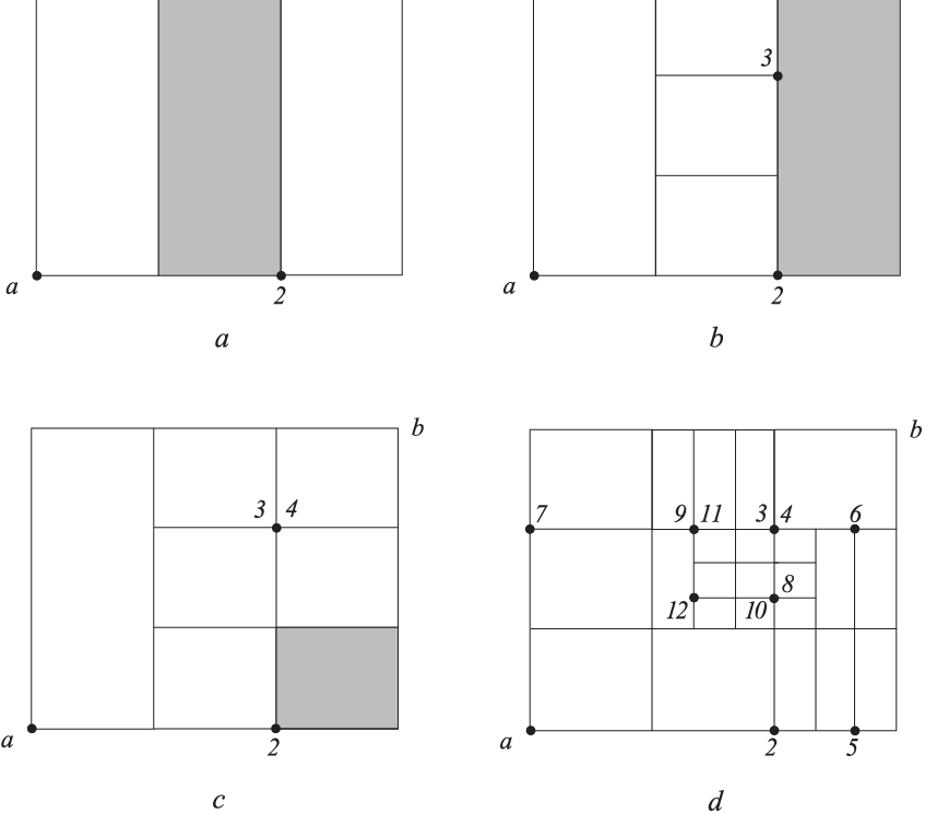
Let us suppose that the interval shown in light grey in Fig. 1a is chosen for the further partitioning. Thus, at the third iteration, three smaller subintervals are generated (see Fig. 1b). As one can see from Fig. 1c, the trial point of the fourth iteration coincides with the point 3 at which the trial has already been executed. Therefore, there is no need to perform a new (costly) evaluation of and at this point, since the values obtained at the previous iteration can be used. These values can be stored in a specially designed vertex database and is simply retrieved on demand without re-evaluations of the functions. For example, Fig. 1d illustrates the situation after 12 iterations. It can be seen from this figure that intervals have been generated by only 9 trial points.
Now we can describe the general scheme of a hyperinterval partitioning by assuming (without loss of generality) that the search hyperinterval in (4) is an -dimensional hypercube and the first trial is performed at the vertex (the scheme starting from the vertex is obtained analogously). Let a hyperinterval of a current partition of be chosen for partitioning at an iteration of the algorithm. The operation of partitioning the selected hyperinterval is performed as follows.
- Step 1.
-
Determine points and by the following formulae
(5) (6) where , and is given by the equation
(7) Get (evaluate or read from the vertex database) the values of the objective function and its gradient only at the point .
- Step 2.
-
Divide the hyperinterval into three hyperintervals of equal volume by two parallel hyperplanes that are perpendicular to the longest edge of and pass through the points and .
The hyperinterval is so substituted by three new hyperintervals with indices , , and (where is the number of hyperintervals at the beginning of the iteration ) determined by the vertices of their main diagonals
(8) (9) (10) Augment the current number of hyperintervals by 2.
From the partitioning scheme described above it can be observed that, contrary to many traditional partitioning strategies (see, e.g., [8, 14, 19, 21, 34]), the condition
does not have to be satisfied for all hyperintervals , and their main diagonals determined by the vertices and can be oriented in different ways. However, as theoretically shown in [41, 37], the hyperintervals orientations are not arbitrary and a special linking of hyperintervals generated at different iterations can be established with some efforts.
This smart linking will allow us to store information about vertices and the corresponding values of and in a special database, thereby avoiding redundant functions evaluations. The objective function and its gradient will be calculated at a vertex only once, stored in the database, and read when required. The new partitioning strategy generates trial points in such a regular way that one vertex where the functions are evaluated can belong to several (up to ) hyperintervals (see, for example, a trial point at the 8-th iteration in Fig. 1d). Therefore, the time-consuming operation of the functions evaluations is replaced by a significantly faster operation of reading (up to times) the functions values from the database. In this way, the new partitioning strategy considerably speeds up the search, especially when problems of high dimensions are considered (see [22, 37, 38]).
Note also that the possibility to choose the sequence of trial points among either the points or the points (or among other vertices) of hyperintervals (see Step 1 of the scheme) offers an important tool for accelerating the global search when some additional information about the objective function is known (we will see an example of this situation in Section 4). Note the center-sampling partitioning strategies (see, e.g., [8, 10, 19]) do not have this property.
2.2 Lower bounding
Let us consider an iteration of the new algorithm and a current partition of the search hyperinterval into hyperintervals , ; over these hyperintervals the values of both the function and its gradient are obtained (evaluated or read from the vertex database) at trial points , . In order to choose some hyperintervals for the further partition, the goodness (expressed by the so-called characteristic, see, e.g., [34, 41, 42, 43]) of the hyperintervals with respect to the global search is estimated by the algorithm. Better is the characteristic of a hyperinterval (in some predetermined sense), higher is the possibility to find the global minimizer within this hyperinterval. This hyperinterval is, therefore, a good candidate for a subdivision at the next iteration of the algorithm.
An estimate of the lower bound of over a hyperinterval is one of the possible characteristics of this hyperinterval. The following result holds.
Theorem 1
Let be an estimate of the Lipschitz constant for from (3), and be a hyperinterval of a current partition with a trial point . Then, a value of the characteristic of can be found such that it is the lower bound of over , i.e., , .
Proof 1
Let us prove the theorem in a constructive way. It is known (see, e.g., [8, 30, 31]) that for a differentiable function over a hyperinterval the following inequality is satisfied:
| (11) |
where the quadratic minorant function is defined over as
| (12) |
Here is the scalar product, is the Euclidean norm in , and
is the linear approximation of over .
From inequality (11) the following estimates can be obtained:
where is the minimum value of the linear approximation over , i.e.,
| (13) |
Since the function is linear, its minimum (13) is obtained in the vertex of the hyperinterval which coordinates , can be calculated as follows:
| (14) |
The corresponding value from (13) is therefore equal to
| (15) |
It is clear now that the value
| (16) |
satisfies the inequality
and, therefore, it can be taken as the characteristic value of that estimates the lower bound of over . The theorem has been proved.
Note that analogous results can be obtained in the case of hyperintervals with trial points rather than .

In Fig. 2, a quadratic minorant function from (12) is illustrated for over a hyperinterval . Here, the characteristic value coincides with the minimum value of obtained at the point of the main diagonal of . In general, as it can be seen from (12), the value is smaller than or equal to the minimum value of over .
2.3 Nondominated hyperintervals and their graphical representation
By using the obtained characteristics of hyperintervals, the relation of domination can be established between every two hyperintervals of a current partition of and a set of nondominated hyperintervals can be identified for a possible subdivision at the current iteration of the new algorithm (see [23, 40]).
Definition 1
Given an estimate of the Lipschitz constant from (3), a hyperinterval dominates a hyperinterval with respect to if
Definition 2
A hyperinterval is said to be nondominated with respect to if for the chosen value there is no other hyperinterval in which dominates .

Let us now generalize the approach proposed by the authors in [23] for the one-dimensional prototype and show that both a multi-dimensional interval of a current partition and the respective characteristic using the gradient can be represented in a two-dimensional diagram similar to those proposed in [19, 40] for derivative free methods. Difficulties in the construction of such a diagram were among the main reasons that prevented people to propose methods using several estimates of in their work.
So, we take for the dot, corresponding to , the vertical coordinate from (13)–(15) and the horizontal coordinate equal to half of the squared length of the main diagonal of , i.e.,
For example, in Fig. 3, a partition of the search domain consisting of three hyperintervals is represented by the dots , , and . Let us suppose that the Lipschitz constant for the gradient is estimated by , . The characteristic of a hyperinterval , , can be graphically obtained as the vertical coordinate of the intersection point of the line passed through the point with the slope and the vertical coordinate axis (see Fig. 3). It is easy to see, that with respect to the estimate the hyperinterval dominates both hyperintervals and and the hyperinterval dominates .
If a higher estimate of the Lipschitz constant is considered (see Fig. 3), the hyperinterval still dominates with respect to , because . But in its turn is dominated by the hyperinterval with respect to , because (see Fig. 3).
Since the exact Lipschitz constant for (or its valid overestimate) is unknown in the stated problem, the following definition can be useful.
Definition 3
A hyperinterval is called nondominated if there exists an estimate of the Lipschitz constant such that is nondominated with respect to .
This means that nondominated hyperintervals are those with the smallest characteristics (16) for some particular estimate of the Lipschitz constant for the gradient . For example, in Fig. 3 the hyperintervals and are nondominated.

It can be demonstrated following the reasoning used in [23, 40] that nondominated hyperintervals (in the sense of Def. 3) are located on the lower-right convex hull of the set of dots representing the hyperintervals of the current partition of and can be efficiently found by applying algorithm for identifying the convex hull of the dots (see, e.g., [16, 19, 41]). In Fig. 4, the hyperintervals represented by the dots (the largest hyperinterval), , , and are nondominated hyperintervals.
It has been shown in [40] that the hyperintervals of a current partition of form several groups characterized by the length of their main diagonals. The hyperintervals from a group are represented graphically by dots with the same horizontal coordinate. For example, in Fig. 4 there are seven different groups of hyperintervals with the horizontal coordinates equal to , , and one empty group (with the horizontal coordinate between and in Fig. 4). Empty groups correspond to hyperintervals which are not present in the current partition but can be generated (or were generated) at the successive (previous) iterations of the method.
As demonstrated in [40, 37], a correspondence between the length of the main diagonal of a hyperinterval and a non-negative integer number can be established, which indicates the number of subdivisions of the initial domain necessary to obtain the hyperinterval . At each iteration this number can be considered as an index of a group of equal hyperintervals where
| (17) |
and and are indices corresponding to the groups of the largest and smallest hyperintervals of the current partition of , respectively (for example, in Fig. 4, ). During partitioning, diagonals of hyperintervals become smaller, while the corresponding group indices grow up consecutively starting from (see [40] for details).
Once a nondominated hyperinterval is determined (with respect to some estimate of the Lipschitz constant ), it can be subdivided at the next iteration of the algorithm if the following condition is satisfied:
| (18) |
where is calculated by (16), is the record value, i.e., the current minimal function value (attained at the record point ), and is the parameter of the algorithm, (it can be set in different ways, see Section 4). Notice that both the record value and the record point can be changed after performing some better trial during partitioning, but the record value remains always greater than or equal to the vertical coordinate of the lowest dot (dot in Fig. 4).
Condition (18) prevents the algorithm from subdividing already well-explored small hyperintervals. For example, among nondominated hyperintervals in Fig. 4 (black dots), the hyperinterval does not satisfy this condition and therefore is excluded from being partitioned at the next iteration of the method.
It should be mentioned in this occasion that, together with nondominated hyperintervals, a hyperinterval containing the record point (called hereafter the record hyperinterval) is also considered for a possible partition during the work of the algorithm as it will be explained in the next Section. Among different hyperintervals the record point can belong to (up to ), the record hyperinterval is that with the smallest characteristic and can be changed during subdivisions. In Fig. 4, the record hyperinterval is represented by the dot (note that this dot can be not the lowest one, as in Fig. 4). Hereafter, the index of the group the hyperinterval belongs to will be indicated as (during the work of the algorithm the satisfaction of inequalities (17) is ensured for this index which can be eventually updated together with and ; see [40] for details). In Fig. 4, and, therefore, the hyperinterval is among the smallest hyperintervals of the illustrated partition of .
3 New Algorithm
In this Section, the new algorithm for solving problem (2)–(4) is described. First, the new method is presented and its computational scheme is given, then its convergence properties are analyzed.
The new algorithm consists of the following explicitly defined phases: (1) an exploration phase, at which an examination of large hyperintervals (possibly located far away from the record point) is performed in order to capture new subregions with better function values; (2) a record improvement phase, at which the algorithm tries to better inspect the subregion around the record point. Several subdivisions of different hyperintervals can be performed at a single iteration of the new method (this more general notion of an iteration with respect to that of Section 2.1 is often used in the Lipschitz global optimization algorithms with multiple estimates of Lipschitz constants, see, e.g., [10, 19, 23, 40]).
The exploration phase consists of several iterations (namely, where is the problem dimension), each serves for determining nondominated hyperintervals and partitioning them. Since each subdivision of a hyperinterval by the scheme (5)–(10) is performed perpendicularly to only one side of the hyperinterval (to the longest side from (7)), the number of iterations within a phase of the algorithm should be correlated with the hyperintervals dimension.
This phase is interrupted after finishing an iteration if an improvement on at least of the minimal function value is reached, i.e., if
| (19) |
where is the record value memorized at the start of the exploration phase.
Condition (19) is verified after each iteration of the exploration phase and is used to switch the algorithm to the record improvement phase. This local phase is also launched when the exploration phase finishes without having improved the record value, but only if the record hyperinterval is not the smallest one within the current partition of hyperintervals (for example, in Fig. 4, the record hyperinterval is among the smallest hyperintervals). Otherwise, the algorithm re-initiates another global exploration phase without forcing the local one.
The record improvement phase reflects the already well-established fact in global optimization affirming the benefits of the record improvement during the global search (see, e.g., the references given in [17, 23, 24, 41]). At a single iteration, it performs several subdivisions (namely, ) of the record hyperinterval trying to improve the record value. During this process a new record value can appear. In this case, a new record hyperinterval can be considered for remaining subdivisions.
The record hyperinterval subdivisions are performed by means of the one-point-based strategy described in Section 2.1. Of course, other possible local improvement techniques can be used for this scope (see, e.g., [11, 30, 31]) but in this case the resulting trial points can not be managed within the vertex database mentioned in Section 2.1.
It is important that the available gradient information allows us to terminate automatically the record improvement phase. In fact, the record hyperinterval is not further subdivided when the gradient projection on the directions parallel to the record hyperinterval sides becomes non-negative, i.e., when the following condition is satisfied:
| (20) |
Either in this case or when the prefixed number of subdivisions are normally performed (without meeting conditions (20)), the algorithm is switched again to the global exploration phase and continues its work.
The algorithm stops when the number of generated trial points reaches the maximal allowed number . The satisfaction of this termination criterion is verified after every subdivision of a hyperinterval. The current record value and the current record point can be taken as approximations of the global minimum value and the global minimizer from (2), respectively.
A formal description of the new algorithm follows below (we assume without loss of generality that the admissible region in (4) is an -dimensional hypercube).
-
Step 0 (Initialization). Set the iteration counter . Let the first evaluation of and be performed at the vertex of the initial hyperinterval , i.e., . Set the current partition of the search interval as , where , , and the current number of hyperintervals . Set , , and . Set group indices .
Suppose now that iterations of the algorithm have already been executed. The next iterations of the algorithm consist of the following steps.
-
Step 1 (Exploration Phase). Memorize the current record , set the counter of iterations during the exploration phase and perform the following steps:
- Step 1.1.
-
Identify the set of nondominated hyperintervals considering only groups of large hyperintervals (namely, those with the current indices from up to ). Subdivide those nondominated hyperintervals which satisfy inequality (18) and produce new trial points (or read the existing ones from the vertex database) according to Section 2.1. Set and update hyperintervals indices if necessary (see [40] for details).
- Step 1.2.
-
If condition (19) is satisfied, then go to Step 2 and execute the record improvement phase. Otherwise, go to Step 1.3.
- Step 1.3.
-
Increase the counter : check whether . If this is the case, then go to Step 1.1 (continue the exploration of large hyperintervals). Otherwise, go to Step 1.4 (perform the final iteration of the exploration phase by considering more hyperintervals groups).
- Step 1.4.
-
Identify the set of nondominated hyperintervals considering the current groups of hyperintervals from up to . Subdivide those nondominated hyperintervals which satisfy inequality (18) and produce new trial points (or read the existing ones from the vertex database) according to Section 2.1. Set , update all necessary indices.
- Step 1.5.
-
If the record hyperinterval is not the smallest one, i.e., if , then then go to Step 2 and execute the record improvement phase. Otherwise, go to Step 1 and repeat the exploration phase updating the value .
-
Step 2 (Record Improvement Phase). Set . Set the counter of iterations during the record improvement phase and perform the following steps:
- Step 2.1.
-
Subdivide the record hyperinterval and produce a new trial point (or read the existing one from the vertex database) according to Section 2.1. Update hyperintervals indices and the record hyperinterval index if necessary.
- Step 2.2.
-
Increase the counter : check whether . If this is the case, then go to Step 1 (perform a new exploration of large hyperintervals). Otherwise, go to Step 2.1 (continue the local exploration of the subregion near to the record point).
Let us now study convergence properties of the new method during minimization of the function from (2)–(4) when the maximal allowed number of generated trial points is equal to infinity. In this case, the algorithm does not stop (the number of iterations goes to infinity) and an infinite sequence of trial points is generated.
Definition 4
The convergence of an infinite sequence of trial points generated by a global optimization method is called everywhere dense if for any point and any there exist an iteration number and a point , , such that .
Theorem 2
The new algorithm manifests the everywhere dense convergence.
Proof 2
Every subdivision of a hyperinterval by the partitioning scheme from Section 2.1 produces three new hyperintervals with the same volume equal to the third part of the volume of the subdivided hyperinterval and smaller main diagonals. Trial points generated by the new algorithm are at one of the vertices of each generated hyperinterval. Therefore, fixed a positive value of , it is sufficient to demonstrate that after a finite number of iterations , the largest hyperinterval of the current partition of the search domain will have the length of its main diagonal smaller than . In this case, in -neighborhood of any point of there will exist at least one trial point generated by the algorithm.
Let us fix an iteration of the method and consider the group of the largest hyperintervals of the partition on its two-dimensional graphic representation. This group is always taken into account when nondominated hyperintervals are looked for at the exploration phase of the algorithm. As it follows from Def. 3, a hyperinterval from this group with the corresponding smallest value from (13)–(15), must be partitioned and substituted by three smaller hyperintervals at the current iteration of the algorithm because it is a nondominated hyperinterval and condition (18) is satisfied for it.
Since each group consists of a finite number of hyperintervals, after a sufficiently large number of iterations all hyperintervals of the group of the largest hyperintervals will be subdivided. The group index will increase and the same procedure will be repeated with a new group of the largest hyperintervals, thus making the largest hyperintervals smaller and smaller.
It can be also noted that the record hyperinterval is itself represented by a dot in the two-dimensional diagram of the current partition. It can be subdivided either separately during the record improvement phase, or as a nondominated hyperinterval during the exploration phase at which the satisfaction of condition (20) is not taken in consideration.
Thus, there exists a finite number such that after executing iterations of the algorithm the largest hyperinterval of the current partition will have the main diagonal smaller than .
To conclude the theoretical study of the new algorithm we would like to highlight that the usage of all possible estimates of the Lipschitz constant in its work leads to the convergence of the everywhere dense type. If the Lipschitz constant (or its valid estimate) of the objective function or the Lipschitz constant (or its valid estimate) of the gradient can be used by a global optimization method, other types of convergence can be established for such an algorithm (see, e.g., methods from [18, 34, 41, 42, 43]).
4 Numerical results
In this Section, we present numerical results performed to compare the new algorithm with two methods belonging to the same class of the one-point-base partitioning methods: the DIRECT algorithm from [19] and its locally-biased modification DIRECTl from [10]. Both of them use the center-sampling partitioning strategy and work with a set of Lipschitz constants for the objective function from (2). The implementation of these two methods (downloadable from http://www4.ncsu.edu/~ctk/SOFTWARE/DIRECTv204.tar.gz) has been used in all the experiments following the way of the multicriteria comparison proposed in [40].
In order to make easier the numerical comparison with the DIRECT-based algorithms, the value from (18) was set as in the DIRECT method, i.e.,
| (21) |
In accordance with [40], the global minimizer was considered to be found when a method generated a trial point inside a hyperinterval with a vertex and the volume smaller than the volume of the initial hyperinterval multiplied by an accuracy coefficient , , i.e.,
| (22) |
where is from (4). The algorithm was stopped either when the maximal number of trials equal to 1 000 000 was reached, or when condition (22) was satisfied (see [40] for a discussion about different stopping criteria in global optimization methods).
In our numerical experiments we used the same test classes, each of 100 continuously differentiable functions, produced by the GKLS-generator (see [13]) as in [40]. Particularly, eight GKLS D-type classes of dimensions , 3, 4, and 5 have been considered. For each particular problem dimension a ‘simple’ and a ‘hard’ classes have been taken for the comparison (see [40] for a detailed description of the classes).
For the convenience of the reader, we report here the four criteria introduced in [40, 41] that were used to compare the methods. The following designations are required:
– the number of trials performed by the method under consideration to solve the problem number , , of a fixed test class.
– the number of hyperintervals generated to solve the problem .
Criterion C1. Number of trials required for a method to satisfy condition (22) for all 100 functions of a particular test class, i.e.,
| (23) |
Criterion C2. The corresponding number of hyperintervals, , generated by the method, where is from (23).
Criterion C3. Average number of trials performed by the method during minimization of all 100 functions from a particular test class, i.e.,
| (24) |
Criterion C4. Number (number ) of functions from a class for which DIRECT or DIRECTl executed less (more) function evaluations than the new algorithm. If is the number of trials performed by the new algorithm and is the corresponding number of trials performed by a competing method, and are evaluated as follows
| (25) |
| (26) |
Results based on Criteria C1 and C2 are mainly influenced by minimization of the most difficult functions of a class. Criteria C3 and C4 deal with average data of a class. The number of generated hyperintervals (Criterion C2) provides an important characteristic of any partition algorithm for solving the problem (2)–(4). In some way, it corresponds to the qualitative examination of the search domain during the work of the method. The greater is this number, the more information about the behavior of the objective function is available and, therefore, the smaller is the risk to miss its global minimizer. Of course, algorithms should not generate many redundant hyperintervals since this slows down the search and is therefore a disadvantage of the method (see [40] for more details).
Results of numerical comparison of the methods with respect to Criteria C1 and C2 with eight GKLS test classes are shown in Tables 1–3. The accuracy coefficient from (22) is given in the second column of the tables. Table 1 reports the maximal number of trials required for satisfying condition (22) for half of the functions of a particular class (columns “50%”) and for all 100 function of the class (columns “100%”). The notation ‘ 1 000 000 ’ in Tables 1 and 3 means that after 1 000 000 function evaluations the method under consideration was not able to solve problems. Table 2 represents the ratio between the maximal number of trials performed by DIRECT and DIRECTl with respect to the corresponding number of trials performed by the new algorithm. The numbers of generated hyperintervals (Criterion C2) are indicated in Table 3.
According to Tables 1 and 3, the new multidimensional algorithm requires much fewer trials than the other two methods to ensure a thorough examination of the search domain. Moreover, the advantage of the new method becomes even more pronounced as the problem dimension grows or the problem complexity increases.
In fact, on half of the test functions from each class (which were the most simple for each method with respect to the other functions of the class) the new algorithm already manifested a very good performance with respect to DIRECT and DIRECTl in terms of the number of generated trial points (see columns “50%” in Table 1). When all the functions were taken in consideration (and, consequently, difficult functions of the class were considered too), the number of trials produced by the new algorithm was much fewer in comparison with two other methods (see columns “100%” in Table 1), ensuring at the same time a substantial examination of the admissible domain (see Table 3).
| Class | 50% | 100% | ||||||
|---|---|---|---|---|---|---|---|---|
| DIRECT | DIRECTl | New | DIRECT | DIRECTl | New | |||
| 2 | simple | 111 | 152 | 59 | 1159 | 2318 | 335 | |
| 2 | hard | 1062 | 1328 | 182 | 3201 | 3414 | 1075 | |
| 3 | simple | 386 | 591 | 362 | 12507 | 13309 | 2043 | |
| 3 | hard | 1749 | 1967 | 416 | 1000000 (4) | 29233 | 2352 | |
| 4 | simple | 4805 | 7194 | 2574 | 1000000 (4) | 118744 | 16976 | |
| 4 | hard | 16114 | 33147 | 3773 | 1000000 (7) | 287857 | 20866 | |
| 5 | simple | 1660 | 9246 | 1757 | 1000000 (1) | 178217 | 16300 | |
| 5 | hard | 55092 | 126304 | 13662 | 1000000 (16) | 1000000 (4) | 88459 | |
| Class | DIRECT/New | DIRECTl/New | ||
| 2 | simple | 3.46 | 6.92 | |
| 2 | hard | 2.98 | 3.18 | |
| 3 | simple | 6.12 | 6.51 | |
| 3 | hard | 425.17 | 12.43 | |
| 4 | simple | 58.91 | 6.99 | |
| 4 | hard | 47.92 | 13.80 | |
| 5 | simple | 61.35 | 10.93 | |
| 5 | hard | 11.30 | 11.30 |
Note also that maximal number of trials equal to 88459 (see Table 1) required by the new method to solve all problems of the hard five-dimensional class is obtained on the function 5 of this class. If we use the new method with the one-point-based strategy starting from the point rather than from the point (see Section 2.1), the number of trials required by the new algorithm to solve this particular problem becomes equal to . Thus, some a priori knowledge on the objective function behavior can allow us to better select the vertex of the initial hyperinterval in which the first trial will be executed and, therefore, to accelerate the search even more.
Table 4 reports the average number of trials performed during minimization of all 100 functions from the same GKLS classes (Criterion C3). The “Improvement” columns in these tables represent the ratios between the average numbers of trials performed by DIRECT and DIRECTl with respect to the corresponding numbers of trials performed by the new algorithm. The symbol ‘’ reflects the situation when not all functions of a class were successfully minimized by the method under consideration in the sense of condition (22). This means that the method stopped when trials had been executed during minimization of several functions of this particular test class. In these cases, the value of equal to 1 000 000 was used in calculations of the average value in (24), providing in such a way a lower estimate of the average. As can be seen from Table 4, the new method outperforms DIRECT and DIRECTl also on Criterion C3.
| Class | 50% | 100% | ||||||
|---|---|---|---|---|---|---|---|---|
| DIRECT | DIRECTl | New | DIRECT | DIRECTl | New | |||
| 2 | simple | 111 | 152 | 185 | 1159 | 2318 | 1137 | |
| 2 | hard | 1062 | 1328 | 607 | 3201 | 3414 | 3993 | |
| 3 | simple | 386 | 591 | 1867 | 12507 | 13309 | 12149 | |
| 3 | hard | 1749 | 1967 | 2061 | 1000000 (4) | 29233 | 14357 | |
| 4 | simple | 4805 | 7194 | 21635 | 1000000 (4) | 118744 | 186295 | |
| 4 | hard | 16114 | 33147 | 33173 | 1000000 (7) | 287857 | 223263 | |
| 5 | simple | 1660 | 9246 | 19823 | 1000000 (1) | 178217 | 255059 | |
| 5 | hard | 55092 | 126304 | 169413 | 1000000 (16) | 1000000 (4) | 1592969 | |
| Class | DIRECT | DIRECTl | New | Improvement | |||
| DIRECT/New | DIRECTl/New | ||||||
| 2 | simple | 198.89 | 292.79 | 97.22 | 2.06 | 3.01 | |
| 2 | hard | 1063.78 | 1267.07 | 192.00 | 5.54 | 6.60 | |
| 3 | simple | 1117.70 | 1785.73 | 491.28 | 2.28 | 3.63 | |
| 3 | hard | 42322.65 | 4858.93 | 618.32 | 68.45 | 7.86 | |
| 4 | simple | 47282.89 | 18983.55 | 3675.84 | 12.87 | 5.16 | |
| 4 | hard | 95708.25 | 68754.02 | 5524.77 | 17.32 | 12.44 | |
| 5 | simple | 16057.46 | 16758.44 | 3759.05 | 4.27 | 4.46 | |
| 5 | hard | 217215.58 | 269064.35 | 22189.47 | 9.79 | 12.13 | |
Finally, results of comparison between the new algorithm and its two competitors in terms of Criterion C4 are reported in Table 5. This table shows how often the new algorithm was able to minimize each of 100 functions of a class with a smaller number of trials with respect to DIRECT or DIRECTl. The notation ‘ : ’ means that among 100 functions of a particular test class there are functions for which DIRECT (or DIRECTl) spent fewer function trials than the new algorithm and functions for which the new algorithm generated fewer trial points with respect to DIRECT (or DIRECTl) ( and are from (25) and (26), respectively). As a rule, the more hard objective functions are presented in a test class, the more pronounced becomes the advantage of the new algorithm on Criterion C4, as well.
| Class | DIRECT : New | DIRECTl : New | ||
|---|---|---|---|---|
| 2 | simple | 28 : 72 | 21 : 79 | |
| 2 | hard | 15 : 85 | 16 : 84 | |
| 3 | simple | 36 : 64 | 30 : 70 | |
| 3 | hard | 19 : 81 | 17 : 83 | |
| 4 | simple | 39 : 61 | 25 : 75 | |
| 4 | hard | 14 : 86 | 16 : 84 | |
| 5 | simple | 55 : 45 | 17 : 83 | |
| 5 | hard | 26 : 74 | 20 : 80 |
As demonstrated by the results of the extensive numerical experiments performed, the usage of the gradient information together with the efficient partitioning strategy allows one to obtain a serious acceleration in comparison with the DIRECT-based methods on the studied classes of test problems.
References
- [1] C. Audet, P. Hansen, and G. Savard (eds.), Essays and surveys in global optimization, GERAD 25th Anniversary, Springer–Verlag, New York, 2005.
- [2] W. Baritompa, Customizing methods for global optimization – A geometric viewpoint, J. Global Optim. 3 (1993), no. 2, 193–212.
- [3] L. Breiman and A. Cutler, A deterministic algorithm for global optimization, Math. Program. 58 (1993), no. 1–3, 179–199.
- [4] D. Di Serafino, G. Liuzzi, V. Piccialli, F. Riccio, and G. Toraldo, A modified DIviding RECTangles algorithm for a problem in astrophysics, J. Optim. Theory Appl. 151 (2011), no. 1, 175–190.
- [5] L. Dumas, B. Druez, and N. Lecerf, A fully adaptive hybrid optimization of aircraft engine blades, J. Comput. Appl. Math. 232 (2009), no. 1, 54–60.
- [6] Yu. G. Evtushenko, Numerical optimization techniques, Translations Series in Mathematics and Engineering, Springer–Verlag, Berlin, 1985.
- [7] Yu. G. Evtushenko, V. U. Malkova, and A. A. Stanevichyus, Parallel global optimization of functions of several variables, Comput. Math. Math. Phys. 49 (2009), no. 2, 246–260.
- [8] Yu. G. Evtushenko and M. A. Posypkin, An application of the nonuniform covering method to global optimization of mixed integer nonlinear problems, Comput. Math. Math. Phys. 51 (2011), no. 8, 1286–1298.
- [9] D. E. Finkel and C. T. Kelley, Additive scaling and the DIRECT algorithm, J. Global Optim. 36 (2006), no. 4, 597–608.
- [10] J. M. Gablonsky and C. T. Kelley, A locally-biased form of the DIRECT algorithm, J. Global Optim. 21 (2001), no. 1, 27–37.
- [11] M. Gaviano and D. Lera, A complexity analysis of local search algorithms in global optimization, Optim. Methods Softw. 17 (2002), no. 1, 113–127.
- [12] , A global minimization algorithm for Lipschitz functions, Optim. Lett. 2 (2008), no. 1, 1–13.
- [13] M. Gaviano, D. Lera, D. E. Kvasov, and Ya. D. Sergeyev, Algorithm 829: Software for generation of classes of test functions with known local and global minima for global optimization, ACM Trans. Math. Software 29 (2003), no. 4, 469–480.
- [14] V. P. Gergel, A global optimization algorithm for multivariate function with Lipschitzian first derivatives, J. Global Optim. 10 (1997), no. 3, 257–281.
- [15] P. A. Graf, K. Kim, W. B. Jones, and L.-W. Wang, Surface passivation optimization using DIRECT, J. Comput. Phys. 224 (2007), no. 2, 824–835.
- [16] J. He, L. T. Watson, N. Ramakrishnan, C. A. Shaffer, A. Verstak, J. Jiang, K. Bae, and W. H. Tranter, Dynamic data structures for a direct search algorithm, Comput. Optim. Appl. 23 (2002), no. 1, 5–25.
- [17] R. Horst and P. M. Pardalos (eds.), Handbook of global optimization, vol. 1, Kluwer Academic Publishers, Dordrecht, 1995.
- [18] R. Horst and H. Tuy, Global optimization – deterministic approaches, Springer–Verlag, Berlin, 1996.
- [19] D. R. Jones, C. D. Perttunen, and B. E. Stuckman, Lipschitzian optimization without the Lipschitz constant, J. Optim. Theory Appl. 79 (1993), no. 1, 157–181.
- [20] D. R. Jones, M. Schonlau, and W. J. Welch, Efficient global optimization of expensive black-box functions, J. Global Optim. 13 (1998), no. 4, 455–492.
- [21] D. E. Kvasov, C. Pizzuti, and Ya. D. Sergeyev, Local tuning and partition strategies for diagonal GO methods, Numer. Math. 94 (2003), no. 1, 93–106.
- [22] D. E. Kvasov and Ya. D. Sergeyev, Multidimensional global optimization algorithm based on adaptive diagonal curves, Comput. Math. Math. Phys. 43 (2003), no. 1, 42–59.
- [23] , A univariate global search working with a set of Lipschitz constants for the first derivative, Optim. Lett. 3 (2009), no. 2, 303–318.
- [24] D. Lera and Ya. D. Sergeyev, An information global minimization algorithm using the local improvement technique, J. Global Optim. 48 (2010), no. 1, 99–112.
- [25] , Lipschitz and Hölder global optimization using space-filling curves, Appl. Numer. Math. 60 (2010), no. 1–2, 115–129.
- [26] G. Liuzzi, S. Lucidi, and V. Piccialli, A partition-based global optimization algorithm, J. Global Optim. 48 (2010), no. 1, 113–128.
- [27] C. Luo, S.-L. Zhang, C. Wang, and Z. Jiang, A metamodel-assisted evolutionary algorithm for expensive optimization, J. Comput. Appl. Math. 236 (2011), no. 5, 759–764.
- [28] J. Mockus, A set of examples of global and discrete optimization: Applications of bayesian heuristic approach, Kluwer Academic Publishers, Dordrecht, 2000.
- [29] C. G. Moles, P. Mendes, and J. R. Banga, Parameter estimation in biochemical pathways: A comparison of global optimization methods, Genome Res. 13 (2003), no. 11, 2467–2474.
- [30] Yu. Nesterov, Introductory lectures on convex optimization: A Basic course, Kluwer Academic Publishers, Dordrecht, 2004.
- [31] J. Nocedal and S. J. Wright, Numerical optimization, Springer–Verlag, Dordrecht, 1999.
- [32] T. D. Panning, L. T. Watson, N. A. Allen, K. C. Chen, C. A. Shaffer, and J. J. Tyson, Deterministic parallel global parameter estimation for a model of the budding yeast cell cycle, J. Global Optim. 40 (2008), no. 4, 719–738.
- [33] P. M. Pardalos, H. E. Romeijn, and H. Tuy, Recent developments and trends in global optimization, J. Comput. Appl. Math. 124 (2000), no. 1-2, 209–228.
- [34] J. Pintér, Global optimization in action (continuous and lipschitz optimization: Algorithms, implementations and applications), Kluwer Academic Publishers, Dordrecht, 1996.
- [35] Ya. D. Sergeyev, An information global optimization algorithm with local tuning, SIAM J. Optim. 5 (1995), no. 4, 858–870.
- [36] , Global one-dimensional optimization using smooth auxiliary functions, Math. Program. 81 (1998), no. 1, 127–146.
- [37] , An efficient strategy for adaptive partition of -dimensional intervals in the framework of diagonal algorithms, J. Optim. Theory Appl. 107 (2000), no. 1, 145–168.
- [38] , Efficient partition of -dimensional intervals in the framework of one-point-based algorithms, J. Optim. Theory Appl. 124 (2005), no. 2, 503–510.
- [39] Ya. D. Sergeyev, P. Daponte, D. Grimaldi, and A. Molinaro, Two methods for solving optimization problems arising in electronic measurements and electrical engineering, SIAM J. Optim. 10 (1999), no. 1, 1–21.
- [40] Ya. D. Sergeyev and D. E. Kvasov, Global search based on efficient diagonal partitions and a set of Lipschitz constants, SIAM J. Optim. 16 (2006), no. 3, 910–937.
- [41] , Diagonal global optimization methods, FizMatLit, Moscow, 2008, In Russian.
- [42] Ya. D. Sergeyev and D. E. Kvasov, Lipschitz global optimization, Wiley Encyclopedia of Operations Research and Management Science (J. J. Cochran, ed.), vol. 4, Wiley, New York, 2011, pp. 2812–2828.
- [43] R. G. Strongin and Ya. D. Sergeyev, Global optimization with non-convex constraints: Sequential and parallel algorithms, Kluwer Academic Publishers, Dordrecht, 2000.
- [44] D. Trigiante (ed.), Recent trends in numerical analysis, Nova Science Publishers, Inc., New York, 2000.
- [45] Y. Wu, L. Ozdamar, and A. Kumar, TRIOPT: A triangulation-based partitioning algorithm for global optimization, J. Comput. Appl. Math. 177 (2005), no. 1, 35–53.
- [46] A. A. Zhigljavsky and A. Žilinskas, Stochastic global optimization, Springer, New York, 2008.