Boosting work characteristics and overall heat engine performance via shortcuts to adiabaticity: quantum and classical systems
Abstract
Under a general framework, shortcuts to adiabatic processes are shown to be possible in classical systems. We then study the distribution function of the work done on a small system initially prepared at thermal equilibrium. It is found that the work fluctuations can be significantly reduced via shortcuts to adiabatic processes. For example, in the classical case probabilities of having very large or almost zero work values are suppressed. In the quantum case negative work may be totally removed from the otherwise non-positive-definite work values. We also apply our findings to a micro Otto-cycle-based heat engine. It is shown that the use of shortcuts, which directly enhances the engine output power, can also increase the heat engine efficiency substantially, in both quantum and classical regimes.
pacs
03.65.-w, 45.20.Jj, 37.90.+jI Introduction
Shortcuts to adiabatic processes (STA) constitute a timely topic of broad interest [1, 2, 3, 4, 5, 6, 7, 8, 9, 10, 11, 12, 13], with several experimental realizations reported recently [7, 8, 9]. One important question follows: are such STA unique in quantum mechanics?
In this work, we first develop a simple and general framework for classical STA. Analogous to the classical adiabatic theorem, the involved Hamiltonian is assumed to be integrable [14]. A generic control field to achieve classical STA is then found. This is important because (i) classical STA may help to design quantum STA (e.g., by quantizing the classical control field) and (ii) STA may be more general and robust than previously thought. Indeed, applying our formalism to a parametric oscillator, the control Hamiltonian is precisely the classical limit of an early quantum result [15].
To make a new connection between STA and nonequilibrium statistical mechanics, we ask how STA impact the distribution function of the work done on a single system initially prepared in thermal equilibrium. We find that the work fluctuations can be significantly reduced. For example, both the long-tail part and the almost zero part of the work function in a classical example are substantially suppressed, leading to a faster convergence towards Jarzynski’s equality. Remarkably, in the corresponding quantum case negative work values of the otherwise non-positive-definite quantum work may be removed completely. We then show how STA implemented in a prototype micro heat engine [16, 17] can increase engine efficiency and the power output at the same time.
II Shortcuts to adiabatic processes: from quantum to classical systems
Consider first STA for a quantum system (also called transitionless driving in Ref. [2]) for a quantum system with a non-degenerate Hamiltonian , parameterized by , with the -th instantaneous energy eigenstate given by possessing eigenenergy . The quantum adiabatic theorem states that, if changes slowly enough, the system initially prepared on an eigenstate will continue to stay on the instantaneous energy eigenstate , i.e.,
| (1) |
where is the unitary time evolution operator, and includes a dynamical phase and a geometrical phase [18]. This solution clearly indicates the invariance of population on each instantaneous eigenstate. Such type of time evolution can be accelerated by adding a control Hamiltonian . In particular, by reverse engineering [1, 2] one finds
| (2) |
This assists an adiabatic process associated with (the process is certainly non-adiabatic with respect to the full Hamiltonian ), regardless of how fast varies. Note that [1, 2]. In the limit , also approaches zero and the quantum adiabatic theorem is recovered.
We now show that classical adiabatic processes also have shortcuts [19, 12], and the physics is analogous to the above quantum picture. Though our treatment applies to arbitrary multi-dimensional integrable classical systems, for convenience we consider here a time-dependent classical Hamiltonian with one degree of freedom [ are phase space variables]. To study classical adiabatic processes we further assume that at a fixed can be written as : a function of the action variable but not a function of the angle variable [20]. For a general time-dependent , the correct Hamiltonian in the action-angle representation is obtained by use of a time-dependent type-II generating function between and [20], i.e.,
| (3) |
Classical adiabatic theorem then states that is approximately a constant if is changing slowly.
To realize classical STA, i.e., to have a constant with fast changes in , we construct a control Hamiltonian on top of . One obvious but exact solution is
| (4) |
The total Hamiltonian then becomes
| (5) |
which is -independent, and as such is a constant of motion exactly. Note that . In the limit (), the classical adiabatic theorem is recovered. The theoretical result here is consistent with the above quantum STA result also because is an analog of the quantum number .
III Classical versus quantum work fluctuations
For a small system under a control protocol, the work done on a system fluctuates. To study the impact of STA [which establishes a constant (constant ) in classical (quantum) cases] on the work statistics, we introduce work functions below and advocate a useful scheme to connect STA with nonequilibrium statistical mechanics.
For a classical system initially prepared at , the inclusive work [21, 22, 23] during a period of is given by
| (6) |
where represents a classical trajectory emanating from . The classical work function is defined as
| (7) |
where describes the initial statistical ensemble, e.g., the Gibbs distribution corrsponding to . To have a fair comparison with the bare cases without , we propose a scheme in which and hence
| (8) |
That is, when evaluating the work, the control Hamiltonian does not directly affect the calculation because vanishes in the beginning and in the end. On the other hand, the trajectories are affected by and the work done to the system is now achieved by both a device achieving and by a field implementing . Interestingly, under our control scheme, the Jarzynski’s equality [21, 23], i.e.,
| (9) |
still holds for the same even with . Note that here represents the thermal average, and is the free energy difference between a thermal equilibrium state of the final-state configuration (at the same temperature) and the initial thermal state.
A comparison between classical and quantum work fluctuations will be stimulating. To that end we adopt the two-time measurement definition of quantum work [24], which is known as with and being the energy values upon energy measurement. The quantum work function is then given by
| (10) |
where is the initial probability on and is the transition probability between and . Adopting the same scheme as in classical cases i.e., , we have
| (11) |
IV Applications to a parametric oscillator
A parametric oscillator is feasible for experimental investigations [16, 17]. We are thus motivated to consider a parametric oscillator with a time-dependent angular frequency . In the quantum version, the Hamiltonian is
| (12) |
The required used to realize quantum transitionless driving is found to be [15]
| (13) |
which is proportional to . Such a control Hamiltonian may be realized by considering a magnetic field, whose vector potential is proportional to (this also effectively changes ). In the classical domain, the classical Hamiltonian is
| (14) |
Using our general result above one finds
| (15) |
Detailed calculations in the Appendix [19] show
| (16) |
which is precisely the classical limit of the quantum .
For work fluctuations we consider the classical case first. Because and we have set , we find and , with being an exact constant of motion under . The work expression then reduces to
| (17) | |||||
with taken to be positive. For simplicity we also denote and . Assuming that the system is initially prepared in a canonical distribution with inverse temperature , i.e.,
| (18) |
we obtain
| (19) |
with being the unit step function. Because this result is independent of details of , it does apply to conventional adiabatic cases as well. That is, the work function for STA remains identical with that in conventional adiabatic processes [25].
It is necessary and interesting to compare with the work function of a process with the same time-dependence of but without . For the bare protocol we obtain
| (20) | |||||
where is the modified Bessel function of the first kind with parameter . Here we have further assumed an (positive-valued) angular frequency increasing monotonically during the protocol, with a simple proof of the positive-definiteness of detailed in the Appendix. The constant factors should be determined by specific realizations of . In particular, in the sudden change limit (SL) of , reduces to
| (21) |
Interestingly, diverges at whereas is always finite. Equally interesting, since we assume (without loss of generality), we have
| (22) |
So the exponential decay rate of , which is , is less than half of the exponential decay rate of for STA. Two main impacts of STA on the work function are hence clear: the probabilities for both very small and large work values are strongly suppressed.
To illustrate and corroborate our analysis we present in Fig. 1 numerical results of the work function. The results agree with our theoretical calculations. Indeed, compared with a bare protocol of the same duration, the STA case (i) suppresses the long tail of the work distribution and (ii) also significantly decreases the weights of almost zero work. Quantitatively, in terms of mean work and the standard deviation of work ,
| (23) |
for STA, whereas for a nonadiabatic process in the sudden change limit, we find
| (24) |
and a larger work variance
| (25) |
Certainly, suppressing the probabilities for small and large can be more significant than what is manifested in . To stress this point, we display in Fig. 2 a typical result converging towards Jarzynski’s equality with a limited number of classical simulation trajectories. It is seen that in either the bare protocol or the STA converges towards the same theoretical value, but the STA case does converge faster (statistically). This is an intriguing consequence of work fluctuation suppression. Indeed, the dissipated work, i.e., is also suppressed via STA. STA hence mimic the so-termed escorted free energy simulations put forward in Ref. [26]. Note, however, that here we use a strictly Hamiltonian control term which not only renders the validity of the Jarzynski equality but (in contrast to Ref. [26]) leaves the expression for physical work unchanged as well.

Let us now turn to the quantum work fluctuations with the initial quantum state at thermal equilibrium. Using Eq. (10) one finds that in STA or normal adiabatic processes,
| (26) |
with
| (27) |
The discrete sum is due to quantization. For general nonadiabatic processes without , analytical but rather complicated work functions are available [27, 28, 29]. Here we perform direct numerical investigations with a specific realization of considered in Figs. 1 and 2.
Our results in Fig. 3 show that the long tail distribution of quantum work is also strongly suppressed in STA, with the degree of suppression in good correspondence with our classical results. Quantitatively, for the parameters in Fig. 3, the work variance () in the STA (bare nonadiabatic) case. There are two other inspiring aspects. First, in the classical protocol (STA or a bare process) and in the quantum STA, is strictly positive-definite with monotonically increasing . In distinct contrast, however, in a bare quantum processes (i.e. without ), work attains an appreciable probability of becoming negative. Second, while for STA assumes equally spaced, discretized values only, in the bare processes work assumes a rich variety of different discrete values. It is also checked that via quantum Jarzynski’s equality the bare protocol and the STA indeed yield the same quantum .
V Enhancement in efficiency and power of a prototype micro heat engine
We now consider an Otto-cycle based heat engine using a parametric oscillator as its working medium [16, 17]. This involves -changing strokes without a reservoir (steps 1, 3) and two relaxation processes with reservoirs at two different inverse temperatures and (steps 2, 4). For the details of the four steps, see, e.g., Ref. [17].
It is convenient to assume steps 1 and 3 to be conventional (quasi) adiabatic or extremely nonadiabatic (sudden change limit) processes. With , , and the duration of each cycle step fixed, can be optimized to maximize the net work output, with the corresponding engine efficiency being the efficiency at maximum power [30], as denoted . For parameters in the classical regime, obtained using (quasi) adiabatic steps 1 and 3, which is
| (28) |
is higher than (by more than two times)
| (29) |
which is obtained using steps 1 and 3 in their sudden change limit [16, 17]. Nevertheless, conventional (quasi) adiabatic processes lead to a very long cycle time, which yields a small engine power. On the other hand, rapid steps 1 and 3 can generate higher power output but with the drawback of yielding a low engine efficiency .
The balance between power and efficiency is of vast interest to heat engine designs [16, 10]. Here we apply classical STA to the above-described Otto cycle in the classical domain. That is, we replace steps 1 and 3 by two classical STA. In principle, steps 1 and 3 can now be almost instantaneous, but the work function remains to be identical with that obtained in conventional adiabatic processes. With the cycle duration now being bounded only by the relaxation time scales associated with steps 2 and 4, the power of the heat engine is also drastically enhanced. We stress that the engine efficiency remains to be simply because the work functions of steps 1 and 3 are still adiabatic work functions. A heat engine based on STA can hence exploit both advantages of fast strokes (high power) and adiabatic processes (high efficiency).
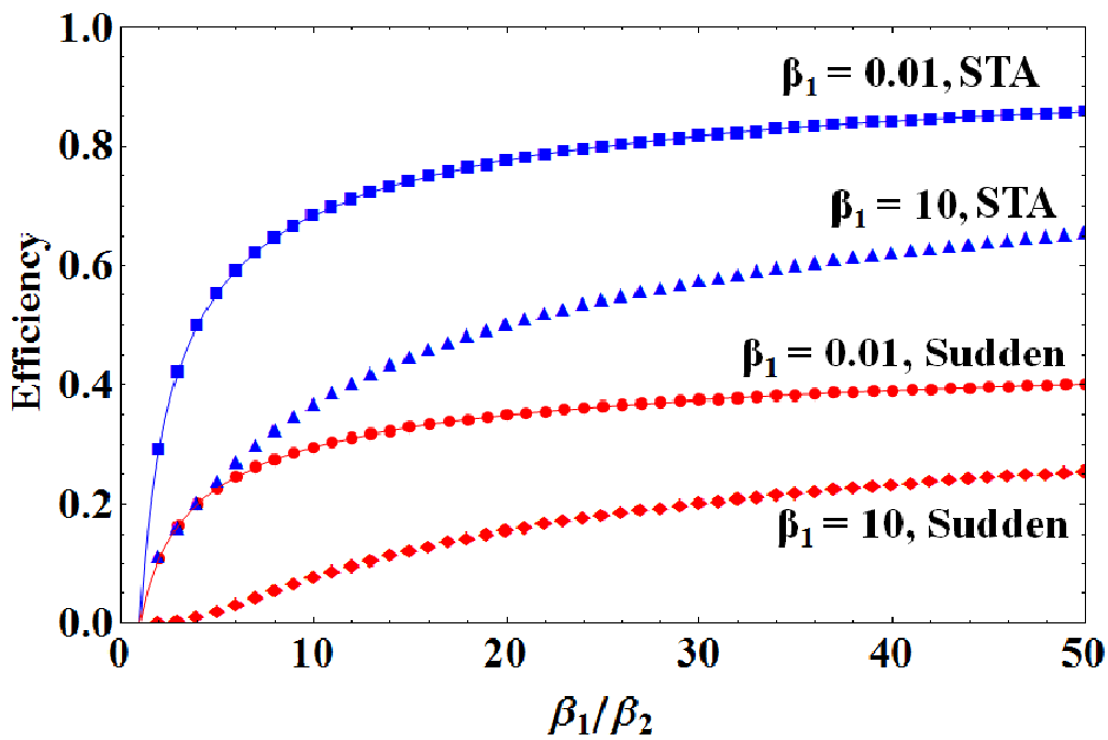
For the heat engine operating in the quantum regime, we consider quantum STA for steps 1 and 3. Though the engine power is enhanced, the expression of quantum work output per cycle remains the same as in Ref. [17]. The efficiencies with optimized are shown in Fig. 4. For a large such as , the obtained efficiency results can be far off from the two classical curves (solid lines) describing and . This case hence represents an engine operating in the deep quantum domain. Interestingly, there the heat engine efficiency associated with STA is still more than twice of that obtained in the sudden change limit. The enhancement factor is even much larger if approaches .
VI Conclusion
Shortcuts to adiabatic processes are shown to have simple classical counterparts. They can substantially suppress work fluctuations in rapid processes. Work values, though classically positive-definite in a protocol, may be still negative in the quantum domain. However, quantum STA may completely suppress the negative work values. STA can also enhance the efficiency and at the same time as well the power of a micro heat engine, in both classical and quantum regimes. Finally, we compare our work with two related and independent studies [11, 12]. Reference [11] studied the use of STA (in a quantum framework) in a heat engine model, via a tailored time-dependence of the frequency of the parametric oscillator setup [5]. Though using a different control scheme, the main conclusion drawn in Ref. [11] echoes with ours in the heat engine application. Reference [12] also studied the classical analog of quantum STA, but using concepts and techniques different from this work.
Appendix A for Quantum Parameteric Oscillator
Here we provide some necessary details regarding the quantum control Hamiltonian for realizing STA. In our main text we consider a quantum parametric oscillator, whose Hamiltonian is given by with a time dependent angular frequency . The calculations for can be found from Ref. [15]. For a self-containing comparison with our classical theory, we first perform a similar calculation here. Obviously
| (30) |
and
| (31) |
Note also that
| (32) |
where , are annihilation and creation operator. The quantum transitionless driving Hamiltonian derived in Ref. [2] is
| (33) | |||||
from which we have
| (34) | |||||
This is just the expression of given in Ref. [15].
Appendix B for Classical Parametric Oscillator
For a classical parametric oscillator , we have [20]
| (35) |
In addition, a type-II generating function relates and through
| (36) |
and
| (37) |
Equation (36) leads to
| (38) |
Therefore
| (39) |
where is arbitrary and we set it to , which then gives
| (40) |
The control Hamiltonian defined in the main text is then given by
| (41) | |||||
As such, one directly has as given in the main text.
Appendix C Work Function in Bare Non-Adiabatic Processes
To compare with the work function in classical STA, we also present analytical results for the work functions in classical (bare) non-adiabatic processes, using a parametric oscillator as a specific system. To that end we first need to specify . In particular, we consider a positive-valued angular frequency
| (42) |
so that at . For brevity we assume , i.e. is increasing during the entire protocol. Then, we have
| (43) | |||||
which clearly indicates that the classical work for a protocol using a monotonically increasing is positive-definite. Interestingly, as seen in the main text, this is not true in the quantum case.
The equation of motion is
| (44) |
There are two linearly independent special solutions and with
| (45) |
Under our specific choice of in Eq. (42) (see also Ref. [28]), and are the basic solutions to Mathieu’s equation [31]:
| (46) |
where and . Then a general solution with initial condition is given by
| (47) |
Once we have the solution , our following derivations will be quite general.
The work done during a time duration is
| (48) | |||||
where , , and
| (49) |
Note that , and defined above are independent of and hence independent of and . Because in Eq. (48) is expressed in a quadratic form, there always exist a two-dimensional orthogonal transformation such that
| (50) |
with
| (51) |
and related to by an orthogonal transformation (such that ). Since the work is known to be positive-definite (under our specific choice of ), must be positive. The initial Gibbs ensemble under inverse temperature then becomes
| (52) |
Finally, the classical work function is
where a change of integration variable ( and with and is used.
References
- [1] M. Demirplak and S. A. Rice, J. Phys. Chem. A 107, 9937 (2003); J. Phys.Chem. B109, 6838 (2005); J. Chem. Phys. 129, 154111 (2008).
- [2] M. V. Berry, J. Phys. A: Math. Theo. 42, 365303 (2009).
- [3] S. Masuda and K. Nakamura, Proc. R. Soc. A 466, 1135 (2009).
- [4] X. Chen, I. Lizuain, A. Ruschhaupt, D. Guéry-Odelin, and J. G. Muga, Phys. Rev. Lett. 105, 123003 (2010).
- [5] X. Chen, A. Ruschhaupt, S. Schmidt, A. del Campo, D. Guéry-Odelin, and J. G. Muga, Phys. Rev. Lett. 104, 063002 (2010).
- [6] S. Choi, R. Onofrio, and B. Sundaram, Phys. Rev. A84, 051601 (R) (2011).
- [7] J. F. Schaff, P. Capuzzi, G. Labeyrie, and P. Vignolo, New J. Phys. 13, 113017 (2011).
- [8] M. G. Bason, M. Viteau, N. Malossi, P. Huillery, E. Arimondo, D. Ciampini, R. Fazio, V. Giovannetti, R. Mannella and O. Morsch, Nature Physics 8, 147 (2012).
- [9] J. F. Zhang, J. .H Shim, I. Niemeyer, T. Taniguchi, T. Teraji, H. Abe, S. Onoda, T. Yamamoto, T. Ohshima, J. Isoya, and D. Suter, Phys. Rev. Lett. 110, 240501 (2013).
- [10] A. del Campo, Phys. Rev. Lett. 111, 100502 (2013).
- [11] A. del Campo, J. Goold, and M. Paternostro, arXiv: 1305.3223.
- [12] C. Jarzynski, Phys. Rev. A88, 040101(R) (2013).
- [13] A. del Campo and M. G. Boshier, Sci. Rep. 2, 648 (2012); A. del Campo, Phys. Rev. A84, 031606(R) (2011).
- [14] Note that the classical integrability condition can be relaxed in quantum systems, see, e.g., [11, 13].
- [15] J. G. Muga, X. Chen, S. Ibáez, I. Lizuain, and A. Ruschhaupt, J. Phys. B 43, 085509 (2010).
- [16] Y. Rezek and R. Kosloff, New J. Phys. 8, 83, (2006).
- [17] O. Abah, J. Ronagel, G. Jacob, S. Deffner, F. Schmidt-Kaler, K. Singer, and E. Lutz, Phys. Rev. Lett. 109, 203006 (2012).
- [18] M. V. Berry, Proc. R. Soc. Lond. A 392, 1802 (1984).
- [19] Some details are in J. W. Deng, Q.-h. Wang, and J. B. Gong, arxiv: 1305.4207.
- [20] H. Goldstein, C. Poole, and J. Safko, Classical Mechanics (Pearson, N. J. , 2002), 3rd ed.
- [21] C. Jarzynski, Phys. Rev. Lett. 78, 2690 (1997).
- [22] C. Jarzynski, C. R. Physique 8, 495 (2007).
- [23] M. Campisi, P. Hänggi and P. Talkner, Rev. Mod. Phys. 83, 771 (2011); ibid, Rev. Mod. Phys. 83, 1653 (E)(2011).
- [24] P. Talkner, E. Lutz, and P. Hänggi, Phys. Rev. E75, 050102 (2007).
- [25] C. Jarzynski, Phys. Rev. E56, 5018 (1997).
- [26] S. Vaikuntanathan and C. Jarzynski, Phys. Rev. Lett. 100, 190601 (2008); J. Chem. Phys.134, 054107 (2011).
- [27] S. Deffner and E. Lutz, Phys. Rev. E77, 021128 (2008).
- [28] S. Deffner, O. Abah, and E. Lutz, Chem. Phys. 375, 200 (2010).
- [29] P. Talkner, M. Morillo, J. Yi, and P. Hänggi, New J. Phys. 15, 095001 (2013).
- [30] F. L. Curzon and B. Ahlborn, Am. J. Phys. 43, 22 (1975).
- [31] NIST Handbook of Mathematical Functions (New York, Cambridge University Press), 2010 (edited by F. W. J. Olver).