Hardcore bosons in a zig-zag optical superlattice
Abstract
We study a system of hard-core bosons at half-filling in a one-dimensional optical superlattice. The bosons are allowed to hop to nearest and next-nearest neighbor sites. We obtain the ground state phase diagram as a function of microscopic parameters using the finite-size density matrix renormalization group (FS-DMRG) method. Depending on the sign of the next-nearest neighbor hopping and the strength of the superlattice potential the system exhibits three different phases, namely the bond-order (BO) solid, the superlattice induced Mott insulator (SLMI) and the superfluid (SF) phase. When the signs of both hopping amplitudes are the same (the “unfrustrated” case), the system undergoes a transition from the SF to the SLMI at a non-zero value of the superlattice potential. On the other hand, when the two amplitudes differ in sign (the “frustrated” case), the SF is unstable to switching on a superlattice potential and also exists only up to a finite value of the next nearest neighbor hopping. This part of the phase diagram is dominated by the BO phase which breaks translation symmetry spontaneously even in the absence of the superlattice potential and can thus be characterized by a bond order parameter. The transition from BO to SLMI appears to be first order.
pacs
03.75.Nt, 05.10.Cc, 05.30.Jp, 73.43NqI Introduction
Ultracold atoms provide a unique opportunity to investigate a wide range of phenomena, especially in low dimensions where quantum fluctuations play a dominant role [1]. Because of the exquisite control and precision possible experimentally, they offer nearly perfect realizations of various model condensed matter systems. The seminal paper by Jaksch et al [2] which had predicted the quantum phase transition from Mott insulator to superfluid phase in the Bose-Hubbard model, paved the way for the first experimental observation of this transition in an optical lattice by Greiner et al [3]. Current experimental techniques have successfully created various lattice geometries using proper arrangements of laser beams, such as optical superlattices [4, 5], triangular [6] and Kagome lattices [7]. Such a diverse class of lattice systems gives us the opportunity to study a variety of models which might also be geometrically frustrated. The interatomic interactions can be controlled to a high degree of accuracy with the help of Feshbach resonances [8]. Recent developments in shaking techniques have enabled experimentalists to modify the value and sign of the intersite hopping [9, 10] thus opening up possibilities to investigate frustrated systems of bosonic lattice gases [11].

Earlier works on ultracold bosons in optical superlattice have shown the existence of phases with density wave-like configurations [12, 13, 14, 15, 16, 17]. Later studies of soft-core bosons in optical superlattices [18, 19] termed these phases as superlattice induced Mott insulator(SLMI) phases. Recent studies on models dealing with the interplay between frustration imposed by geometry and interactions have revealed rich physics with a variety of novel phases being exhibited [20, 21, 22, 23].
In this paper, we analyze a system of hardcore bosons in a superlattice with nearest and next-nearest neighbor hoppings. The superlattice potential creates an energy offset in alternate sites. This model is equivalent to a zig-zag superlattice as shown in Fig. 1. The nearest and the next-nearest neighbor hoppings are equivalent to the hoppings between the legs and within the legs of the zig-zag lattice respectively. The energy offset can be introduced by applying a constant electric field in the y-direction as shown in Fig. 1. In such a situation the system can be described by the Hamiltonian given by
| (1) | |||||
where and are creation and annihilation operators for hard core bosons at site , and is the boson number operator at site . Here and are the hopping amplitudes for tunneling to a neighboring site and a next-nearest neighbor site respectively and is the superlattice potential. In the present work, we have considered a two-period superlattice, with for odd and zero for even . We assume that the values of from even to even sites and from odd to odd sites are equal in magnitude. In other words the hopping amplitudes along the legs of the zig-zag lattice are the same. A similar assumption has been made in an earlier work on square ladder [15] and also in a recent experiment in a sqaure lattice [5]. We study the system for a wide range of and and we fix the energy scale in the units of by taking the value of .

When the above model can be mapped onto a non-interacting model of spinless fermions. Using the Jordan-Wigner transformation [24]
| (2) |
Eq. (1) can be mapped to
| (3) |
where and are the creation and annihilation operators for the spinless fermions and is the fermion number operator. The single particle eigenstates of the Hamiltonian given by Eq. (3) can be obtained exactly. There are two bands arising from the fact that the translational symmetry of the lattice has been broken by the superlattice potential. The energy spectra of the two bands are given by
| (4) |
where is the lattice spacing and , the crystal momentum that runs from to . A plot of these spectra is shown in Fig. 2. From this figure and Eq. (4), it can be seen that there is a gap equal to at half filling. Turning on augments the effect of if they have the same sign yielding a superfluid as we show below. For the opposite sign of the system is frustrated and we find that this frustration coupled with the superlattice potential prevents superfluidity from occurring. For either sign of , the model can no longer be mapped onto one of non-interacting spinless fermions and thus we have to take recourse to numerics to study it. We do this via a state-of-the art density matrix renormalization group (DMRG) method [25].
The remaining part of the paper is organized as follows. In Section II, we outline the method of calculation we have used, followed by a presentation of results in Section III and a summary of our conclusions in section IV.
II Method of calculation
We study the ground state properties of the model described by Eq. (1) using the finite-size DMRG method with open boundary conditions [26, 27] which is best suited to (quasi-)one-dimensional problems [27]. For our calculations we study system sizes up to 300 sites and retain density matrix eigenstates with the weight of the discarded states in the density matrix being less than .
In order to obtain the ground state phase diagram we calculate several physical quantities of interest. Some of these quantities have been calculated by us using the DMRG method to study related models [23, 28]. To separate out the gapped and gapless phases we calculate the single particle excitation gap given by
| (5) |
In Eq. (5), is the ground-state energy of a system with sites and bosons. To identify the BO phase we compute the bond order parameter given by
| (6) |
where is the bond energy. The presence of the SLMI phase can be determined through a calculation of the structure factor obtained by taking the Fourier transform of the density-density correlation function
| (7) |
We also calculate the momentum distribution function given by
| (8) |
Before discussing the results obtained from our FS-DMRG calculation we mention that we have verified that our numerical method gives us very accurate results in the analytically tractable case . We compute the single particle excitation gap using Eq. (5) for this case, which from the analysis of the previous section is equal to . Our numerics give us a gap which is within percent for various values of . We thus believe that our FS-DMRG calculation yields very accurate results even for .
III Results

We now discuss the results of the present work. Before we give the results of our numerical calculations in detail, we present arguments for the general structure of the phase diagram. As discussed in section I, when , the system has a gap for any finite value of . The presence of the gap would make the state robust to perturbations due to , till they get to be roughly of the order of the gap. The SLMI phase is the adiabatic continuation of the gapped phase for . The gap at increases with increasing . As a result, the extent of the SLMI phase along the axis will be larger as increases. This can indeed be seen in the phase diagram obtained from our numerical calculations shown in Fig. 3, where we have set the energy scale by .
We now consider the phases that arise at large values of after the SLMI phase has disappeared. We note that when , our model as described in Eq. (1) is same as hardcore bosons hopping on a triangular ladder. For , we have determined from DMRG calculations that the ground state is always a superfluid and we find that this state is not immediately destroyed by a non-zero value of . There is thus a phase boundary between the SLMI and SF as shown in Fig. 3 in the plane. For and , the system is “frustrated” and it is known that the superfluid does not persist up to arbitrarily large values of [23]. The superfluid persists up to after which a gapped bond ordered (BO) phase forms through a Berezinski-Kosterlitz-Thouless (BKT) type transition. A physical picture of the BO phase can be obtained by studying the model at the exactly solvable point , where it can be mapped onto an version of the spin 1/2 Majumdar-Ghosh spin chain [29]. The BO phase is a valence bond solid, where the valence bonds are of the type for adjacent sites and . Note, that this state spontaneously breaks translational symmetry even for . Since the BO phase is gapped, we expect it to be stable up to a critical value of after which the SLMI phase emerges. This is indeed the case as can be seen from Fig. 3. The SF phase that exists below , however, appears to be unstable to the introduction of in contrast to the SF phase for . It should be noted that though both the SLMI and the BO phases are gapped and not translationally invariant, they are fundamentally different in that the BO phase has a non-zero BO order parameter given by Eq. (6), which is zero for the SLMI phase. All three phases have a non-zero structure factor given by Eq. (7) when since translational symmetry is being broken by hand. However, as we will show there is a kink in the structure factor as a function of at the boundary between the BO and SLMI.
III.1 Positive case
As argued above, we expect a transition between the SLMI and SF phases for . Since this transition is from a gapped to gapless phase, it is determined numerically by calculating the single particle

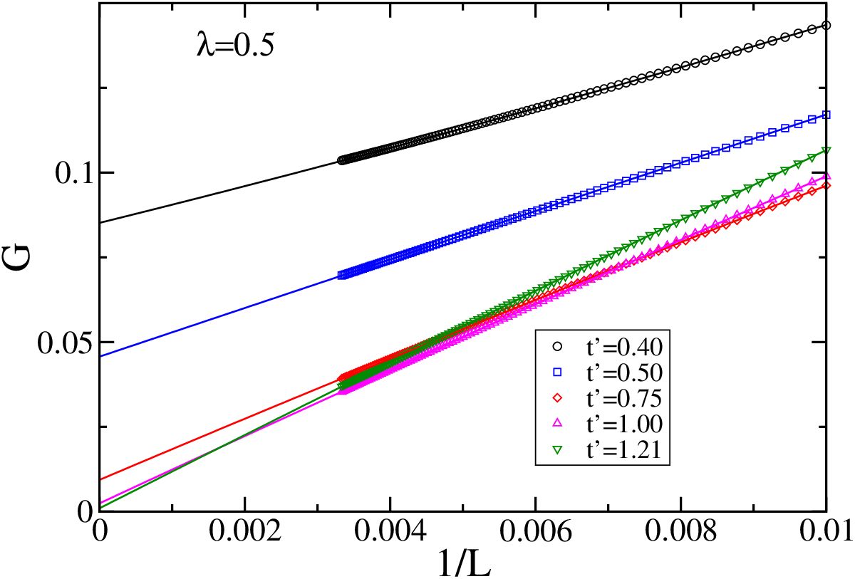
excitation gap as defined in Eq. (5). We perform a finite size scaling of the gap by fitting a quadratic polynomial in and extrapolating it to to get the thermodynamic limit values of . For the fitting we consider fairly large system sizes i.e. from to . The extrapolated values of as a function of for are shown in Fig. 4 which clearly shows a transition from a gapped to gapless phase. The gap appears to close slowly as the value of approaches the critical value at . In Fig. 5 we show the finite size scaling of the gap for different values of . It can be seen that the fitting functions gradually go to zero as the transition point approaches. We estimate the critical point by noting that the extrapolated gap appears to stabilize to a value that is less than . Since, we expect the gap to approach to zero in the true thermodynamic limit in the SF phase, we obtain the phase boundary by using the criterion that for less than the system is gapless.
III.2 Negative case
To determine the BO phase, we calculate the order parameter and plot it as a function of for different values of . This is done for in Fig. 6.

It can be clearly seen that for small values of , there is an exponential decay in (Figs. 6(a)-(d)). However, in Fig. 6(e), we observe the emergence of long-range bond oscillations. In Figs. 6(e) and (f), there are distinct oscillations throughout the lattice. This indicates the presence of the BO phase at higher negative values of . In order to locate the transition to the BO phase we compute the bond-order parameter defined in Eq. (6).

We plot the thermodynamic values of the obtained from a third order polynomial extrapolation, as shown in Fig. 7. The BO phase is expected to have a finite whereas it will be zero in the SLMI phase. As can be clearly seen from the figure, a discrete jump in its value is noticed, which is further supported by a sharp peak in the first derivative as shown in the inset. This clearly signifies a phase transition to the BO phase from the SLMI phase. The transition is located by taking the derivative maximum of the given by , as shown in the inset of Fig. 7.
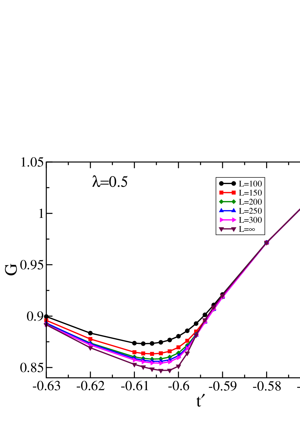
The bond order parameter calculation to locate the SLMI-BO transition critical point is complemented by the scaling of the single particle excitation gap . In Fig. 8 we plot as a function of for different lengths and for obtained by extrapolation. It can be seen that the system is always gapped along the axis. The gap decreases as the critical point approaches and remains finite and then increases again. The minimum shifts towards the actual critical point for larger lengths. Extrapolating to the thermodynamic limit we find the minimum to occur at the critical point as obtained from the scaling. Note, however, that the gap does not go to zero at the transition indicating a first order transition consistent with the jump of the BO order parameter.

The imposition of the superlattice potential will cause a density modulation of the type […1 0 1 0 …] in all the three phases. The structure factor, , as defined in Eq. (7) will show finite peaks at , whose heights are large in the SLMI phase and smaller in the BO and the SF phases. The thermodynamic value of is plotted for in Fig. 9. In the BO phase, is small and increases steadily with decreasing . At the transition point between BO and SLMI, it has a kink and then increases gradually as the value of approaches . A similar plot for a smaller value of is shown in Fig. 10 showing a similar peak in the negative region at the transition point. In the positive region, both Fig. 9 and 10 show a gradual decrease in the value of as the system undergoes a transition from SLMI to SF phase.

We have also obtained the momentum distribution since it can, in principle, be observed experimentally through time-of-flight images and plotted it in Fig. 11. In BO phase, two peaks appear, which shift away from . But as the system enters the SLMI phase, it shows a broad peak at around . (Figs. 11(a) and (b)). The two peak structure in the BO phase is obtained even for and has been investigated earlier [23]. For positive region, the population of atoms in the state is small, as indicated in Fig. 11(c) but as the system enters the SF region, the starts filling up resulting in a large peak as shown in Fig. 11(d).

IV Conclusions
We have obtained the phase diagram of a model of hard-core bosons in a 1D lattice with nearest neighbor hopping ( set to the value of ) and next-nearest neighbor hopping () in the presence of a superlattice potential (). We find that the phases obtained depend on the sign of . For , there are two phases, a gapped superlattice induced Mott insulator (SLMI) and a gapless superfluid (SF). The superfluid is stable to switching on the superlattice potential and a finite value of is required to drive the SF into the SLMI. On the other hand for , we obtain in addition to the SF and SLMI, a gapped bond ordered (BO) phase. The SF phase for is unstable to switching on a superlattice potential and thus exists only for up to a finite value of . The BO phase exists even when and thus spontaneously breaks lattice translational symmetry and can be characterized by a bond order parameter. The transition from the BO to the SLMI phase appears to be first order.
V Acknowledgments
The computations reported in this work were performed using the Intel HPC (Hydra) Cluster at IIA, Bangalore, India. We thank Abhishek Dhar for many useful discussions. R.V.P. acknowledges financial support from U.G.C. India. S. M. thanks the Department of Science and Technology of the Government of India for support.
References
- [1] M. A. Cazalilla, R. Citro, T. Giamarchi, E. Orignac, M. Rigol, Rev. Mod. Phys. 83, 1405 (2011).
- [2] D. Jaksch, C. Bruder, J. I. Cirac, C. W. Gardiner, and P. Zoller, Phys. Rev. Lett. 81, 3108 (1998).
- [3] M. Greiner, O. Mandel, T. Esslinger, T. W. Hansch, and I. Bloch, Nature (London) 415, 39 (2002).
- [4] P. Cheinet, S. Trotzky, M. Feld, U. Schnorrberger, M. Moreno-Cardoner, S. Foelling, I. Bloch, Phys. Rev. Lett. 101, 090404 (2008).
- [5] M. Aidelsburger, M. Atala, S. Nascimbène, S. Trotzky, Y.-A. Chen, I. Bloch, Phys. Rev. Lett, 107, 255301 (2011); Applied Physics B, Volume 113, Issue 1, pp 1-11 (2013)
- [6] C. Becker et al New J. of Physics, 12, 065025 (2010).
- [7] G.-B. Jo, J. Guzman, C. K. Thomas, P. Hosur, A. Vishwanath, and D. M. Stamper-Kurn Phys. Rev. Lett. 108, 045305 (2012).
- [8] C. Chin et al Rev. Mod. Phys. 82, 1225 (2010).
- [9] A. Eckardt, C. Weiss, and M. Holthaus, Phys. Rev. Lett. 95, 260404 (2005).
- [10] A. Zenesini, H. Lignier, D. Ciampini, O. Morsch, and E. Arimondo, Phys. Rev. Lett. 102, 100403 (2009).
- [11] J. Struck et al Science 333, 996 (2011).
- [12] Robert Roth, Keith Burnett, Phys. Rev. A 68, 023604 (2003).
- [13] V. G. Rousseau, D. P. Arovas, M. Rigol, F. Hèbert, G. G. Batrouni, R. T. Scalettar, Phys. Rev. B 73, 174516 (2006).
- [14] M. Rigol, A. Muramatsu, M. Olshanii, Phys. Rev. A 74, 053616 (2006).
- [15] I. Danshita, J. E. Williams, C. A. R. Sá de Melo, C. W. Clark, Phys. Rev. A 76, 043606 (2007).
- [16] Guo Huai-Ming and Liang Ying, Commun. Theor. Phys. (Beijing, China) 50, 1142 (2008).
- [17] Bo-Lun Chen, Su-Peng Kou, Yunbo Zhang, Shu Chen, Phys. Rev. A 81, 053608 (2010).
- [18] A. Dhar, T. Mishra, R. V. Pai and B. P. Das, Phys. Rev. A 83, 053621 (2011).
- [19] A. Dhar, M. Singh, R. V. Pai and B. P. Das, Phys. Rev. A 84, 033631 (2011).
- [20] A. Dhar, M. Maji, T. Mishra, R. V. Pai, S. Mukerjee and A. Paramekanti, Phys. Rev. A (R) 85, 041602 (2012).
- [21] A. Dhar, T. Mishra, M. Maji, R. V. Pai, S. Mukerjee and A. Paramekanti, Phys. Rev. B 87, 174501 (2013)
- [22] S. Greschner, L. Santos and T. Vekua, Phys. Rev. A 87, 033609 (2013).
- [23] T. Mishra, R. V. Pai, S. Mukerjee and A. Paramekanti, Phys. Rev. B 87, 174504 (2013).
- [24] P. Jordan, E. Wigner, Z. Phys. 47, 631 (1928).
- [25] S. R. White, Phys. Rev. B 48, 10345 (1993).
- [26] S. R. White, Phys. Rev. Lett. 69, 2863 (1992).
- [27] U. Schollwöck, Rev. Mod. Phys. 77, 259 (2005).
- [28] T. Mishra, J. Carrasquilla, and M. Rigol Phys. Rev. B bf 84, 115135 (2011)
- [29] C. K. Majumdar, D. K. Ghosh, J. Math. Phys. 10, 1388 (1969).