Stabilizing the Semilocal String with a Dilatonic Coupling
Abstract
We demonstrate that the stability of the semilocal vortex can be significantly improved by the presence of a dilatonic coupling of the form with where is the scale of symmetry breaking that gives rise to the vortex. For we obtain the usual embedded (semilocal) Nielsen-Olesen vortex. We find the stability region of the parameter ( and are the masses of the scalar and gauge fields respectively). We show that the stability region of is where (as expected) and is an increasing function of . This result may have significant implications for the stability of the electroweak vortex in the presence of a dilatonic coupling (dilatonic electroweak vortex).
The Nielsen-Olesen (NO) vortex [1, 2] is a topologically stable static solution of the Abelian-Higgs model. The Lagrangian density of this model is of the form
| (1) |
where is a complex scalar field, , and .
The NO vortex ansatz is of the form11 1 In the numerical analysis of this study we have set the winding number .
| (2) | |||||
| (3) |
Variation of the Lagrangian (1) leads to the field equations for and as
| (4) | |||
| (5) |
where and we have implemented the following rescaling:
| (6) | |||||
| (7) |
The NO boundary conditions to be imposed on (4) and (5) are , and . Clearly, the NO solution for , depends on a single parameter which is the squared ratio of the scalar field mass over the gauge field mass .
The energy density of the NO vortex is of the form
| (8) |
The NO vortex solution can also be embedded in generalizations of the Abelian-Higgs model. For example the semilocal Lagrangian [3]
| (9) |
is obtained by promoting the symmetry of the Abeian-Higgs model to an symmetry. This is achieved by replacing the complex scalr by a complex doublet
| (10) |
The embedded NO vortex ansatz (semilocal vortex) is of the form
| (11) |
while for the gauge field eq. (3) remains unchanged. By varying the semilocal Lagrangian it is easy to show that the field equations obeyed by and (or ) are identical to the NO equations (4) and (5). Thus the NO vortex solution is embedded in the generalized semilocal Lagrangian. However, due to the topology of the semilocal vacuum, the stability of the embedded vortex is not topological. It is only dynamical and is valid for a finite range of the parameter . It may be shown [4, 5, 6, 7] that this range of stability is .
The NO vortex can be embedded in several other generalizations of the Abelian-Higgs model which involve broken U(1) symmetries. For example it can be embedded in the bosonic sector of standard Glashow-Salam-Weinberg (GSW) electroweak model [8] with symmetry. One type of such embedded vortices is also known as the electroweak -vortex[9, 10, 11]. There is a parameter region of dynamical stability of the electroweak -vortex. It is determined by two parameters: the squared ratio of the Higgs mass over the mass () and the Weinberg angle [11]. Thus, the stability range of the embedded electroweak -vortex is of the form . For the bosonic sector of the GSW Lagrangian reduces to the semilocal Lagrangian and therefore . For we have and therefore the stability range decreases. The experimental values and are outside of the stability region [11].
There has been a wide range of studies aiming at constructing models where the stability of the semilocal and/or electroweak vortex is improved. These studies have attempted to improve the stability using thermal effects [12], extra scalar fields [13, 14], external magnetic fields [15], fermions [17, 16] or spinning scalar field in a charged background [18]. Most of these studies have either lead to models where the vortex stability is worse than the usual semilocal Lagrangian or to particularly contrived models requiring external backgrounds. Even for the classical stability region of semilocal and electroweak strings, there are instabilities at the quantum level [19].
In this study we attempt to increase the stability region of the semilocal vortex by considering a simple and generic generalization of the Abelian-Higgs model Lagrangian: the dilatonic Abelian-Higgs model defined to be of the form
| (12) |
where is a dilatonic coupling that allows for dynamics of the effective gauge coupling . In the limit () we obtain the usual Abelian-Higgs model with the NO vortex solution.

Considering now the NO ansatz in the dilatonic Abelian-Higgs model we obtain the rescaled field equations for the dilatonic gauge vortex
| (13) | |||||
| (14) |
where as usual . The corresponding energy density is of the form
| (15) |
Using the NO boundary conditions, it is straightforward to obtain the dilatonic vortex solution of equations (13), (14) for various values of the parameters and (Fig 1). A simple mathematica code for the derivation of this solution, based on the minimization of the energy density (15), is provided in the Appendix.
In order to investigate the stability of the embedded dilatonic vortex we generalize the dilatonic Abelian-Higgs Lagrangian to a dilatonic semilocal Lagrangian with symmetry.
| (16) |
We then consider the perturbed fields and as
| (17) |
| (18) |
The energy perturbations due to and decouple and can only lead to increase of the embedded dilatonic vortex energy. The corresponding energy perturbation is identical to the energy perturbation of the topologically stable NO vortex and therefore it is positive definite. Thus the stability of the dilatonic embedded vortex is determined by the energy perturbation due to . The energy of the perturbed vortex is of the form
| (19) | |||||
where we have included only perturbations due to and is the unperturbed energy of the embedded dilatonic vortex. The energy perturbation due to may be written in the form
| (20) |
where is a Schrodinger-like Hermitian operator of the form
| (21) |
and we have only kept terms up to second order in . The Schrodinger potential corresponding to is
| (22) |
For values of the parameters and for which has no negative eigenvalues we have and therefore no instability develops. In order to determine if has negative eigenvalues we may solve with boundary conditions , and check if the solution crosses the line and goes to asymptotically. If it does then it is easy to show that there must exist at least one bound state (negative eigenvalue).

The parameter region in the space where has no negative eigenvalues is shown in Fig. 2 (sector I). In order to construct this plot, for each value of we find a stability region . As expected . Interestingly and the stability region increases as we increase . The improvement of stability is due to the fact that the effective Schrodinger potential (22) corresponding to the operator becomes shallower as we increase (Fig. 3). Thus becomes less receptive to negative eigenvalues.The new repulsive term in the Schrodinger potential (22) (proportional to ) originates from the dilatonic term in the Lagrangian (16). This term favors energetically a lower value for the field at the origin and therefore it makes the perturbation more costly energetically at . This leads to improved stability for the dilatonic embedded gauge vortex.
We have also investigated the dilatonic embedded global vortex in the presence of an external magnetic field. This solution is obtained by replacing the covariant derivatives in the Lagrangian (12) by regular ones. In the absence of a dilatonic coupling this vortex is unstable and there is no free parameter in the Lagrangian. However, in the presence of a dilatonic coupling and a gaussian external magnetic field we have shown that the embedded global vortex gets stabilized in the region where the magnetic field is present. These results will be presented elsewhere.

The existence of dilatonic gauge and global vortices may also have implications as a new class of models predicting spatial variation of the fine structure constant on cosmological scales. Such models have been discussed in Ref. [22, 23, 24, 25, 26] and are motivated from recent quasar absorption spectra observations that may hint towards possible spatial variation of on cosmological Hubble scales [27].
The dilatonic semilocal model is perhaps the simplest generalization of the semilocal model that can lead to dramatic improvement of the semilocal vortex stability. The existence of such a dilatonic coupling in the realistic GSW model is therefore also expected to lead to improvement of the stability of the -string [20, 21] and perhaps create a stability region for the -string (an alternative embedding of the NO vortex in the GSW model) [20]. The analysis of the stability of the dilatonic electroweak vortices constitutes and interesting extension of the present study.
We thank Tanmay Vachaspati for useful comments and John Rizos for his help on some numerical aspects of this work. This research has been co-financed by the European Union (European Social Fund - ESF) and Greek national funds through the Operational Program Education and Lifelong Learning of the National Strategic Reference Framework (NSRF) - Research Funding Program: ARISTEIA. Investing in the society of knowledge through the European Social Fund.
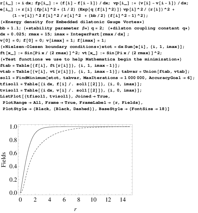
I Appendix
In Fig. 4 we show the Mathematica code used to find numerically the dilatonic vortex solutions by minimization of the energy functional (15). The algorithm is particularly simple and has a wide range of applications including the numerical derivation of the NO vortex solution. Note that due to stiffness of the ODE system (13)-(14), Mathematica is unable to solve it using the NDSolve routine. A similar code can be used to investigate the stability of the embedded dilatonic vortex by minimizing the energy functional (19) with respect to the three functions , and . For parameter values leading to a non-zero at the defect core we have instability. Even though this approach is more involved and subject to some numerical uncertainties, in most cases it leads to consistent results with the more accurate and simple perturbative method based on finding if the operator has negative eigenvalues.
References
- [1] H. B. Nielsen and P. Olesen, Nucl. Phys. B61 (1973) 45.
- [2] L. Perivolaropoulos, Phys. Rev. D48 (1993) 5961.
- [3] T. Vachaspati and A. Achúcarro, Phys. Rev. D44, 3067 (1991).
- [4] M. Hindmarsh, Phys. Rev. Lett. 68 (1992) 1263.
- [5] M. Hindmarsh, Nucl. Phys. B392 (1993) 461.
- [6] A. Achúcarro, K. Kuijken, L. Perivolaropoulos and T. Vachaspati, Nucl. Phys. B388 (1992) 435.
- [7] A. Achúcarro, J. Borrill and A. R. Liddle, Phys. Rev. Lett. 82 (1999) 3742.
- [8] G. Glashow, Nucl. Phys 22 (1961) 579; S. Weinberg, Phys. Rev. Lett. 19 (1967) 1264; A. Salam, in “Elementary particle physics” (Nobel Symp. no. 8), ed. N. Svartholm, Almqvist and Wilsell, Stockholm 1968.
- [9] Y. Nambu, Nucl. Phys. B130 (1977) 505.
- [10] T. Vachaspati, Nucl. Phys. B 397, 648 (1993).
- [11] M. James, L. Perivolaropoulos and T. Vachaspati, Phys. Rev. D46 (1992) R5232; Nucl. Phys. B395 (1993) 534.
- [12] R. Holman, S. Hsu, T. Vachaspati and R. Watkins, Phys. Rev. D46 (1992) 5352.
- [13] M. A. Earnshaw and M. James, Phys. Rev. D48 (1993) 5818.
- [14] T. Vachaspati and R. Watkins, Phys. Lett. B318 (1993) 163.
- [15] J. Garriga and X. Montes, Phys. Rev. Lett. 75 (1995) 2268.
- [16] S. Naculich, Phys. Rev. Lett. 75 (1995) 998.
- [17] M. A. Earnshaw and W. B. Perkins, Phys. Lett. B328 (1994) 337.
- [18] L. Perivolaropoulos, Phys. Rev. D50 (1994) 962.
- [19] J. Preskill and A. Vilenkin, Phys. Rev. D47 (1992) 4218.
- [20] A. Achucarro and T. Vachaspati, Phys. Rept. 327, 347 (2000) [Phys. Rept. 327, 427 (2000)] [hep-ph/9904229].
- [21] P. Goddard and D. Olive, Rep. Prog. Phys. 41 (1978) 1357-1437; T. W. B. Kibble, Phys. Rep. 67 (1980) 183; A. Vilenkin Phys. Rep. 121 (1985) 1; J. Preskill, “Vortices and Monopoles”, lectures presented at the 1985 Les Houches Summer School, Les Houches France; A. Vilenkin and E. P. S. Shellard, “Cosmic Strings and Other Topological Defects”, Cambridge University Press, Cambridge (1994); R. Brandenberger, Int. J. Mod. Phys. A9 (1994) 2117; M. Hindmarsh and T. W. B. Kibble, Rep. Prog. Phys. 58 (1995) 477.
- [22] A. Mariano and L. Perivolaropoulos, Phys. Rev. D 86, 083517 (2012) [arXiv:1206.4055 [astro-ph.CO]];
- [23] A. Mariano and L. Perivolaropoulos, Phys. Rev. D 87, 043511 (2013) [arXiv:1211.5915 [astro-ph.CO]].
- [24] J. C. Bueno Sanchez and L. Perivolaropoulos, Phys. Rev. D 84, 123516 (2011) [arXiv:1110.2587 [astro-ph.CO]].
- [25] K. A. Olive, M. Peloso and A. J. Peterson, Phys. Rev. D 86, 043501 (2012) [arXiv:1204.4391 [astro-ph.CO]].
- [26] K. A. Olive, M. Peloso and J. -P. Uzan, Phys. Rev. D 83, 043509 (2011) [arXiv:1011.1504 [astro-ph.CO]].
- [27] J. A. King, J. K. Webb, M. T. Murphy, V. V. Flambaum, R. F. Carswell, M. B. Bainbridge, M. R. Wilczynska and F. E. Koch, MNRAS 422, 3370 (2012) arXiv:1202.4758 [astro-ph.CO].