Steady state of dust distributions in disk vortices:
Observational predictions and applications to transitional disksNote: Draft version
Abstract
The Atacama Large Millimeter Array (ALMA) has been returning images of transitional disks in which large asymmetries are seen in the distribution of mm-sized dust in the outer disk. The explanation in vogue borrows from the vortex literature by suggesting that these asymmetries are the result of dust trapping in giant vortices, excited via Rossby wave instability (RWI) at planetary gap edges. Due to the drag force, dust trapped in vortices will accumulate in the center, and diffusion is needed to maintain a steady state over the lifetime of the disk. While previous work derived semi-analytical models of the process, in this paper we provide analytical steady-state solutions. Exact solutions exist for certain vortex models. The solution is determined by the vortex rotation profile, the gas scale height, the vortex aspect ratio, and the ratio of dust diffusion to gas-dust friction. In principle, all these quantities can be derived from observations, which would give validation of the model, also giving constrains on the strength of the turbulence inside the vortex core. Based on our solution, we derive quantities such as the gas-dust contrast, the trapped dust mass, and the dust contrast at the same orbital location. We apply our model to the recently imaged Oph IRS 48 system, finding values within the range of the observational uncertainties.
I. Introduction
Transitional disks are a class of circumstellar disks that lack a significant near-infrared (1-5m) excess, while showing steep slopes in mid-infrared (5-20m) and far-infrared (20m) excesses typical of classical T-Tauri disks [105, 104, 32, 113, 11, 13, 80, 102, 24, 26]. This “opacity hole” implies absence of optically thick warm dust in the inner disk, with a dust wall generating the mid-IR emission, followed by cold dust in the outer disk. This, together with their age (in the 1-10 Myr range, see e.g. Currie 25 for a review) provide strong evidence that these are objects caught in the evolutionary stage between gas-rich primordial and gas-poor debris disks, hence the name.
Explanations for the opacity hole generally fall in four distinct categories. These are, namely, grain growth and dust settling [8, 28, 119, 7], photoevaporation [2, 19, 90, 85], dynamical interaction with close stellar or substellar companions [40], and planet formation via dust locking [101, 70, 35, 115, 44] and gap carving [87, 54, 55, 10, 86, 96, 82, 3]. Analyses of individual disks [12, 13, 31] tend to favor one process over another, and even census studies of statistically significant samples of disks find one process to be dominant [82, 19]. These seemingly conflicting results in fact illustrate the heterogeneity of transitional disks, where a combination of all suggested processes are needed to explain the rich diversity observed [20, 81, 77, 100, 21].
Recently, high angular resolution imaging of the outer regions of transitional disks have become available, showing a myriad of puzzling asymmetries that beg for explanation. These come in the shape of spiral arms [93, 23, 79, 107], elliptical dust walls [42], and non-axisymmetric dust clouds [84, 9, 14]. In particular, giant horseshoe-shaped dust distributions are seen in images obtained with the Combined Array for Research in Millimeter-wave Astronomy (CARMA, Isella et al. 41) and with the Atacama Large Millimeter Array (ALMA, Casassus et al. 15, van der Marel et al. 71). The planet interpretation is particularly attractive for explaining these asymmetries, since they generally match the range of structures predicted by hydrodynamical models of planet-disk interaction.
A deep gap is one of these expected structures, as the planet tides expel material from the vicinity of its orbit [87, 54, 55, 83, 72, 86, 96, 111, 49, 68, 118, 50, 51]. The gas gap walls constitute steep pressure gradients, that, by modifying the rotational profile locally, are prone to excite what has been called Rossby wave instability [38, 109, 88, 89, 37, 63, RWI,]. The RWI is an “edge mode” instability akin to Kelvin-Helmholtz, that converts the extra shear into vorticity. The large-scale vortices that result are well-known in the planet formation literature.
Barge & Sommeria [5], Adams & Watkins [1], and Tanga et al. [108] independently proposed, in the context of primordial disks, that vortices could speed up planet formation by trapping solids of cm to m size. The dynamics of this trapping was developed in a detailed work by Chavanis [17], setting much of the analytical foundations of the field. Godon & Livio [33], Godon & Livio [34] and Johansen et al. [43] simulated vortices numerically, finding fast trapping of particles but also quick dissipation due to (Laplacian) viscosity. These studies, however, did not consider the question of how to form disk vortices in first place, a question tackled by [112]. These authors show that a sharp viscosity gradient in the disk leads to a pile-up of matter, that in turn goes unstable to the RWI. Because the magnetorotational instability [4, MRI,] leads to a significant turbulent viscosity, [112] suggest that this mechanism could be at work in the transition between the MRI-active and dead zones. The accumulation of dust in these self-sustained RWI vortices was subsequently studied by Inaba & Barge [39], albeit in the fluid approach, that limited the dust size they could use. Planetary gap edges were seen to excite vortices in many simulations in the code-comparison study of de Val-Borro et al. [111], an effect later explained [110] in terms of the RWI as well.
These efforts culminated into a coherent picture of vortex-assisted planet formation in dead zone vortices by Lyra et al. [69], Lyra et al. [68] and in gap edge vortices by Lyra et al. [67]. These works solved for the nonlinear compressible hydrodynamics and the aerodynamics of interacting particles, demonstrating the gravitational collapse of the trapped solids, albeit in two dimensions. The RWI was subsequently studied in barotropic 3D models by Méheut et al. [73], Méheut et al. [74], Méheut et al. [75], finding interesting meridional circulation patterns; in self-gravitating disks with application to planet migration in 2D [56, 57, 58] and 3D [60], who find weakening and eventual suppression of the RWI with increasing disk mass; in MHD by Lyra & Mac Low [65], bringing realism to the dead-zone scenario; and by Lin [59], Lin [61], who generalized the linear RWI to 3D polytropic and non-barotropic disks, respectively.
Part of these results have been applied to the field of transitional disks. The particle size that is preferentially trapped is set by the friction time, , which is a function of the gas density and particle radius. A suitable nondimensionalization for the friction time is the Stokes number, , where is the Keplerian frequency. Dust that is too well-coupled to the gas () does not suffer friction, and bodies that are too large () have too much inertia to be moved by the gas: the preferential size for trapping is St=1 (see e.g. Youdin & Goodman 114, Youdin 116). While in the dense, fast rotating, inner regions of primordial disks, the preferentially trapped particle size corresponds to meter-size, in the thin, slowly rotating, outer regions of transitional disks, the size corresponding to St=1 drops by about three orders of magnitude [8, 95]. The resulting trapping of sub-mm and mm-size dust may not lead to the critical densities necessary to form planets, but they may well explain the puzzling observed lopsided asymmetries. While the motivation and particle sizes are different, the relevant physics is scale-free, and thus identical as long as gravity is not involved.
This property was invoked by Regály et al. [98] to suggest that the sub-mm observations of Brown et al. [9] could be the result of dust trapping in Rossby vortices. If indeed that is the case, then, as the drag force drives dust toward the vortex center, diffusion is needed to maintain a steady state over the lifetime of the disk [48, 17]. Birnstiel et al. [6] presented a semi-analytical model that solves for the azimuthal dust distribution while using fits from numerical simulations [94] to constrain the radial morphology. In this work we present a fully analytical model for the steady state distribution of dust trapped in vortices, accurate to first order in Stokes number, and general in space. In Sect. II we derive the advective-diffusive equation, and in Sect. III the appropriate coordinate transformation. In Sect. IV we solve the equation for the “axisymmetric” case in that coordinate system, and in Sect. V we generalize it for non-axisymmetry. In Sect. VI we derive observational predictions, and apply the model to the Oph IRS 48 system.
II. Dust steady state
Considering the dust is of small sizes, we can treat it as a fluid. The dust should then follow the continuity equation
| (1) |
where is the dust density, is the dust velocity, and is the diffusion flux. We take it to be
| (2) |
as in the contaminant equation [78, 22, 18], where is the diffusion coefficient (the diffusion is due to elliptical turbulence in the vortex core and in general will be different than the turbulent viscosity in the disk), and is the gas density. We assume that is constant. A list of the mathematical symbols used in this work, together with their definitions, is provided in Table 1.
To derive the velocities, instead of solving the momentum equations for the dust, we make use of the relative velocity, following Youdin & Goodman [114, see also ]
| (3) |
where is the gas velocity. Eq. (3) is accurate to first order in friction time , assumed constant. For isentropic gas, the enthalpy is defined as , where is the pressure. As noted by [18], Eq. (1) can be written as a typical continuity equation with Laplacian diffusion
| (4) |
provided that the effective velocity is
| (5) |
For isothermal gas the extra term is , and, comparing with Eq. (3), its effect amounts to redefining the friction time as
| (6) |
combining Eq. (3), Eq. (5) and Eq. (6), we can thus write
| (7) |
valid for isothermal gas only.
Inside the vortex, the gas flow is divergenceless, and we adopt the following model for
| (8) |
where is the vortex aspect ratio (it has semi-minor axis and semimajor axis ). Notice that the flow eventually gets supersonic for large values of and . This will limit the validity of the solution, as the vortices shock beyond the sonic perimeter. This effectively leads to a vortex “boundary”, beyond which the motion resumes to the background Keplerian flow.
In this work we consider the Kida solution [45]
| (9) |
which smoothly matches the above velocity field to the Keplerian shear; as well as the GNG solution [36], that exactly solves the compressible Euler equations
| (10) |
We comment that these solutions make use of the shearing box equations, and are thus subject to the same limitations as that approximation [99]. In particular, the shearing box does not have a radial vorticity gradient, and thus cannot excite the RWI [106]. Nevertheless, independently of the excitation mechanism, these solutions are good local descriptions of the perturbed flow. The GNG solution was used to model vortices found in non-linear hydrodynamic global simulations of the Papaloizou-Pringle instability [37], which is similar to the RWI. Recently, [56] found that, in quasi-steady state, the RWI vortices excited at planetary gap edges resemble vortices formed by perturbing the disk with the Kida solution. We are thus confident that the above solutions are suitable as a first model for disk vortices. Moreover, it is straight forward to generalize the solutions below to any flow in the form and .
We note that the dust velocity (Eq. 7) is comprised of a divergent-free part, , and a curl-free part, . The vortex flow attempts to keep the dust particles on closed elliptic streamlines via , while friction attempts to concentrate dust toward pressure maximum via . The only effect that attempts to spread out the dust is diffusion via .
Taking the divergence of Eq. (7) gives
| (11) |
and we can find the Laplacian of the enthalpy via the Euler equation. Adopting the shearing sheet approximation, in steady state the force balance yields
| (12) | |||||
| (13) | |||||
Substituting the equations above into Eq. (11), also with , the divergence becomes
| (14) | |||||
| (15) |
where we define as positive, so that the divergence is negative (physically meaning that the dust gets trapped). Replacing Eq. (14) in the modified continuity equation (Eq. 4), and setting = 0 for steady state,
| (16) |
Substituting the gas velocity (Eq. 8), and dividing by , we arrive at the modified advection-diffusion equation that should determine the steady-state distribution of the vortex-trapped dust,
| (17) |
where we also substituted and .
| Symbol | Definition | Description |
|---|---|---|
| friction time | ||
| dust diffusion coefficient | ||
| sound speed | ||
| = | effective friction time | |
| Keplerian angular frequency | ||
| St | Stokes number | |
| time | ||
| , | gas and dust density | |
| , | gas and dust velocity | |
| effective dust velocity | ||
| gas pressure | ||
| gas enthalpy | ||
| vortex aspect ratio () | ||
| vortex semi-minor axis | ||
| vortex angular frequency | ||
| / | dimensionless vortex frequency | |
| azimuth in vortex reference frame | ||
| sonic scale, gas scale height | ||
| dimensionless diffusion parameter | ||
| Eq. (35) | scale function | |
| dimensionless number | ||
| gas vortex scale length | ||
| dusty vortex scale length | ||
| Eqs. ()–() | differential operators | |
| constants | ||
| non-axisymmetric correction | ||
| global dust-to-gas ratio | ||
| max gas density, reference density |
III. Change of variable
We change variables to the coordinate system used in Chang & Oishi [16]
| (18) | |||||
| (19) |
The system is not orthogonal, but it has the advantage of matching the aspect ratio of the ellipses. (In contrast, the elliptic coordinate system, though orthogonal, describes a system of confocal ellipses of different aspect ratio, that does not coincide with the geometry of the problem.) In these coordinates, the transformations are
| (20) |
with
| (21) |
The inverse matrix is
| (22) |
The transformations are therefore
| (23) | |||||
| (24) |
and the Laplacian is thus
| (25) | |||||
with . As for the advection term, we have
| (26) | |||||
The dust-trapping equation is therefore
| (27) |
IV. “Axisymmetric” solution
IV.1. Dust distribution
We now make the assumption that the dust distribution follows, in shape, that of the gas (we will relax this approximation in the next section). In this case, the dust distribution follows ellipses of equal aspect ratio. So, = 0, “axisymmetric” in the () coordinates. Eq. (27) becomes
| (28) |
We now integrate the above equation in , from 0 to 2. This yields
| (29) |
where we define . Note that the parameter is absent because it represents advection by the vortex, which only move dust particles along the same ellipse, not across it. It is not relevant in the -averaged problem. The solution of Eq. (29) is
| (30) |
where and are constants, and is the exponential integral function. Since it diverges at the origin, has to be zero, and
| (31) |
with for symmetry with the gas sonic scale. We can rewrite this length scale recalling that and . We can substitute the diffusion coefficient where is a dimensionless coefficient, and for the Stokes number, writing thus
| (32) |
so
In these equations, the scale function is given by
| (35) | |||||
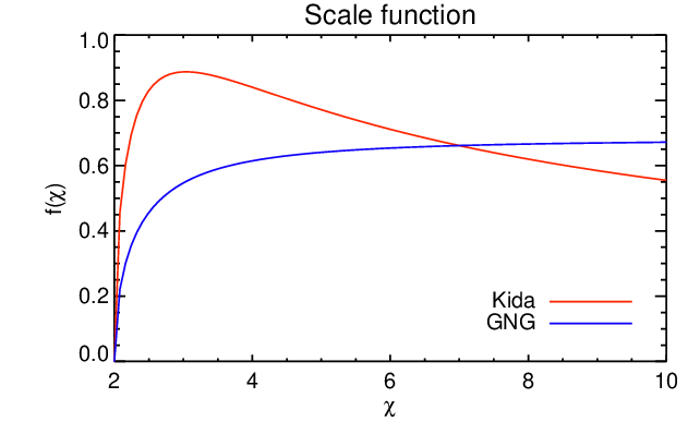
and depends on the vortex solution used. We plot for the Kida and GNG solutions in 1. They are defined in the real axis only for ( for ). The Goodman solution tends to an asymptote around 0.7. The Kida solution has a tail around in the interval of physical relevance ().
We show in 2, in the inertial frame, the dust distribution for =1 in a Kida vortex of embedded in a disk of aspect ratio =0.1, where is the stellocentric distance. We caution that this image extrapolates the spatial range of applicability of the shearing box approximation used to construct the solution.
It is worth noting that for certain vortex models and/or aspect-ratios, the Gaussian solution, Eq. (31), is in fact an exact solution to the dust-steady state equation, Eq. (27). We will explore this in more detail in Sect. V, but one can check this by inserting Eq. (31) into Eq. (27), and finding the condition for the coefficient of the trigonometric terms to vanish. In this special case, explicitly averaging over is not required to remove the -dependence from the problem.
IV.2. Gas distribution
Eq. (31) allows us to calculate the gas distribution. For that we recall that for tracer particles (), the dust distribution should mimic that of the gas. The distribution should thus be
| (36) |
with
| (37) |
and , the maximum gas density11 1 Note that Eq. (36) is the gas density averaged over at fixed . One may directly integrate the gas momenta equations to see that the gas density/pressure depends, in general, on both and ..
Notice that for the effect of diffusion cancels out. This is because the diffusion is proportional to the gradient of the dust-to-gas ratio (Eq. 2), which is zero for tracer particles.


V. Non-axisymmetric corrections
We now consider the non-axisymmetric problem (). We explicitly show that such effects are small in the vortex core provided the effective Stokes number is not large. These requirements will become apparent as we proceed through the solution method. In this section we consistently refer to “axisymmetric” as -symmetry in the coordinate system defined by Eqs. (18) and (19).
V.1. Conversion to ordinary differential equations
The dust density is periodic in the co-ordinate. We therefore seek solutions of the form
| (38) |
For convenience, we will drop the real part notation from now on. Inserting Eq. (38) into the partial differential equation (Eq. 27), multiplying by , and integrating the resulting expressions over the co-ordinate, we arrive at a set of coupled ordinary differential equations,
| (39) |
where , and
| (41) | |||||
where , , and
| (43) |
Note that is a function of the aspect-ratio depending on the vortex model. Eq. (39) holds for each except for for which the terms are absent. Each couples to through operators and . The axisymmetric problem is recovered by setting .
We expect to have even symmetry in because of the elliptical nature of the vortex streamlines. Henceforth we only consider even . We seek solutions with (where the prime denotes derivative with respect to the argument) and , so that at the origin, consistent with dust reaching maximal density there.
V.2. Operator properties
Consider
| (44) |
Then we find that
| (45) | |||||
| (46) | |||||
| (47) | |||||
The first two expressions will be useful in constructing nearly-axisymmetric solutions.
V.3. Exact axisymmetric solutions
It is useful to see how the formulation above connects with the axisymmetric solutions discussed in the previous section. Consider the special case where , so that Then the complete solution to Eq. (39) is with , and is an arbitrary constant. That is, if then the dust distribution is exactly axisymmetric.
V.3.1 Dust in a GNG vortex is axisymmetric
For the GNG vortex, one can verify that , implying dust density only depends on the ellipse under consideration, not the position along it. This is because the GNG vortex has no pressure gradient along the elliptical streamlines [16].
V.3.2 Condition for dust in a Kida vortex to be axisymmetric
For the Keplerian Kida vortex, we find
| (48) |
The dust distribution is exactly axisymmetric for aspect-ratio , which is also when the Keplerian Kida vortex has no pressure gradient along its elliptical streamlines [16].
V.4. Source term approximation
In preparation for constructing non-axisymmetric solutions, we here describe the source term approximation [117]. We assume that decreases with , so that in Eq. (39) the term has smallest magnitude. Neglecting it as a first approximation, we solve
| (49) |
The solutions are
| (50) |
with
| (51) |
for , and is arbitrary as before. Note that for odd because since we require . Then, by induction
| (52) |
for even .
The source term approximation assumes For given , the solution is consistent with this requirement if , corresponding to small effective Stokes number. However, this approximation will eventually fail for large because the solution above implies for . Thus the solution is only self-consistent for sufficiently small and/or . Nevertheless, we comment that the closed-formed solutions obtained here may be useful in an iterative scheme to obtain numerical solutions to the full set of ODE’s.
V.5. Weakly non-axisymmetric dust distributions
We are now ready to construct non-axisymmetric solutions. Consider a Keplerian Kida vortex with , meaning that the effective frictional force on the dust has a non-vanishing component along the fluid velocity vector. (I.e. dust particles are accelerated along the ellipse.) We assume non-axisymmetry in the dust distribution is sufficiently weak, so one may truncate the series solution at . Thus we set . Let
| (53) |
where represents the correction to the axisymmetric solution due to . The ODEs to be solved are
| (54) | ||||
| (55) |
To make further progress, at this stage we assume that the term in Eq. 55 can be neglected, so with given by the source term approximation. This means that
| (56) |
implying non-axisymmetry becomes significant for sufficiently large , and truncating the series at is no longer self-consistent. However, in practice the ratio is small. For example, inserting gives for and for . Since most of the dust is contained within , we conclude that non-axisymmetry is in general a small effect.
| (57) |
Collecting the above results and Taylor-expanding the ’s, our weakly non-axisymmetric solution for reads:
| (58) | ||||
| (59) |
where we have used the definition of and set without loss of generality. In the previous section, we obtained the axisymmetric solution assuming the non-axisymmetric components are negligible. Here, we see explicitly that the axisymmetric solution in fact leads to non-axisymmetry through the coupling terms, but these corrections are small for , because . We conclude that dust in the vortex core is effectively axisymmetric.
V.5.1 Consistency check
Using the above expression for , we can evaluate in order to assess our assumption that has a negligible contribution to . We find
| (60) | |||||
Provided that and is not large, this term is indeed small compared to the first term on the RHS of Eq. (55). For example, considering , for and we obtain . Even with , this ratio is not large. We conclude that our solution procedure above is self-consistent.
VI. Observational predictions
Having arrived at the “axisymmetric” solutions (in the - plane, Sect. IV), and shown that deviations from -symmetry are small (Sect. V), we go back to the solutions of Sect. IV to derive observational predictions.
VI.1. Dust - gas contrast
Eq. (31) and Eq. (36) also allows us to calculate the gas-dust density contrast, and, therefore, as a function of . For that, we calculate the volume integral of and . These, in turn, need the dependencies on the vertical coordinates . These are straightforward, being for the gas and for the dust, with [29]. Integrated over plus and minus infinity, these yield and , respectively. We have thus
| (61) | |||||
| (62) | |||||
Dividing Eq. (61) by Eq. (62), the ratio of the integrals in the left hand sides is the global dust-to-gas ratio, . The density enhancement factor is thus
| (64) |
where is an appropriate reference density. The full expression for the dust density is therefore
| (65) |
Eq. (64) shows that the dust-to-gas ratio at the origin (vortex center) is related to the total dust-to-gas mass ratio by a simple function of . In this enhancement, only a third (in log) is caused by sedimentation. The rest is due to in-plane vortex capturing. Midplane dust distributions for different values of are plotted in 3, as a function of .
VI.2. Trapped mass
VI.3. Dust density contrast
The contrast in the same orbit is found by calculating the minimum dust density and comparing it to Eq. (64). By substituting the gas solution (Eq. 36) into Eq. (31) we can write
| (67) |
which is the same result as found by [6], provided a suitable choice is made for (we do not assume a relationship between and because the turbulence in the vortex core is locally generated and unrelated to the disk turbulence, c.f., elliptic instability, Lesur & Papaloizou 62, Lyra & Klahr 66). The minimum densities occur at the boundary of the vortex, which is the sonic perimeter where shocks occur. Its limit is found by writing the vortex velocity (Eq. 8) as a Mach number
| (68) |
and setting . This yields the boundary at
| (69) |
where the subscript stands for sonic. The Kida solution asymptotically reaches , while the GNG solution asymptotically reaches . In the physical range of relevance (), they both yield values around , which matches the results of numerical simulations. Substituting Eq. (69) in Eq. (36), the gas density contrast is
| (70) |
For neither the Kida nor the GNG solutions does this quantity deviate much from unity. This is because the argument in the exponent tends asymptotically in both cases to small fractions of ; in the Kida case, in the GNG case.
VI.4. Measuring
Closed elliptic streamlines are subject to the elliptic instability, which leads to subsonic turbulence in the vortex core [62, 66]. To directly measure , the turbulent diffusion parameter, one would need to measure the turbulent velocity field. As , the Shakura-Sunyaev viscosity parameter [103], can be defined as the ratio of stress over pressure. If the turbulence is isotropic in the midplane, one can write
| (71) |
where is the rms of the turbulent velocities. The beam smearing would render the velocity field unresolved even for moderately close systems, so one should look for unresolved signatures. Spectroscopically, this extra rms velocity should have an effect similar to microturbulence, providing a slight extra broadening to the Doppler core of suitable spectral lines.
For gas temperatures ranging 20-200 K, assuming that the gas is a 5:2 hydrogen to helium mixture (mean molecular weight of 2.4), the isothermal sound speeds range 0.26-0.83 km/s. Considering that typical velocities of subsonic turbulence are 10% of the sound speed (), the typical velocity signal for 200 K would be of the order of 0.1 km/s. As [71] quote a sensitivity limit of 0.2 km/s for their ALMA observations of Oph IRS 48, only the 2 tail of the turbulent velocity field should be detectable.
If a direct determination of does not sound promising, an indirect way is possible by measuring and . The parameter can be determined via the dust-density contrast with Eqs. (67) and (70), or via the dust-gas contrast at maximum (Eq. 64). The Stokes number is
| (72) |
where is the particle radius and the particle internal density.
VI.5. Application to Oph IRS 48
We now apply our model to the observed Oph IRS 48 system, with the parameters derived by [71].The dust contrast in the same orbit is 130, which, according to Eq. (67) and Eq. (70) for , sets and for the Kida and GNG solutions, respectively. The values are close because the gas contrast is small (Eq. 70).
The dust temperature derived by the authors is 60 K. Assuming this is the same as the gas temperature, and a mean molecular weight of 2.4, the isothermal sound speed is . At =63 AU, around a star, this translates into an aspect ratio of , or AU. As for the particle radius, the ALMA data is sensitive up to mm, and we take this size to be representative.
The gas mass is quoted to range between 19-27 Jupiter masses, measured from a ring centered at 60 AU. The signal-to-noise is too low to derive a radial extent, but assuming it ranges 50-70 AU, the gas surface density should range 20-30 g cm2. We take =25 g cm2 as best estimate, which, for the scale height derived above, translates into .
For particles of material density , the Stokes number should then be . For , this translates into , meaning typical turbulent velocities in the vortex core at of the sound speed. These velocities fall squarely within the range expected for the elliptic instability [62, 66], that shows a maximum speed of 10% of the speed of sound.
As for the trapped mass, van der Marel et al. [71] measures 9 . For the typical interstellar dust-to-gas ratio of , Eq. (66) yields 6 and 17 for Kida and GNG, respectively. Given the approximations, assumptions, and uncertainties, the agreement within a factor 2 is remarkable.
Although these values seem reasonable, it should be noted that for Oph IRS 48 the candidate planet is at 20 AU, whereas the dust trap is at 63 AU. Even though the planet is supposed to be massive (planet-to-star mass ratio ), gaps are not expected to be that wide. The supposed vortex also seems to be very big, with a semiminor axis of 17 AU. For a temperature of 60 K, this corresponds to over 3, which is far from the expected from numerical simulations and Eq. (69). Relaxing the approximation that the gas and dust have the same temperature does little to solve the discrepancy. Because , a vortex six times bigger means a temperature thirty-six times hotter. This would bring the gas temperature above 2 000 K, which is unrealistic.
VII. Conclusions
We solve for the distribution of dust trapped in disk vortices, in steady state between gas drag, that tends to drive dust into the vortex, and diffusion, that expels it. Eqs. (31) and (34), with coefficient given by Eq. (64), are our result for a distribution with “axis-symmetry” in the coordinate system defined by Eqs. (18) and (19). That is, consisting of ellipses of equal aspect ratio as those of the gas vortex. The solution has some remarkable properties. It is a Gaussian of standard deviation , where, given the angular velocity of the vortex, is determined by three quantities. These are: the sonic length and gas scale height, ; the vortex aspect ratio ; and , the relative strength of drag to diffusion. The importance of this latter parameter had already been hinted upon by Cuzzi et al. [27] and Dubrulle et al. [29] in the context of steady states of dust sedimentation, and by Klahr & Henning [48] for vortices in the meridional plane. An insightful study by Jacquet et al. [52] emphasized the relevance of this parameter for global redistribution of solids. Birnstiel et al. [6] also find this to be the parameter of relevance in their semi-analytical model.
Transitional disks provide an interesting venue where to test the model in an astrophysical context, since all three parameters can be derivable from data. The vortex aspect ratio is readily observable, and follows from the temperature (). The parameter follows from the density contrast (either dust-gas contrast at maximum or dust constrast in the same orbit). Disentangling from in this parameter requires directly measuring at least one of these quantities. The diffusion parameter is in principle not equal to (the dimensionless gas viscosity of Shakura & Sunyaev 103), because the processes generating turbulence in the vortex and in the disk are different. The latter is supposedly the MRI, whereas the former is the elliptic or magneto-elliptic instability (see Lyra 64 and references therein). A direct measure of would require measuring the velocity field inside the vortex, that would appear spectroscopically as a slight extra line broadening. However, this would be difficult because the signal is too small. Measuring requires knowing the gas density and temperature, the particle radius and internal density. Of these, the internal density is difficult to measure directly and should be inferred by laboratory experiments. We apply the model to the Oph IRS 48 system, finding consistent values. The Stokes number for the 1.5 mm particles is estimated at , implying , and turbulent velocities in agreement with numerical simulations. The total dust masses we estimate are within a factor 2 of the measured value.
We also solve for the non-axisymmetric problem, showing that, for the vortex core, it is in general but a small correction. The solution is Eq. (38), with “radial” basis functions given by Eq. (50) and coefficients given by Eq. (52). In practice, the magnitude of the higher non-axisymmetric modes fall fast as increases, and only the term would provide an appreciable deviation from -symmetry. We find that non-axisymmetry in dust is associated with non-zero pressure gradients along elliptical streamlines of the vortex.
We recall that aside from planetary gap edges, self-sustained disk vortices may also result from either RWI at the boundary between the MRI-active and dead zones, or convective-like nonlinear baroclinic instabilities [47, 46, 91, 92, 62, 66, 97]. These processes, however, are not reasonable in the context of outer regions of transition disks: the outer edge of the dead zone is quite smooth [30, 53], whereas the RWI requires a sharp enough transition; as for the baroclinic instability, it requires finite thermal diffusion, whereas the thin outer disk is supposed to radiate efficiently. This leaves gap-edge RWI as the only currently known plausible mechanism to excite such vortices. However, this interpretation is not without difficulties, because, as noted in Sect. VI.5, the dust trap is too far out (63 AU) to be the result of a gas gap carved by a planet at 20 AU, and because its radial size (35 AU) would imply an unrealistic high gas temperature. Future modeling should aim at solving these discrepancies.
References
- [1] Adams, F, C. & Watkins, R. 1995, ApJ, 451, 314
- [2] Alexander, R. D., Clarke, C. J., & Pringle, J. E 2006, MNRAS, 369, 216
- [3] Andrews, S.M., Wilner, D.J., Espaillat, C., Hughes, A.M., Dullemond, C.P., McClure, M.K., Qi, C., & Brown, J.M. 2011, ApJ, 732, 42
- [4] Balbus, S. A. & Hawley, J. F. 1991, ApJ, 376, 214
- [5] Barge, P. & Sommeria, J. 1995, A&A, 295L, 1
- [6] Birnstiel, T., Dullemond, C. P., & Pinilla, P. 2013, A&A, 550L, 8
- [7] Birnstiel, T., Andrews, S. M., & Ercolano, B. 2012, A&A, 544, 79
- [8] Brauer, F., Dullemond, C.P., Johansen, A., Henning, Th., Klahr, H., & Natta, A. 2007, A&A, 469, 1169
- [9] Brown, J. M., Blake, G. A., Qi, C., Dullemond, C. P., Wilner, D. J., & Williams, J. P. 2009, ApJ, 704, 496
- [10] Bryden, G., Chen, X., Lin, D. N. C., Nelson, R. P., & Papaloizou, J. C. B. 1999, ApJ, 514, 344
- [11] Calvet, N., D’Alessio, P., Hartmann, L., Wilner, D., Walsh, A., & Sitko, M. 2002, ApJ, 568, 1008
- [12] Calvet, N., Muzerolle, J., Briceño, C., Hernández, J., Hartmann, L., Saucedo, J.L., & Gordon, K.D. 2004, AJ, 128, 1294
- [13] Calvet, N., D’Alessio, P., Watson, D. M., Franco-Hernández, R., Furlan, E., Green, J., Sutter, P. M., Forrest, W. J., Hartmann, L., Uchida, K. I., Keller, L. D.,Sargent, B., Najita, J., Herter, T. L., Barry, D. J., & Hall, P. 2005, ApJ, 630, 185
- [14] Casassus, S., Perez M., S., Jordán, A., Ménard, F., Cuadra, J., Schreiber, M. R., Hales, A. S., & Ercolano, B. 2012, ApJ, 754, 31
- [15] Casassus, S., van der Plas, G., Perez, S., Dent, W.R.F., Fomalont, E., Hagelberg, J., Hales, A., Jordán, A., Mawet, D., Ménard, F., Wootten, A., Wilner, D., Hughes, M., Schreiber, M.R., Girard, J.H., Ercolano, B., Canovas, H., Román, P., & Salinas, V. 2013, Nature, 493, 191
- [16] Chang, P. & Oishi, J.S. 2010, ApJ, 721, 1593
- [17] Chavanis, P.-H. 2000, A&A, 356, 1089
- [18] Charnoz, S., Fouchet, L., Aleon, J., & Moreira, M. 2011, ApJ, 737, 33
- [19] Cieza, L.A., Swift, J.J., Mathews, G.S., & Williams, J.P. 2008, ApJ, 686, 115
- [20] Cieza, L.A., Schreiber, M.R., Romero, G.A., Mora, M.D., Merín, B., Swift, J.J., Orellana, M., Williams, J.P., Harvey, P.M., & Evans, N.J. 2010, ApJ, 712, 925
- [21] Clarke, C.J. & Owen, J.E. 2013, MNRAS, accepted, arXiv:1305.2483
- [22] Clarke, C. J.; Pringle, J. E. 1988, MNRAS, 235, 365
- [23] Corder, S., Eisner, J., & Sargent, A. 2005, ApJ, 622, 133
- [24] Currie, Th., Lada, C.J., Plavchan, P., Robitaille, T.P., Irwin, J., & Kenyon, S.J. 2009, ApJ, 698, 1
- [25] Currie, Th. 2010, arXiv1002.1715C
- [26] Currie, Th. & Sicilia-Aguilar, A. 2011, ApJ, 732, 24
- [27] Cuzzi, J.N., Dobrovolskis, A.R., & Champney, J.M. 1993, Icarus, 106, 102
- [28] Dominik, C. & Dullemond, C. P. 2008, A&A, 491, 663
- [29] Dubrulle, B., Morfill, G., & Sterzik, M. 1995, Icarus, 114, 237
- [30] Dzyurkevich, N., Turner, N.J., Henning, Th., & Kley, W. 2013, ApJ, 765, 114
- [31] Espaillat, C., Calvet, N., Luhman, K.L., Muzerolle, J., & D’Alessio, P. 2008, ApJ, 682L, 125
- [32] Gauvin, L.S. & Strom, K.M. 1992, ApJ, 385, 217
- [33] Godon, P. & Livio, M. 1999, ApJ, 523, 350
- [34] Godon, P. & Livio, M. 2000, ApJ, 537, 396
- [35] Goldreich, P. & Ward, W.R. 1973, ApJ, 183, 1051
- [36] Goodman, J., Narayan, R., & Goldreich, P. 1987, MNRAS, 225, 695
- [37] Hawley, J.F. 1987, MNRAS, 225, 677
- [38] Lovelace, R.V.E. & Hohlfeld, R.G. 1978, ApJ, 221, 51
- [39] Inaba, S. & Barge, P. 2006, ApJ, 649, 415
- [40] Ireland, M. J. & Kraus, A. L. 2008, ApJ, 678L, 59
- [41] Isella, A., Pérez, L.M., Carpenter, J.M., Ricci, L., Andrews, S., & Rosenfeld, K. 2013, ApJ, submitted
- [42] Isella, A., Pérez, L.M., & Carpenter, J.M. 2012, ApJ, 747, 136
- [43] Johansen, A., Andersen, A. C., & Brandenburg, A. 2004, 417, 361
- [44] Johansen, A., Oishi, J. S., Mac Low, M.-M., Klahr, H., Henning, Th., & Youdin, A. 2007, Nature, 448, 1022
- [45] Kida, S. 1981, J. Phys. Soc. Jpn., 50, 351
- [46] Klahr, H. 2004, ApJ, 606, 1070
- [47] Klahr, H. & Bodenheimer, P. 2003, ApJ, 582, 869
- [48] Klahr, H.H. & Henning, Th. 1997, Icarus, 128, 213
- [49] Klahr, H. & Kley, W. 2006, A&A, 445, 747
- [50] Kley, W., Müller, T. W. A., Kolb, S. M., Benítez-Llambay, P., & Masset, F. 2012, A&A, 546, 99
- [51] Kley, W. & Nelson, R. P. 2012, ARA&A, 50, 211
- [52] Jacquet, E., Gounelle, M., & Fromang, S. 2012, Icarus, 220, 162
- [53] Landry, R., Dodson-Robinson, S.E., Turner, N.J., & Abram, G. 2013, arXiv1305.0770
- [54] Lin, D.N.C. & Papaloizou, J. 1986a, ApJ, 307, 395
- [55] Lin, D.N.C. & Papaloizou, J. 1986b, ApJ, 309, 846
- [56] Lin, M.-K. & Papaloizou, J.C.B. 2011, MNRAS, 415, 1426
- [57] Lin, M.-K. & Papaloizou, J.C.B. 2011, MNRAS, 415, 1445
- [58] Lin, M.-K. & Papaloizou, J.C.B. 2012, MNRAS, 421, 780
- [59] Lin, M.-K. 2012, ApJ, 754, 21
- [60] Lin, M.-K. 2012, MNRAS, 426, 3211
- [61] Lin, M.-K. 2013, ApJ, 765, 84
- [62] Lesur, G. & Papaloizou, J.C.B. 2010, A&A, 513, 60
- [63] Lovelace, R.V.E., Li, H., Colgate, S.A., & Nelson, A. F. 1999, ApJ, 513, 805
- [64] Lyra, W. 2013, in Instabilities and Structures in Proto-Planetary Disks, Marseille, France, Edited by P. Barge; L. Jorda; EPJ Web of Conferences, Volume 46, id.04003
- [65] Lyra, W. & Mac Low, M.-M. 2012, ApJ, 756, 62
- [66] Lyra, W. & Klahr, H. 2011, A&A, 527A, 138
- [67] Lyra, W., Johansen, A., Zsom, A., Klahr, H., Piskunov, N. 2009b, A&A, 497, 869
- [68] Lyra, W., Johansen, A., Klahr, H., Piskunov, N. 2009a, A&A, 493, 1125
- [69] Lyra, W., Johansen, A., Klahr, H., & Piskunov, N. 2008, A&A, 491, L41
- [70] Lyttleton, R.A. 1972, MNRAS, 160, 255
- [71] van der Marel, N., van Dishoeck, E. F., Bruderer, S., Birnstiel, T., Pinilla, P., Dullemond, C. P., van Kempen, T. A., Schmalzl, M., Brown, J. M., Herczeg, G. J., Matthews, G. S., & Geers, V. 2013, Science, 340, 1199
- [72] Masset, F. & Snellgrove, M. 2001, MNRAS, 320L, 55
- [73] Méheut, H., Casse, F., Varnière, P., & Tagger M. 2010, A&A, 516, 31
- [74] Méheut H., Cong, Y., & Lai, D. 2012, MNRAS, 422, 2399
- [75] Méheut H., Keppens, R., Casse, F., & Benz, W. 2012, A&A, 542A, 9
- [76] Méheut, H., Meliani, Z., Varnière, P., & Benz, W. 2012, A&A, 545, 134
- [77] Merín, B., Brown, J. M., Oliveira, I., Herczeg, G.J., van Dishoeck, E.F., Bottinelli, S., Evans, N.J., Cieza, L., Spezzi, L., Alcalá, J.M., Harvey, P.M., Blake, G.A., Bayo, A., Geers, V.G., Lahuis, F., Prusti, T., Augereau, J.-C., Olofsson, J., Walter, F.M., & Chiu, K. 2010, ApJ, 718, 1200
- [78] Morfill, G. E. & Voelk, H. J. 1984, ApJ, 287, 371
- [79] Muto, T., Grady, C. A., Hashimoto, J., Fukagawa, M., Hornbeck, J. B. et al. 2012, ApJ, 748L, 22
- [80] Muzerolle, J., Adame, L., D’Alessio, P., Calvet, N., Luhman, K.L., Muench, A.A., Lada, C.J., Rieke, G.H., Siegler, N., Trilling, D.E., Young, E.T., Allen, L., Hartmann, L., & Megeath, Th. 2006, ApJ, 643, 1003
- [81] Muzerolle, J., Allen, L.E., Megeath, Th., Hernández, J., & Gutermuth, R.A. 2010, ApJ, 708, 1107
- [82] Najita, J.R., Strom, S.E., & Muzerolle, J. 2007, MNRAS, 378, 369
- [83] Nelson, R.P., Papaloizou, J.C.B., Masset, F., & Kley, W. 2000, MNRAS, 318, 18
- [84] Oppenheimer, B.R., Brenner, D., Hinkley, S., Zimmerman, N., Sivaramakrishnan, A., Soummer, R., Kuhn, J., Graham, J.R., Perrin, M., Lloyd, J.P., Roberts, L.C., & Harrington, D.M. 2008, ApJ, 679, 1574
- [85] Owen, J.E., Ercolano, B., Clarke, C.J., & Alexander, R.D. 2010, MNRAS, 401, 1415
- [86] Paardekooper, S.-J. & Mellema, G. 2004, A&A, 425L, 9
- [87] Papaloizou, J. & Lin, D.N.C. 1984, ApJ, 285, 818
- [88] Papaloizou, J.C.B. & Pringle, J.E. 1984, MNRAS, 208, 721
- [89] Papaloizou, J.C.B. & Pringle, J.E. 1985, MNRAS, 213, 799
- [90] Pascucci, I. & Sterzik, M. 2009, ApJ, 702, 724
- [91] Petersen, M. R., Julien, K., Stewart, G. R. 2007a, ApJ, 658, 1236
- [92] Petersen, M. R., Stewart, G. R., Julien, K. 2007b, ApJ, 658, 1252
- [93] Piétu, V., Guilloteau, S., & Dutrey, A. 2005, A&A, 443, 945
- [94] Pinilla, P., Benisty, M., & Birnstiel, T. 2012b, A&A, 545, 81
- [95] Pinilla, P., Birnstiel, T., Ricci, L., Dullemond, C.P., Uribe, A.L., Testi, L., & Natta, A. 2012a, A&A, 538, 114
- [96] Quillen, A.C., Blackman, E.G., Frank, A., & Varnière, P. 2004, ApJ, 612, 137
- [97] Raettig, N., Lyra, W., & Klahr, H. 2013, ApJ, 765, 115
- [98] Regály, Zs., Juhász, A., Sándor, Zs, & Dullemond, C.P. 2012, MNRAS, 419, 1701
- [99] Regev, O. & Umurhan, O. M. 2008, A&A, 468, 341
- [100] Rosotti, G.P., Ercolano, B., Owen, J.E., & Armitage, P.J. 2013, MNRAS, 430, 1392
- [101] Safronov, V. S. 1969, Evoliutsiia Doplanetnogo Oblaka (English transl: Evolution of the Protoplanetary Cloud and Formation of Earth and the Planets, NASA Tech. Trans. F-677, Jerusalem: Israel Sci. Transl., 1972)
- [102] Sicilia-Aguilar, A., Hartmann, L.W., Fürész, G., Henning, Th., Dullemond, C., & Brandner, W. 2006, AJ, 132, 2135
- [103] Shakura, N. I. & Sunyaev, R. A. 1973, A&A, 24, 337
- [104] Skrutskie, M. F., Dutkevitch, D., Strom, S.E., Edwards, S., Strom, K.M., & Shure, M.A. 1990, AJ, 99, 1187
- [105] Strom, K.M., Strom, S.E., Edwards, S., Cabrit, S., & Skrutskie, M.F. 1989, AJ, 97, 1451
- [106] Tagger M. 2001, A&A, 380, 750
- [107] Tang, Y.-W., Guilloteau, S., Piétu, V., Dutrey, A., Ohashi, N., & Ho, P.T.P. 2012, A&A, 547, 84
- [108] Tanga P., Babiano, A., Dubrulle, B., & Provenzale, A. 1996, Icarus, 121, 158
- [109] Toomre, A. 1981, What amplifies the spirals. In The Structure and Evolution of Normal Galaxies, Proceedings of the Advanced Study Institute, Cambridge, England, Cambridge and New York, Cambridge University Press, 1981, p.111-136.
- [110] de Val-Borro, M., Artymowicz, P., D’Angelo, G., Peplinski, A. 2007, A&A, 471, 1043
- [111] de Val-Borro, M., Edgar, R.G., Artymowicz, P., Ciecielag, P., Cresswell, P., D’Angelo, G., Delgado-Donate, E.J., Dirksen, G., Fromang, S., Gawryszczak, A., Klahr, H., Kley, W., Lyra, W., Masset, F., Mellema, G., Nelson, R., Paardekooper, S.-J., Peplinski, A., Pierens, A., Plewa, T., Rice, K., Schäfer, C., & Speith, R. 2006, MNRAS
- [112] Varnière, P. & Tagger, M. 2006, A&A, 446, 13
- [113] Wolk, S.J. & Walter, F.M. 1996, AJ, 111, 2066
- [114] Youdin, A. N. & Goodman, J. 2005, ApJ, 620, 459
- [115] Youdin, A. N. & Shu, F. H. 2002, ApJ, 580, 494
- [116] Youdin, A. 2008arXiv:0807.1114
- [117] Zhang, H., & Lai, D. 2006, MNRAS, 368, 917
- [118] Zhu, Zh., Nelson, R.P., Hartmann, L., Espaillat, C., & Calvet, N. 2011, ApJ, 729, 47
- [119] Zsom, A., Ormel, C.W., Dullemond, C.P., & Henning, Th. 2011, A&A, 534, 73