On Analyzing Estimation Errors due to Constrained Connections in Online Review Systems
Abstract
In this work, we study how constrained connections can cause estimation errors in online review systems. Constrained connection is the phenomenon that a reviewer can only review a subset of products/services due to reviewer’s narrow range of interests or limited attention capacity. We find that reviewers’ constrained connections will cause poor inference performance, both from the measurements of estimation accuracy and Bayesian Cramér Rao lower bound.
I Introduction
Online reviews are more and more important factors for customers to decide whether to buy a product or service in online markets. Due to this reason, online review systems have become battle fields for companies to compete with each other by hiring “Internet Water Mercenaries”, which are also known as paid spammers, to post favorable reviews about their products/services and negative reviews about their competitors’. These fake reviews disturb customers’ judgments on the quality of products/services and ruin companies’ reputation. Hence, an always important problem in online review systems is how to accurately obtain the truth of both reviewers (e.g., the reviewer is a spammer or non-spammer) and items (e.g., the product/service is good or bad) according to unreliable online reviews.
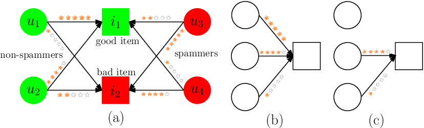
In previous studies[10, 1], most of the works ignore the function of the underlying topology of ORS. The topology of an online review system is a bipartite graph representing which reviewers can review which items. Many works explicitly or implicitly assume that reviewers can review all the other items, such as the example shown in Fig. 1(a). In fact, a reviewer can only review a subset of items in real-world, which results in constrained connections for each reviewer in the topology. The constrained connections may be because of either the reviewer’s narrow range of interests or the reviewer’s limited attention capacity (that he cannot afford to review all other items). The constrained connections can affect the performance of jointly estimating the truth of reviewers and items. For example, let us consider a simplest online review system that consists of three reviewers and one item. If we assume the majority of reviewers are non-spammers (that is true in real-world), then in the case of Fig. 1(b), from this topology and reviews by each reviewer we can infer with high confidence that the item is probably good and the bottom reviewer is likely to be a spammer. However, in the case of (c), we cannot obtain a high confidence conclusion because we do not know the reviews of the top reviewer.
The simple example tells us that different topologies of ORS along with unreliable reviews contain different amounts of information for jointly estimating the truth of reviewers and items. Actually, connections between reviewers and items act as constraints in such systems. They constrain the joint probability distribution of the truth of reviewer-item pairs they connect. For example, a non-spammer usually gives good (bad) items good (bad) reviews with high probability, which indicates that the truth of a reviewer and the truth of an item he reviewed are related. Hence the topology of the ORS yields a set of constraints that the truth of reviewers and items must obey, and these constraints help to reduce the uncertainty of parameters in the system.
In order to compare the amounts of information contained in different topologies (and reviews), we calculate the Bayesian Cramér Rao lower bound (BCRLB) of maximum a posteriori estimator (MAPE) in such systems for different bipartite graph models. We find that BCRLB varies for different topologies. This indicates that for some topologies the truth become much difficult to be estimated by any MAPEs.
II Background and Basic Results
II-A Data Model
Following the existing works[7, 5, 6], we assume that there are a set of reviewers and a set of items in an online review system. Each item is associated with a binary label , which is considered to be a random variable representing the quality of item , e.g., if item is good; if is bad. Each reviewer can choose items to review. A review represents the reviewer’s attitude to an item. If we use to denote ’s review to , then (or ) means that reviewer considers item to be good (or bad). However, reviewers are not always accurate to review items, and we use to represent the probability that the reviewer can give correct reviews, i.e., . In practice, it is reasonable to assume that the majority of reviewers have . This is achieved by putting a prior distribution on . A nature choice of such a prior is the beta distribution, i.e., , where .
Be different from previous works, in this work we assume that a reviewer can not freely choose which items to review. The reasons may be the reviewer’s narrow range of interests, limited attention capacity, and so on. If reviewer can review item , we connect and by an edge . This forms a bipartite graph , where is the set of edges. Furthermore, we use to denote the set of items that can review, and we use to denote the set of reviewers who can review .
To make the aforementioned model more general, we assume that items to be reviewed by reviewers are chosen independently with replacement constrained by graph 11 1 Consider items to be shops, each time a consumer buy a product from a shop, he can review the shop.. This forms a collection of review samples where denotes the -th sample representing some reviewer gives some item a review . Since items are chosen with replacement, we may observe that reviewer reviews item many times. We use to represent the number of times gives a review in the samples . Note that satisfies .
Our goal is to study how can affect the estimation accuracy when using to estimate and .
II-B Maximum A Posteriori Estimator
A convenient way to estimate parameters of the previous model is by considering as parameters and as hidden variables[3]. David and Skene[3] presented an expectation maximization (EM) approach to maximize the likelihood. Here we propose to maximize the posteriori of which can include the priori information of . That is,
| (1) |
E-Step: In the E-Step, we need to calculate the probability of hidden variables given the other variables , which can be factorized to . Here denotes the reviews in the samples that are related to item . If we denote each factor by , then we can obtain
| (2) | ||||
| (3) | ||||
| (4) | ||||
| (5) | ||||
| (6) |
M-Step: In the M-Step, we need to solve
| (7) | ||||
| (8) | ||||
| (9) |
which gives us the following result
| (10) |
Here, is the set of reviews given by reviewer .
The E-step and M-step of the EM algorithm implicitly defines an estimator of , i.e., . Since is related to , then is also related to . To understand how can affect the MAP estimator, we go to study the Mean Squared Errors of .
III Estimation Errors Analysis
III-A Lower Bound on Estimation Errors
The Mean Squared Error of is defined as , which is lower bounded by the Bayesian Cramér Rao lower bound (BCRLB) under some conditions[9, Chapter 2]. We rewrite Eq. (217) in Van Trees’ book [9, Page 73] and obtain the following relationship
| (11) |
where
| (12) |
is the element of Fisher information matrix .
The above relationship requires that is weakly unbiased[9, Chapter 2], which is unknown for the MAP estimator defined by EM algorithm. However, it is known that under general conditions, for large , the posterior distribution of can be approximated by normal distribution[2, 9, 4, 8]
where is the observed Fisher information matrix, and each element of is defined by
The above conclusion tells us that defined by the EM algorithm is a consistent estimator of with covariance matrix determined by . For different ’s, the estimator will have different covariance matrices. We can compare the estimation errors by evaluating ’s on different bipartite graphs. In the following, we find that is a diagonal matrix and it can be efficiently computed in combining with the EM procedure.
III-B Obtaining BCRLB in Combining with EM Procedure
Because , or equivalently
| (13) |
Then
| (14) | ||||
| (15) | ||||
| (16) | ||||
| (17) |
The first item of RHS is
| (18) | ||||
| (19) |
and if . The second item of RHS is
| (20) |
and if . Finally, we obtain the observed Fisher information matrix
| (21) |
and if .
This indicates that is a diagonal matrix. Note that Eq. (21) is convex, gets the minimum value at and gets the maximum value at or . This tells us that is most uncertain when and most certain at or . This is consistent with intuition as can be considered as the parameter of a Bernouli distribution.
IV Empirical Results
To study how constrained connections can affect the estimation accuracy of MAPE, we first present several bipartite graph models and then study how these models affect the performance of MAPE measured by the accuracy of classifying items and BCRLBs.
IV-A Bipartite Graph Models
IV-A1 Random Graph Model
Each edge in is formed by uniformly choosing a reviewer and uniformly choosing an item .
IV-A2 Item Preferential Attachment Graph Model
The assumption of this model is that popular items are more easily to receive reviews. Hence, an edge in is formed by uniformly random choosing a reviewer , and choosing item with probability proportion to ’s degree in .
IV-A3 Reviewer and Item Preferential Attachment Graph Model
We can also assume that a reviewer who is more active is more likely to review items. Hence, an edge in is formed by choosing a reviewer with probability proportion to ’s degree, and choosing item with probability proportion to ’s degree in .
IV-B Building Ground Truth Known Datasets
Given a graph built by one of the above models, we describe the procedure of generating review samples .
We specify a set of reviewers and items. Suppose that each user ’s parameter is chosen from beta prior distribution , i.e., reviewer gives correct review with prior probability . For each item , we randomly assign a label by flipping a fair coin, i.e., . The procedure of generating is as follows.
IV-C Comparing Items Inference Accuracy Under Different Graphs
In the first experiment, we compare classification accuracy of items under different graph models. We set an item with label (or ) if (or ). The accuracy is defined as
where and are the true positive and true negative respectively. and are positive and negative respectively. Accuracy describes the fraction of items that can be corrected inferred.
The results are shown in Fig. 2. We first generated graphs with number of nodes and varying number of edges () using different graph models. In each figure, we generated review samples of different sizes (), and show accuracy of inferring items averaged over 100 experiments respectively. We observe that when increases, the accuracy also increases and approaches 1. This confirms that the MAPE estimator is asymptotically unbiased. For different graph models, we observe that the accuracy on is larger than the other two models. This indicates that constrained connections will make the inference performance poor. However, the accuracy curves on and are approximately the same. This indicates that more constrained may not always decrease accuracy. To distinguish the difference of different constrained connections clearly, we study their difference of BCRLBs.


IV-D Comparing Estimation Errors Under Different Graphs
In the second experiment, we study how different graph modes affect the BCRLBs. The settings are same as in the previous experiment. We compare the average rooted mean squared error (RMSE) (defined as ) lower bound over different graph models in Fig. 3.
The RMSE decreases approximately with rate over all the graphs. For different graphs, when is large (we do not consider BCRLB for small n, because MAPE is biased when is small), RMSE on has the largest lower bound, then comes and RMSE on has the lowest lower bound. This indicates, when more constraints are added on graphs, the RMSE of any MAPEs will always become worse.


V Conclusion
The constrained connections are common in real world. A reviewer cannot review all the items due to various reasons in online review systems. In this study, we find that this constrained connection will always cause poor inference performance, both from the viewpoints of inference accuracy and RMSE lower bound.
References
- [1] Leman Akoglu, Rishi Chandy, and Christos Faloutsos. Opinion fraud detection in online reviews by network effects. ICWSM, 2013.
- [2] Harald Cramér. Mathematical Methods of Statistics. Princeton University Press, Princeton, New Jersey, 1946.
- [3] A. P. Dawid and A. M. Skene. Maximum likelihood estimation of observeerror-rates using the em algorithm. JSTOR, 1979.
- [4] Bradley Efron and David V. Hinkley. Assessing the accuracy of the maximum lielihood estimator: Observed versus expected fisher information. JSTOR, 65:457–482, 1978.
- [5] David R. Karger, Sewoong Oh, and Devavrat Shah. Iterative learning for reliable crowdsourcing systems. NIPS, 2011.
- [6] Qiang Liu, Jian Peng, and Alexander Ihler. Variational inference for crowdsourcing. NIPS, 2012.
- [7] Vikas C. Raykar, Shipeng Yu, Linda H. Zhao, Gerardo Hermosillo Valadez, Charles Florin, and Luca Bogoni. Learning from crowds. Journal of Machine Learning Research, 2010.
- [8] Martin A. Tanner. Toos for Statistics Inference: Methods for the Exploration of Posterior Distribution and Likelihood Functions. Springer Series in Statistics, 3rd edition, 2006.
- [9] H.L. Van Trees. Detection, Estimation, and Modulation Theory. Wiley, 1st edition, 1968.
- [10] Guan Wang, Sihong Xie, Bing Liu, and Philip S. Yu. Review graph based online store review spammer detection. ICDM, 2011.